Dual fermionic variables and renormalization group approach to junctions of strongly interacting quantum wires

Abstract

Making a combined use of bosonization and fermionization techniques, we build nonlocal transformations between dual fermion operators, describing junctions of strongly interacting spinful one-dimensional quantum wires. Our approach allows for trading strongly interacting (in the original coordinates) fermionic Hamiltonians for weakly interacting (in the dual coordinates) ones. It enables us to generalize to the strongly interacting regime the fermionic renormalization group approach to weakly interacting junctions. As a result, on one hand, we are able to pertinently complement the information about the phase diagram of the junction obtained within bosonization approach; on the other hand, we map out the full crossover of the conductance tensors between any two fixed points in the phase diagram connected by a renormalization group trajectory.

I Introduction

Many-electron systems, such as conduction electrons in a metal, are typically well-described by Landau’s Fermi liquid theory (LFLT), which is capable of successfully accounting for the main effects of electronic interaction Landau (1957a, b, 1958); Abrikosov et al. (1963). LFLT’s basic assumption is that, close to the Fermi surface, low-energy elementary ”quasiparticle” excitations of the interacting electron liquid are in one-to-one correspondence with particle- and hole-excitations in the noninteracting Fermi gas. This corresponds to a nonzero overlap between the quasiparticle wave function in the Fermi liquid and the electron/hole wave function in the noninteracting Fermi gas, which is reflected by a coefficient $Z_{F}$ of the quasiparticle peak at the Fermi surface in the spectral density of states that is finite though, in general, $<1$ ($Z_{F}=1$ corresponds to the noninteracting limit). The ”adiabatic deformability” of quasiparticles to electrons and/or holes by smoothly switching off the interaction allows, for instance, to address transport in a Fermi liquid in a similar way to what is done using scattering approach in a noninteracting Fermi gas, etc. Fisher and Glazman (1997).

LFLT is grounded on the possibility of obtaining reliable results by perturbatively treating the electronic interaction Abrikosov et al. (1963); Nozières (1964). This is strictly related to the small rate of multi-particle inelastic processes, in which, due to the interaction, an electron/hole emits electron-hole pairs. While this is typically the case in systems with spatial dimension $d$ higher than one, in one-dimensional systems, the proliferation of particle-hole pair emission at low energies leads to a diverging corresponding rate, which makes the quasiparticle peak disappear ($Z_{F}=0$). As a result, the interaction cannot be dealt with perturbatively and one has rather to resort to nonperturbative techniques, allowing for summing over infinite sets of diagrams Sólyom (1979); Shankar (1994); Polchinski (1993). The breakdown of LFLT in one-dimensional interacting electronic systems (interacting ”quantum wires” - QW’s) reveals itself in a series of physical contexts, the more remarkable of which is the transport across an interacting QW in the presence of a constriction, or a weak link, or the conductance of a junction of QWs, with or without spin Furusaki and Nagaosa (1993); Kane and Fisher (1992a, b); Matveev et al. (1993); Yue et al. (1994); Nazarov and Glazman (2003); Nayak et al. (1999); Chen et al. (2002); Lal et al. (2002); Pham et al. (2003); Chamon et al. (2003); Oshikawa et al. (2006); Rao and Sen (2004); Hou and Chamon (2008). Moreover, due to the remarkable correspondence between fermionic- and spin-bosonic one-dimensional lattice models encoded in the Jordan-Wigner fermionic representation of quantum spin-1/2 spin operators Jordan and Wigner (1928), a number of bosonic realizations of one-dimensional models of interacting fermions have been proposed in bosonic systems, such as quantum spin chains Eggert and Affleck (1992); Affleck (1998); Crampe and Trombettoni (2013); Tsvelik (2013); Reyes and Tsvelik (2005); Giuliano et al. (2013), quantum Josephson junction networks Glazman and Larkin (1997); Giuliano and Sodano (2010); Cirillo et al. (2011), or topological Kondo-type systems Béri and Cooper (2012); Galpin et al. (2014); Béri (2013); Eriksson et al. (2014a, b).

Formally, interacting electrons in one dimension are commonly treated within Tomonaga-Luttinger liquid (TLL)-approach Tomonaga (1955); Luttinger (1963). TLL formalism provides a general description of low-energy physics of a one-dimensional interacting electronic system in terms of collective bosonic excitations (charge- and/or spin-plasmons). Electronic operators are realized as nonlinear vertex operators of the bosonic fields Haldane (1981a, b). As for what concerns transport properties, the most striking prediction of the TLL-approach is possibly the power-law dependence of the conductance on the low-energy reference scale (”infrared cutoff”), which is typically identified with the (Boltzmann constant times the) temperature, or with the (Fermi velocity times the) inverse system length (”finite-size gap”) in a dc transport measurement, or with $eV$, with $V$ being an applied voltage, in a nonequilibrium experiment. While TLL-formalism poses no particular constraints on the strength of the ”bulk” interaction within the quantum wires, it suffers of limitations, when used to describe transport across impurities in an interacting quantum wire, or conduction properties at a junction of quantum wires (generically referred to, in the following of this section, as quantum impurities in the quantum wire). Parametrizing the spatial coordinate in each wire with $x(\geq 0)$, within the TLL-framework, a junction of quantum wires is mapped onto a model of $K$-one dimensional TLLs (one per each wire), interacting with each other by means of a ”boundary interaction” localized at $x=0$. Dealing with such a class of boundary problems requires pertinently setting the boundary conditions on the plasmon fields at $x=0$. While in some very special cases the boundary conditions can be written as simple linear relations between the plasmon fields, in general they cannot. This is a consequence of the nonlinearity of the relations between bosonic and fermionic fields: even linear conditions among the fermionic fields are traded for highly nonlinear conditions in the bosonic fields. As a consequence, except at the fixed points of the boundary phase diagram, where the boundary conditions are ”conformal”, that is, linear in the bosonic fields, the boundary interaction can only be dealt with perturbatively, with respect to the closest conformal fixed point Das et al. (2006); Aristov (2011). With very few remarkable exceptions, where the junction model Hamiltonian maps onto some exactly solvable model Fendley et al. (1995a, b, c), the only way for recovering ”global” (i.e., not necessarily in the vicinity of a conformal fixed point) informations about the phase diagram and the corresponding scaling of the conductance, is by just making educated guesses from the global topology of the fixed-point manifold of the phase diagram. Recently, the bosonization approach in combination with zero-temperature numerics has successfully been employed to compute the junction conductance by relating it to the asymptotic behavior of certain static correlation functions. Correspondingly, the length scale over which the asymptotic behavior emerges has been worked out, as well Rahmani et al. (2010, 2012). Also, numerical calculations of the finite-temperature junction conductance can be performed by using quantum Monte Carlo approach Sedlmayr et al. (2014) or, likely, by implementing some pertinently adapted version of the finite-temperature density matrix renormalization group approach to quantum spin chains Feiguin and White (2005); Karrasch et al. (2012).

Alternatively, one may not be required to give up using fermionic coordinates, by employing a systematic renormalization group (RG) procedure to treat the effects of the bulk interaction on the scattering amplitudes at the junction. Among the various possible ways of implementing RG for junctions of interacting QWs, the two most effective (and widely used) ones are certainly the poor man’s fermionic renormalization group (FRG)-approach, based upon a systematic summation of the “leading-log” divergences of the $S$-matrix elements at the Fermi momentum and typically yielding equations that can be analytically treated Matveev et al. (1993); Yue et al. (1994); Lal et al. (2002); Nazarov and Glazman (2003), and the functional renormalization group (fRG)-approach, based on the functional renormalization group method, leading to a set of coupled differential equations for the vertex part that, typically, can only be numerically treated Meden et al. (2003); Andergassen et al. (2004); Meden et al. (2005); Enss et al. (2005); Andergassen et al. (2006); Barnabe-Theriault et al. (2005a); Meden et al. (2006); Barnabe-Theriault et al. (2005b); Janzen et al. (2006); Jakobs et al. (2007). Both approaches are expected to apply only for a sufficiently weak electronic interaction in the quantum wires and, in this sense, they are less general than the TLL-approach, which applies even for a strong bulk interaction. Nevertheless, at variance with the TLL-approach, a RG-approach based on the use of fermionic coordinates leads to equations for the $S$-matrix elements valid at any scale and, thus, it allows for recovering the full scaling of the conductance, all the way down to the infrared cutoff.

Aside from the remarkable merit of providing analytically tractable RG-flow equations, the FRG-approach, when applied to interacting spinful electrons, also accounts for the backscattering bulk interaction, which is usually neglected in the TLL-framework Matveev et al. (1993); Yue et al. (1994). Moreover, it can be readily generalized to describe junctions involving superconducting contacts, at the price of doubling the set of degrees of freedom, to treat particle- and hole-excitations on the same footing Titov et al. (2006). Nevertheless, FRG is known to suffer of limitations, when used to describe the crossover towards ”healed” fixed points, where quantum impurities are renormalized towards boundary conditions corresponding to perfect conduction properties. In particular, this leads to a scaling equation for the conductance which, in the pertinent asymptotic regime, is not consistent with the one obtained from the bosonization approach. Using the fRG-approach allows for taking care of this flaw, as the fRG-technique typically takes into account the mutual feedback from all the single-fermion scattering channels, and not only those from scattering processes between different Fermi points (see Ref. [Meden et al., 2006] for a detailed discussion of this point and for a careful comparison between FRG- and fRG-approaches). In fact, fRG appears to be generically more accurate than FRG (which can be in fact recovered from fRG under suitable approximations Meden et al. (2006)). Both approaches suffer, however, of the limitation on the bulk interaction, which must be weak, in order for the technique to be reliably applicable.

To overcome such a limitation, in this paper, we study a junction of spinful interacting QWs by making a combined use of bosonization and fermionization, that is, we go back and forth from fermionic to bosonic coordinates, and vice versa, to build ”dual-fermion” representations of the junction in strongly interacting regimes. In resorting from a bosonic to a fermionic problem, our approach is reminiscent of the refermionization scheme used in Ref. [Schulz, 1980] to discuss the large-distance behavior of the classical sine-Gordon model at the commensurate-incommensurate phase transition. Specifically, in Schulz (1980) the refermionization allows for singling out at criticality the low-energy two-fermion excitations from the one-fermion ones and to prove that the latter ones keep gapped along the phase transitions and do not contribute to the large-distance scaling of the correlations. At variance, in our case it is the second of a two-step process, that ends up again into a fermionic ”dual fermionic” model for the strongly-interacting system. The guideline to construct the appropriate novel fermionic degrees of freedom is to eventually rewrite the relevant boundary interactions as bilinear functionals of the fermionic fields. Specifically, moving from the original fermionic coordinates to the TLL-bosonic description of the junction, we are able to warp from the weakly interacting regime to different strongly interacting regimes. Therefore, at appropriate values of the interaction-dependent Luttinger parameters, we move back from the bosonic- to pertinent dual-fermionic coordinates, chosen so that the relevant boundary interactions are bilinear functionals of the fermionic fields. Our mapping between dual coordinates is actually preliminary to the implementation of the RG-approach. Therefore, in principle, it could be equally well applied to extend both FRG and fRG to the strongly-interacting regime. Since, however, fRG usually requires resorting back to lattice models to implement a systematic numerical treatment of the flow equations for the interaction vertices, which goes beyond the scope of this work Meden et al. (2003); Andergassen et al. (2004); Meden et al. (2005); Enss et al. (2005); Andergassen et al. (2006); Barnabe-Theriault et al. (2005a); Meden et al. (2006), we rather prefer to complement our dual mappings with a pertinently adapted version of the FRG-approach.

The RG-approach formulated in fermionic coordinates, such as FRG, suffers of the limitation that it requires that relevant scattering processes at the junction are fully encoded in terms of a single-particle $S$-matrix. While this is certainly the case at weak bulk interaction, a strong attractive interaction in either charge-, or spin-channel (or in both) is known to stabilize phases (RG attractive fixed points) at which two-particle scattering is the most relevant process at the junction Furusaki and Nagaosa (1993); Kane and Fisher (1992a, b); Chamon et al. (2003); Oshikawa et al. (2006). Just because of the way it is formulated, the FRG-approach fails to describe many-particle scattering processes, even after improvements of the technique that allow to circumvent the constraint of having a small bulk interaction Aristov and Wölfle (2012, 2013, 2011). Resorting to the appropriate dual-fermion basis allows us to describe within the FRG-approach also fixed points stabilized by many-particle scattering processes, as well as fixed points whose properties have not been mapped out within the TLL-framework in terms of a rotation matrix such as, for instance, the mysterious-fixed point in the three-wire junction of spinless quantum wires studied in Ref. [Oshikawa et al., 2006] and its counterpart in the junction of spinful quantum wires. Moreover, in computing the conductance tensor along the RG-trajectories connecting fixed points of the phase diagram, we show how our approach, while being consistent with the TLL-approach in the range of parameters where both of them apply, on the other hand allows for complementing the results of Refs. [Furusaki and Nagaosa, 1993; Kane and Fisher, 1992a, b; Hou and Chamon, 2008] about the two-wire and the three-wire junction, with a number of additional results about the topology of their phase diagram and their conductance properties.

The paper is organized as follows:

• In Sec. II we apply our duality-complemented FRG-approach to a junction of two interacting spinful quantum wire, discussing the results and comparing them to those obtained within the bosonization approach Furusaki and Nagaosa (1993); Kane and Fisher (1992a, b);

• In Sec. III we apply our approach to a junction of three interacting spinful quantum wire. We first compare our results with those obtained within the bosonization approach Hou and Chamon (2008) and, therefore, we show how our technique allows for mapping out the full crossover of the conductance at the junction even in strongly-interacting regions, typically not accessible with a fermionic approach;

• We summarize our results and discuss possible further developments of our research in Sec. IV, dedicated to the concluding remarks of our paper;

• In the various appendixes we review mathematical techniques that are crucial for our derivation. Specifically, in Appendix A, we review the derivation of the FRG-equations for the $S$-matrix, in Appendix B, we review the basic bosonization rules for interacting one-dimensional quantum wires; in Appendix C, we provide some basic elements of linear transport theory for junctions of one-dimensional quantum wires.

II Dual Fermionic variables and renormalization group approach to the calculation of the conductance at a junction of two spinful interacting quantum wires

To introduce and check the validity of our approach, in this section we discuss a junction of two interacting spinful quantum wires. This appears to be quite an appropriate place to test our technique: indeed, the two-wire junction has widely been studied in the past, both within the bosonization approach Furusaki and Nagaosa (1993); Kane and Fisher (1992a, b), and by means of standard RG techniques for a weak bulk interaction, either using the FRG-approach Matveev et al. (1993); Yue et al. (1994); Lal et al. (2002); Nazarov and Glazman (2003), or the fRG-methodMeden et al. (2003); Andergassen et al. (2004); Meden et al. (2005); Enss et al. (2005); Andergassen et al. (2006); Barnabe-Theriault et al. (2005a); Meden et al. (2006). The two-wire junction of spinful quantum wires is described by the ($K=2$) bulk Hamiltonian $H_{\rm Bulk}=H_{0}+H_{\rm int}$, with

$$H_{0}=-iv\sum_{j=1}^{K}\>\sum_{\sigma}\>\int_{0}^{L}\>dx\>\left\{\psi_{R,j,\sigma}^{\dagger}(x)\partial_{x}\psi_{R,j,\sigma}(x)-\psi_{L,j,\sigma}^{\dagger}(x)\partial_{x}\psi_{L,j,\sigma}(x)\right\}\>\>\>\>,$$ (1)

with $L$ being the wire length (eventually sent to infinity at the end of the calculations) and the interaction Hamiltonian given by

$$H_{\rm int} \approx \sum_{j=1}^{K}\>\int_{0}^{L}\>dx\>\biggl{[}g_{j,1,\parallel}\psi_{R,j,\uparrow}^{\dagger}(x)\psi_{L,j,\uparrow}^{\dagger}(x)\psi_{R,j,\uparrow}(x)\psi_{L,j,\uparrow}(x)+g_{j,1,\parallel}\psi_{R,j,\downarrow}^{\dagger}(x)\psi_{L,j,\downarrow}^{\dagger}(x)\psi_{R,j,\downarrow}(x)\psi_{L,j,\downarrow}(x)$$ (2)

$$+ g_{j,1,\perp}\psi_{R,j,\uparrow}^{\dagger}(x)\psi_{L,j,\downarrow}^{\dagger}(x)\psi_{R,j,\downarrow}(x)\psi_{L,j,\uparrow}(x)+g_{j,1,\perp}\psi_{R,j,\downarrow}^{\dagger}(x)\psi_{L,j,\uparrow}^{\dagger}(x)\psi_{R,j,\uparrow}(x)\psi_{L,j,\downarrow}(x)\biggr{]}$$

$$+ \sum_{j=1}^{K}\>\int_{0}^{L}\>dx\>\biggl{[}g_{j,2,\parallel}\psi_{R,j,\uparrow}^{\dagger}(x)\psi_{L,j,\uparrow}^{\dagger}(x)\psi_{L,j,\uparrow}(x)\psi_{R,j,\uparrow}(x)+g_{j,2,\parallel}\psi_{R,j,\downarrow}^{\dagger}(x)\psi_{L,j,\downarrow}^{\dagger}(x)\psi_{L,j,\downarrow}(x)\psi_{R,j,\downarrow}(x)$$

$$+ g_{j,2,\perp}\psi_{R,j,\uparrow}^{\dagger}(x)\psi_{L,j,\downarrow}^{\dagger}(x)\psi_{L,j,\downarrow}(x)\psi_{R,j,\uparrow}(x)+g_{j,2,\perp}\psi_{R,j,\downarrow}^{\dagger}(x)\psi_{L,j,\uparrow}^{\dagger}(x)\psi_{L,j,\uparrow}(x)\psi_{R,j,\downarrow}(x)\biggr{]}\>\>\>\>.$$

The various interaction strengths appearing in Eq. (2) are defined as

$$g_{j,1,\parallel} = V_{j,\uparrow\uparrow}(2k_{F})=V_{j,\downarrow\downarrow}(2k_{F})$$

$$g_{j,2,\parallel} = V_{j,\uparrow\uparrow}(0)=V_{j,\downarrow\downarrow}(0)$$

$$g_{j,1,\perp} = V_{j,\uparrow\downarrow}(2k_{F})=V_{j,\downarrow\uparrow}(2k_{F})$$

$$g_{j,2,\perp} = V_{j,\uparrow\downarrow}(0)=V_{j,\downarrow\uparrow}(0)\>\>\>\>,$$ (3)

with $V_{\sigma,\sigma^{\prime}}(k)$ being the Fourier modes of the two-body interaction ”bulk” interaction potential in the quantum wires (see Appendix A for the derivation and discussion of Eqs. (2,3).) For a weak bulk interaction, the most relevant contribution to $H_{B}$ is given by a linear combination of the operators $B_{(j,j^{\prime}),\sigma,(X,Y)}(0)$, defined as

$$B_{(j,j^{\prime}),\sigma,(X,X^{\prime})}(0)=\psi_{X,j,\sigma}^{\dagger}(0)\psi_{X^{\prime},j^{\prime},\sigma}(0)\>\>\>\>,$$ (4)

with $X,X^{\prime}=L,R$. Assuming equivalence between the two wires and a spin-symmetric and spin-conserving boundary interaction, $H_{B}$ can be generically written as

$$H_{B}=\sum_{X,X^{\prime}=L,R}\>\sum_{\sigma}\>\{[\tau_{X,X^{\prime}}B_{(1,2),\sigma,(X,X^{\prime})}(0)+{\rm h.c.}]+\sum_{j=1,2}\>\mu_{X,X^{\prime}}B_{(j,j),\sigma,(X,X^{\prime})}(0)\}\>\>\>\>.$$ (5)

In addition to the contributions reported in Eq. (5), terms that are quadratic (or of higher order) in the $B$’s can in principle arise along RG-procedure, even if they are not present in the ”bare” Hamiltonian. For instance, the simplest higher-order boundary interaction terms consistent with spin conservation at the junction, $H_{2,0}$ and $H_{0,2}$, are given by Kane and Fisher (1992a, b); Furusaki and Nagaosa (1993)

$$H_{2,0} = V_{2,0}\>\sum_{X,X^{\prime}=R,L}\>\{B_{(X,X^{\prime}),\uparrow,(1,2)}(0)B_{(X^{\prime},X),\downarrow,(1,2)}(0)+{\rm h.c.}\}$$

$$H_{0,2} = V_{0,2}\>\sum_{X,X^{\prime}=R,L}\>\{B_{(X,X^{\prime}),\uparrow,(1,2)}(0)B_{(X^{\prime},X),\downarrow,(2,1)}(0)+{\rm h.c.}\}\>\>\>\>.$$ (6)

As it can be shown using the bosonization approach, for a weak bulk interaction, higher-order operators such as those in Eqs. (6) are highly irrelevant operators and, accordingly they are typically ignored and one uses for $H_{B}$ the formula in Eq. (5). Physically, this means that the relevant scattering processes at the junction consist only of one single particle/hole scattered into one single particle/hole, such as those drawn in Fig. 1 (a). These processes are fully described by the single-particle $S$-matrix, for which the renormalization group equations can be fully recovered using the technique we review in Appendix A. The symmetry requirements listed above imply that the single-particle $S$-matrix takes the block-diagonal form

$$S_{(j,\sigma);(j^{\prime},\sigma^{\prime})}(k)=\delta_{\sigma,\sigma^{\prime}}\>S_{j,j^{\prime}}(k)\>\>\>\>,$$ (7)

with the $S(k)$-matrix being given by

$$S(k)=\left[\begin{array}[]{cc}r_{k}&t_{k}\\ t_{k}&r_{k}\end{array}\right]\>\>\>\>,$$ (8)

and $r_{k}$ and $t_{k}$ respectively corresponding to the amplitude for the particle to be backscattered in the same wire, or transmitted into the other wire. In the following we will pose no particular constraints on the $r_{k}$’s and the $t_{k}$’s, except that, near the Fermi points, they are quite flat functions of $k$, without displaying particular features, such as a resonant behavior: accordingly, we assume that the amplitudes are all computed at the Fermi level and drop the _k label (this is a specific case of the general assumptions on the behavior of the $S$-matrix elements near by the Fermi surface that we make in Appendix A). To write the RG-equations for the $S$-matrix elements, one needs the Friedel matrix ${F}$ Lal et al. (2002) which, in this specific case, is given by

$${F}=\frac{1}{2}\left[\begin{array}[]{cccc}\beta r&0&0&0\\ 0&\beta r&0&0\\ 0&0&\beta r&0\\ 0&0&0&\beta r\end{array}\right]\;\;\;\;,$$ (9)

with $\beta=\frac{1}{2\pi v}\>\left(-g_{1\parallel}-g_{1\perp}+g_{2\parallel}\right)$. Taking into account the symmetries of the $S$- and of the $F$-matrix, the RG-equations for the amplitudes $r,t$ are obtained in the form

$$\frac{dr}{d\ell} = \frac{\beta}{2}\left(r-r\left|r\right|^{2}-r^{*}t^{2}\right)=\beta r\left|t\right|^{2}$$

$$\frac{dt}{d\ell} = -\beta t\left|r\right|^{2}=-\beta(t-t\left|t\right|^{2})\>\>\>\>.$$ (10)

Equations (10) must be supplemented with the RG-equation for the running strength $\beta$, which is given by

$$\frac{d\beta}{d\ell}=\frac{1}{(2\pi v)^{2}}\{\left(g_{1,\perp}\right)^{2}+2g_{1,\perp}\left(g_{2,\perp}-g_{2,\parallel}+g_{1,\parallel}\right)\}\>\>\>\>.$$ (11)

(See Eqs. (2,3) for the definition of the bulk interaction strengths $g_{j,1(2),\perp},g_{j,1(2),\parallel}$: here we drop the wire index $j$ as the interaction strengths are assumed to be the same in each wire.) Equations (10), together with Eq. (11) and Eqs. (73) for the running interaction strengths, constitute a closed set of equations, whose solution yields the scaling functions $r(D),t(D)$. From the explicit formulas for the running scattering amplitudes, one may readily compute the charge- and the spin-conductance tensors, using the formulas derived in Appendix C.1. As a result, due to the symmetries of the $S$-matrix, the charge- and the spin-conductance tensor are equal to each other and both given by

$$G_{c}(D)=G_{s}(D)=\left[\begin{array}[]{cc}\frac{e^{2}}{\pi}-G(D)&G(D)\\ G(D)&\frac{e^{2}}{\pi}-G(D)\end{array}\right]\;\;\;\;,$$ (12)

with $G(D)=\frac{e^{2}}{\pi}|t(D)|^{2}$. An explicit analytical formula can be provided for $G(D)$ in some simple cases such as, for instance, if $g_{1\perp}$ is fine-tuned to 0. In this case, as it arises from Eq. (11), $\beta$ keeps constant along the RG-trajectories and, therefore, one may exactly integrate Eqs. (10) for $r(D)$ and $t(D)$, obtaining

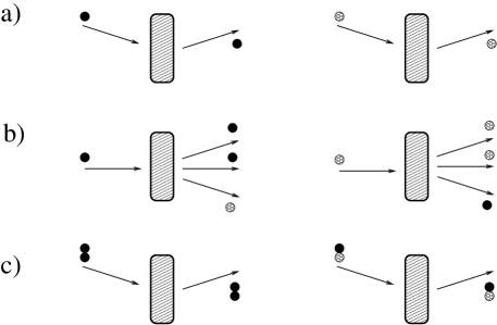
Figure 1: Sketch of possible scattering processes at a two-wire junction (note that incoming particles from wire $j$ can either be scattered into the same wire, or into a different wire):
(a) Single-particle/single-hole scattering processes. These are determined by $H_{\rm tun}$ in Eq. (5) and are fully described in terms of a single-particle $S$-matrix;
(b) Many-body scattering processes in which one particle/one hole is scattered into two particles and one hole/two holes and one particle. These processes can be induced by boundary interaction Hamiltonians such as those in Eq. (6) and their proliferation requires resorting to a bosonic Luttinger-liquid description of the junction;
(c) Scattering processes for a particle-particle and for a particle-hole pair. These are again determined by the Hamiltonians in Eq. (6) and are the only allowed processes in the presence of a strong repulsive (attractive) interaction in the spin (charge) channel, and vice versa. On pertinently defining new fermionic coordinates, they can still be described in terms of a ”single-pair” $S$-matrix.

$$r(D) = \frac{t_{0}\left|D/D_{0}\right|^{-\beta}}{\sqrt{\left|r_{0}\right|^{2}+\left|t_{0}\right|^{2}\left|D/D_{0}\right|^{-2\beta}}}$$

$$t(D) = \frac{t_{0}\left|D/D_{0}\right|^{\beta}}{\sqrt{\left|r_{0}\right|^{2}+\left|t_{0}\right|^{2}\left|D/D_{0}\right|^{2\beta}}}\>\>\>\>,$$ (13)

with $r_{0},t_{0}$ corresponding to the ”bare” scattering amplitudes in Eq. (8). Another case in which an explicit analytical solution can be provided corresponds to having $g_{1\perp}=g_{1\parallel}=g_{1}$ and $g_{2\perp}=g_{2\parallel}=g_{2}$. In this case, the set of Eqs. (73) collapse onto a set of two equations for $g_{1}(D),g_{2}(D)$ which can be readily integrated, yielding the running interaction strengths

$$g_{1}(D) = \frac{g_{1}}{1+\frac{g_{1}}{\pi v}\ln\frac{D_{0}}{D}}$$

$$g_{2}(D) = g_{2}-\frac{g_{1}}{2}+\frac{1}{2}\frac{g_{1}}{1+\frac{g_{1}}{\pi v}\ln\frac{D_{0}}{D}}\>\>\>\>,$$ (14)

and $\beta(D)=[g_{2}(D)-2g_{1}(D)]/(2\pi v)$. Once $\beta(D)$ is known, Eqs. (10) can be integrated, yielding

$$G(D)=\frac{e^{2}}{\pi}\>\left[\frac{T_{0}\left[1+\frac{g_{1}}{\pi v}\ln\left|\frac{D_{0}}{D}\right|\right]^{3/2}\left|D/D_{0}\right|^{2\gamma}}{R_{0}+T_{0}\left[1+\frac{g_{1}}{\pi v}\ln\left|\frac{D_{0}}{D}\right|\right]^{3/2}\left|D/D_{0}\right|^{2\gamma}}\right]\;\;\;\;,$$ (15)

with $\gamma=\left(-\frac{g_{1}}{2}+g_{2}\right)/(2\pi v)$, $T_{0}=|t_{0}|^{2},R_{0}=|r_{0}|^{2}$. As an example of typical scaling plots for $G(D)$ in the simple cases discussed before, in Fig. 2 we plot $G(D)\pi/e^{2}$ vs. $\ln(D_{0}/D)$, as from Eq. (13) (panel (a)) and from Eq. (15) (panel (b)), with the values of the parameters reported in the caption. Consistently with the results obtained within Luttinger liquid framework Furusaki and Nagaosa (1993); Kane and Fisher (1992a, b), $G(D)\pi/e^{2}$ either flows to 0 for an effectively repulsive interaction ($\beta,\gamma>0$), or to 2 (the maximum value allowed by unitarity), for an effectively attractive interaction ($\beta,\gamma<0$). For general values of the interaction strengths, the equations have to be numerically integrated. In Fig. 3, we provide some examples of scaling of $G(D)$ vs. $\ln(D_{0}/D)$ in the general case. It is important to stress Lal et al. (2002) that, due to the nontrivial renormalization group flow of the interaction strengths, the flow of $G(D)$ can be a nonmonotonic function of $D$ for some specific values of the interaction strengths. It would be interesting to check such a feature in a real life two-wire junction: remarkably, this prediction is only obtained within the FRG-approach, in which it is possible to account for the flow of the running interaction strengths, as well.

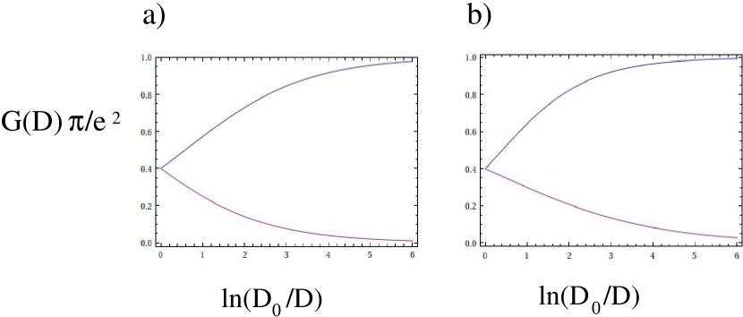
Figure 2: (a) Plot of $G(D)$ vs. $\ln(D_{0}/D)$ as from Eq. (13) for $T_{0}=1-R_{0}=0.4$, $\beta=0.35$ (purple curve - corresponding to an effectively repulsive interaction), and $\beta=-0.35$ (blue curve - corresponding to an effectively attractive interaction), with $T_{0}=|t_{0}|^{2},R_{0}=|r_{0}|^{2}$;
(b) Plot of $G(D)$ vs. $\ln(D_{0}/D)$ as given in Eq. (15) for $T_{0}=1-R_{0}=0.4$, $g_{1}/(2\pi v)=0.2$, $\gamma=0.36$ (purple curve - corresponding to an effectively repulsive interaction), and $\beta=-0.36$ (blue curve - corresponding to an effectively attractive interaction).

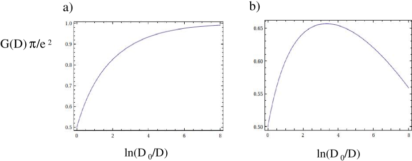
Figure 3: (a) Plot of $G(D)$ vs. $\ln(D_{0}/D)$, obtained by numerically integrating Eqs. (10,11,73) for $g_{1,\parallel}(D_{0})/(2\pi v)=g_{1,\perp}(D_{0})/(2\pi v)=g_{2,\perp}(D_{0})/(2\pi v)=0.3$, $g_{2,\parallel}(D_{0})/(2\pi v)=0$, $R_{0}=T_{0}=0.5$;
(b) Same as in panel ${\bf(a)}$, but with $g_{2,\parallel}(0)/(2\pi v)=0.3$, as well.

The possibility of mapping out the full crossover of the conductance as a function of the scale $D$ is possibly the most important feature of the FRG approach. Yet, since, as we discuss to some extent in Appendix A, the validity of the FRG technique is grounded on the assumption that all the relevant scattering processes at the junction are described by the single-particle $S$-matrix Matveev et al. (1993); Yue et al. (1994); Lal et al. (2002); Nazarov and Glazman (2003), it breaks down when attempting to recover the full crossover of the conductance towards fixed points where multi-particle scattering is the most relevant process at the junction, such as the strongly coupled fixed point stabilized by either $H_{2,0}$ or $H_{0,2}$ in Eq. (6) Furusaki and Nagaosa (1993); Kane and Fisher (1992a, b). Technically, what happens is that, as soon as boundary operators such as $H_{2,0}$ or $H_{0,2}$ become relevant, the proliferation of low-energy many-body scattering processes such as the one we sketch in Fig. 1 (b) invalidates the single-particle $S$-matrix description of the junction dynamics. Nevertheless, some many-body scattering processes can be strongly limited by having, for instance, a strong repulsive interaction among particles with the same spin and a strong attractive interaction among particles with the same charge. In the bosonic framework, this corresponds to having values of the Luttinger parameters in Eqs. (90) such that $g_{c}\geq 2,g_{s}\ll 1$. Indeed, in this limit on one hand, the strong spin repulsive interaction forbids the single-particle processes described by $H_{B}$ in Eq. (5) (at small values of the boundary coupling strengths $\tau_{X,X^{\prime}},\mu_{X,X^{\prime}}$ this can be readily seen from the explicit result for the scaling dimension of $H_{B}$ computed within the bosonization approach, which is $x_{B,weak}=1-\frac{1}{2g_{c}}-\frac{1}{2g_{s}}$, which becomes $\gg 1$, corresponding to a largely irrelevant operator). On the other hand, one expects that the strong charge attraction stabilizes tunneling of composite objects carrying zero spin, such as two-particle pairs, as the one depicted at the left-hand panel of Fig. 1 (c). As a consequence, due to the fact that these are again one-into-one scattering processes, one expects that it is possible to choose the effective low-energy degrees of freedom of the system to resort to a single-particle $S$-matrix in the new coordinates. In fact, this is the idea behind the dual fermion approach we are going to discuss next. When resorting to dual fermion coordinates, an important issue is related to whether the vacuum states at a fixed particle number von Delft and Schoeller (1998) for the original and the dual-fermions are the same. In fact, while dual fermion formalism only captures “composite” excitations e.g. two-particle states in the $g_{c}\sim 2,g_{s}\ll 1$-regime, at such values of the parameters, these states are the only ones that at low energy are effectively able to tunnel across the junction (that is, the only ones whose tunneling is described by a non-irrelevant operator). So, as long as one is only concerned about states relevant for low-energy tunneling across the junction (that is, states relevant for the calculation of the dc-conductance tensor of the junction), one can effectively assume that the fixed-particle number vacuum states are the same in terms of the new (dual) and of the old fermions. The definition of the dual fermion operators strongly depends on the boundary conditions of the various fields at the junction. Accordingly, in the following we define different dual fermion operators in different regimes of values of the boundary interaction, and eventually show that, whenever two different sets of dual coordinates apply to the same region, they yield the same results, as they are expected to.

Let us begin with the weak boundary interaction regime. Referring to the bosonization formulas of Appendix B, this corresponds to assuming Neumann (Dirichlet) boundary conditions for all the $\Phi$ ($\Theta$)-fields in Appendix B and, in addition, to equating the Klein factors so that $\eta_{R,\sigma,j}=\eta_{R,\sigma,j}$, $\forall\sigma,j$. In this limit, one may respectively rewrite $H_{0,2}$ and $H_{2,0}$ in bosonic coordinates as

$$H_{2,0} = v_{2,0}\cos[\Phi_{1,c}(0)-\Phi_{2,c}(0)]$$

$$H_{0,2} = v_{0,2}\cos[\Phi_{1,s}(0)-\Phi_{2,s}(0)]\>\>\>\>,$$ (16)

with $v_{2,0}\propto V_{2,0},v_{0,2}\propto V_{0,2}$. The scaling dimensions of the operators in Eqs. (16) are respectively given by $x_{2,0}=2/g_{c},x_{0,2}=2/g_{s}$. Thus, in the regime of a strongly attractive interaction in the charge (spin)-channel and strongly repulsive interaction in the spin (charge)-channel, $H_{2,0}$ ($H_{0,2}$) may become the most relevant boundary operator at weak boundary coupling. The strategy of our dual fermion approach consists in defining a novel set of fermionic fields, in terms of which the operators in Eqs. (16) are realized as bilinears, similar to the $B$-operators in Eq. (4). To be specific, let us introduce the center-of-mass and the relative fields in the charge- and in the spin-sector, respectively given by

$$\Phi_{c(s)}(x) = \frac{1}{\sqrt{2}}[\Phi_{1,c(s)}(x)+\Phi_{2,c(s)}(x)]$$

$$\Theta_{c(s)}(x) = \frac{1}{\sqrt{2}}[\Theta_{1,c(s)}(x)+\Theta_{2,c(s)}(x)]\>\>\>\>,$$ (17)

and

$$\varphi_{c(s)}(x) = \frac{1}{\sqrt{2}}[\Phi_{1,c(s)}(x)-\Phi_{2,c(s)}(x)]$$

$$\vartheta_{c(s)}(x) = \frac{1}{\sqrt{2}}[\Theta_{1,c(s)}(x)-\Theta_{2,c(s)}(x)]\>\>\>\>.$$ (18)

Next, let us perform the canonical transformation to a new set of bosonic fields, defined as

$$\left[\begin{array}[]{c}\bar{\Phi}_{c(s)}(x)\\ \bar{\Theta}_{c(s)}(x)\\ \bar{\varphi}_{c(s)}(x)\\ \bar{\vartheta}_{c(s)}(x)\end{array}\right]=\left[\begin{array}[]{cccc}\sqrt{2}&0&0&0\\ 0&\frac{1}{\sqrt{2}}&0&0\\ 0&0&\sqrt{2}&0\\ 0&0&0&\frac{1}{\sqrt{2}}\end{array}\right]\left[\begin{array}[]{c}\Phi_{c(s)}(x)\\ \Theta_{c(s)}(x)\\ \varphi_{c(s)}(x)\\ \vartheta_{c(s)}(x)\end{array}\right]\>\>\>\>.$$ (19)

It is worth stressing that the transformation in Eqs. (19) relate to each other bosonic operators at a given position in real space. Since the correspondence rules between the bosonic and the (original or dual) fermionic fields, summarized in Appendix B, are local in real space, as well, one concludes that, written in terms of dual fermionic coordinates, the boundary interaction Hamiltonian $H_{B}$ is still local and that the dynamics far from the junction can be fully encoded within dual fermion scattering states. Now, assuming $g_{s}\ll 1$, $g_{c}=2+\delta g_{c}$, with $|\delta g_{c}|\ll 1$, we see that $g_{s}\ll 1$ makes $H_{0,2}$ strongly irrelevant. This fully suppresses spin transport across the junction and, therefore, we may just focus onto charge transport, ruled by $H_{2,0}$. In fact, it appears that single-spinful particle-tunneling processes are already suppressed against two-particle pair tunneling processes as soon as $g_{s}<2/3$. As conservation of spin symmetry implies $g_{s}=1$, in order to realize the condition above one may, for instance, think of two coupled spinless interacting one-dimensional electronic systems (which could possibly realized as semiconducting quantum wires in the presence of spin-orbit and Zeeman interactions), with a mismatch in the Fermi momenta that prevents the interaction from opening a gap in the fermion spectrum. The two channels can, therefore, be regarded as the two opposite spin polarization, although without any symmetry implying $g_{s}=1$. To rewrite this latter operator as a bilinear functional of fermionic operators, we define the spinless chiral fermionic fields $\chi_{R,j}(x),\chi_{L,j}(x)$ as

$$\chi_{R,j}(x) = \eta_{R,j}\;e^{\frac{i}{2}[\bar{\Phi}_{c}(x)-(-1)^{j}\bar{\varphi}_{c}(x)+\bar{\Theta}_{c}(x)-(-1)^{j}\bar{\vartheta}_{c}(x)]}$$

$$\chi_{L,j}(x) = \eta_{L,j}\;e^{\frac{i}{2}[\bar{\Phi}_{c}(x)+(-1)^{j}\bar{\varphi}_{c}(x)+\bar{\Theta}_{c}(x)+(-1)^{j}\bar{\vartheta}_{c}(x)]}\;\;\;\;,$$ (20)

with $j=1,2$ and with $\eta_{R,j},\eta_{L,j}$ being real fermionic Klein factors. ”Inverting” the bosonization procedure outlined in Appendix B into a pertinent re-fermionization to spinless fermions, we find that the bulk Hamiltonian for the $\chi$-fermions is given by

$$H_{\rm c;bulk} = -iu\sum_{j=1,2}\;\int_{0}^{L}\;dx\;\{\chi_{R,j}^{\dagger}(x)\partial_{x}\chi_{R,j}(x)-\chi_{L,j}^{\dagger}(x)\partial_{x}\chi_{L,j}(x)\}$$

$$- \frac{u\pi\delta g_{c}}{2} \sum_{j=1,2}\;\int_{0}^{L}\;dx\;:\chi_{R,j}^{\dagger}(x)\chi_{R,j}(x)::\chi_{L,j}^{\dagger}(x)\chi_{L,j}(x):\;\;\;\;,$$ (21)

with the velocity $u\propto v$. The $\chi_{L/R,j}$-fields are the appropriate degrees of freedom to describe pair scattering at the junction in terms of a single-particle $S$-matrix. In order to prove that it is so, we note that $H_{2,0}$ can be regarded as the bosonic expression for the boundary weak coupling limit of a tunnel Hamiltonian for the spinless fermions, $H_{\rm c,tun}$, given by

$$H_{\rm c,tun}=v_{2,0}\{\chi_{1}^{\dagger}(0)\chi_{2}(0)+\chi_{2}^{\dagger}(0)\chi_{1}(0)\}\;\;\;\;,$$ (22)

with $\chi_{j}(0)=\chi_{R,j}(0)+\chi_{L,j}(0)$. While the strong spin repulsion sets the spin conductance tensor to 0, the charge conductance can nevertheless be different from zero, due to zero-spin pair-tunneling across the junction. Once the RG-flow for the $S$-matrix elements describing $\chi$-fermion scattering at the junction has been derived as we did before, using the formulas we report in Appendix C.1 and the expression of the charge current operator in wire $j$ in terms of the dual fermionic fields:

$$J_{c,j}(x)=eu\sqrt{2}\>\{:\chi_{R,j}^{\dagger}(x)\chi_{R,j}(x):-:\chi_{L,j}^{\dagger}(x)\chi_{L,j}(x):\}\>\>\>\>,$$ (23)

we obtain that the charge conductance tensor scales according to

$$G_{c}(D)=\left[\begin{array}[]{cc}\frac{e^{2}}{\pi}-G(D)&G(D)\\ G(D)&\frac{e^{2}}{\pi}-G(D)\end{array}\right]\;\;\;\;,$$ (24)

with

$$G(D)=\frac{e^{2}}{\pi}\>\left[\frac{T_{0}|D/D_{0}|^{-\frac{\delta g_{c}}{2}}}{R_{0}+T_{0}|D/D_{0}|^{-\frac{\delta g_{c}}{2}}}\right]\>\>\>\>,$$ (25)

and the bare reflection and transmission coefficients respectively given by

$$R_{0} = \left|\frac{u^{2}-v_{2,0}^{2}}{u^{2}+v_{2,0}^{2}}\right|^{2}$$

$$T_{0} = \left|\frac{2uv_{2,0}}{u^{2}+v_{2,0}^{2}}\right|^{2}\>\>\>\>.$$ (26)

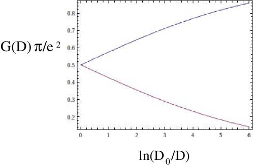
Figure 4: Plot of $G_{c}(D)$ vs. $\ln(D_{0}/D)$ as from Eq. (25) for $T_{0}=R_{0}=0.5$ and for $\delta g_{c}$ respectively equal to 0.6 (blue curve) and to -0.6 (purple curve).

In Fig. 4, we plot $G(D)$ versus $\ln(D_{0}/D)$ in two paradigmatic cases, respectively corresponding to $\delta g_{c}>0$ and to $\delta g_{c}<0$. To our knowledge, this is the first example of a full scaling plot of the conductance for a junction of strongly interacting one-dimensional quantum wires. While, on one hand, this shows the effectiveness of our approach in describing the crossover of the conductance towards the spin-insulating charge-conducting fixed point, on the other hand, one has also to prove the consistency of an effective theory strongly relying on the weak boundary coupling assumption with an RG-flow taking the system all the way down to the perfectly charge-conducting fixed point, corresponding to the strongly interacting limit of the boundary interaction Furusaki and Nagaosa (1993); Kane and Fisher (1992a, b). When $\delta g_{c}>0$, the relevance of $H_{2,0}$ drives the system towards the strongly boundary interaction limit in the charge channel, corresponding to pinning $\varphi_{c}(0)$ and, accordingly, to imposing Neumann boundary conditions on $\vartheta_{c}(0)$. Since $\Phi_{c}(0)$ does not appear in the boundary interaction, one assumes that it still obeys Neumann boundary conditions and, accordingly, that $\Theta_{c}(0)$ is pinned at a constant value. We now prove that these boundary conditions are recovered by taking the strongly coupled limit of $H_{\rm c,tun}$ in Eq. (22) and using the refermionization rules in Eqs. (20). Indeed, on making the strong-coupling assumption, $\left|\frac{v_{2,0}}{u}\right|\gg 1$, as from Eqs. (26), one obtains $R_{0}\to 0,T_{0}\to 1$, that is, the boundary conditions correspond to perfect transmission from wire-1 to wire-2, and vice versa. In terms of the dual fermionic fields, this corresponds to the conditions

$$\chi_{R,2}(x) = e^{i\lambda}\>\chi_{L,1}(-x)$$

$$\chi_{R,1}(x) = e^{-i\lambda}\>\chi_{L,2}(-x)\;\;\;\;,$$ (27)

with $\lambda$ being some nonuniversal phase. From Eqs. (20), one sees that Eqs. (27) imply Dirichlet boundary conditions at $x=0$ for both $\bar{\varphi}_{c}(x)$ and $\bar{\Theta}_{c}(x)$, with the dual fields $\bar{\vartheta}_{c}(x),\bar{\Phi}_{c}(x)$ obeying Neumann boundary conditions. This is exactly the same result one would obtain working in bosonic variables by sending to $\infty$ the interaction strength $v_{2,0}$ in Eq. (16). Due to the strong repulsion in the spin channel, such a fixed point corresponds to perfect transmission in the charge channel, but perfect reflection in the spin channel, that is, it must be identified with the non-symmetric charge-conducting spin-insulating phase of Refs. [Furusaki and Nagaosa, 1993; Kane and Fisher, 1992a, b]. To conclude the consistency check, we note that, on alledging for additional backscattering contributions to $H_{c,tun}$ of the generic form $\mu_{1}\chi_{R,1}^{\dagger}(0)\chi_{R,1}^{\dagger}(0)+\mu_{2}\chi_{L,1}^{\dagger}(0)\chi_{L,}^{\dagger}(0)$ (which play no role at weak coupling) and using again Eqs. (27), one obtains the bosonic operators

$$\tilde{H}_{\rm c,tun}\sim\mu\cos\left[\bar{\vartheta}_{c}(0)\right]\>\>\>\>,$$ (28)

with $\mu$ being some nonuniversal constant. Equation (28) corresponds to the bosonic version of the leading boundary perturbation at the non-symmetric charge-conducting spin-insulating fixed point Furusaki and Nagaosa (1993); Kane and Fisher (1992a, b).

Our approach also allows for analyzing the complementary situation in which $g_{c}\ll 1$ and $g_{s}\sim 2$. In this case, one expects that the strong repulsion in the charge channel and the strong attraction in the spin channel stabilize single-pair tunneling processes at the junction such as those sketched at the right-hand panel of Fig. 1 (c), that is, tunneling of particle-hole pairs, with total spin 1. Again, for $g_{s}=2$, the $S$-matrix describes single-particle into single-particle scattering processes, once it is written in the appropriate basis. To select the pertinent degrees of freedom, we therefore repeat the refermionization procedure in Eq. (20), by just exchanging the charge- and the spin-sector with each other. Of course, charge- and spin-conductance are exchanged with each other, compared to the previous situation and, accordingly, the flow will be towards the charge-insulating spin-conducting fixed point of Refs. [Furusaki and Nagaosa, 1993; Kane and Fisher, 1992a, b]. An important remark, however, concerns the effects of a possible residual interaction, which, as we did before, can be in principle introduced for accounting for $g_{s}$ slightly different from 2. Indeed, a term in the ”residual” bulk interaction Hamiltonian such as the one $\propto g_{j,1,\perp}$ in Eq. (2), once expressed in terms of the fermionic fields in Eqs. (20) would take the form

$$H_{\delta}=\sum_{j=1}^{2}\>m_{j}\>\int\>dx\>\{\chi_{R,j}^{\dagger}(x)\chi_{L,j}(x)+\chi_{L,j}^{\dagger}(x)\chi_{R,j}(x)\}\>\>\>\>,$$ (29)

with $m_{j}\propto g_{j,1,\perp}$, which would open a bulk gap in the single-$\chi$ fermion spectrum, thus making the whole system behave as a bulk spin insulator. Therefore, in order to recover the correct physics of the charge-insulating spin-conducting fixed point, we must assume that all the $g_{j,1,\perp}$ are tuned to zero, which is typically the case when resorting to the bosonic approach to spinful electrons Furusaki and Nagaosa (1993); Kane and Fisher (1992a, b).

As we have just shown, resorting to pertinent dual-fermion operators allows for mapping out the full crossover with the appropriate energy scale of the charge and/or spin conductance of a junction in region of values of the interaction parameters in which one is typically forbidden to use the standard weak-coupling formulation of either FRG, or fRG. In the following, we apply our technique to the spinful three-wire junction studied using the bosonization approach in Ref. [Hou and Chamon, 2008], and will recover the full crossover of the conductance tensor in regions typically not accessible in the bosonic formalism.

III Dual Fermionic variables and renormalization group approach to the calculation of the conductance at a junction of three spinful interacting quantum wires

We now consider a three-spinful-wire junction, such as the one we sketch in Fig. 5. Resorting to the appropriate fermionic variables, we generalize to strongly interacting regions the weak-coupling FRG-approach. As a result, we map out the full dependence of the conductance tensor on the low-energy running cutoff scale even in strongly-interacting regions of the parameter space. Eventually, we discuss the consistency of our results about the phase diagram of the junction with those obtained in Ref. [Hou and Chamon, 2008], particularly showing how our technique can be used to recover informations that typically cannot be derived within the bosonization approach used there. Consistently with Ref. [Hou and Chamon, 2008], in the following, we make the simplifying assumption that, in the weakly interacting regime, the bulk interaction is purely intra-wire and is the same in all the three wires. In fact, while this assumption is already expected to yields quite a rich phase diagram Hou and Chamon (2008), in principle our approach can be readily generalized to cases of different bulk interactions in different wires, such as the one considered in Ref. [Hou et al., 2012].

Figure 5: Sketch of a three-wire junction of spinful quantum wires pierced by a magnetic flux $\Phi$.

III.1 The weakly interacting regime

For a weak boundary interaction, assuming total spin conservation at the junction, the most relevant boundary interaction Hamiltonian is a combination of the bilinear operators in Eq. (4). The relevant scattering processes at the junction are all encoded in the single-particle $S$-matrix elements, $S_{(j,\sigma),(j^{\prime},\sigma^{\prime})}(k)$. Because of spin conservation, the $S$-matrix is diagonal in the spin index, that is, $S_{(j,\sigma),(j^{\prime},\sigma^{\prime})}(k)=\delta_{\sigma,\sigma^{\prime}}S_{j,j^{\prime}}(k)$. Assuming also that the boundary Hamiltonian is symmetric under exchanging the wires with each other, the $3\times 3$ matrix $S(k)$ takes the form

$$S=\left[\begin{array}[]{ccc}r&\bar{t}&t\\ t&r&\bar{t}\\ \bar{t}&t&r\end{array}\right]\>\>\>\>.$$ (30)

(Note that, in Eq. (30) we assume that all the amplitudes are computed at the Fermi level and accordingly drop the index $k$ from the $S$-matrix elements. This is consistent with the discussion of Appendix A, where we assume that, close to the Fermi level, the scattering amplitudes are smooth functions of $k$.) It is worth mentioning that, in writing Eq. (30), we allowed for time-reversal symmetry breaking as a consequence, for instance, of a magnetic flux $\phi$ piercing the centre of the junction (see Fig. 5). This implies that, in general, the scattering amplitude $t$ from wire $j$ to wire $j+1$ is different from the one from wire $j$ to wire $j-1$ ($\bar{t}$). From Eq. (30) one therefore finds that the $F$-matrix elements in Eq. (71) are given by $F_{j,j^{\prime}}=\frac{\beta}{2}r\delta_{j,j^{\prime}}$, with again $\beta=\frac{1}{2\pi v}\left[-g_{1\parallel}-g_{1\perp}+g_{2\parallel}\right]$. On applying the FRG formalism of Appendix A, one readily obtains the RG-equations for the independent $S$-matrix elements, given by

$$\frac{dr}{d\ell} = \frac{\beta}{2}\left[r-\left|r\right|^{2}r-2t\bar{t}r^{*}\right]$$

$$\frac{dt}{d\ell} = -\frac{\beta}{2}\left[2t\left|r\right|^{2}+\bar{t}^{2}r^{*}\right]$$

$$\frac{d\bar{t}}{d\ell} = -\frac{\beta}{2}\left[2\bar{t}\left|r\right|^{2}+t^{2}r^{*}\right]\>\>\>\>,$$ (31)

which, again, must be supplemented with the RG-equations for the running coupling strengths, Eqs. (73,11). Since, as a consequence of spin conservation in scattering processes at the junction, the $S$-matrix is diagonal in the spin indices, the charge- and spin-conductance tensors are equal to each other at the fixed points, as well as along the RG-trajectories obtained integrating Eqs. (31). In particular, using the formalism of Appendix C.1, one obtains

$$G_{c,s}(D)=\frac{e^{2}}{\pi}\left[\begin{array}[]{ccc}-R(D)+1&-\bar{T}(D)&-T(D)\\ -T(D)&-R(D)+1&-\bar{T}(D)\\ -\bar{T}(D)&-T(D)&-R(D)+1\end{array}\right]\;\;\;\;,$$ (32)

with $R(D)=|r(D)|^{2},T(D)=|t(D)|^{2}$, and $\bar{T}(D)=|\bar{t}(D)|^{2}$. The RG-flow of the scattering coefficients $T(D),\bar{T}(D)$ is recovered by solving the set of differential equations

$$\frac{dT}{d\ell} = -\frac{\beta}{2}\left[\left(5T-\bar{T}\right)(1-T-\bar{T})-T\bar{T}\right]$$

$$\frac{d\bar{T}}{d\ell} = -\frac{\beta}{2}\left[\left(5\bar{T}-T\right)(1-T-\bar{T})-T\bar{T}\right]\;\;\;\;,$$ (33)

which are derived from Eqs. (31) by taking into account the unitarity constraint $T(D)+\bar{T}(D)+R(D)=1$. The fixed points of the boundary phase diagram are, therefore, determined by setting to zero the terms at the right-hand side of Eqs. (33). From Eq. (32) one may therefore recover the corresponding charge- and the spin-conductance tensors. Borrowing the labels used in Ref. [Hou and Chamon, 2008], we obtain the following fixed points:

• The $[N_{c},N_{s}]$ (”disconnected”) fixed point

  This fixed point corresponds to having $R=1$ and $T=\bar{T}=0$ which, according to Eq. (32), yields

  $$G_{c}=G_{s}=\frac{e^{2}}{\pi}\left[\begin{array}[]{ccc}0&0&0\\ 0&0&0\\ 0&0&0\end{array}\right]\>\>\>\>,$$ (34)

  as it is appropriate for a disconnected junction.

• The $\chi_{++}$ fixed point

  This corresponds to $R=\bar{T}=0$, $T=1$, which yields

  $$|S_{j,j^{\prime}}|^{2}=\left[\begin{array}[]{ccc}0&0&1\\ 1&0&0\\ 0&1&0\end{array}\right]\>\>\>\>,$$ (35)

  and, accordingly

  $$G_{c}=G_{s}=\frac{e^{2}}{\pi}\left[\begin{array}[]{ccc}1&0&-1\\ -1&1&0\\ 0&-1&1\end{array}\right]\>\>\>\>;$$ (36)

• The $\chi_{--}$ fixed point

  This corresponds to $R=T=0$, $\bar{T}=1$, which yields

  $$|S_{j,j^{\prime}}|^{2}=\left[\begin{array}[]{ccc}0&1&0\\ 0&0&1\\ 1&0&0\end{array}\right]\>\>\>\>,$$ (37)

  and, accordingly

  $$G_{c}=G_{s}=\frac{e^{2}}{\pi}\left[\begin{array}[]{ccc}1&-1&0\\ 0&1&-1\\ -1&0&1\end{array}\right]\>\>\>\>;$$ (38)

• The $M$ fixed point

  This corresponds to $T=\bar{T}=\frac{4}{9}$, $R=\frac{1}{9}$ and has to be identified with the symmetric Lal et al. (2002), or with the Griffith Das et al. (2008) fixed point of a junction of three interacting wires. One obtains

  $$|S_{j,j^{\prime}}|^{2}=\left[\begin{array}[]{ccc}\frac{1}{9}&\frac{4}{9}&\frac{4}{9}\\ \frac{4}{9}&\frac{1}{9}&\frac{4}{9}\\ \frac{4}{9}&\frac{4}{9}&\frac{1}{9}\end{array}\right]\>\>\>\>,$$ (39)

  and, accordingly

  $$G_{c}=G_{s}=\frac{e^{2}}{\pi}\left[\begin{array}[]{ccc}\frac{8}{9}&-\frac{4}{9}&-\frac{4}{9}\\ -\frac{4}{9}&\frac{8}{9}&-\frac{4}{9}\\ -\frac{4}{9}&-\frac{4}{9}&\frac{8}{9}\end{array}\right]\>\>\>\>.$$ (40)

$\chi_{\pm\pm}$ must clearly be identified with the ”chiral” fixed points of Ref. [Hou and Chamon, 2008], where time-reversal symmetry breaking is maximum, both in the charge and in the spin sector. Along the RG-trajectories connecting two fixed points, the conductance flow is determined by Eq. (32). The topology and the direction of the RG-trajectories depend on both $\beta$ and on the bare values of the $S$-matrix elements. $\beta$ scales with $\ell$ as determined by Eqs. (73,11), which makes it necessary to resort to a full numerical integration approach. A set of simplified situations can be realized, however, where $\beta$ keeps constant along RG-trajectories. For instance, if $g_{1,\perp}(D_{0})=0$, Eq. (11) implies that $\beta$ is constant. In this case, from Eqs. (33) one readily sees that, if $\beta>0$, the boundary flow is towards the $NN$-fixed point. At variance, if $\beta<0$ and $T(D_{0})>(<)\bar{T}(D_{0})$, the boundary flow is towards the $\chi_{++}$ ($\chi_{--}$)-fixed point. As an example of possible RG-trajectories that may be realized in this specific case, in Fig. 6 we plot $T(D)$ and $\bar{T}(D)$ for $\beta$ constant and negative, while we draw similar plots in Fig. 7 for constant and positive $\beta$ and in Fig. 8 for non-constant $\beta$ (see the captions for details).

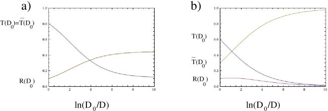
Figure 6: Renormalization group flow of the scattering coefficients for a three-wire junction for $g_{1,\perp}=0$, $\beta$ constant and equal to -0.3, and different choices of the initial values of the scattering coefficients:
(a) Renormalization group flow corresponding to $T(D_{0})=\bar{T}(D_{0})=0.1$, $R(D_{0})=0.8$. The curves corresponding to $T(D)$ and to $\bar{T}(D)$ vs $\ln(D_{0}/D)$ collapse onto the single red curve of the graph, while the flow of $R(D)$ vs $\ln(D_{0}/D)$ is described by the blue curve. As $D_{0}/D$ grows, the scattering coefficients flow towards the asymptotic values corresponding to the $M$-fixed point;
(b) Renormalization group flow corresponding to $T(D_{0})=0.1,\bar{T}(D_{0})=0.3,R(D_{0})=0.6$. As $D_{0}/D$ grows, the scattering coefficients flow towards the asymptotic values corresponding to the $\chi_{--}$-fixed point.

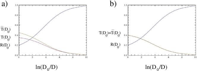
Figure 7: Renormalization group flow of the scattering coefficients for a three-wire junction for $g_{1,\perp}=0$, $\beta$ constant and equal to 0.3, and different choices of the initial values of the scattering coefficients:
(a) Renormalization group flow corresponding to $T(D_{0})=0.35,\bar{T}(D_{0})=0.45,R(D_{0})=0.2$;
(b) Renormalization group flow corresponding to $T(D_{0})=\bar{T}(D_{0})=0.4,R(D_{0})=0.2$. As $D_{0}/D$ grows, in both cases the scattering coefficients flow towards the $NN$-fixed point.

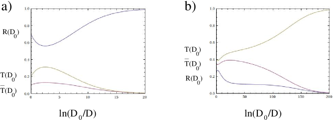
Figure 8: Renormalization group flow of the scattering coefficients for a three-wire junction for non-constant $\beta$:
(a) Renormalization group flow corresponding to $T(D_{0})=0.2,\bar{T}(D_{0})=0.1,R(D_{0})=0.4$ and to $g_{1,\parallel}(D_{0})/(2\pi v)=g_{1,\perp}(D_{0})/(2\pi v)=g_{2,\parallel}(D_{0})/(2\pi v)=g_{1,\perp}(D_{0})/(2\pi v)=0.4$. For these values of the bare parameters the junction is attracted by the disconnected fixed point ($R\to 1$ while $T,\bar{T}\to 0$);
(b) Renormalization group flow corresponding to $T(D_{0})=0.4,\bar{T}(D_{0})=0.35,R(D_{0})=0.25$ and to $g_{1,\parallel}(D_{0})/(2\pi v)=0.3,g_{1,\perp}(D_{0})/(2\pi v)=-0.2,g_{2,\parallel}(D_{0})/(2\pi v)=g_{1,\perp}(D_{0})/(2\pi v)=0.2$. For these values of the bare parameters the junction is attracted by the $\chi_{++}$-fixed point.

All the analysis we have done so far applies to a junction of three spinful quantum wires for weak bulk interaction. We now employ the dual-fermion approach to generalize the FRG-technique to regimes corresponding to strong bulk interactions either in the charge-, or in the spin-channel (or in both of them).

III.2 Fermionic analysis of the strongly interacting regime at $g_{c}\sim g_{s}\sim 3$

A first regime to which our dual-fermion approach can be successfully applied corresponds to a strong attractive interaction, both in the charge and in the spin channels. In particular, we assume $g_{c}\sim g_{s}\sim 3$. According to the phase diagram derived in Ref. [Hou and Chamon, 2008] within the bosonization approach, in this range of values of the Luttinger parameters one expects to find a fixed point where paired electron tunneling and Andreev reflection are the dominant scattering processes at the junction and, in addition, two fixed points with maximally broken time-reversal symmetry, to be identified with the $\chi_{++}$ and the $\chi_{--}$-fixed points discussed in the previous subsection. To apply the FRG-approach to this part of the phase diagram, we have to define the appropriate dual fermion coordinates. To do so, let us set $g_{c}=g_{s}=3$. We therefore note that, though, in general, the charge- and spin-velocities $u_{c}$ and $u_{s}$ can be different from each other, one may easily make them equal by a pertinent rescaling of the real-space coordinate in the charge- and in the spin-sector of the bosonic Hamiltonian in Eq. (89). As the rescaling does not affect the boundary interaction (which is localized at $x=0$), in the following, without loss of generality, we will assume $u_{c}=u_{s}\equiv u$. In choosing the appropriate dual fermion coordinates, we use the criterion of mapping the fixed point we recover in the strongly interacting limit one-to-one onto those of the phase diagram in the weakly interacting regime. Referring to the bosonization formulas of Appendix B, we define the dual bosonic fields $\tilde{\Phi}_{c(s),j}(x),\tilde{\Theta}_{c(s),j}(x)$ in terms of those in Eqs. (80,81) as

$$\left[\begin{array}[]{c}\tilde{\Phi}_{c(s),1}(x)\\ \tilde{\Phi}_{c(s),2}(x)\\ \tilde{\Phi}_{c(s),3}(x)\\ \tilde{\Theta}_{c(s),1}(x)\\ \tilde{\Theta}_{c(s),2}(x)\\ \tilde{\Theta}_{c(s),3}(x)\end{array}\right]=\left[\begin{array}[]{cccccc}\frac{1}{\sqrt{3}}&\frac{1}{\sqrt{3}}&\frac{1}{\sqrt{3}}&0&\frac{1}{3}&-\frac{1}{3}\\ \frac{1}{\sqrt{3}}&\frac{1}{\sqrt{3}}&\frac{1}{\sqrt{3}}&-\frac{1}{3}&0&\frac{1}{3}\\ \frac{1}{\sqrt{3}}&\frac{1}{\sqrt{3}}&\frac{1}{\sqrt{3}}&\frac{1}{3}&-\frac{1}{3}&0\\ 0&-1&1&\frac{1}{3\sqrt{3}}&\frac{1}{3\sqrt{3}}&\frac{1}{3\sqrt{3}}\\ 1&0&-1&\frac{1}{3\sqrt{3}}&\frac{1}{3\sqrt{3}}&\frac{1}{3\sqrt{3}}\\ -1&1&0&\frac{1}{3\sqrt{3}}&\frac{1}{3\sqrt{3}}&\frac{1}{3\sqrt{3}}\\ \end{array}\right]\left[\begin{array}[]{c}\Phi_{c(s),1}(x)\\ \Phi_{c(s),2}(x)\\ \Phi_{c(s),3}(x)\\ \Theta_{c(s),1}(x)\\ \Theta_{c(s),2}(x)\\ \Theta_{c(s),3}(x)\end{array}\right]\>\>\>\>.$$ (41)

Consistently with Eqs. (83), we therefore define the dual fermionic fields as

$$\tilde{\psi}_{R,\sigma,j}(x) = \eta_{R,\sigma,j}e^{\frac{i}{2}[\tilde{\Phi}_{j,c}(x)+\tilde{\Theta}_{j,c}(x)+\sigma(\tilde{\Phi}_{j,s}(x)+\tilde{\Theta}_{j,s}(x))]}$$

$$\tilde{\psi}_{L,\sigma,j}(x) = \eta_{L,\sigma,j}e^{\frac{i}{2}[\tilde{\Phi}_{j,c}(x)-\tilde{\Theta}_{j,c}(x)+\sigma(\tilde{\Phi}_{j,s}(x)-\tilde{\Theta}_{j,s}(x))]}\;\;\;\;.$$ (42)

Using Eq. (41) one sees that, when expressed in terms of the $\tilde{\Phi}$ and of the $\tilde{\Theta}$-fields, the bulk Hamiltonian in Eq. (89) reduces back to the one with $g_{c}=g_{s}=1$, which, when expressed in terms of the fermionic fields defined in Eqs. (42), corresponds to the free Hamiltonian $H_{0,F}$, given by

$$H_{0,F}=-iu\>\sum_{j=1}^{3}\>\sum_{\sigma}\>\int_{0}^{L}\>dx\>\left\{\tilde{\psi}_{R,j,\sigma}^{\dagger}(x)\partial_{x}\tilde{\psi}_{R,j,\sigma}(x)-\tilde{\psi}_{L,j,\sigma}^{\dagger}(x)\partial_{x}\tilde{\psi}_{L,j,\sigma}(x)\right\}\>\>\>\>.$$ (43)

Equation (43) is the striking result of our technique of introducing dual fermion operators: it is a free-fermion Hamiltonian which describes a system that is strongly interacting in the original coordinates. Based upon the dual fermion fields in Eqs. (42) one may therefore introduce dual boundary operators analogous to those defined in Eq. (4), namely, one may set

$$\tilde{B}_{(j,j^{\prime}),\sigma,(X,X^{\prime})}(0)=\tilde{\psi}_{X,j,\sigma}^{\dagger}(0)\tilde{\psi}_{X^{\prime},j^{\prime},\sigma}(0)\>\>\>\>,$$ (44)

and assume that the boundary interaction is realized as a linear combination of the operators in Eq. (44) and/or of products of two of them. In the absence of additional bulk interaction involving the dual fermion fields, or in the weakly interacting regime, the most relevant boundary interaction term is realized as a linear combination of the $\tilde{B}$-operators only. Therefore, the physically relevant processes at the junction are all encoded within the single-particle $S$-matrix elements in the basis of the dual fields, $\tilde{S}_{(j,\sigma);(j^{\prime},\sigma^{\prime})}$. A nontrivial flow for the $\tilde{S}$-matrix elements is induced by a nonzero bulk interaction in the dual-fermion theory, that is, by having $g_{c(s)}=3+\delta g_{c(s)}$, with $|\delta g_{c(s)}|/g_{c(s)}\ll 1$. The dual interaction Hamiltonian, $\tilde{H}_{\rm int}$ can be readily recovered using Eqs. (41,42). The result is

$$\tilde{H}_{\rm int}=\sum_{j=1}^{3}\>\sum_{\sigma,\sigma^{\prime}}\>g_{j;(\sigma,\sigma^{\prime})}\>\int_{0}^{L}\>dx\>\tilde{\rho}_{R,j,\sigma}(x)\tilde{\rho}_{L,j,\sigma^{\prime}}(x)\>+\sum_{j\neq j^{\prime}=1}^{3}\>\sum_{\sigma,\sigma^{\prime}}\>g_{(j,j^{\prime});(\sigma,\sigma^{\prime})}\>\int_{0}^{L}\>dx\>\tilde{\rho}_{R,j,\sigma}(x)\tilde{\rho}_{L,j^{\prime},\sigma^{\prime}}(x)\>\>\>\>,$$ (45)

with $\tilde{\rho}_{R(L),j,\sigma}(x)=:\tilde{\psi}^{\dagger}_{R(L),j,\sigma}(x)\tilde{\psi}_{R(L),j,\sigma}(x):$, and

$$g_{j;(\sigma,\sigma^{\prime})} = \frac{2\pi u(\delta g_{c}+\delta g_{s})}{9}\delta_{\sigma,\sigma^{\prime}}+\frac{2\pi u(\delta g_{c}-\delta g_{s})}{9}\delta_{\sigma,\bar{\sigma}^{\prime}}$$

$$g_{(j,j^{\prime});(\sigma,\sigma^{\prime})} = -\frac{8\pi u(\delta g_{c}+\delta g_{s})}{9}\delta_{\sigma,\sigma^{\prime}}-\frac{8\pi u(\delta g_{c}-\delta g_{s})}{9}\delta_{\sigma,\bar{\sigma}^{\prime}}\>\>\>\>,$$ (46)

plus terms that do not renormalize the scattering amplitudes. $\tilde{H}_{\rm int}$ takes the form of the generalized bulk Hamiltonian in Eqs. (76,77). Given the corresponding $F$-matrix elements reported in Eq. (79), one may derive the RG-equations in the case in which the spin is conserved at a scattering process at the junction, which implies $\tilde{S}_{(j,\sigma);(j^{\prime},\sigma^{\prime})}=\delta_{\sigma,\sigma^{\prime}}\tilde{S}_{j,j^{\prime}}$, and the boundary interaction is symmetric under a cyclic permutation of the three wires, that is, the $\tilde{S}_{j,j^{\prime}}$-matrix elements are given by

$$\tilde{S}=\left[\begin{array}[]{ccc}\tilde{r}&\tilde{\bar{t}}&\tilde{t}\\ \tilde{t}&\tilde{r}&\tilde{\bar{t}}\\ \tilde{\bar{t}}&\tilde{t}&\tilde{r}\end{array}\right]\>\>\>\>.$$ (47)

Summing over both the inter-wire and the intra-wire processes allowed by the bulk interaction, one obtains

$$\frac{d\tilde{r}}{d\ell} = \left(\frac{\gamma-\alpha}{2}\right)\{\tilde{r}-|\tilde{r}|^{2}\tilde{r}-2\tilde{t}\tilde{\bar{t}}\tilde{r}^{*}\}$$

$$\frac{d\tilde{t}}{d\ell} = -\left(\frac{\gamma-\alpha}{2}\right)\{2\tilde{t}|\tilde{r}|^{2}+(\tilde{\bar{t}})^{2}\tilde{r}^{*}\}$$

$$\frac{d\tilde{\bar{t}}}{d\ell} = -\left(\frac{\gamma-\alpha}{2}\right)\{2\tilde{\bar{t}}|\tilde{r}|^{2}+(\tilde{t})^{2}\tilde{r}^{*}\}\>\>\>\>,$$ (48)

with $\alpha=g_{(j,j^{\prime});(\sigma,\sigma)}/(2\pi u),\gamma=g_{j;(\sigma,\sigma)}/(2\pi u)$. Equations (48) are equal with Eqs. (31) in the weakly interacting case, provided one substitutes the (running) parameter $\beta$ in Eqs. (31) with the (constant) parameter $\gamma-\alpha$. As a result, the RG-flow of the $\tilde{S}$-matrix elements is the same as the one obtained for the $S$-matrix elements. Nevertheless, due to the nonlinear correspondence between the original and the dual fermionic fields, the result for the conductance at corresponding points of the phase diagram is completely different. To discuss this point, let us write the current operators at fixed spin polarization, $J_{j,\sigma}(x)$, in terms of the dual fermionic fields as

$$J_{j,\sigma}(x)=eu\sum_{X=L,R}\>\{\tilde{\rho}_{X,j-1,\sigma}(x)-\tilde{\rho}_{X,j+1,\sigma}(x)\}\>\>\>\>,$$ (49)

with $j+3\equiv j$, and use the formalism of Appendix C.2 to derive the conductance tensor. From Eq. (112) one eventually obtains

$$G_{c}(D)=G_{s}(D)=G_{0}-\frac{3e^{2}}{2\pi}\>\Gamma(D)\;\;\;\;,$$ (50)

with

$$G_{0}=\frac{e^{2}}{\pi}\>\left[\begin{array}[]{ccc}4&-2&-2\\ -2&4&-2\\ -2&-2&4\end{array}\right]\;\;\;,\;\;\Gamma(D)=\left[\begin{array}[]{ccc}(\tilde{T}(D)+\tilde{\bar{T}}(D))&-\tilde{\bar{T}}(D)&-\tilde{T}(D)\\ -\tilde{T}(D)&(\tilde{T}(D)+\tilde{\bar{T}}(D))&-\tilde{\bar{T}}(D)\\ -\tilde{\bar{T}}(D)&-\tilde{T}(D)&(\tilde{T}(D)+\tilde{\bar{T}}(D))\end{array}\right]\>\>\>\>,$$ (51)

and $\tilde{T}(D)=|\tilde{t}(D)|^{2},\tilde{\bar{T}}(D)=|\tilde{\bar{t}}(D)|^{2}$. The RG-flow of $\tilde{T}(D)$ and of $\tilde{\bar{T}}(D)$ is determined by Eqs. (33), with $\beta$ replaced by $\gamma-\alpha\propto\delta g_{c}+\delta g_{s}$. As a result, for $\delta g_{c}+\delta g_{s}>0$ the stable fixed point is the ”dual” disconnected fixed point, which we dub $[\tilde{N}_{c},\tilde{N}_{s}]$, as, in bosonic coordinates, it corresponds to imposing Neumann boundary conditions on all the $\tilde{\Phi}_{j,c(s)}(x)$-fields at $x=0$. From Eqs. (50,51) one therefore finds that the corresponding charge- and spin-conductance tensors are given by $G_{c}=G_{s}=G_{0}$. This is absolutely consistent with the result provided in Ref. [Hou and Chamon, 2008] for $g_{c}=g_{s}=3$. Indeed, from Eqs. (41,42) one sees that, resorting back to the original bosonic fields, the $[\tilde{N}_{c},\tilde{N}_{s}]$-fixed points corresponds to the $[D_{c},D_{s}]$-fixed point of Ref. [Hou and Chamon, 2008], with Dirichlet boundary conditions imposed on the relative fields $\varphi_{1,c(s)}(x)=\frac{1}{\sqrt{2}}[\Phi_{1,c(s)}(x)-\Phi_{2,c(s)}(x)]$ and $\varphi_{2,c(s)}(x)=\frac{1}{\sqrt{6}}[\Phi_{1,c(s)}(x)+\Phi_{2,c(s)}(x)-2\Phi_{3,c(s)}(x)]$, where the charge- and the spin-conductance tensors for $g_{c}=g_{s}=3$ are equal to each other and both equal to $G_{0}$. To double-check the consistency between our dual-fermion FRG-formalism and the bosonization approach, we note that, at the $[\tilde{N}_{c},\tilde{N}_{s}]$-fixed point, a generic linear combination of the boundary operators in Eq. (44) can be expressed, in the original bosonic degrees of freedom, as a linear combination of the operators $O_{j,\sigma}(0)=\eta_{L,2,\sigma}\eta_{L,1,\sigma}\>e^{-\frac{i}{2}[\Theta_{j+1,c}(0)+\Theta_{j,c}(0)]-\frac{i\sigma}{2}[\Theta_{j+1,s}(0)+\Theta_{j,s}(0)]}$ and of their Hermitean conjugates, which is the result obtained in Ref. [Hou and Chamon, 2008] by means of a pertinent application of the delayed evaluation of boundary conditions (DEBC)-technique Chamon et al. (2003); Oshikawa et al. (2006).

When $\delta g_{c}+\delta g_{s}<0$, the $[\tilde{N}_{c},\tilde{N}_{s}]$-fixed point becomes unstable. As in the weakly interacting case, we see that, if $\tilde{T}(D_{0})\neq\tilde{\bar{T}}(D_{0})$, the junction flows towards either one of the ”dual-chiral” fixed points, $\tilde{\chi}_{++},\tilde{\chi}_{--}$, with the crossover of the conductance tensors with the scale being given by Eq. (50). In particular, if $\tilde{T}(D_{0})>\tilde{\bar{T}}(D_{0})$, the flow is towards the infrared stable $\tilde{\chi}_{++}$-fixed point. This corresponds to $\tilde{R}=\tilde{\bar{T}}=0,\tilde{T}=1$. From Eq. (50), one therefore obtains that the fixed point conductances are given by

$$G_{c}=G_{s}=\frac{e^{2}}{\pi}\left[\begin{array}[]{ccc}1&-2&1\\ 1&1&-2\\ -2&1&1\end{array}\right]\equiv\frac{e^{2}}{\pi}{\bf Q}_{\chi}^{+}\;\;\;\;.$$ (52)

By consistency, one would expect that the $\tilde{\chi}_{++}$ fixed point should be identified with the $\chi_{++}$ fixed point emerging from the weak interaction calculation of the previous section. However, in order to compare the conductances obtained in Eq. (52) with those of Eq. (36) one has to take into account that formula for the conductance tensor derived within dual-fermion approach applies to a junction connected to reservoirs with $g_{c}=g_{s}=3$. Therefore, to make the comparison, one has to trade Eq. (52) for a formula for the conductance tensors of a junction connected to reservoirs with $g_{c}=g_{s}=1$, $G_{c;wl},G_{s;wl}$. As discussed in Appendix C.2, this can be done by using Eq. (109) with $G_{{\rm in},c(s)}=\frac{2g_{c(s)}}{g_{c(s)}-1}\frac{e^{2}}{\pi}$. The result is

$$G_{c;wl}=G_{s;wl}=\frac{e^{2}}{\pi}\>{\bf Q}_{\chi}^{+}\left\{{\bf I}+\frac{{\bf Q}_{\chi}^{+}}{3}\right\}^{-1}=\frac{e^{2}}{\pi}\left[\begin{array}[]{ccc}1&0&-1\\ -1&1&0\\ 0&-1&1\end{array}\right]\>\>\>\>,$$ (53)

that is, the same result as in Eq. (36). Similarly, one can prove that the chiral $\tilde{\chi}_{--}$-fixed point, towards which the RG-trajectories flow if $\tilde{T}(D_{0})<\tilde{\bar{T}}(D_{0})$, has to be identified with the $\chi_{--}$-fixed point of Sec. III.1.

When $\tilde{T}(D_{0})=\tilde{\bar{T}}(D_{0})$, the RG-trajectories flow towards a nontrivial fixed point, which we dub $\tilde{M}$, by analogy to the $M$-fixed point we found in Sec. III.1. Such a fixed point corresponds to $\tilde{R}=1/9,\tilde{T}=\tilde{\bar{T}}=4/9$. Therefore, from Eq. (50), one finds that the fixed point conductance tensors are given by

$$G_{c}=G_{s}=\frac{e^{2}}{\pi}\>\left[\begin{array}[]{ccc}\frac{4}{3}&-\frac{2}{3}&-\frac{2}{3}\\ -\frac{2}{3}&\frac{4}{3}&-\frac{2}{3}\\ -\frac{2}{3}&-\frac{2}{3}&\frac{4}{3}\end{array}\right]\equiv\frac{e^{2}}{\pi}{\bf Q}_{\chi}^{M}\>\>\>\>.$$ (54)

Performing the same transformation as in Eq. (53), one eventually finds

$$G_{c;wl}=G_{s;wl}=\frac{e^{2}}{\pi}\>{\bf Q}_{\chi}^{M}\left\{{\bf I}+\frac{{\bf Q}_{\chi}^{M}}{3}\right\}^{-1}=\frac{e^{2}}{\pi}\left[\begin{array}[]{ccc}\frac{4}{5}&-\frac{2}{5}&-\frac{2}{5}\\ -\frac{2}{5}&\frac{4}{5}&-\frac{2}{5}\\ -\frac{2}{5}&-\frac{2}{5}&\frac{4}{5}\end{array}\right]\>\>\>\>.$$ (55)

On comparing Eq. (55) with Eq. (40) we now see that, at odds with what happens with the chiral fixed points, the $M$ and the $\tilde{M}$-fixed points cannot be identified with each other. While we are still lacking a clear explanation for this different behavior at different fixed points, we suspect that this shows that, while the conductance at $\chi_{++}$ as well as the $\chi_{--}$-fixed points are in a sense universal, that is, independent of the Luttinger parameters (provided one pertinently takes into account the corrections due to different Luttinger parameters for the reservoirs), the conductance at the $M$-fixed point does depend explicitly on the Luttinger parameters. This would definitely not be surprising, as such a feature would be shared by a similar fixed point such as, for instance, the nontrivial fixed point at a junction between a topological superconductor and two interacting one-dimensional electronic systems Affleck and Giuliano (2012). In any case, we believe that this issue calls for a deeper investigation, which will possibly be the subject of a forthcoming work.

As so far we mainly concentrated around the ”diagonal” in Luttinger parameter plane, that is, at $g_{c}\sim g_{s}$, we are now going to complement our analysis by discussing the regime with $g_{c}\sim 3,g_{s}\sim 1$, together with the complementary one, $g_{c}\sim 1,g_{s}\sim 3$.

III.3 Fermionic analysis of the strongly interacting regime for $g_{c}\sim 3,g_{s}\sim 1$ and $g_{c}\sim 1,g_{s}\sim 3$

We now discuss the ”asymmetric” regime $g_{c}\sim 3,g_{s}\sim 1$. In order to recover the whole procedure, we again note that it is always possible to separately rescale the real-space coordinate in the bosonic Hamiltonian in Eq. (89), so to make the charge- and the spin-plasmon velocities to be both equal to $u$. Therefore, to actually define the dual fermion coordinates, let us assume $g_{c}=3,g_{s}=1$. Due to the absence of bulk interaction in the spin sector, we have no need to transform the $\Phi_{s,j},\Theta_{s,j}$-fields. At variance, we do trade the fields $\Phi_{c,j},\Theta_{c,j}$ for the fields $\tilde{\Phi}_{c,j},\tilde{\Theta}_{c,j}$ defined in Eq. (41). Accordingly, we consistently define the dual fermionic fields as

$$\chi_{R,\sigma,j}(x) = \eta_{R,\sigma,j}e^{\frac{i}{2}[\tilde{\Phi}_{j,c}(x)+\tilde{\Theta}_{j,c}(x)+\sigma(\Phi_{j,s}(x)+\Theta_{j,s}(x))]}$$

$$\chi_{L,\sigma,j}(x) = \eta_{L,\sigma,j}e^{\frac{i}{2}[\tilde{\Phi}_{j,c}(x)-\tilde{\Theta}_{j,c}(x)+\sigma(\Phi_{j,s}(x)-\Theta_{j,s}(x))]}\;\;\;\;.$$ (56)

Again, one sees that, when expressed in terms of the dual fermion operators in Eqs. (56), the bulk Hamiltonian in Eq. (89) reduces back to the free fermionic Hamiltonian, given by

$$H_{0,F;\chi}=-iu\>\sum_{j=1}^{3}\>\sum_{\sigma}\>\int_{0}^{L}\>dx\>\left\{\chi_{R,j,\sigma}^{\dagger}(x)\partial_{x}\chi_{R,j,\sigma}(x)-\chi_{L,j,\sigma}^{\dagger}(x)\partial_{x}\chi_{L,j,\sigma}(x)\right\}\>\>\>\>.$$ (57)

Having defined the dual fermion operators, we now assume that the leading boundary perturbation is realized as a linear combination of the dual boundary operators defined as

$$\tilde{B}_{\chi;(j,j^{\prime}),\sigma,(X,X^{\prime})}(0)=\chi_{X,j,\sigma}^{\dagger}(0)\chi_{X^{\prime},j^{\prime},\sigma}(0)\>\>\>\>,$$ (58)

and/or of products of two of them. Just as we have done before, we also assume that the most relevant scattering processes at the junction are fully described by means of the single-particle $S$-matrix elements in the basis of the $\chi$-fields, $S_{\chi;(j,\sigma);(j^{\prime},\sigma^{\prime})}$. Slightly displacing $(g_{c},g_{s})$ from (3,1), that is, setting $g_{c}=3+\delta g_{c},g_{s}=1+\delta g_{s}$, with $|\delta g_{c}|/3,|\delta g_{s}|\ll 1$, gives rise to an effective interaction Hamiltonian $H_{\chi;{\rm int}}$, which takes exactly the same form as $\tilde{H}_{\rm int}$ in Eq. (45), and is given by

$$H_{\chi;{\rm int}}=\sum_{j=1}^{3}\>\sum_{\sigma,\sigma^{\prime}}\>g_{\chi;j;(\sigma,\sigma^{\prime})}\>\int_{0}^{L}\>dx\>\rho_{\chi;R,j,\sigma}(x)\rho_{\chi;L,j,\sigma^{\prime}}(x)\>+\sum_{j\neq j^{\prime}=1}^{3}\>\sum_{\sigma,\sigma^{\prime}}\>g_{\chi;(j,j^{\prime});(\sigma,\sigma^{\prime})}\>\int_{0}^{L}\>dx\>\rho_{\chi;R,j,\sigma}(x)\rho_{\chi;L,j^{\prime},\sigma^{\prime}}(x)\>\>\>\>,$$ (59)

with $\rho_{\chi;R(L),j,\sigma}(x)=:\chi^{\dagger}_{R(L),j,\sigma}(x)\chi_{R(L),j,\sigma}(x):$, and

$$g_{\chi;j;(\sigma,\sigma^{\prime})} = \frac{8\pi u(\delta g_{c}-3\delta g_{s})}{9}\delta_{\sigma,\sigma^{\prime}}+\frac{8\pi u(\delta g_{c}+3\delta g_{s})}{9}\delta_{\sigma,\bar{\sigma}^{\prime}}$$

$$g_{\chi;(j,j^{\prime});(\sigma,\sigma^{\prime})} = -\frac{4\pi u(\delta g_{c}-3\delta g_{s})}{9}\delta_{\sigma,\sigma^{\prime}}-\frac{4\pi u(\delta g_{c}+3\delta g_{s})}{9}\delta_{\sigma,\bar{\sigma}^{\prime}}\>\>\>\>,$$ (60)

plus terms that do not renormalize the scattering amplitudes. Making the assumption that the spin is conserved at a scattering process at the junction, we again obtain that $S_{\chi;(j,\sigma);(j^{\prime},\sigma^{\prime})}=\delta_{\sigma,\sigma^{\prime}}S_{\chi;(j,j^{\prime})}$, with, for a boundary interaction symmetric under a cyclic permutation of the three wires, the $S_{\chi}$-matrix being given by

$$S_{\chi}=\left[\begin{array}[]{ccc}r_{\chi}&\bar{t}_{\chi}&t_{\chi}\\ t_{\chi}&r_{\chi}&\bar{t}_{\chi}\\ \bar{t}_{\chi}&t_{\chi}&r_{\chi}\end{array}\right]\>\>\>\>.$$ (61)

The RG-equations for the running $S_{\chi}$-matrix elements are derived in perfect analogy with Eq. (48). The result is exactly the same, except that now $\gamma-\alpha\propto\delta g_{c}-3\delta g_{s}$. In order to trace out the correspondence between the fixed point of the boundary phase diagram for the dual-fermion scattering amplitudes and those of the phase diagram for the original fermion amplitudes, we now discuss the behavior of the charge- and of the spin-conductance tensor along the RG-trajectories. To do so, we note that, due to the fact that the spin sector of the theory is left unchanged, when resorting to the dual coordinates, the spin-conductance tensor, when expressed in terms of the scattering coefficients at the junction, takes the same form as in the noninteracting case, given in Eq. (32). As variance, the charge-conductance tensor depends on the scattering coefficients as given in Eq. (51). As a result, one obtains

$$G_{c}(D)=G_{0}-\frac{3e^{2}}{2\pi}\Gamma_{\chi}(D)\;\;\;,\;\;G_{s}(D)=\frac{e^{2}}{\pi}\left[\begin{array}[]{ccc}-R_{\chi}(D)+1&-\bar{T}_{\chi}(D)&-T_{\chi}(D)\\ -T_{\chi}(D)&-R_{\chi}(D)+1&-\bar{T}_{\chi}(D)\\ -\bar{T}_{\chi}(D)&-T_{\chi}(D)&-R_{\chi}(D)+1\end{array}\right]\;\;\;\;,$$ (62)

with $R_{\chi}(D)=|r_{\chi}(D)|^{2},T_{\chi}(D)=|t_{\chi}(D)|^{2},\bar{T}_{\chi}(D)=|\bar{t}_{\chi}(D)|^{2}$. We are, now, in the position of mapping out the whole phase diagram of the spinful junction for $g_{c}\sim 3,g_{s}\sim 1$, including the fixed point manifold, and of tracing out the correspondence between the fixed points given in terms of the dual fermion amplitudes, and the described in terms of the original fermionic coordinates Hou and Chamon (2008). First of all, we note that, when $\delta g_{c}-3\delta g_{s}>0$, the system is attracted towards the ”dual disconnected” fixed point $[N_{\chi,c},N_{\chi,s}]$, characterized by the scattering coefficients $R_{\chi}=1,T_{\chi}=\bar{T}_{\chi}=0$. At such a fixed point, one obtains $G_{c}=G_{0},G_{s}=0$, which enables us to identify $[N_{\chi,c},N_{\chi,s}]$ with the $[D_{c},N_{s}]$-fixed point in the phase diagram of Ref. [Hou and Chamon, 2008], that is, with a spin-insulating fixed point where the most relevant process at the junction is pair-correlated Andreev reflection in each wire. At variance, when $\delta g_{c}-3\delta g_{s}<0$, the junction flows towards one among the dual $\chi_{++},\chi_{--}$, or $M$-fixed points. In particular, from Eqs. (62), one sees that, at the dual $\chi_{++}$-fixed point, $G_{c}$ is given by Eq. (52), while $G_{s}$ takes the form provided in Eq. (36). After the correction of Eq. (53), one eventually finds that $G_{c}$ and $G_{s}$ are equal to each other, and both equal to the fixed-point conductance at the $\chi_{++}$-fixed point in the original coordinates. Thus, we are eventually led to identify the dual $\chi_{++}$-fixed point with the analogous one, realized in the original coordinates. A similar argument leads to the identification of the dual $\chi_{--}$-fixed point with the analogous one, realized in the original coordinates. As for what concerns the dual $M$-fixed point, after correcting the charge-conductance tensor as in Eq. (55), one finds that, at such a fixed point,

$$G_{c;wl}=\frac{e^{2}}{\pi}\left[\begin{array}[]{ccc}\frac{4}{5}&-\frac{2}{5}&-\frac{2}{5}\\ -\frac{2}{5}&\frac{4}{5}&-\frac{2}{5}\\ -\frac{2}{5}&-\frac{2}{5}&\frac{4}{5}\end{array}\right]\;\;\;,\;\;G_{s;wl}=G_{s}=\frac{e^{2}}{\pi}\left[\begin{array}[]{ccc}\frac{8}{9}&-\frac{4}{9}&-\frac{4}{9}\\ -\frac{4}{9}&\frac{8}{9}&-\frac{4}{9}\\ -\frac{4}{9}&-\frac{4}{9}&\frac{8}{9}\end{array}\right]\>\>\>\>.$$ (63)

Putting together Eqs. (63,55,40) we again see that $M$-like fixed points are not mapped onto each other, not even after the correction of Eq. (55). This is again consistent with our previous hypothesis, namely, that the conductance at the $M$-fixed point does depend explicitly on the Luttinger parameters and, therefore, it is different in the various cases we discussed before.

Before concluding this subsection, we point out that the same analysis we just performed in the case $g_{c}\sim 3,g_{s}\sim 1$ does apply equally well to the complementary situation $g_{c}\sim 1,g_{s}\sim 3$, provided one swaps charge- and spin-operators (and conductances) with each other.

Putting together all the results we obtained using the FRG-approach, one may infer the global topology of the phase diagram of a spinful three-wire junction and compare the results with those obtained within the bosonization approach. This will be the subject of the next subsection.

III.4 Global topology of the phase diagram from fermionic renormalization group approach

Following Ref. [Hou and Chamon, 2008], we discuss the main features of the phase diagram of the three-wire junction within various regions in the $g_{c}-g_{s}$ plane. Let us start from the ”quasisymmetric” region $g_{c}\sim g_{s}$. From the results of Sec. III.1 we see that, setting $g_{c}=1+\delta g_{c},g_{s}=1+\delta g_{s}$, as long as $\delta g_{c}+\delta g_{s}<0$ (corresponding to $\frac{1}{2g_{c}}+\frac{1}{2g_{s}}<1$), the system flows towards the disconnected $[N_{c},N_{s}]$-fixed point. At variance, for $\delta g_{c}+\delta g_{s}>0$ (that is, for $\frac{1}{2g_{c}}+\frac{1}{2g_{s}}>1$), as soon as scattering processes from wire $j$ to wires $j\pm 1$ take place at different rates (i.e., $T\neq\bar{T}$), the RG-trajectories flow towards either one of the $\chi_{++}$ or $\chi_{--}$-fixed points. While this is basically consistent with the region of the phase diagram derived in Hou and Chamon (2008) corresponding to $g_{c}\sim g_{s}\sim 1$, in addition, when $T=\bar{T}$, we found that the system flows towards a symmetric fixed point, which we dubbed $M$, with peculiar, $g_{c},g_{s}$-dependent transport properties. Within the FRG-approach we were able to map out the full crossover of the charge- and spin-conductance tensor between any two of the fixed points listed above, with some paradigmatic examples shown in the figures of Sec. III.1. Keeping within the quasisymmetric region, in Sec. III.2 we show that, setting $g_{c}=3+\delta g_{c},g_{s}=3+\delta g_{s}$, for $\delta g_{c}+\delta g_{s}>0$ (that is, for $g_{c}+g_{s}>6$), the stable RG-fixed point corresponds to the $[D_{c},D_{s}]$-fixed point of Ref. [Hou and Chamon, 2008] while, as soon as $\delta g_{c}+\delta g_{s}<0$ (that is, for $g_{c}+g_{s}<6$), the system flows towards either one of the $\chi_{++}$ or $\chi_{--}$ fixed points in the non-symmetric case, or towards an ”$M$-like” fixed point in the symmetric case. As discussed above, while, at both the $\chi_{++}$ and the $\chi_{--}$-fixed points the conductance tensors for the junction not connected to the leads are the same, regardless of the value of the Luttinger parameters, at variance, at the $M$-fixed point they do depend on $g_{c}$ and $g_{s}$ and, in this sense, they appear to be ”nonuniversal”. Over all, the results we obtained across the region $g_{c}\sim g_{s}$ are consistent with a phase diagram where the $[N_{c},N_{s}]$ and the $[D_{c},D_{s}]$-fixed points are respectively stable for $\frac{1}{2g_{c}}+\frac{1}{2g_{s}}<1$ and for $g_{c}+g_{s}>6$, while, at intermediate values of the Luttinger parameters, depending on the bare values of the scattering coefficients at the junction, one out of the (universal) chiral $\chi_{++},\chi_{--}$-fixed points or the (nonuniversal) $M$-fixed point becomes stable. This results already complements the phase diagram of Ref. [Hou and Chamon, 2008] by introducing the $M$-fixed point, which has necessarily to be there, in order to separate the phases corresponding to $\chi_{++}$ and to $\chi_{--}$ from each other. To push our analysis outside of the $g_{c}\sim g_{s}$-region, we discussed the nonsymmetric case $g_{c}\sim 3,g_{s}\sim 1$. In this case, we found that the manifold of fixed points consists of the $[D_{c},N_{s}]$ asymmetric fixed point, at which the junction is characterized by perfect pair-correlated Andreev reflection in each wire, while it is perfectly insulating in the spin sector, the chiral $\chi_{++},\chi_{--}$-fixed points and, again, an $M$-like fixed point. Also in this region our results appear on one hand to be consistent with the phase diagram of Ref. [Hou and Chamon, 2008], on the other hand to complement it with singling out the $M$-like fixed point. The complementary regime $g_{c}\sim 1,g_{s}\sim 3$ can be straightforwardly recovered from the previous discussion by just swapping charge and spin with each other. Aside from recovering the global phase diagram of the junction, our technique allows for generalizing to strongly-interacting regimes the main advantage of using fermionic, rather than bosonic coordinates, that is, the possibility mapping out the crossover of the conductance between fixed points in the phase diagram.

IV Discussion and conclusions

In the paper, we generalize the RG approach to junctions of strongly-interacting QWs. In order to do so, we make a combined use of both the fermionic and the bosonic approaches to interacting electronic systems in one dimension, which enables us to build pertinent nonlocal transformation between the original fermion fields and dual-fermion operators, so that, a theory that is strongly interacting in terms of the former ones, maps onto a weakly interacting one, in terms of the latter ones. On combining the dual-fermion approach with the FRG-technique, we are able to produce new and interesting results, already for the well-known two wire junction. When applied to a $Z_{3}$-symmetric three-wire junction, our technique first of all allows for recovering fundamental informations concerning the topology of the global phase diagram, as well as all the fixed points accessible to the junction in various regions of the parameter space. While, in this respect, our approach looks like a useful means to complement the bosonization approach to conductance properties of junctions of quantum wires, where it appears extremely useful and, in a sense, rather unique, is in providing the full crossover of the conductance tensors between any two fixed points connected by an RG-trajectory. The crossover in the conductance properties can be experimentally mapped out by monitoring the transport properties of the junction as a function of a running reference scale, such as the temperature, or the effective system size. While the standard FRG approach just yields crossover curves at weak bulk interaction in the quantum wires Matveev et al. (1993); Yue et al. (1994); Lal et al. (2002); Nazarov and Glazman (2003), as stated above, our approach extends such a virtue of the fermionic approach to regions at strong values of the bulk electronic interaction in the wires.

By resorting to the appropriate dual fermionic degrees of freedom, our approach allows for describing in terms of effectively one-particle $S$-matrix elements correlated pair scattering and/or Andreev reflection, in regions of values of the interaction parameters where they correspond to the most relevant scattering processes at the junction. This allows for envisaging, within our technique, fixed points such as the $[D_{c},D_{s}]$, or the $[D_{c},N_{s}]$ one. In fact, due to basic assumption of the standard FRG-approach that all the relevant processes at the junction are encoded in the single-particle $S$-matrix elements, fixed points such as those listed before are typically not expected to be recovered without resorting to the appropriate dual fermion coordinates, not even after relaxing the weak bulk interaction constraint Aristov and Wölfle (2013).

While, for simplicity, here we restrict ourselves to the case of a symmetric junction and of a spin-conserving boundary interaction at the junction, our approach can be readily generalized to a non-symmetric junction characterized, for instance, by different Luttinger parameters in different wires Hou et al. (2012), and/or by a non-spin-conserving boundary interaction. Also, a generalization of our approach to a junction involving ordinary Titov et al. (2006), or topological superconductors Fidkowski et al. (2012); Affleck and Giuliano (2012) is likely to allow for describing the full crossover of the conductance in a single junction, as well as of the equilibrium (Josephson) current in a SNS-junction thus generalizing, in this latter case, the results obtained Refs. [Giuliano and Affleck, 2013, 2014; Affleck and Giuliano, 2014] to an SNS-junction with an interacting central region.

Finally, it is worth stressing that our technique generically complements the RG-approach, so to extend it to strongly-interacting problems. Very likely, rather than combining it with the FRG-technique, one could work out the RG-trajectories by using the alternative (and, to some extent, more accurate, though less tractable analytically) fRG-approach Meden et al. (2003); Andergassen et al. (2004); Meden et al. (2005); Enss et al. (2005); Andergassen et al. (2006); Barnabe-Theriault et al. (2005a); Meden et al. (2006). Although we believe this is a potentially interesting research topic to pursue, it goes beyond the scope of this work, where, for the sake of simplicity and analytical tractability, we rather preferred to use the FRG-technique.

We would like to thank I. Affleck and Z. Shi for enlightening discussions and for sharing with us their unpublished results about the FRG-approach to a junction of three spinless quantum wires. We acknowledge insightful discussions with A. Zazunov and E. Eriksson at various stages of completion of this work. A. N. acknowledges financial support from European Commission, European Social Fund and Regione Calabria.

Appendix A Derivation of the fermionic renormalization group equations for the $S$-matrix

In this Appendix we review the derivation of the FRG-equations for the $S$-matrix elements describing single-particle scattering at a junction of quantum wires, as discussed in Refs. [Matveev et al., 1993; Yue et al., 1994; Lal et al., 2002]. In our paper we compute dc-transport properties of junctions of quantum wires. In doing so, we describe each wire by only retaining its low-energy, long-wavelength excitations about the Fermi points $\pm k_{F}$. Finally, we alledge for the system to present an ”inner” boundary at $x=0$, where the junction is located and the boundary conditions on the fields are determined by the boundary interaction describing the junction, and an ”outer” boundary at $x=L$ which is just required for introducing a cutoff length scale $L$, eventually sent to $\infty$ at the end of the calculations. As a result, the ”bulk” Hamiltonian for the wires is realized as $H_{\rm Bulk}=H_{0}+H_{\rm V}$, with $H_{0}$ being the free Hamiltonian for noninteracting chiral fermions in Eq. (1), while the two-body interaction Hamiltonian $H_{\rm V}$ is given by

$$H_{\rm V}=\sum_{j=1}^{K}\frac{1}{2}\sum_{\sigma\sigma^{\prime}}\int_{0}^{L}\>dx\>dy\>\rho_{j,\sigma}(x)V_{j;\sigma,\sigma^{\prime}}(x-y)\rho_{j,\sigma^{\prime}}(y)\>\>\>\>.$$ (64)

Note that, as typically done in this class of problems Matveev et al. (1993); Yue et al. (1994); Lal et al. (2002); Nazarov and Glazman (2003), in Eq. (64), we are assuming a purely ”intra-wire” interaction. In fact, in the analysis of our paper, we had to deal with an emerging bulk interaction Hamiltonian with nontrivial inter-wire interaction terms. Yet, for the sake of simplicity, we prefer to add inter-wire interactions to the simplified model Hamiltonian, where a local approximation for the interaction potential is done. Indeed, on assuming a short-range interaction potential effective over a typical length scale $\lambda$ (as it happens, for instance, in gated wires), one may approximate Eq. (64) by setting $x\sim y$ in the Coulomb potential, so that $H_{\rm V}$ is approximated by $H_{\rm int}$ in Eq. (2). In order to derive Eq. (2), we have neglected terms obtained integrating operators proportional to the rapidly oscillating functions $e^{\pm 2ik_{F}x}$. Based on an analogous argument, we assume that the umklapp term ($\propto e^{\pm 4ik_{F}x}$) does not appear either (in fact, an additional argument, related to the irrelevance of the corresponding operator, can be recovered within the bosonization approach to the problem Shultz et al. (1997); Gogolin et al. (2004)). Finally, it is worth mentioning that we also ignore terms of the form

$$H_{int,g_{4}}=\frac{1}{2}\;\sum_{j=1}^{K}\>\sum_{\sigma\sigma^{\prime}}\>V_{j,\sigma\sigma^{\prime}}(0)\>\int_{0}^{L}\>dx\>\left[\rho_{L,j,\sigma}(x)\rho_{L,j,\sigma^{\prime}}(x)+\rho_{R,j,\sigma}(x)\rho_{R,j,\sigma^{\prime}}(x)\right]\>\>\>\>,$$ (65)

since they just renormalize the Fermi velocity and the chemical potential Shultz et al. (1997) and, so, do not effectively contribute to the renormalization of the $S$-matrix at the junction. Two relevant limiting cases can be recovered from Eq. (2). The former one corresponds to spinless fermions and is recovered by dropping terms containing fields with a given spin polarization, say $\sigma=\downarrow$. In this case, on setting $\psi_{j,R(L),\uparrow}\to\psi_{j,R(L)}$, it easy to verify that Eq. (2) reduces to

$$H_{\rm int} \to \sum_{j=1}^{K}\>\int_{0}^{L}\>dx\>\left[g_{j,1}\psi_{R,j}^{\dagger}(x)\psi_{L,j}^{\dagger}(x)\psi_{R,j}(x)\psi_{L,j}(x)+g_{j,2}\psi_{R,j}^{\dagger}(x)\psi_{L,j}^{\dagger}(x)\psi_{L,j}(x)\psi_{R,j}(x)\right]$$ (66)

$$= \sum_{j=1}^{K}(g_{j,2}-g_{j,1})\;\int_{0}^{L}\>dx\>\left[\psi_{R,j}^{\dagger}(x)\psi_{L,j}^{\dagger}(x)\psi_{L,j}(x)\psi_{R,j}(x)\right]\;\;\;\;,$$

in agreement with Eq. (6) of Ref. [Lal et al., 2002]. The latter one corresponds to assuming spinful fermions, but a spin independent interaction, setting $g_{j,1(2)\parallel}=g_{j,1(2),\perp}=g_{j,1(2)}$. In this case, Eq. (2) reduces to

$$H_{\rm int}\to\sum_{\sigma\sigma^{\prime}}\>\int_{0}^{L}\>dx\>\left[g_{j,1}\psi_{R,j,\sigma}^{\dagger}(x)\psi_{L,j,\sigma^{\prime}}^{\dagger}(x)\psi_{R,j,\sigma^{\prime}}(x)\psi_{L,j,\sigma}(x)+g_{j,2}\psi_{R,j,\sigma}^{\dagger}(x)\psi_{L,j,\sigma^{\prime}}^{\dagger}(x)\psi_{L,j,\sigma^{\prime}}(x)\psi_{R,j,\sigma}(x)\right]\;\;\;\;,$$ (67)

in agreement with Eq. (50) of Ref. [Lal et al., 2002]. As already stated in the main text, FRG approach typically applies to the case in which the boundary scattering processes are fully described by the single-particle $S$-matrix elements in Eq. (7). The first FRG step consists in trading the quartic bulk interaction Hamiltonian for a quadratic one, by means of a pertinent Hartree-Fock (HF) decomposition of the interaction Matveev et al. (1993); Yue et al. (1994); Lal et al. (2002). After performing the HF decomposition and making the standard assumption that, as we are dealing with low-energy excitations around the Fermi level, the $S$-matrix elements can be taken to be all independent of energy, $H_{\rm int}$ reduces to

$$H_{\rm int} \to -\sum_{j=1}^{K}\;\frac{i\left(g_{j,2,\parallel}-g_{j,1,\parallel}-g_{j,1,\perp}\right)}{4\pi}\>\int_{0}^{L}\>\frac{dx}{x}\>\biggl{[}S_{j,j}^{*}\left(\psi_{L,j,\uparrow}^{\dagger}(x)\psi_{R,j,\uparrow}(x)+\psi_{L,j,\downarrow}^{\dagger}(x)\psi_{R,j,\downarrow}(x)\right)$$ (68)

$$- S_{j,j}\left(\psi_{R,j,\uparrow}^{\dagger}(x)\psi_{L,j,\uparrow}(x)+\psi_{R,j,\downarrow}^{\dagger}(x)\psi_{L,j,\downarrow}(x)\right)\biggr{]}\>\>\>\>,$$

for spinful electrons, and to

$$H_{\rm int}\to-\sum_{j=1}^{K}\;\frac{i\left(g_{j,2,\parallel}-g_{j,1,\parallel}\right)}{4\pi}\int_{0}^{L}\>\frac{dx}{x}\>\biggl{[}S_{j,j}^{*}\psi_{L,j}^{\dagger}(x)\psi_{R,j}(x)-S_{j,j}\psi_{R,j}^{\dagger}(x)\psi_{L,j}(x)\biggr{]}\>\>\>\>,$$ (69)

for spinless electrons. The corrections to the amplitude for an incoming/outgoing electron in wire $j$ to become an outgoing/incoming electron in wire $j^{\prime}$ under the effect of $H_{\rm int}$ are readily computed using the approach of Matveev et al. (1993); Yue et al. (1994); Lal et al. (2002). The corresponding corrections to the $S_{j,j^{\prime}}$ matrix elements are given by

$$dS_{j,j^{\prime}}=-\sum_{i,i^{\prime}=1}^{K}\>\left(S_{j,i}\left(F^{\dagger}\right)_{i,i^{\prime}}S_{i^{\prime},j^{\prime}}-F_{j,j^{\prime}}\right)\>d\ell\>\>\>\>,$$ (70)

with $d\ell=d\ln(L/\lambda)$, $\lambda$ being a length scale corresponding to the (finite) range of the interaction potential $V_{j,\sigma\sigma^{\prime}}(x)$ and the Friedel matrix $F$ defined as the block-diagonal matrix

$$F_{j,j^{\prime}}=\frac{1}{4\pi v}\left(g_{j,2,\parallel}-g_{j,1,\parallel}-g_{j,1,\perp}\right)S_{j,j}\delta_{j,j^{\prime}}\;\;\;\;,$$ (71)

in the spinful case, while

$$F_{j,j^{\prime}}=\frac{1}{4\pi v}\left(g_{j,2,\parallel}-g_{j,1,\parallel}\right)S_{j,j}\delta_{j,j^{\prime}}\>\>\>\>,$$ (72)

in the spinless case. The term $\ln(L/\lambda)$ is due the presence of the $x^{-1}$ in the integral giving the correction to the amplitudes within the HF-approximation. Throughout the poor man’s scaling method, one can replace $d\ell=d\ln(L/\lambda)$ with $d\ln(D_{0}/D)$, with $D_{0}$ being a high-energy cutoff ($\sim$ bandwidth of bulk electrons) and $D$ being the low-energy running scale. The RG-equations for the $S$-matrix must be supplemented with the RG-equations for the interaction constants $g_{1,\parallel}$, $g_{1,\perp}$, $g_{2,\parallel}$, $g_{2,\perp}$. The procedure is discussed in detail, for instance, in Ref. [Sugiyama, 1980]. Here, we just provide the final result for the scaling equations of the bulk interaction strengths, which is Sugiyama (1980)

$$\frac{dg_{j,2,\parallel}}{d\ell} = -\frac{1}{2\pi v}(g_{j,1,\parallel})^{2}$$

$$\frac{dg_{j,2,\perp}}{d\ell} = -\frac{1}{2\pi v}(g_{j,1,\perp})^{2}$$

$$\frac{dg_{j,1,\parallel}}{d\ell} = -\frac{1}{2\pi v}\left[(g_{j,1,\parallel})^{2}+(g_{j,1,\perp})^{2}\right]$$

$$\frac{dg_{j,1,\perp}}{d\ell} = -\frac{1}{2\pi v}2g_{j,1,\perp}\left[g_{j,2,\perp}-g_{j,2,\parallel}+g_{j,1,\parallel}\right]\>\>\>\>,$$ (73)

valid in the weak coupling regime. For a spin-independent interaction, Eqs. (73) reduce to

$$\frac{dg_{j,2,\parallel}}{d\ell} = -\frac{1}{2\pi v}(g_{j,1,\parallel})^{2}$$ (74)

$$\frac{dg_{j,1,\parallel}}{d\ell} = -\frac{1}{2\pi v}(2S+1)(g_{j,1,\parallel})^{2}\>\>\>\>,$$ (75)

with $S=0$ for spinless electrons and $S=1/2$ otherwise Sólyom (1979); Matveev et al. (1993); Yue et al. (1994). Clearly, the renormalization group equations for the $S$-matrix must be supplemented with Eqs. (73) in the spinful case in which, differently from what happens in the spinless case, there is a nontrivial flow of the bulk interaction parameters with the scale $L/\lambda$.

In the analysis of our paper, we also have to consider a generalized bulk interaction which, for $g_{j,1,\perp}=0$, has a nonzero inter-wire component, that is, the generalized bulk interaction Hamiltonian reads

$$H_{\rm Int}=H_{\rm Intra}+H_{\rm Inter}\;\;\;\;,$$ (76)

with

$$H_{\rm Intra} = \sum_{j=1}^{K}\>\sum_{\sigma,\sigma^{\prime}}\>g_{j;(\sigma,\sigma^{\prime})}\int_{0}^{L}\>dx\>\rho_{R,j,\sigma}(x)\rho_{L,j,\sigma^{\prime}}(x)$$

$$H_{\rm Inter} = \sum_{j\neq j^{\prime}=1}^{K}\>\sum_{\sigma,\sigma^{\prime}}\>g_{(j,j^{\prime});(\sigma,\sigma^{\prime})}\int_{0}^{L}\>dx\>\rho_{R,j,\sigma}(x)\rho_{L,j^{\prime},\sigma^{\prime}}(x)\;\;\;\;,$$ (77)

which reduces to $H_{\rm Int}$ in Eq. (68), provided one identifies the intra-wire interaction strengths as

$$g_{j;(\uparrow,\uparrow)} = g_{j;(\downarrow,\downarrow)}\equiv g_{j,2,\parallel}-g_{j,1,\parallel}$$

$$g_{j;(\uparrow,\downarrow)} = g_{j;(\downarrow,\uparrow)}\equiv g_{j,2,\perp}\>\>\>\>,$$ (78)

and sets $g_{(j,j^{\prime});(\sigma,\sigma^{\prime})}=0$ for $j\neq j^{\prime}$. On assuming again that the $S$-matrix takes the spin-diagonal form in Eq. (7), one finds that the RG-equations for the $S$-matrix elements are again those provided in Eq. (70), but with the $F$-matrix elements now given by

$$F_{j,j^{\prime}}=\{\delta_{j,j^{\prime}}\>\frac{g_{j;(\sigma,\sigma)}}{4\pi v}+[1-\delta_{j,j^{\prime}}]\>\frac{g_{(j,j^{\prime});(\sigma,\sigma)}}{4\pi v}\}S_{j,j^{\prime}}\>\>\>\>.$$ (79)

As we discuss in the main text, the modification in Eq. (79) does not substantially affect the solutions of the RG equations.

Appendix B Review of bosonization rules for interacting one-dimensional quantum wires

In this Appendix, we review the basic bosonization formulas for one-dimensional interacting electronic systems, which provide us with the fundamental formal ground, on which we relate when defining the effective fermionic coordinates in the strongly interacting regimes. The first step towards a fully bosonic description of the junction is to rewrite in bosonic coordinates the free Hamiltonian $H_{0}$ in Eq. (1). This is done by introducing $K$ bosonic fields $\Phi_{c,j}$, described by the (charge-sector) Hamiltonian

$$H_{0;B;c}=\frac{1}{4\pi}\>\int_{0}^{L}\>dx\>\sum_{j=1}^{K}\left[\frac{1}{v}(\partial_{t}\Phi_{c,j})^{2}+v(\partial_{x}\Phi_{c,j})^{2}\right]\;\;\;\;,$$ (80)

and $K$ bosonic fields $\Phi_{s,j}$, described by the (spin-sector) Hamiltonian

$$H_{0;B;s}=\frac{1}{4\pi}\>\int_{0}^{L}\>dx\>\sum_{j=1}^{K}\left[\frac{1}{v}(\partial_{t}\Phi_{s,j})^{2}+v(\partial_{x}\Phi_{s,j})^{2}\right]\;\;\;\;,$$ (81)

together with the corresponding dual fields $\Theta_{c,j},\Theta_{s,j}$, which are related to the $\Phi$-fields by means of the cross derivative relations

$$\partial_{t}\Phi_{j,c(s)} = v\partial_{x}\Theta_{j,c(s)}$$

$$\partial_{t}\Theta_{j,c(s)} = v\partial_{x}\Phi_{j,c(s)}\>\>\>\>.$$ (82)

Therefore, one rewrites the chiral fermionic fields in terms of the bosonic coordinates introduced above as

$$\psi_{R,\sigma,j}(x) = \eta_{R,\sigma,j}e^{\frac{i}{2}[\Phi_{j,c}(x)+\Theta_{j,c}(x)+\sigma(\Phi_{j,s}(x)+\Theta_{j,s}(x))]}$$

$$\psi_{L,\sigma,j}(x) = \eta_{L,\sigma,j}e^{\frac{i}{2}[\Phi_{j,c}(x)-\Theta_{j,c}(x)+\sigma(\Phi_{j,s}(x)-\Theta_{j,s}(x))]}\;\;\;\;,$$ (83)

with $\eta_{R,\sigma,j}$ and $\eta_{L,\sigma,j}$ being real-fermion Klein factors. Note that the vertex operators in Eq. (83) have been set consistently with the fact that, as a consequence of Eqs. (82), one finds that the following linear combinations are chiral fields

$$\phi_{R,c(s),j}(x,t) = \frac{1}{\sqrt{2}}[\Phi_{j,c(s)}(x,t)+\Theta_{j,c(s)}(x,t)]$$

$$\phi_{L,c(s),j}(x,t) = \frac{1}{\sqrt{2}}[-\Phi_{j,c(s)}(x,t)+\Theta_{j,c(s)}(x,t)]\;\;\;\;.$$ (84)

In bosonic coordinates, the chiral fermionic density operators at fixed spin polarization are realized as

$$:\psi_{R,\sigma,j}^{\dagger}(x)\psi_{R,\sigma,j}(x): = \frac{1}{8\pi}\{-\partial_{x}\Theta_{j,c}(x)+\partial_{x}\Phi_{j,c}(x)+\sigma[-\partial_{x}\Theta_{j,s}(x)+\partial_{x}\Phi_{j,s}(x)]\}$$

$$:\psi_{L,\sigma,j}^{\dagger}(x)\psi_{L,\sigma,j}(x): = -\frac{1}{8\pi}\{\partial_{x}\Theta_{j,c}(x)+\partial_{x}\Phi_{j,c}(x)+\sigma[\partial_{x}\Theta_{j,s}(x)+\partial_{x}\Phi_{j,s}(x)]\}\>\>\>\>,$$ (85)

with the double columns $:\>:$ denoting normal-ordering with respect to the fermionic groundstate. From Eqs. (85) one therefore recovers the charge- and the spin-density operators given by

$$\rho_{c,j}(x)=\sum_{\sigma}\{:\psi_{R,\sigma,j}^{\dagger}(x)\psi_{R,\sigma,j}(x)+\psi_{L,\sigma,j}^{\dagger}(x)\psi_{L,\sigma,j}(x):\} \to -\frac{1}{2\pi}\>\partial_{x}\Theta_{j,c}(x)$$

$$\rho_{s,j}(x)=\sum_{\sigma}\sigma\{:\psi_{R,\sigma,j}^{\dagger}(x)\psi_{R,\sigma,j}(x)+\psi_{L,\sigma,j}^{\dagger}(x)\psi_{L,\sigma,j}(x):\} \to -\frac{1}{2\pi}\>\partial_{x}\Theta_{j,s}(x)\>\>\>\>,$$ (86)

together with the corresponding current operators realized as

$$J_{c,j}(x)=\sum_{\sigma}\{:\psi_{R,\sigma,j}^{\dagger}(x)\psi_{R,\sigma,j}(x)-\psi_{L,\sigma,j}^{\dagger}(x)\psi_{L,\sigma,j}(x):\} \to \frac{1}{2\pi}\>\partial_{x}\Phi_{j,c}(x)$$

$$J_{s,j}(x)=\sum_{\sigma}\sigma\{:\psi_{R,\sigma,j}^{\dagger}(x)\psi_{R,\sigma,j}(x)-\psi_{L,\sigma,j}^{\dagger}(x)\psi_{L,\sigma,j}(x):\} \to \frac{1}{2\pi}\>\partial_{x}\Phi_{j,s}(x)\;\;\;\;.$$ (87)

All the previous transformations lead to contributions to the system Hamiltonian that are quadratic in the bosonic fields. The interaction Hamiltonian shares this property, once one has set to zero the all the terms $\propto g_{j,1,\perp}$, in which case, on rewriting $H_{\rm int}$ in Eq. (2) in terms of the bosonic fields, one obtains $H_{\rm int}=H_{\rm int,1}+H_{\rm int,2}$, with

$$H_{\rm int,1} = \sum_{j=1}^{K}\frac{g_{j,1,\parallel}-g_{j,2,\parallel}}{16\pi^{2}}\>\int_{0}^{L}\>dx\>\{-(\partial_{x}\Theta_{j,c}(x))^{2}-(\partial_{x}\Theta_{j,s}(x))^{2}+(\partial_{x}\Phi_{j,c}(x))^{2}+(\partial_{x}\Phi_{j,s}(x))^{2}\}$$

$$H_{\rm int,2} = \sum_{j=1}^{K}\frac{g_{j,2,\perp}}{16\pi^{2}}\>\int_{0}^{L}\>dx\>\{(\partial_{x}\Theta_{j,c}(x))^{2}+(\partial_{x}\Phi_{j,s}(x))^{2}-(\partial_{x}\Theta_{j,s}(x))^{2}-(\partial_{x}\Phi_{j,c}(x))^{2}\}\>\>\>\>.$$ (88)

On adding the terms in Eqs. (88) to the noninteracting Hamiltonian for the charge sector (Eq. (80)) plus the one for the spin sector (Eq. (81)), one eventually obtains a bosonic Hamiltonian $H$ that is still quadratic, although with pertinently renormalized coefficients, given by

$$H = \frac{1}{4\pi}\>\sum_{j=1}^{K}u_{j,c}\>\int_{0}^{L}\>dx\>\left\{g_{j,c}(\partial_{x}\Phi_{j,c}(x))^{2}+\frac{1}{g_{j,c}}(\partial_{x}\Theta_{j,c}(x))^{2}\right\}$$ (89)

$$+ \frac{1}{4\pi}\>\sum_{j=1}^{K}u_{j,s}\>\int_{0}^{L}\>dx\>\left\{g_{j,s}(\partial_{x}\Phi_{j,s}(x))^{2}+\frac{1}{g_{j,s}}(\partial_{x}\Theta_{j,s}(x))^{2}\right\}\>\>\>\>,$$

with

$$u_{j,c}g_{j,c} = v\left[1+\frac{g_{j,1,\parallel}-g_{j,2,\parallel}-g_{j,2,\perp}}{4\pi v}\right]$$

$$\frac{u_{j,c}}{g_{j,c}} = v\left[1-\frac{g_{j,1,\parallel}-g_{j,2,\parallel}-g_{j,2,\perp}}{4\pi v}\right]$$

$$u_{j,s}g_{j,s} = v\left[1+\frac{g_{j,1,\parallel}-g_{j,2,\parallel}+g_{j,2,\perp}}{4\pi v}\right]$$

$$\frac{u_{j,s}}{g_{j,s}} = v\left[1-\frac{g_{j,1,\parallel}-g_{j,2,\parallel}+g_{j,2,\perp}}{4\pi v}\right]\>\>\>\>.$$ (90)

(Note the use of Eqs. (82) to express $H$ in terms of both the $\Phi$- and the $\Theta$-fields.) When $g_{j,1,\perp}\neq 0$, one can employ the identities

$$\psi_{R,\sigma,j}^{\dagger}(x)\psi_{R,\bar{\sigma},j}(x) \to e^{-i\sigma[\Phi_{j,s}(x)+\Theta_{j,s}(x)]}$$

$$\psi_{L,\sigma,j}^{\dagger}(x)\psi_{L,\bar{\sigma},j}(x) \to e^{-i\sigma[\Phi_{j,s}(x)-\Theta_{j,s}(x)]}\>\>\>\>,$$ (91)

to express the total additional contribution to $H_{\rm int}$, $H_{\rm int,3}$, as

$$H_{\rm int,3}\sim\>\int_{0}^{L}\>dx\>\sum_{j=1}^{K}\>W_{j}\>\cos[2\Phi_{j,s}(x)]\>\>\>\>,$$ (92)

with $W_{j}\propto g_{j,1,\perp}$. To lowest order, the renormalization group equation for $W_{j}$ is

$$\frac{dW_{j}}{d\ell}=\left[2-\frac{2}{g_{j,s}}\right]W_{j}\>\>\>\>,$$ (93)

which tells us that the nonlinear interaction term $\propto g_{j,1,\perp}$ is irrelevant as long as $g_{j,s}<1$ and, accordingly, even if $g_{j,1,\perp}$ has not been fine-tuned to 0, it can be dropped out of the effective low-energy, long-wavelength theory. In general, when using the bosonization, we assume that either this is the case, or that all the $g_{j,1,\perp}$ have been fine-tuned to 0. As for what concerns the boundary Hamiltonian $H_{B}$ describing the junction between the quantum wires, throughout all the paper we have assumed that total spin was conserved at each scattering event at the junction. This basically implies that $H_{B}$ can be fully as in Eq. (5) of the main text. While for a weak bulk interaction within the wires the most relevant contribution to $H_{B}$ is typically realized as a linear combinations of (some of) the operators in Eq. (4), at strong enough attraction either in the charge-, or in the spin-channel (or both), as we discuss in the paper, the most relevant boundary interaction term can be realized as a product of two $B$-operators. In any case, all the boundary operators can be rewritten in bosonic coordinates by pertinently employing the bosonization rules in Eqs. (85). As the junction naturally defines a (common) boundary for all the quantum wires, Eqs. (85) must typically be supplemented with the appropriate boundary conditions for the $\Phi_{j}$- and for the $\Theta_{j}$-fields. This ”delayed evaluation of the boundary conditions” (DEBC)-procedure can be typically implemented in the correspondence of a conformal fixed point Chamon et al. (2003); Oshikawa et al. (2006). It has the net effect of making different $B$-operators in Eq. (4) to ”collapse” onto each other, thus substantially reducing the number of independent boundary operators that can potentially enter $H_{B}$ and, thus, strongly constraining the number of relevant scattering processes that can take place in the proximity of a given fixed point. For instance, the fields $\Phi_{j,c(s)}(x)$ corresponding to a wire that is disconnected from the junction must obey Neumann boundary conditions such as $\partial_{x}\Phi_{j,c(s)}(x=0)=0$ and, correspondingly, the fields $\Theta_{j,c(s)}(x)$ must be pinned at $x=0$ (Dirichlet boundary conditions). Such boundary conditions only allow for nontrivial boundary operators in the form $B_{(j,j^{\prime}),\sigma,(R,L)}(0)\sim\exp\left[-\frac{i}{2}(\Phi_{c,j}(0)-\Phi_{c,j^{\prime}}(0))-\frac{i\sigma}{2}(\Phi_{s,j}(0)-\Phi_{s,j^{\prime}}(0))\right]$ (plus the corresponding Hermitean conjugates). Various alternative possible situations are discussed in the paper.

Appendix C Linear response theory approach to the conductance tensor of a junction of quantum wires

In this section, we review the linear response theory approach to the derivation of the conductance tensor for a junction of quantum wires. After developing the main formula for computing the conductance tensor within linear response theory, we will apply it to a number specific cases we analyze in the main text of our paper.

Let ${\cal W}_{j}$ be the $j$-th wire connected to the junction ($j=1,\ldots,K$). In order to implement linear response theory, we imagine to connect ${\cal W}_{j}$ to a reservoir ${\cal R}_{j}$, which can either be characterized by the same parameters as the wire to which it is connected, or not (a typical situation corresponds to ${\cal W}_{j}$ being an interacting one-dimensional quantum wire, described as a single Luttinger liquid, connected to a Fermi liquid reservoir Maslov and Stone (1995)). For the sake of simplicity, we assume that the parameters characterizing both the wires and the reservoirs are all independent of $j$. In order to induce a current flow across the junction, we assume that each reservoir is characterized by an equilibrium distribution for particles with spin $\sigma$, with chemical potential $\mu_{j,\sigma}=eV_{j,\sigma}$. This induces electric fields $\{{\cal E}_{j,\sigma}(t)\}$ distributed in the various branches of the junction, which we account for by introducing a set of uniform vector potentials ${\cal A}_{j,\sigma}(t)$, one for each wire, such that ${\cal E}_{j,\sigma}(t)=-\partial_{t}{\cal A}_{j,\sigma}(t)$. Letting $J_{j,\sigma}(x)$ be the current operator for particles with spin $\sigma$ in wire-$j$ and letting each wire to be of length $L$, we may define the ”source” Hamiltonian $H_{\rm Source}(t)$, describing the coupling to the applied electric fields, given by

$$H_{\rm Source}(t)=\sum_{j=1}^{K}\>\sum_{\sigma}\>\int_{\delta}^{L}\>dx\>{\cal A}_{j,\sigma}(t)J_{j,\sigma}(x)\>\>\>\>.$$ (94)

Let us, now, denote with $J_{(j,\sigma);I}(x,t)$, $H_{{\rm Source};I}(t)$ the operators taken in the interaction representation with respect to the Hamiltonian without the source term. Within linear response theory, the current of particles with spin $\sigma$ evaluated at point $x$ of wire-$j$ is therefore given by

$$I_{j,\sigma}(x,t)=i\sum_{j^{\prime}=1}^{K}\>\sum_{\sigma^{\prime}}\>\int_{-\infty}^{\infty}\>dt^{\prime}\>\>\int_{\delta}^{L}\>dx^{\prime}\>{\cal D}_{(j,\sigma);(j^{\prime},\sigma^{\prime})}(x,t;x^{\prime},t^{\prime}){\cal A}_{j^{\prime},\sigma^{\prime}}(t^{\prime})\>\>\>\>,$$ (95)

with

$${\cal D}_{(j,\sigma);(j^{\prime},\sigma^{\prime})}(x,t;x^{\prime},t^{\prime})=\theta(t-t^{\prime})\langle[J_{(j,\sigma);I}(x,t),J_{(j^{\prime},\sigma^{\prime});I}(x^{\prime},t^{\prime})]\rangle\>\>\>\>.$$ (96)

Equation (95) does generically apply to any situation, whether the wires are interacting, or not, and whether one uses a fermionic, or a bosonic representation for the Hamiltonian of the junction. An important remark, however, is that, in any case, the current must be consistently probed outside of the region across which the electric fields are applied, that is, in Eq. (95) one has always to assume that $x>L$. Another important formula is the Fourier-space counterpart of Eq. (95), that is

$$I_{j,\sigma}(x,\omega)=-\frac{1}{\omega}\sum_{j^{\prime}=1}^{K}\>\sum_{\sigma^{\prime}}\>\>\int_{\delta}^{L}\>dx^{\prime}\>{\cal D}_{(j,\sigma);(j^{\prime},\sigma^{\prime})}(x,x^{\prime};\omega){\cal E}_{j^{\prime},\sigma^{\prime}}(\omega)\;\;\;\;,$$ (97)

with

$$I_{j,\sigma}(x,\omega) = \int\>dt\>e^{i\omega t}I_{j,\sigma}(x,t)$$

$${\cal E}_{j^{\prime},\sigma^{\prime}}(\omega) = \int\>dt\>e^{i\omega t}{\cal E}_{j^{\prime},\sigma^{\prime}}(t)$$

$${\cal D}_{(j,\sigma);(j^{\prime},\sigma^{\prime})}(x,x^{\prime};\omega) = \int\>dt\>e^{i\omega t}{\cal D}_{(j,\sigma);(j^{\prime},\sigma^{\prime})}(x,t;x^{\prime},0)\>\>\>\>.$$ (98)

In the following part of this Appendix, we consider some specific applications to various cases we analyze in the main text. An important observation to make at this point is that, on connecting the wires to the reservoirs, we basically assume a continuity condition for the current operator at the interface. From the microscopical point of view, this appears to be the ”macroscopic” counterpart of the ”smooth” crossover in the interaction strength in real space discussed in the microscopic lattice model considered in Ref. [Meden et al., 2003]. It would be also interesting to work out a macroscopic field-theoretical Hamiltonian describing a ”sharp” interface in the microscopic model, but this goes beyond of the scope of this work. As specified above, in the following we assume current continuity at the interface, that is, a smooth crossover in the bulk interaction strength.

C.1 Junction of noninteracting quantum wires

Due to the absence of multi-particle processes, the conductance tensor for a junction of noninteracting quantum wires can be fully expressed in terms of only single-fermion $S$-matrix elements. The bulk Hamiltonian for a noninteracting junction of $K$ quantum wires is given in Eq. (1). Within each wire the chiral fields can be expressed in terms of their Fourier modes as

$$\psi_{R,j,\sigma}(x) = \frac{1}{\sqrt{L}}\;\sum_{k}\;e^{ikx}a_{R,j,\sigma}(k)$$

$$\psi_{L,j.\sigma}(x) = \frac{1}{\sqrt{L}}\;\sum_{k}\;e^{-ikx}a_{L,j,\sigma}(k)\;\;\;\;,$$ (99)

with the right-handed and the left-handed chiral modes related to each other by the $S$-matrix elements as

$$a_{R,j,\sigma}(k)=\sum_{j^{\prime}=1}^{K}\>\sum_{\sigma^{\prime}}\;S_{(j,\sigma);(j^{\prime},\sigma^{\prime})}(k)a_{L,j^{\prime},\sigma^{\prime}}(k)\;\;\;\;.$$ (100)

The current operator in wire-$j$ for particles with spin polarization $\sigma$ is given by

$$J_{j,\sigma}(x)=ev\{:\psi_{R,j,\sigma}^{\dagger}(x)\psi_{R,j,\sigma}(x):-:\psi_{L,j,\sigma}^{\dagger}(x)\psi_{L,j,\sigma}(x):\}\>\>\>\>,$$ (101)

which, taking into account that the $S$-matrix is diagonal in the spin indices, implies

$${\cal D}_{(j,\sigma);(j^{\prime},\sigma^{\prime})}(x,x^{\prime};\omega)=e^{2}v^{2}\delta_{\sigma,\sigma^{\prime}}\{{\cal D}_{(R,R);j,j^{\prime}}(x,x^{\prime};\omega)+{\cal D}_{(L,L);j,j^{\prime}}(x,x^{\prime};\omega)-{\cal D}_{(R,L);j,j^{\prime}}(x,x^{\prime};\omega)-{\cal D}_{(L,R);j,j^{\prime}}(x,x^{\prime};\omega)\}\>\>\>\>.$$ (102)

Assuming a thermal distribution for fermions in the reservoirs, one therefore obtains

$${\cal D}_{(R,R);j,j^{\prime}}(x,x^{\prime};\omega) = \frac{i\delta_{j,j^{\prime}}}{4\pi^{2}v^{2}}\>\int\>dE\>dE^{\prime}\>f(E)f(E^{\prime})\left[\frac{e^{-i\left(\frac{E+E^{\prime}}{v}\right)(x-x^{\prime})}}{E^{\prime}+E+\omega+i\eta}+\frac{e^{i\left(\frac{E+E^{\prime}}{v}\right)(x-x^{\prime})}}{E^{\prime}+E-\omega-i\eta}\right]$$

$${\cal D}_{(L,L);j,j^{\prime}}(x,x^{\prime};\omega) = \frac{i\delta_{j,j^{\prime}}}{4\pi^{2}v^{2}}\>\int\>dE\>dE^{\prime}\>f(E)f(E^{\prime})\left[\frac{e^{i\left(\frac{E+E^{\prime}}{v}\right)(x-x^{\prime})}}{E^{\prime}+E+\omega+i\eta}+\frac{e^{-i\left(\frac{E+E^{\prime}}{v}\right)(x-x^{\prime})}}{E^{\prime}+E-\omega-i\eta}\right]$$

$${\cal D}_{(R,L);j,j^{\prime}}(x,x^{\prime};\omega) = \frac{i|S_{j,j^{\prime}}|^{2}}{4\pi^{2}v^{2}}\>\int\>dE\>dE^{\prime}\>f(E)f(E^{\prime})\left[\frac{e^{-i\left(\frac{E+E^{\prime}}{v}\right)(x+x^{\prime})}}{E^{\prime}+E+\omega+i\eta}+\frac{e^{i\left(\frac{E+E^{\prime}}{v}\right)(x+x^{\prime})}}{E^{\prime}+E-\omega-i\eta}\right]$$

$${\cal D}_{(L,R);j,j^{\prime}}(x,x^{\prime};\omega) = \frac{i|S_{j^{\prime},j}|^{2}}{4\pi^{2}v^{2}}\>\int\>dE\>dE^{\prime}\>f(E)f(E^{\prime})\left[\frac{e^{i\left(\frac{E+E^{\prime}}{v}\right)(x+x^{\prime})}}{E^{\prime}+E+\omega+i\eta}+\frac{e^{-i\left(\frac{E+E^{\prime}}{v}\right)(x+x^{\prime})}}{E^{\prime}+E-\omega-i\eta}\right]\;\;\;\;,$$ (103)

with $S_{j,j^{\prime}}$ denoting the $S$-matrix elements computed at the Fermi level, $f(E)$ being the Fermi distribution function, and $\eta=0^{+}$. Since, as stated above, we assume that the current is measured outside of the region over which the electric fields are applied, in the following we assume $x,x^{\prime}>0$, $0<x^{\prime}<L$ and $x>L$. As a result, integrating in Eqs. (103) over $dE^{\prime}$ and closing the integration path over the appropriate half-plane according to what is the phase factor in the argument of the integrals, one obtains

$${\cal D}_{(R,R);j,j^{\prime}}(x,x^{\prime};\omega) = \frac{\delta_{j,j^{\prime}}}{2\pi v^{2}}\>\int\>dE\>e^{i\frac{\omega}{v}(x-x^{\prime})}f(E)\{f(-E-\omega)-f(-E+\omega)\}$$

$${\cal D}_{(L,L);j,j^{\prime}}(x,x^{\prime};\omega) = 0$$

$${\cal D}_{(R,L);j,j^{\prime}}(x,x^{\prime};\omega) = \frac{|S_{j,j^{\prime}}|^{2}}{2\pi v^{2}}\>\int\>dE\>e^{i\frac{\omega}{v}(x+x^{\prime})}f(E)\{f(-E-\omega)-f(-E+\omega)\}$$

$${\cal D}_{(L,R);j,j^{\prime}}(x,x^{\prime};\omega) = 0\>\>\>\>.$$ (104)

Going to the zero-$T$ limit and focusing onto the dc current ($\omega\to 0$), one recovers that the current in wire-$j$ for particles with spin polarization $\sigma$, $I_{j,\sigma}$, is given by limit

$$I_{j,\sigma}=\frac{e^{2}}{2\pi}\>\sum_{j^{\prime}=1}^{K}\{-|S_{j,j^{\prime}}|^{2}+\delta_{j,j^{\prime}}\}V_{j^{\prime},\sigma}\;\;\;\;.$$ (105)

The dc-conductance matrix elements $G_{(j,\sigma);(j^{\prime},\sigma^{\prime})}$ are therefore given by

$$G_{(j,\sigma);(j^{\prime},\sigma^{\prime})}=\frac{\partial I_{j,\sigma}}{\partial V_{j^{\prime},\sigma}}=\delta_{\sigma,\sigma^{\prime}}\frac{e^{2}}{2\pi}\>\{-|S_{j,j^{\prime}}|^{2}+\delta_{j,j^{\prime}}\}\>\>\>\>,$$ (106)

The charge- and the spin-conductance tensors $G_{c},G_{s}$, are respectively defined as

$$G_{c;(j,j^{\prime})}=\sum_{\sigma,\sigma^{\prime}}G_{(j,\sigma);(j^{\prime},\sigma^{\prime})}\;\;\;,\;\;G_{s;(j,j^{\prime})}=\sum_{\sigma,\sigma^{\prime}}\sigma\sigma^{\prime}G_{(j,\sigma);(j^{\prime},\sigma^{\prime})}\;\;\;\>,$$ (107)

which, from Eq. (106), implies

$$G_{c;(j,j^{\prime})}=G_{s;(j,j^{\prime})}=\frac{e^{2}}{\pi}\>\{-|S_{j,j^{\prime}}|^{2}+\delta_{j,j^{\prime}}\}\>\>\>\>.$$ (108)

When a weak bulk interaction is added to the junction Hamiltonian, using the FRG-approach as we do in Sec. III, we still use Eq. (108) for the charge- and the spin-conductance tensors by just replacing the ”bare” $S$-matrix elements with the running ones, $S_{j,j^{\prime}}(D)$. For instance, this led us to write Eq. (32) of the main text. The result one obtains does actually correspond to the conductance tensor of the ”connected” junction, that is, of the junction of weakly interacting wires connected to bulk Fermi liquid reservoirs. As pointed out in Maslov and Stone (1995); Chamon et al. (2003); Oshikawa et al. (2006), the tensor $G_{c(s);(j,j^{\prime})}$ defined in Eq. (106) are related to their analogs for the junction disconnected from the leads, $\bar{G}_{c(s);(j,j^{\prime})}$, by means of pertinent generalizations of Eq. (2.7) of Refs. [Chamon et al., 2003; Oshikawa et al., 2006], that is,

$$[G^{-1}]_{c(s);(j,j^{\prime})}=[\bar{G}^{-1}]_{c(s);(j,j^{\prime})}+G_{{\rm in},c(s)}^{-1}\delta_{j,j^{\prime}}\>\>\>\>,$$ (109)

with the interface charge (spin) conductance $G_{{\rm in},c(s)}=\frac{2g_{c(s)}}{g_{c(s)}-1}\frac{e^{2}}{\pi}$. From Eq. (109) one sees that the matrix elements $G_{c(s);(j,j^{\prime})}$ explicitly depend on the bulk interaction parameters via the Luttinger parameters $g_{c(s)}$ (see Fig. 9 for a sketch of the junction connected to reservoirs with generic values of the Luttinger parameter $g_{L}$). Equation (109) suggests how to recover the conductance tensor for the junction disconnected from the leads within the FRG-approach: it is enough to just compute the $G_{c(s);(j,j^{\prime})}$s and, therefore, to invert Eq. (109) to derive the $\bar{G}_{c(s);(j,j^{\prime})}$s.

We now discuss how Eq. (109) is modified in the dual models we used to apply the FRG-approach to junctions at a strong bulk interaction in the wire.

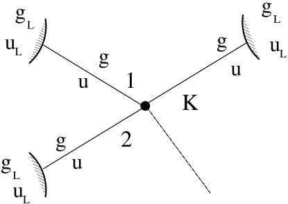
Figure 9: Sketch of a connected junction of $K$ wires with parameters $g,u$ connected to reservoirs with parameters $g_{L},u_{L}$.

C.2 Junction of strongly interacting quantum wires at $g_{c}=g_{s}=3$

As Eq. (97) applies independently of the specific form of the current operators, in order to generalize Eq. (109) to the strongly interacting case we discuss in Sec. III.2, one has just to compute the ${\cal D}_{(j,\sigma);(j^{\prime},\sigma^{\prime})}(x,t;x^{\prime},t^{\prime})$-terms in Eq. (96) using the current operators in the dual theory given in Eq. (49). As a result, one now obtains ${\cal D}_{(j,\sigma);(j^{\prime},\sigma^{\prime})}(x,x^{\prime};\omega)=\delta_{\sigma,\sigma^{\prime}}{\cal D}_{j,j^{\prime}}(x,x^{\prime};\omega)$, with

$${\cal D}_{j,j^{\prime}}(x,x^{\prime};\omega) = \frac{e^{2}}{2\pi}\>\int\>dE\>f(E)[f(-E-\omega)-f(-E+\omega)]$$ (110)

$$\times \Biggl{\{}2e^{i\frac{\omega}{u}(x-x^{\prime})}\delta_{j,j^{\prime}}+e^{i\frac{\omega}{u}(x+x^{\prime})}[|\tilde{S}_{j-1,j^{\prime}-1}|^{2}+|\tilde{S}_{j+1,j^{\prime}+1}|^{2}]$$

$$- e^{i\frac{\omega}{u}(x-x^{\prime})}[\delta_{j-1,j^{\prime}+1}+\delta_{j+1,j^{\prime}-1}]-e^{i\frac{\omega}{u}(x+x^{\prime})}[|\tilde{S}_{j-1,j^{\prime}+1}|^{2}+|\tilde{S}_{j+1,j^{\prime}-1}|^{2}]\Biggr{\}}\>\>\>\>.$$

Following the same steps as in Appendix C.1, from Eq. (110) one therefore readily derives the dc conductance tensor, which is given by

$$G_{(j,\sigma);(j^{\prime},\sigma^{\prime})}=\delta_{\sigma,\sigma^{\prime}}G_{j,j^{\prime}}\>\>\>\>,$$ (111)

with

$$G_{j,j^{\prime}} = \frac{e^{2}}{2\pi}\Biggl{\{}2\delta_{j,j^{\prime}}+|\tilde{S}_{j+1,j^{\prime}+1}|^{2}+|\tilde{S}_{j-1,j^{\prime}-1}|^{2}$$ (112)

$$- [\delta_{j+1,j^{\prime}-1}+\delta_{j-1,j^{\prime}+1}+|\tilde{S}_{j-1,j^{\prime}+1}|^{2}+|\tilde{S}_{j+1,j^{\prime}-1}|^{2}]\Biggr{\}}\>\>\>\>.$$

From Eq. (112) one therefore computes the conductance tensor at $g_{c}=g_{s}=3$. When either $g_{c}$, or $g_{s}$ (or both) are different from 3, using Eq. (112) one recovers the conductance tensor in the case in which $g_{c}$ and $g_{s}$ both asymptotically tend to 3 in the leads. The charge- and the spin-conductance tensors for the disconnected junction are obtained using Eq. (109) with $G_{{\rm in},c(s)}=\frac{2g_{c(s)}}{g_{c(s)}-1}\frac{e^{2}}{\pi}$.

References

- Landau (1957a) L. D. Landau, Sov. Phys. JETP 3, 920 (1957a).
- Landau (1957b) L. D. Landau, Sov. Phys. JETP 5, 101 (1957b).
- Landau (1958) L. D. Landau, Sov. Phys. JETP 8, 70 (1958).
- Abrikosov et al. (1963) A. A. Abrikosov, L. P. Gorkov, and I. E. Dzyaloshinski, Methods of Quantum field theory in statistical physics (Dover, New York, 1963).
- Fisher and Glazman (1997) M. P. A. Fisher and L. A. Glazman, in Mesoscopic Electron Transport, edited by G. S. L. Kouwenhoven and L. Sohn (NATO ASI Series E, Kluwer Ac. Publ., Dordrecht, 1997).
- Nozières (1964) P. Nozières, Theory of interacting Fermi systems (Addison-Wesley, Reading (MA), 1964).
- Sólyom (1979) J. Sólyom, Adv. Phys. 28, 201 (1979).
- Shankar (1994) R. Shankar, Rev. Mod. Phys. 66, 129 (1994).
- Polchinski (1993) J. Polchinski, in Proceedings of 1992 Theoretical Advanced Studies Institute in Elementary Particle Physics, edited by J. Harvey and J. Polchinski (World Scientific, Singapore, 1993).
- Furusaki and Nagaosa (1993) A. Furusaki and N. Nagaosa, Phys. Rev. B 47, 4631 (1993).
- Kane and Fisher (1992a) C. L. Kane and M. P. A. Fisher, Phys. Rev. Lett. 68, 1220 (1992a).
- Kane and Fisher (1992b) C. L. Kane and M. P. A. Fisher, Phys. Rev. B 46, 15233 (1992b).
- Matveev et al. (1993) K. A. Matveev, D. Yue, and L. I. Glazman, Phys. Rev. Lett. 71, 3351 (1993).
- Yue et al. (1994) D. Yue, L. I. Glazman, and K. A. Matveev, Phys. Rev. B 49, 1966 (1994).
- Nazarov and Glazman (2003) Y. V. Nazarov and L. I. Glazman, Phys. Rev. Lett. 91, 126804 (2003).
- Nayak et al. (1999) C. Nayak, M. P. A. Fisher, A. W. W. Ludwig, and H. H. Lin, Phys. Rev. B 59, 15694 (1999).
- Chen et al. (2002) S. Chen, B. Trauzettel, and R. Egger, Phys. Rev. Lett. 89, 226404 (2002).
- Lal et al. (2002) S. Lal, S. Rao, and D. Sen, Phys. Rev. B 66, 165327 (2002).
- Pham et al. (2003) K.-V. Pham, F. Piéchon, K.-I. Imura, and P. Lederer, Phys. Rev. B 68, 205110 (2003).
- Chamon et al. (2003) C. Chamon, M. Oshikawa, and I. Affleck, Phys. Rev. Lett. 91, 206403 (2003).
- Oshikawa et al. (2006) M. Oshikawa, C. Chamon, and I. Affleck, J. Stat. Mech. P02008 (2006).
- Rao and Sen (2004) S. Rao and D. Sen, Phys. Rev. B 70, 195115 (2004).
- Hou and Chamon (2008) C.-Y. Hou and C. Chamon, Phys. Rev. B 77, 155422 (2008).
- Jordan and Wigner (1928) P. Jordan and E. Wigner, Z. Phys. 47, 631 (1928).
- Eggert and Affleck (1992) S. Eggert and I. Affleck, Phys. Rev. B 46, 10866 (1992).
- Affleck (1998) I. Affleck, J. Phys. A 31, 2761 (1998).
- Crampe and Trombettoni (2013) N. Crampe and A. Trombettoni, Nucl. Phys. B 871, 526 (2013).
- Tsvelik (2013) A. M. Tsvelik, Phys. Rev. Lett 110, 147202 (2013).
- Reyes and Tsvelik (2005) S. A. Reyes and A. M. Tsvelik, Phys. Rev. Lett. 95, 186404 (2005).
- Giuliano et al. (2013) D. Giuliano, D. Rossini, P. Sodano, and A. Trombettoni, Phys. Rev. B 87, 035104 (2013).
- Glazman and Larkin (1997) L. I. Glazman and A. I. Larkin, Phys. Rev. Lett. 79, 3736 (1997).
- Giuliano and Sodano (2010) D. Giuliano and P. Sodano, Nucl. Phys. B 837, 153 (2010).
- Cirillo et al. (2011) A. Cirillo, M. Mancini, D. Giuliano, and P. Sodano, Nucl. Phys. B 852, 235 (2011).
- Béri and Cooper (2012) B. Béri and N. R. Cooper, Phys. Rev. Lett. 109, 156803 (2012).
- Galpin et al. (2014) M. R. Galpin, A. K. Mitchell, J. Temaismithi, D. E. Logan, B. Béri, and N. R. Cooper, Phys. Rev. B 89, 045143 (2014).
- Béri (2013) B. Béri, Phys. Rev. Lett. 110, 216803 (2013).
- Eriksson et al. (2014a) E. Eriksson, C. Mora, A. Zazunov, and R. Egger, Phys. Rev. Lett. 113, 076404 (2014a).
- Eriksson et al. (2014b) E. Eriksson, A. Nava, C. Mora, and R. Egger, Phys. Rev. B 90, 245417 (2014b).
- Tomonaga (1955) S. Tomonaga, Prog. Theor. Phys. 13, 467 (1955).
- Luttinger (1963) J. M. Luttinger, J. Math. Phys. 4, 1154 (1963).
- Haldane (1981a) F. D. M. Haldane, J. Phys. C: Solid State Phys. 14, 2585 (1981a).
- Haldane (1981b) F. D. M. Haldane, Phys. Rev. Lett. 47, 1840 (1981b).
- Das et al. (2006) S. Das, S. Rao, and D. Sen, Phys. Rev. B 74, 045322 (2006).
- Aristov (2011) D. N. Aristov, Phys. Rev. B 83, 115446 (2011).
- Fendley et al. (1995a) P. Fendley, A. W. W. Ludwig, and H. Saleur, Phys. Rev. Lett. 75, 2196 (1995a).
- Fendley et al. (1995b) P. Fendley, A. W. W. Ludwig, and H. Saleur, Phys. Rev. Lett. 74, 3005 (1995b).
- Fendley et al. (1995c) P. Fendley, A. W. W. Ludwig, and H. Saleur, Phys. Rev. B 52, 8934 (1995c).
- Rahmani et al. (2010) A. Rahmani, C.-Y. Hou, A. Feiguin, C. Chamon, and I. Affleck, Phys. Rev. Lett. 105, 226803 (2010).
- Rahmani et al. (2012) A. Rahmani, C.-Y. Hou, A. Feiguin, M. Oshikawa, C. Chamon, and I. Affleck, Phys. Rev. B 85, 045120 (2012).
- Sedlmayr et al. (2014) N. Sedlmayr, D. Morath, J. Sirker, S. Eggert, and I. Affleck, Phys. Rev. B 89, 045133 (2014).
- Feiguin and White (2005) A. E. Feiguin and S. R. White, Phys. Rev. B 72, 220401(R) (2005).
- Karrasch et al. (2012) C. Karrasch, J. H. Bardarson, and J. E. Moore, Phys. Rev. Lett. 108, 227206 (2012).
- Meden et al. (2003) V. Meden, S. Andergassen, W. Metzner, U. Schollwöck, and K. Schönhammer, Europhys. Lett. 64, 769 (2003).
- Andergassen et al. (2004) S. Andergassen, T. Enss, V. Meden, , W. Metzner, U. Schollwöck, and K. Schönhammer, Phys. Rev. B 70, 075102 (2004).
- Meden et al. (2005) V. Meden, T. Enss, S. Andergassen, W. Metzner, and K. Schönhammer, Phys. Rev. B 71, 041302(R) (2005).
- Enss et al. (2005) T. Enss, V. Meden, S. Andergassen, X. Barnabe-Theriault, W. Metzner, and K. Schönhammer, Phys. Rev. B 71, 155401 (2005).
- Andergassen et al. (2006) S. Andergassen, T. Enss, V. Meden, W. Metzner, U. Schollwöck, and K. Schönhammer, Phys. Rev. B 73, 045125 (2006).
- Barnabe-Theriault et al. (2005a) X. Barnabe-Theriault, A. Sedeki, V. Meden, and K. Schönhammer, Phys. Rev. Lett. 94, 136405 (2005a).
- Meden et al. (2006) V. Meden, S. Andergassen, T. Enss, H. Schöller, and K. Schönhammer, New Journal of Physics 10, 045012 (2006).
- Barnabe-Theriault et al. (2005b) X. Barnabe-Theriault, A. Sedeki, V. Meden, and K. Schönhammer, Phys. Rev. B 71, 205327 (2005b).
- Janzen et al. (2006) K. Janzen, V. Meden, and K. Schönhammer, Phys. Rev. B 74, 085301 (2006).
- Jakobs et al. (2007) S. G. Jakobs, V. Meden, H. Schöller, and T. Enss, Phys. Rev. B 75, 035126 (2007).
- Titov et al. (2006) M. Titov, M. Müller, and W. Belzig, Phys. Rev. Lett. 97, 237006 (2006).
- Schulz (1980) H. J. Schulz, Phys. Rev. B 22, 5274 (1980).
- Aristov and Wölfle (2012) D. N. Aristov and P. Wölfle, Phys. Rev. B 86, 035137 (2012).
- Aristov and Wölfle (2013) D. N. Aristov and P. Wölfle, Phys. Rev. B 88, 075131 (2013).
- Aristov and Wölfle (2011) D. N. Aristov and P. Wölfle, Phys. Rev. B 84, 155426 (2011).
- von Delft and Schoeller (1998) J. von Delft and H. Schoeller, Annalen Phys. 7, 225 (1998).
- Hou et al. (2012) C.-Y. Hou, A. Rahmani, A. E. Feiguin, and C. Chamon, Phys. Rev. B 86, 075451 (2012).
- Das et al. (2008) S. Das, S. Rao, and A. Saha, Phys. Rev. B 77, 155418 (2008).
- Affleck and Giuliano (2012) I. Affleck and D. Giuliano, J. Stat. Mech. P06011 (2012).
- Fidkowski et al. (2012) L. Fidkowski, J. Alicea, N. H. Lindner, R. M. Lutchyn, and M. P. A. Fisher, Phys. Rev. B 85, 245121 (2012).
- Giuliano and Affleck (2013) D. Giuliano and I. Affleck, J. Stat. Mech. P02034 (2013).
- Giuliano and Affleck (2014) D. Giuliano and I. Affleck, Phys. Rev. B 90, 045133 (2014).
- Affleck and Giuliano (2014) I. Affleck and D. Giuliano, J. Stat. Phys. , Special Issue in Memory of K. G. Wilson 157, 666 (2014).
- Shultz et al. (1997) H. J. Shultz, G. Cuniberti, and P. Pieri, in Field Theory for Low-Dimensional Condensed Matter Systems, edited by V. T. G.Morandi, P. Sodano and A. Tagliacozzo (Springer-Verlag, 1997).
- Gogolin et al. (2004) A. O. Gogolin, A. A. Nersesyan, and A. M. Tsvelik, Bosonization and Strongly Correlated Systems (Cambridge University Press, 2004).
- Sugiyama (1980) T. Sugiyama, Prog. Theor. Phys. 64, 406 (1980).
- Maslov and Stone (1995) D. L. Maslov and M. Stone, Phys. Rev. B 52, R5539 (1995).