Search for exotic short-range interactions using paramagnetic insulators

Abstract

We describe a proposed experimental search for exotic spin-coupled interactions using a solid-state paramagnetic insulator. The experiment is sensitive to the net magnetization induced by the exotic interaction between the unpaired insulator electrons with a dense, non-magnetic mass in close proximity. An existing experiment has been used to set limits on the electric dipole moment of the electron by probing the magnetization induced in a cryogenic gadolinium gallium garnet sample on application of a strong electric field. With suitable additions, including a movable source mass, this experiment can be used to explore “monopole-dipole” forces on polarized electrons with unique or unprecedented sensitivity. The solid-state, non-magnetic construction, combined with the low-noise conditions and extremely sensitive magnetometry available at cryogenic temperatures could lead to a sensitivity over ten orders of magnitude greater than exiting limits in the range below 1 mm.

Introduction.— Experimental searches for macroscopic forces beyond gravity and electromagnetism have received a great deal of attention in the past two decades. Present limits allow for unobserved forces several million times stronger than gravity acting over distances of a few microns. Predictions of unobserved forces in this range have arisen in several contexts, including attempts to describe gravity and the other fundamental interactions in the same theoretical framework. For comprehensive reviews, see Adelberger et al. (2009); Antoniadis et al. (2011); Jaeckel and Ringwald (2010). The sub-millimeter range has been the subject of active theoretical investigation, notably on account of the prediction of “large” extra dimensions at this scale which could explain the hierarchy problem Arkani-Hamed et al. (1998). The fact that the dark energy density, of order (1 meV)⁴, corresponds to a length scale of about 100 $\mu$m also encourages searches for unobserved phenomena at this scale. Many theories beyond the Standard Model possess extended symmetries that, when broken at high energy scales, give rise to light bosons with very weak couplings to matter. Examples include moduli Dimopoulos and Geraci (2003), dilatons Kaplan and Wise (2000), and the axion–a light pseudoscalar motivated by the strong CP problem of QCD Peccei and Quinn (1977). These particles can generate weak, relatively long-range interactions between samples of ordinary matter, including interactions that couple to spin. In a seminal paper Moody and Wilczek (1984), Moody and Wilczek derived three possible interactions for the axion, and proposed searches sensitive to the $T$-violating “monopole-dipole” interaction between polarized and unpolarized test masses.

We propose an experimental search for exotic spin-coupled interactions using a solid-state paramagnetic insulator as a detector. The candidate material is gadolinium gallium garnet (Gd₃Ga₅O₁₂, or GGG), which has been used as a detector in an experimental search for the electric dipole moment (EDM) of the electron Kim et al. . (See Sushkov et al. (2009); Eckel et al. (2012) for realizations of other EDM materials.) In that experiment, the signal is an induced sample magnetization on application of a strong external electric field; in our proposal the magnetization is induced by an exotic monopole-dipole interaction with a dense, non-magnetic mass brought into close proximity. An exotic field coupling to the electron spins of an atom or an ion with spin $S=\sqrt{s(s+1)}$ in the solid sample leads to a net spin excess in the sample. At the location of a particular ion in the sample, the spin excess ratio is given by Kittel and Kroemer (1980); Abragam (1978)

$$R=\frac{\displaystyle\sum_{m_{s}=-s}^{s}m_{s}e^{\frac{m_{s}u/\sqrt{s(s+1)}}{kT}}}{\displaystyle\sum_{m_{s}=-s}^{s}e^{\frac{m_{s}u/\sqrt{s(s+1)}}{kT}}},$$ (1)

where $m_{s}$ is the magnetic quantum number, $u$ is the local exotic field energy per ion, $T$ is the sample temperature and $k$ is Boltzmann’s constant. In our proposal, the energy shift predicted from the exotic coupling at the current experimental limits is much smaller than the thermal energy. However, the cumulative effect from the large number of electrons in a macroscopic, solid-state sample leads to a net spin alignment on the order of $10^{9}$ Bohr magnetons cm^-3. The resulting sample magnetization can be probed with great sensitivity using sensors based on superconducting quantum interference device (SQUID) technology.

The idea of using solid-state materials with bound but unpaired electron spins to probe exotic fields was first proposed by Shapiro in 1968 Shapiro (1968) in the context of EDM searches. Recently, other fundamental applications of these materials have been proposed, including tests of Lorentz and $CPT$ invariance Bluhm and Kostelecky (2000). Experiments using EDM techniques, but on a different class of solid-state materials, have been proposed to search for cosmic axions Budker et al. (2014). Many experiments have been performed to search for spin-dependent macroscopic interactions using other methods. Examples include NMR-type experiments sensitive to precession frequency shifts in various materials, including the paramagnetic salt TbF₃ Ni et al. (1999), Hg and Cs comagnetometers Youdin et al. (1996), polarized ¹²⁹Xe and ¹³¹Xe gas Bulatowicz et al. (2013), and polarized ³He gas Vasilakis et al. (2009); Chu et al. (2013); Tullney et al. (2013), in the presence of polarized and unpolarized masses. Other experiments search for effects in torsion pendulums Ritter et al. (1993); Hammond et al. (2007); Heckel et al. (2008); Hoedl et al. (2011), neutron bound states in the Earth’s gravitational field Baessler et al. (2007); Jenke et al. (2014), and longitudinal and transverse spin relaxation of polarized neutrons and ³He Serebrov (2009); Pokotilovski (2010); Petukhov et al. (2010); Fu et al. (2011); Petukhov et al. (2011). An overview can be found in Antoniadis et al. (2011). Other parameters being equal, the proposed solid-state technique affords an enhancement factor on the order of the Avogadro number relative to experiments in dilute vapor systems, though the latter are primarily sensitive to polarized nucleon couplings. With suitable control of systematic effects, the ultimate sensitivity is more than 10 orders of magnitude greater than current laboratory limits in the range below 1 cm, and the technique is sensitive to exotic interactions of electrons presently unconstrained by either laboratory experiments or astrophysical observations.

A study by Dobrescu and Mocioiu Dobrescu and Mocioiu (2006) of the possible interactions between non-relativistic fermions assuming only rotational invariance revealed 15 forms for the potential involving the fermion spins. Nine of these are spin-spin interactions, which would necessitate spin-polarized test masses with low intrinsic magnetism Ritter et al. (1990); Leslie et al. (2014); here we concentrate on monopole-dipole interactions between polarized and unpolarized objects. In the zero-momentum transfer limit, the possible interactions between a polarized electron and an unpolarized atom or molecule of atomic number $Z$ and mass $A$ are (in SI units, and adopting the numbering scheme in Dobrescu and Mocioiu (2006)):

$$V_{4+5} = \left(g_{A}^{e}\right)^{2}\frac{\hbar^{2}}{16\pi m_{e}c}Z\left[\hat{\sigma}\cdot(\vec{v}\times\hat{r})\right]\left(\frac{1}{\lambda r}+\frac{1}{r^{2}}\right)e^{-r/\lambda},$$

$$V_{9+10} = g_{P}^{e}g_{S}^{N}\frac{\hbar^{2}}{8\pi m_{e}}A(\hat{\sigma}\cdot\hat{r})\left(\frac{1}{\lambda r}+\frac{1}{r^{2}}\right)e^{-r/\lambda},$$

$$V_{12+13} = g_{A}^{e}g_{V}^{N}\frac{\hbar}{4\pi}A(\hat{\sigma}\cdot\vec{v})\left(\frac{1}{r}\right)e^{-r/\lambda}.$$ (2)

Here $\vec{S}=\hbar\hat{\sigma}/2$ is the electron spin, $\hbar$ is Planck’s constant, $\hat{r}=\vec{r}/r$ is a unit vector along the direction between the electron and atom, $\vec{v}$ is their relative velocity, $c$ is the speed of light in vacuum, $m_{e}$ is the electron mass, and $\lambda$ is the interaction range. The factors $g_{P}^{e}$ and $g_{A}^{e}$ are the electron pseudoscalar and axial vector coupling constants, and $g_{S}^{N}$ and $g_{V}^{N}$ are the nucleon scalar and vector couplings. The couplings in Eq. 2 are not the most general Dobrescu and Mocioiu (2006); we have included those for which the proposed experiment will likely have the greatest discovery potential. We note that $V_{9+10}$ can also proceed via a spin-1 interaction, in which case the coupling is $g_{A}^{e}g_{V}^{N}$. $V_{4+5}$ can also proceed via a spin-0 interaction, in which case the coupling is $g_{S}^{e}g_{S}^{N}$ (and the expression for $V_{4+5}$ above is scaled by $A/Z$).

The experiment is illustrated schematically in Fig. 1. It is based directly on the apparatus used in Kim et al. ; many parameters have been retained for the purposes of designing a practical device. A solid paramagnetic insulating sample or “detector” mass, in the form of a block or disk, is mounted in the sample space of a large dilution refrigerator. A dense, unpolarized, non-magnetic insulator of similar size and shape is brought into close proximity and serves as “source” mass. The source–detector gap can be modulated (e.g., via translation or rotation stages) from 0–1 cm with the resolution of a few microns. The non-magnetic design eliminates the need for shielding between the test masses. At closest approach, the source is essentially in contact with the detector, permitting force searches with potentially unprecedented sensitivity in the range below 1 mm. The detector magnetization induced by the exotic interaction with the source is sensed by a pickup coil surrounding the detector. The coil is coupled to a sensitive SQUID magnetometer.

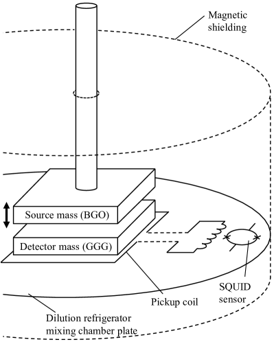
Figure 1: Schematic of proposed experiment. A dense, non-magnetic planar source mass is modulated vertically above a paramagnetic detector mass, inducing a magnetization read out with the pickup coil and SQUID sensor. The detector is kept at temperatures near 1 K.

For the detector material we assume GGG, as in Kim et al. . The use of GGG was first proposed in Lamoreaux (2002) and realized in Liu and Lamoreaux (2004). The material is chosen to maximize the induced spin density. GGG contains a high density of Gd³⁺ ions ($\approx 10^{22}$/cm³), each of which has seven electrons in the 4f shell: the shell is thus half-filled and all electrons are unpaired Geller (1978). This property leads to a relatively strong magnetic response to external fields. For the source mass we assume bismuth germanate (Bi₄Ge₃O₁₂, or BGO), a high density, non-magnetic insulator Tullney et al. (2013).

Experimental Sensitivity.— An approximate sensitivity and figure-of-merit can be derived using a simplified geometry; we examine the case of the $V_{9+10}$ interaction, which is the most widely studied. The interaction energy between an unpolarized, flat–plate source mass parallel to a flat–plate paramagnetic detector mass is given by:

$$U_{9+10} = g_{P}^{e}g_{S}^{N}\frac{\hbar^{2}}{4m_{e}}A_{m}n_{m}n_{d}S_{d}a_{d}$$ (3)

$$\times\lambda^{2}e^{-z(t)/\lambda}(1-e^{-t_{m}/\lambda})(1-e^{-t_{d}/\lambda}),$$

where $n_{m}$ is the number density of molecules in the source mass and $A_{m}$ is their mass number, $n_{d}$ is the number density of polarized ions in the detector mass and $S_{d}$ is the ion spin, $a_{d}$ is the detector area, $z(t)$ is the source–detector gap, and $t_{m}$ and $t_{d}$ are the source and detector thicknesses. This expression is exact for the case of a source of infinite area, in which case the detector spins align toward the source, in the direction normal to the detector plane. For the practical case of a finite source (considered in detail below), there are edge corrections (which are the dominant effect in the $V_{4+5}$ case; see Eq. 2). The proposed experiment is sensitive to changes in the induced field as the source mass is modulated, which we assume to occur at some fixed frequency $\omega$ significantly above the 1/f noise corner of the SQUID. The noise corner was about 0.1 Hz for the SQUID in Kim et al. ; we assume $\omega/2\pi=1$ Hz. From Fourier analysis, the amplitude of the energy change per detector ion at $\omega$ is

$$\tilde{u}_{9+10}=A_{m}g_{P}^{e}g_{S}^{N}\frac{\hbar^{2}}{2m_{e}}n_{m}S_{d}\lambda I_{1}(z_{0}/\lambda)e^{-\bar{z}/\lambda}(1-e^{-t_{m}/\lambda}),$$ (4)

where $\tilde{u}_{9+10}=\tilde{U}_{9+10}/N_{d}$ and $N_{d}=n_{d}a_{d}t_{d}$ is the number of detector spins. In Eq. 4 we have taken the limit $\lambda\gg t_{d}$, so that $\tilde{u}_{9+10}$ is a good approximation at the location of any particular ion in the detector mass (or, equivalently, in a layer of thickness $\approx\lambda$ at the top surface of a thicker detector). Here, $I_{1}(z_{0}/\lambda)$ is the modified Bessel function, and we have used $z(t)=\bar{z}+z_{0}\sin{\omega t}$ where $\bar{z}=(z_{\mbox{\scriptsize max}}+z_{\mbox{\scriptsize min}})/2$ is the average source–detector gap and $z_{0}=(z_{\mbox{\scriptsize max}}-z_{\mbox{\scriptsize min}})/2$ is the amplitude of the source mass motion.

In the limit $\tilde{u}_{9+10}\ll kT$, the spin excess ratio (Eq. 1) can be approximated as $R=\tilde{u}_{9+10}/(3kT)$, whereby the total spin excess in the layer is $S_{d}N_{d}\tilde{u}_{9+10}/(3kT)$. The layer magnetization normal to the plane is

$$M=\frac{g\mu_{B}S_{d}n_{d}\tilde{u}_{9+10}}{3kT},$$ (5)

where $g=2$ for electrons and $\mu_{B}$ is the Bohr magneton. As in Kim et al. , we assume the plane of the pickup coil to be situated just below the bottom surface of the detector mass (Fig. 1). The field of the magnetized slab of thickness $\lambda$ just below the bottom is slowly-varying across the surface, with a minimum at the center of $B_{z}\approx\mu_{0}M\lambda/\sqrt{a_{d}}$. Assuming a coil area of $a_{d}$, a conservative estimate of the induced flux through the coil is thus $\Phi_{i}\approx\mu_{0}fM\lambda\sqrt{a_{d}}$, where we include a suppression factor $f$ for sub-optimal coupling between the detector and coil.

In an experiment using a practical SQUID sensor, the pickup coil connects to a built-in input coil on the sensor. The changing flux from the detector induces a current, which flows into the input coil and produces a flux that couples inductively to the SQUID loop and is transduced to a voltage. The relationship between the magnetic flux $\Phi_{i}$ picked up from the detector mass and the induced flux $\Phi_{sq}$ in the SQUID loop is Kim et al.

$$\Phi_{sq}=\frac{M}{L_{p}+L_{i}}\Phi_{i}=\beta\Phi_{i},$$ (6)

where $L_{p}$ and $L_{i}$ are the inductances of the pickup and input coils, respectively, and $M$ is the mutual inductance between the input coil and SQUID. The factor $\beta$ is the coupling efficiency which quantifies the flux reduction when $\Phi_{i}$ is delivered to the SQUID sensor.

The sensitivity of the experiment is based on the expectation that essentially all backgrounds can be suppressed below the intrinsic noise of the SQUID sensor. In an experiment limited by this noise ($\phi_{n}$, expressed in terms of magnetic flux per root bandwidth), the signal-to-noise ratio is given by:

$$SNR=\frac{\Phi_{sq}\sqrt{\tau}}{\phi_{n}},$$ (7)

where $\tau$ is the integration time. The sensitivity is calculated by setting $SNR=1$ and solving for $g_{P}g_{S}$. Combining Eqs. 3 through 7, the result is:

$$g_{P}^{e}g_{S}^{N}=\frac{4\mu_{B}m_{e}\mbox{u}}{\hbar^{2}}\frac{1}{\rho_{m}}\frac{1}{\lambda^{2}\epsilon}\frac{1}{\beta f}\frac{\phi_{n}}{\sqrt{\tau}}\frac{1}{\sqrt{a_{d}}}\left(\frac{1}{\chi_{d}}+D\right).$$ (8)

Here we have used $n_{m}=\rho_{m}/(\mbox{u}A_{m})$, where $\rho_{m}$ is the mass density of the source and u is the atomic mass unit. The factor $\chi_{d}$ is the effective susceptibility of the detector mass:

$$\chi_{d}=\frac{4\mu_{0}\mu_{B}^{2}n_{d}S_{d}^{2}}{3kT},$$ (9)

and we have used $\chi_{d}\rightarrow\chi_{d}/(1+D\chi_{d})$ in Eq. 8, where $D$ is the demagnetization factor. The efficiency $\epsilon\equiv I_{1}(z_{0}/\lambda)e^{-\bar{z}/\lambda}(1-e^{-t_{m}/\lambda})$ in Eq. 8 is of order unity for an optimized vertical geometry.

A plot of $g_{P}^{e}g_{S}^{N}$ vs $\lambda$ from Eq. 8 is shown in Fig. 3, using the parameters in Tables 1 and 2. We assume the source and detector can be brought into contact but also that these elements can only be made flat to within a few microns, thus the minimum gap is set to 10 $\mu$m. For each value of $\lambda$, the maximum separation $z_{\mbox{\scriptsize max}}$ is chosen to maximize $\epsilon$, which occurs around $z_{\mbox{\scriptsize max}}=3\lambda$. The efficiency is maximized for $t_{m}\rightarrow\infty$, however, since very little is gained for $t_{m}>\lambda$, we set $t_{m}=1$ cm, about twice the maximum range of interest. A suppression factor of $f=0.4$ has been used, in accordance with Kim et al. . For a rectangular prism of square cross-section $a_{d}$ magnetized parallel to the thickness (here $\approx\lambda$), we have used the approximation $D\approx\sqrt{a_{d}}/(\sqrt{a_{d}}+2\lambda)$ Sato and Ishii (1989).

From Eq. 8, an approximate figure-of-merit for the experiment is:

$$FOM=\rho_{m}\epsilon\beta f\frac{\sqrt{\tau}}{\phi_{n}}\sqrt{a_{d}}\frac{\chi_{d}}{1+D\chi_{d}},$$ (10)

illustrating the importance of high $\rho_{m}$, and $\bar{z}\approx z_{0}\approx\lambda$ (through $\epsilon$). Over the range of interest, $D$ varies between 0.75 and 1. Thus it is important that $\chi_{d}$ be at least of order unity, but larger values will yield little improvement for the chosen detector geometry. We note Eq. 9 suggests $\chi_{d}$ could be improved by several orders of magnitude by operation at the sub-Kelvin temperatures available in dilution refrigerators. However, as discussed in Kim et al. , the susceptibility of practical paramagnetic insulators is well described by a Curie-Weiss relation of the form $\chi=C/(T-T_{CW})$, where $|T_{CW}|$ represents an effective minimum temperature assuming the operating temperature is lower. Following Kim et al. , we use $T_{CW}=-2.1$ K. We assume an operating temperature of 1.0 K, the lowest temperature at which the susceptibility obeys the Curie-Weiss law Schiffer et al. (1995). This leads to an effective temperature of $T=3.1$ K in Eq. 9 and an estimate of $\chi_{d}=0.53$ (Table 1), slightly below the value measured in Schiffer et al. (1995) for single-crystal GGG. Optimization of other terms in Eq. 10 is discussed below.

Table 1: Parameters used in the sensitivity computation.

Parameter	Value
effective area of pickup coil, $a_{c}$	12.75 cm2
source mass density (BGO), $\rho_{m}$	7.13 g/cm3
detector spin density, $n_{d}$	$10^{22}/$cm3
detector spin/Gd ion, $s$	$7/2$
detector susceptibility, $\chi_{d}$	$0.53$ (SI)
coupling efficiency, $\beta$	$7.8\times 10^{-3}$
sensor intrinsic noise, $\phi_{n}$	$3\mu\Phi_{0}/\sqrt{\mbox{Hz}}$
integration time, $\tau$	$10^{6}$ s

Table 2: Dimensions of the detector and source masses used in the sensitivity calculations.

Parameter	Value
detector width, $x_{d}$	3.00 cm
detector length, $y_{d}$	3.00 cm
detector thickness, $z_{d}$	0.76 cm
source mass width, $x_{m}$	3.00 cm
source mass length, $y_{m}$	3.00 cm
source mass thickness, $z_{m}$	1.00 cm
minimum gap, $z_{min}$	10 $\mu$m

For more accurate estimates of the sensitivity of a practical experiment to each potential in Eq. 2, we perform numerical calculations, in which all approximations used above are relaxed. The theoretical interactions from each potential due to a finite-sized source are computed at representative points in a hypothetical, practically-shaped detector and used to generate a spin excess profile as a function of the spatial coordinates. This profile is then used in a finite element (FEA) model to create a map of the induced flux $\Phi_{i}$ in the region of the detector and pickup coil.

The detector is broken up into subvolumes and the potentials calculated by Monte Carlo integration between the center point of each subvolume and the complete volume of the source mass. The detector and source dimensions (very similar to those used for the sample in Kim et al. ) are given in Table 2. The induced spin orientation at each subvolume location is obtained by repeating the calculation for many possible orientations and taking the maximum. The integration models the modulation of the source mass (assumed sinusoidal) and records the results at several values of the separation (that is, the source phase) over a complete period. A minimum source-sample gap of 10 $\mu$m is used as in the analytical estimate. The maxima are then converted to magnetization vectors for each subvolume and phase using Eq. 1 and the parameters in Table 1. Fig. 2 shows a detector magnetization map for the case of the $V_{9+10}$ interaction with $\lambda=5$ mm at a particular source phase.

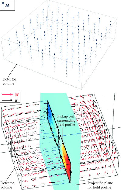
Figure 2: (Color online)Top: map of detector mass magnetization induced by source in $V_{9+10}$ interaction. Vectors represent magnetization (each an average of one of 343 subvolumes). Bottom: magnetization (light arrows) and magnetic field (black arrows) induced by source in $V_{4+5}$ interaction. Flux is calculated through cross section; dotted line shows placement of pickup coil for $V_{4+5}$ experiment. In both cases $\lambda=5$ mm, and source (not shown) is slab of identical area centered above detector at instantaneous separation of 3 mm.

Magnetization maps are then entered into an electromagnetic FEA model of the sample generated with the COMSOL software package com . The model interpolates between the points of the input data to generate a complete magnetization profile within the detector volume and a complete field profile in the interior and exterior. An example field profile is shown in Fig. 2.

From these profiles, the flux through the area of the pickup coils in the proposed experiment is calculated. Following Kim et al. , we assume a planar gradiometer design for the pickup coil for the $V_{9+10}$ and $V_{12+13}$ interactions, to reduce common-mode backgrounds; the coil area in Table 1 matches that in Kim et al. . For the $V_{4+5}$ interaction, the coil takes the planar “figure-8” form shown in Fig. 2 for similar common-mode rejection, either sandwiched between two halves of a split detector or wound through a small vertical hole in the center. For a particular interaction in Eq. 2 at a given range $\lambda$, the experimental signal is calculated by taking the Fourier transform of the flux though the gradiometer coil as a function of the source phase, and scaling the result by the reduction factor in Eq. 6. For each value of $\lambda$ investigated, the source mass amplitude is optimized for maximum signal, resulting in amplitudes of order $\lambda$. Finally, the $SNR$ is obtained by dividing this result by the sensor intrinsic noise (Table 1). The coupling constants in Eq. 2 are then adjusted so that $SNR=1$, resulting in the sensitivity curves in Fig. 3.

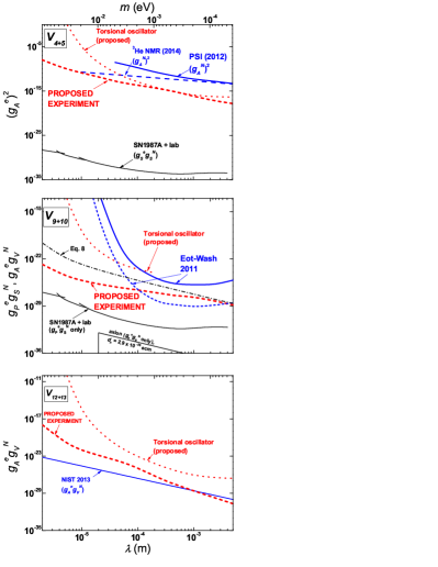
Figure 3: (Color online) Projected sensitivity of proposed experiment to $V_{4+5}$, $V_{9+10}$, and $V_{12+13}$ interactions, in which couplings are plotted versus range $\lambda$ (lower axes) or mass of unobserved boson (upper axes). Bold solid (dashed) curves are current (preliminary) limits, fine solid curves are indirect limits, dotted curves are proposals, dot-dash curve is Eq. 8. See text for explanations.

The velocity-dependent interactions $V_{4+5}$ and $V_{12+13}$ are unconstrained for the case of polarized electrons. (We note that, if $V_{4+5}$ is interpreted exclusively as an axial-vector interaction, the coupling $(g_{A}^{e})^{2}$ is tightly constrained by electron spin-spin experiments Ritter et al. (1990); Heckel et al. (2013); Kotler et al. .) For rough comparison, the bold solid line in the $V_{4+5}$ plot is the limit on the corresponding coupling for polarized nucleons from the experiment at the Paul Scherrer Institute Piegsa and Pignol (2012); the long-dashed line is the preliminary limit on the nucleon coupling from Zhang et al. . Similarly, the bold solid line in the $V_{12+13}$ plot is the limit on the corresponding polarized nucleon coupling derived from the neutron spin rotation experiment at NIST Yan and Snow (2013).

The best limit on the $V_{9+10}$ interaction for electrons derives from the axionlike particle torsion pendulum in the Eot-Wash group Hoedl et al. (2011). This limit is indicated by the bold line in the $V_{9+10}$ plot; the dotted line below it is the projected thermal limit. The sensitivity of the proposed experiment ranges from two to over ten orders of magnitude greater in the range of interest. It is in good agreement with the analytical estimate from Eq. 8 at large $\lambda$ where $\lambda\approx t_{d}$, suggesting that $t_{d}$ better estimates the depth to which the detector is significantly magnetized.

The fine solid lines in the $V_{4+5}$ and $V_{9+10}$ plots are the limits obtained from combining the constraints on $g_{S}^{e}$ or $g_{P}^{e}$ from the inferred cooling rate of SN1987A with the constraints on $g_{S}^{N}$ from spin-independent short-range fifth force experiments Raffelt (2012). These apply to spin-0 interactions and are thus for illustrative purposes only in the case of $V_{4+5}$. The $V_{9+10}$ limits are still more stringent than the projections for the direct search proposed, though the latter are more general and free from uncertainties related to dense nuclear matter effects in stars.

The $V_{9+10}$ plot also shows the limit inferred from the constraint on the electric dipole of the neutron ($d_{n}$) Baker et al. (2006), which sets bounds on $g_{S}^{N}$ via the QCD $\theta$-term and thus is restricted to case of the (spin-0) axion. For generic light scalars unrelated to the strong CP problem, the limits from direct searches are more stringent than those inferred from EDM bounds over the range of interest Mantry et al. (2014). Thus, correlating observations in EDM and macroscopic experiments could help distinguish axions from more generic light scalars.

The light dotted lines in each plot are the projected sensitivity of the proposed experiment in Leslie et al. (2014). That proposal is sensitive to polarized electron coupling and competes directly, but our projections are stronger by about 1-10 orders of magnitude for all interactions. A proposal for a direct experiment sensitive to the axion region in the $V_{9+10}$ plot is described in Arvanitaki and Geraci (2014), though that experiment is sensitive to polarized nucleon coupling.

Backgrounds.— The analysis above assumes the sensitivity of the experiment to be limited by the intrinsic noise of the SQUID sensor. Both GGG and BGO are good electrical insulators so Johnson noise levels are expected to be very low, however, magnetic noise due to dissipation in the test masses is another possible statistical background. The spectral density of magnetization noise in the detector mass is given by Eckel et al. (2009); Sushkov et al. (2009):

$$M_{\omega}\approx\frac{1}{\mu_{0}}\sqrt{\frac{kT\mu^{\prime\prime}}{V\omega}},$$ (11)

where $V$ is the volume and $\mu^{\prime\prime}$ is the imaginary part of the complex permeability. While data on $\mu^{\prime\prime}$ for the proposed GGG detector material are not available, it is expected to be too small (and even smaller in BGO, which has much lower susceptibility) for this noise to be observable. It was not observed, for example, in the experiment in Kim et al. , results from which were consistent with SQUID noise after 5 days of integration time.

Systematic effects are a greater concern. For example, the source can acquire a magnetization $M_{m}=\chi_{m}B_{0}/\mu_{0}$ via the interaction of its susceptibility $\chi_{m}$ with a stray field $B_{0}$. The changing flux through the pickup coil as the source oscillates above it can mimic a signal. BGO is diamagnetic with $\chi_{m}=-1.9\times 10^{-5}$ at room temperature Yamamoto et al. (2003), however there is evidence that it is weakly paramagnetic in low fields. Low-temperature data on $\chi_{m}$ of pure BGO are not available, but the related compound $\alpha$-Bi₂O₃ exhibits $\chi_{m}\approx 1.8\times 10^{-6}$ at 4 K in low fields Kravchenko et al. (2006). We estimate the flux as $d\phi\approx(\partial B/\partial z)z_{0}a_{d}$, where $\partial B/\partial z$ is the gradient above the center of a magnetized disk of area $a_{d}$ a distance $z_{d}$ above the coil (Table 2), and $z_{0}$ is the largest source amplitude. Requiring $d\phi<\phi_{n}/\sqrt{\tau}$ leads to an upper limit on the allowed stray field of $B_{0}\approx 10^{-12}$ T. Assuming typical stray laboratory fields on the order of $10^{-4}$ T, the required shielding factor is $10^{8}$. This is quite modest compared to the experiment in Kim et al. , which used two layers of superconducting lead foils and three layers of mu-metal sheets wound on frames to attain a measured shielding factor of $5\times 10^{11}$ (which we assume here).

Vibrations are potentially more troublesome. Motion of the detector-pickup coil assembly in phase with the source drive could induce a signal in the presence of a stray gradient $\partial B_{0}/\partial z$, given by $d\phi\approx(\partial B_{0}/\partial z)\delta z_{d}a_{d}$, where $\delta z_{d}$ is the assembly vibration amplitude. This signal is common-mode; the common-mode rejection ratio of the pickup coil used in Kim et al. was about $2\times 10^{2}$. Dividing the estimate for $d\phi$ by this factor and again demanding $d\phi<\phi_{n}/\sqrt{\tau}$ leads to a requirement on the stray gradient of $\partial B_{0}/\partial z<10^{-12}$ T/m per micron of assembly vibration. Assuming typical lab gradients of order $10^{-3}$ T/m, this is within the shielding factor for vibrations less than about 100 $\mu$m. If the vibrations cause the assembly to tilt in a stray field of $10^{-12}$ T, the resulting flux signal estimate falls below the noise as long as the vibrations are less than about 30 $\mu$m. These effects can be studied by examining signals in the absence of a detector mass. The simple translating source mass assumed can be replaced by a rotor with several segments of alternating density that pass over the detector at a multiple of the rotary drive frequency Chen et al. ; Arvanitaki and Geraci (2014), thus decoupling the drive frequency from the actual source modulation.

Conclusions.— We have performed detailed calculations of the projected sensitivity of an exotic interaction search with a paramagnetic insulating detector at cryogenic temperatures. The proposed technique affords the possibility to probe the interaction between macroscopic test masses in near contact in a low-noise environment. Our results indicate either unique sensitivity to electron “monopole–dipole” interactions in the range below 1 mm, or improvements of more than ten orders of magnitude over existing experiments. The statistical limits in Fig. 3 represent the ultimate practical sensitivity of the experiment and are ambitious long–term goals. Results with reduced but competitive sensitivity, likely limited by systematics, are expected much sooner. The proposed technique is based largely on a proven design. Our primary purpose has been to show the potential sensitivity of that design, especially with the parameters of the existing detection scheme. Technical challenges associated with source mass translation in the cryostat and the related systematic backgrounds will certainly have to be addressed. Possible improvements include better SQUID coupling efficiency ($\beta$ in Eq. 10), though this is a subtle optimization problem Sushkov et al. (2009). Increasing the detector area $a_{d}$ (Eq. 10 scales as $\sqrt{a_{d}}$, given the near saturation of the demagnetization factor) is another possibility, though problems of test mass metrology and changes to SQUID coupling efficiency will warrant careful study.

Acknowledgments.— The authors thank H. Gao, E. Smith, A. Holley, and W. M. Snow for useful discussions. This work is supported by National Science Foundation Grants PHY-1207656, PHY-1306942, Duke University, Los Alamos National Laboratory, and the Indiana University Center for Spacetime Symmetries (IUCSS).

References

- Adelberger et al. (2009) E. Adelberger, J. Gundlach, B. Heckel, S. Hoedl, and S. Schlamminger, Prog. Part. Nucl. Phys. 62, 102 (2009).
- Antoniadis et al. (2011) I. Antoniadis, S. Baessler, M. Buchner, V. Fedorov, S. Hoedl, et al., Comptes Rendus Physique 12, 755 (2011).
- Jaeckel and Ringwald (2010) J. Jaeckel and A. Ringwald, Ann. Rev. Nucl. Part. Sci. 60, 405 (2010), arXiv:1002.0329 [hep-ph] .
- Arkani-Hamed et al. (1998) N. Arkani-Hamed, S. Dimopoulos, and G. Dvali, Phys. Lett. B429, 263 (1998), arXiv:hep-ph/9803315 [hep-ph] .
- Dimopoulos and Geraci (2003) S. Dimopoulos and A. A. Geraci, Phys. Rev. D68, 124021 (2003), arXiv:hep-ph/0306168 [hep-ph] .
- Kaplan and Wise (2000) D. B. Kaplan and M. B. Wise, JHEP 0008, 037 (2000), arXiv:hep-ph/0008116 [hep-ph] .
- Peccei and Quinn (1977) R. D. Peccei and H. R. Quinn, Phys. Rev. Lett. 38, 1440 (1977).
- Moody and Wilczek (1984) J. E. Moody and F. Wilczek, Phys. Rev. D30, 130 (1984).
- (9) Y. Kim, C.-Y. Liu, S. Lamoreaux, G. Visser, B. Kunkler, et al., arXiv:1104.4391 [nucl-ex] .
- Sushkov et al. (2009) A. O. Sushkov, S. Eckel, and S. K. Lamoreaux, Phys. Rev. A 79, 022118 (2009).
- Eckel et al. (2012) S. Eckel, A. O. Sushkov, and S. K. Lamoreaux, Phys. Rev. Lett. 109, 193003 (2012), arXiv:1208.4420 [physics.atom-ph] .
- Kittel and Kroemer (1980) C. Kittel and H. Kroemer, Thermal Physics, 2nd ed. (W. H. Freeman, 1980) p. 70.
- Abragam (1978) A. Abragam, The Principles of Nuclear Magnetism (Oxford, 1978) p. 2.
- Shapiro (1968) F. L. Shapiro, Sov. Phys. Usp. 11, 345 (1968).
- Bluhm and Kostelecky (2000) R. Bluhm and V. A. Kostelecky, Phys. Rev. Lett. 84, 1381 (2000), arXiv:hep-ph/9912542 [hep-ph] .
- Budker et al. (2014) D. Budker, P. W. Graham, M. Ledbetter, S. Rajendran, and A. O. Sushkov, Phys.Rev. X4, 021030 (2014), arXiv:1306.6089 [hep-ph] .
- Ni et al. (1999) W.-T. Ni, S.-S. Pan, H.-C. Yeh, L.-S. Hou, and J.-L. Wan, Phys. Rev. Lett. 82, 2439 (1999).
- Youdin et al. (1996) A. N. Youdin, D. Krause, K. Jagannathan, L. R. Hunter, and S. K. Lamoreaux, Phys. Rev. Lett. 77, 2170 (1996).
- Bulatowicz et al. (2013) M. Bulatowicz, R. Griffith, M. Larsen, J. Mirijanian, T. Walker, et al., Phys. Rev. Lett. 111, 102001 (2013), arXiv:1301.5224 [physics.atom-ph] .
- Vasilakis et al. (2009) G. Vasilakis, J. M. Brown, T. W. Kornack, and M. V. Romalis, Phys. Rev. Lett. 103, 261801 (2009), arXiv:0809.4700 [physics.atom-ph] .
- Chu et al. (2013) P. Chu, A. Dennis, C. Fu, H. Gao, R. Khatiwada, et al., Phys. Rev. D87, 011105 (2013), arXiv:1211.2644 [nucl-ex] .
- Tullney et al. (2013) K. Tullney, F. Allmendinger, M. Burghoff, W. Heil, S. Karpuk, et al., Phys. Rev. Lett. 111, 100801 (2013), arXiv:1303.6612 [hep-ex] .
- Ritter et al. (1993) R. C. Ritter, L. I. Winkler, and G. T. Gillies, Phys. Rev. Lett. 70, 701 (1993).
- Hammond et al. (2007) G. D. Hammond, C. C. Speake, C. Trenkel, and A. P. Paton, Phys. Rev. Lett. 98, 081101 (2007).
- Heckel et al. (2008) B. R. Heckel, E. Adelberger, C. Cramer, T. Cook, S. Schlamminger, et al., Phys. Rev. D78, 092006 (2008), arXiv:0808.2673 [hep-ex] .
- Hoedl et al. (2011) S. A. Hoedl, F. Fleischer, E. G. Adelberger, and B. R. Heckel, Phys. Rev. Lett. 106, 041801 (2011).
- Baessler et al. (2007) S. Baessler, V. V. Nesvizhevsky, K. V. Protasov, and A. Y. Voronin, Phys. Rev. D75, 075006 (2007), arXiv:hep-ph/0610339 [hep-ph] .
- Jenke et al. (2014) T. Jenke, G. Cronenberg, J. Burgdorfer, L. Chizhova, P. Geltenbort, et al., Phys. Rev. Lett. 112, 151105 (2014), arXiv:1404.4099 [gr-qc] .
- Serebrov (2009) A. Serebrov, Phys. Lett. B680, 423 (2009), arXiv:0902.1056 [nucl-ex] .
- Pokotilovski (2010) Y. Pokotilovski, Phys. Lett. B686, 114 (2010), arXiv:0902.1682 [nucl-ex] .
- Petukhov et al. (2010) A. K. Petukhov, G. Pignol, D. Jullien, and K. H. Andersen, Phys. Rev. Lett. 105, 170401 (2010), arXiv:1009.3434 [physics.atom-ph] .
- Fu et al. (2011) C. B. Fu, T. R. Gentile, and W. M. Snow, Phys. Rev. D83, 031504 (2011).
- Petukhov et al. (2011) A. K. Petukhov, G. Pignol, and R. Golub, Phys. Rev. D84, 058501 (2011), arXiv:1103.1770 [hep-ph] .
- Dobrescu and Mocioiu (2006) B. A. Dobrescu and I. Mocioiu, JHEP 0611, 005 (2006), arXiv:hep-ph/0605342 [hep-ph] .
- Ritter et al. (1990) R. C. Ritter, C. E. Goldblum, W.-T. Ni, G. T. Gillies, and C. C. Speake, Phys. Rev. D 42, 977 (1990).
- Leslie et al. (2014) T. M. Leslie, E. Weisman, R. Khatiwada, and J. C. Long, Phys. Rev. D89, 114022 (2014), arXiv:1401.6730 [hep-ph] .
- Lamoreaux (2002) S. K. Lamoreaux, Phys. Rev. A66, 022109 (2002), arXiv:nucl-ex/0109014 [nucl-ex] .
- Liu and Lamoreaux (2004) C.-Y. Liu and S. Lamoreaux, Mod.Phys. Lett. A19, 1235 (2004).
- Geller (1978) S. Geller, in Physics of magnetic garnets, Vol. Proc. Int’l. School Phys. “Enrico Fermi,” Course LXX, edited by S. Geller and A. Paoletti (Societta Italiana di Fisica, Bologna, 1978) p. 1.
- Sato and Ishii (1989) M. Sato and Y. Ishii, Journal of Applied Physics 66, 983 (1989).
- Schiffer et al. (1995) P. Schiffer, A. P. Ramirez, D. A. Huse, P. L. Gammel, U. Yaron, D. J. Bishop, and A. J. Valentino, Phys. Rev. Lett. 74, 2379 (1995).
- (42) Comsol, Version 4.4, Comsol, Inc., 1 New England Executive Park, Burlington, MA 01803 USA.
- Heckel et al. (2013) B. R. Heckel, W. A. Terrano, and E. G. Adelberger, Phys. Rev. Lett. 111, 151802 (2013).
- (44) S. Kotler, R. Ozeri, and D. F. J. Kimball, arXiv:1501.07891 [physics.atom-ph] .
- Piegsa and Pignol (2012) F. M. Piegsa and G. Pignol, Phys. Rev. Lett. 108, 181801 (2012), arXiv:1205.0340 [hep-ex] .
- (46) Y. Zhang, G. Sun, S. Peng, C. Fu, H. Guo, et al., arXiv:1412.8155 [nucl-ex] .
- Yan and Snow (2013) H. Yan and W. M. Snow, Phys. Rev. Lett. 110, 082003 (2013), arXiv:1211.6523 [nucl-ex] .
- Raffelt (2012) G. Raffelt, Phys. Rev. D86, 015001 (2012), arXiv:1205.1776 [hep-ph] .
- Baker et al. (2006) C. Baker, D. Doyle, P. Geltenbort, K. Green, M. van der Grinten, et al., Phys. Rev. Lett. 97, 131801 (2006), arXiv:hep-ex/0602020 [hep-ex] .
- Mantry et al. (2014) S. Mantry, M. Pitschmann, and M. J. Ramsey-Musolf, Phys. Rev. D90, 054016 (2014), arXiv:1401.7339 [hep-ph] .
- Arvanitaki and Geraci (2014) A. Arvanitaki and A. A. Geraci, Phys. Rev. Lett. 113, 161801 (2014), arXiv:1403.1290 [hep-ph] .
- Eckel et al. (2009) S. Eckel, A. O. Sushkov, and S. K. Lamoreaux, Phys. Rev. B 79, 014422 (2009).
- Yamamoto et al. (2003) S. Yamamoto, K. Kuroda, and M. Senda, IEEE Trans. Nucl. Sci. 50, 1683 (2003).
- Kravchenko et al. (2006) E. Kravchenko, V. Orlov, and M. Shlykov, Russ. Chem. Rev. 75, 77 (2006).
- (55) Y. J. Chen, W. Tham, D. Krause, D. Lopez, E. Fischbach, et al., arXiv:1410.7267 [hep-ex] .