Identification of Resonant States via the Generalized Virial Theorem

Abstract

The numerical extraction of resonant states of open quantum systems is usually a difficult problem. Regularization techniques, such as the mapping to complex coordinates or the addition of Complex Absorbing Potentials are typically employed, as they render resonant wavefunctions localized and therefore normalizable. Physically relevant metastable states have energies that do not depend on the chosen regularization method. Their identification therefore involves cumbersome comparisons between multiple regularised calculations, often performed graphically, which require fine-tuning and specific intuition to avoid approximated, if not wrong, results. In this Letter, we define an operator that explicitly measures such invariance, valid for any arbitrary mapping of spatial coordinates. Resonant states of the system can eventually simply be identified evaluating the expectation value of this operator. Our method eases the extraction of resonant states even for numerical potentials that are difficult to scale to complex coordinates, and avoids the need for ad hoc complex absorbing potentials. We provide explicit evidence of our findings discussing one-dimensional case-studies, also in the presence of external electric fields.

Resonant states are ubiquitous in Quantum Physics. Also referred to as “Gamow vectors” or “Siegert states”, they can be defined as solutions of the time-independent Schrödinger equation subject to outgoing boundary conditions. Described at first by Gamow Gamow (1928) via quasi-stationary states, the concept of resonant states has been widely developed in the field of atomic and nuclear physics (see e.g. Ref. Berggren and Lind (1993)), then adopted for the analysis of scattering properties of quantum systems with open boundaries Sasada et al. (2011). Various literature has shown that Siegert states encode in compact form the response properties of a system Myo et al. (1998); Lind et al. (1994). In particular, the analytic structure of the resolvent operator (i.e. the Green’s function) is completely determined by resonant energies and wavefunctions. In the words of Ref. Tolstikhin et al. (1997), resonant states expansions offer the “possibility of a unified description of bound states, resonances, and continuum spectrum in terms of a purely discrete set of states”. For one-body Hamiltonians of quantum systems, the identification of their resonant energies and wavepackets is therefore of paramount importance.

Resonant wavefunctions exhibit complex wavenumbers $k=k_{R}-\mathrm{i}\,k_{I}$ and divergent asymptotes $\propto\exp({\mathrm{i}\,k\cdot x})$. As such, they are not to be found in the Hilbert space of square-integrable functions. Yet, they find rigorous mathematical foundations in the domain of non-Hermitian Quantum Mechanics Moiseyev (2011). In order to ease their numerical treatment, methods have been proposed, which render resonant states square-integrable, allowing their computation under bound-state-like (i.e. Dirichlet) boundary conditions. These regularization methods imply a modification of the original Hamiltonian of the system, driven by a set of continuous parameters (usually called $\eta$ or $\theta$, see e.g. White et al. (2015)), which eventually leads to a complex-valued operator, i.e. explicitly non-Hermitian. In this way, localized – thus square-integrable – eigenvectors with complex eigenvalues may show up in the spectrum of the resulting operator. In this context, physically relevant resonant states are those having an energy that is invariant with respect to the chosen regularization method.

The identification of resonant energies requires comparisons between multiple regularised calculations, typically performed graphically (via so-called $\eta$- or $\theta$-trajectories). Such a comparison is generally difficult to be performed and requires highly precise calculations to identify stable points in the spectra of several complex Hamiltonians. This is especially true when the potential is only known numerically. Moreover, even when a stable point is found, little is known about the numerical quality of the corresponding eigenvector, that may depend on computational parameters such as the size of simulation box or the choice of the numerical basis set.

In this Letter, we revisit the properties of Siegert states under arbitrary parametric transformations of spatial coordinates. We eventually introduce an operator whose quantum expectation value is explicitly associated to the variation of the energy with respect to the parameters of the coordinate mapping. Such operator can be related to a generalisation of the classical Virial Theorem for stationary states. This procedure provides a reliable and rigorous approach to identify resonant states without the need neither of explicit variations of the parameters nor the analytic continuation of the numerical potential in the complex plane. The method we propose is crucial in indicating which states have some physical interest and, at the same time, provides an estimate of the accuracy of the computational treatment. By presenting some illustrative examples involving one-dimensional models, we demonstrate that our approach can be used to single out the states that are more relevant in determining the linear response of open quantum systems.

In order to motivate the interest of our results, let us first illustrate the main advantages and drawbacks of the most popular regularization techniques. In a number of numerical investigations, resonant states are computed through the Complex Absorbing Potential (CAP) method Rom et al. (1991), where a complex potential is added to the Hamiltonian such as to absorb the decaying particle described by the outgoing resonant state. Within this approach, the original one-body potential is not modified, which makes this approach suitable for numerical potentials Goyer et al. (2007). A resonant state is then identified as a CAP-independent state, and its energy is often found by verifying numerically its invariance with respect to variations of the CAP strength (the $\eta$-trajectories). However, there is no unambiguous recipe for the CAP to ensure that some resonant states appear in the spectrum of the non-Hermitian Hamiltonians. The absorbing boundary described by the CAP may induce artificial “reflections” of the resonant state wavefunction at the boundaries of the simulation domain, thereby altering their energy as well as their shape within the quantum device.

A method which is based on rigorous mathematical foundations is the well-known Complex Scaling Method (CSM) Aguilar and Combes (1971), in which spatial coordinates are “scaled” by a complex factor, $x\rightarrow xe^{\mathrm{i}\,\theta}$. All the resonant states for which $k_{I}/k_{R}<\tan\theta$ become localized, and their energies are $\theta$-independent. Instead, continuum states show up along straight lines, rotated by an angle $-2\theta$ with respect to the real axis. If the Hamiltonian has only one threshold energy (i.e. $V(\infty)$, see Ref. Cerioni et al. (2013)), resonant energies can be identified by simply looking at their position with respect to the rotated continuum. However, even for the CSM, the identification of a resonant energy often relies on its numerical invariance with respect to $\theta$ ($\theta$-trajectories).

Despite its conceptual simplicity, CSM is unfit for the treatment of generic numerical potentials with large spatial extension, as it introduces high-frequency oscillations of the potential far from the fixed point of the scaling transformation. This is true even for analytic potentials. To illustrate this point, it is enough to consider the simplest prototype of a localized, smooth function, a Gaussian $G(\sigma,x_{c};x)$, undergoing a complex scaling transformation centered at the origin:

$$G(\sigma,x_{c};xe^{\mathrm{i}\theta})=\exp\left[-\frac{(xe^{\mathrm{i}\theta}-x_{c})^{2}}{2\sigma^{2}}\right]\;.$$ (1)

Such function can model a “diffusive center” placed at the position $x_{c}$ in the simulation domain. When $x_{c}/\sigma\gtrsim 1$, as in spatially extended systems like electronic potentials with several diffusive centers, the complex scaling transformation induces high-frequency (as well as high-amplitude) oscillations on the potential, very difficult to be captured numerically. The potential becomes so oscillating that an accurate numerical treatment is unfeasible even for computational domains of moderate size: the numerical basis set should be able to capture the large and rapid oscillations both of the potential and of the eigenvectors, making the computational cost overwhelming.

An elegant generalization of the CSM exists, still based on rigorous foundations. Referred to as “Reflection-Free CAP” in Ref. Moiseyev (1998), or as “Smooth Exterior complex Scaling Method” (SESM), this approach somehow couples the CAP method with the CSM. The SESM  stems from the coordinate transformation

$$x\rightarrow F_{\xi}(x)\;,$$ (2)

$\xi=0$ being the identity transformation. A rigorous, non-Hermitian Hamiltonian can be obtained out of the reparametrization $F_{\xi}(x)$, from which resonant states can be extracted. The function $F_{\xi}(x)$ is generally chosen to tend asymptotically to $x\,e^{\mathrm{i}\theta}$ when $x\rightarrow\pm\infty$, thereby reconciling with the CSM. When the family of functions can be chosen so that $F_{\xi}(x)=x$ where $V(x)\neq 0$, the potential of the SESM Hamiltonian can be left unscaled. Also non-local (e.g. many-body) potentials, whose analytic continuation to complex coordinates might be cumbersome, can be treated with this method. As in the CSM, resonant state energies have to be $\xi$-independent. However, as in the CAP method, continuum states cannot be easlily excluded, hence resonant energies have to be found by explicitly verifying their independence with respect to the $\xi$ parameter space (typically, only $\theta$ is considered Sajeev and Moiseyev (2007)).

For multi-centered potentials, methods like CAP or SESM seem very interesting, as spatial coordinates can be left unscaled in the inner region of the simulation domain, whose extension is related to that of the potential. In particular, the bound states whose support is contained in the unscaled region are not modified. This fact has a remarkable practical consequence: bound states of Hamiltonian can be first extracted with $\xi=0$, then regarded as exact eigenstates of the SESM Hamiltonian, provided that their support is within the unscaled region.

Aside from the SESM or CSM, let us now consider the coordinate mapping of Eq. (2) on a completely general ground, by assuming a generic form of the function $F_{\xi}$. In what follows we adopt the notation

$$\dot{F_{\xi}}(x)\equiv\frac{\partial F_{\xi}(x)}{\partial\xi},\qquad f_{\xi}(x)=F_{\xi}^{\prime}(x)\equiv\frac{\partial F_{\xi}(x)}{\partial x}\,.$$ (3)

For the normalization of bound states to be preserved, wavefunctions have to transform as $\psi\rightarrow\psi_{\xi}=\sqrt{f_{\xi}}\psi(F_{\xi})$. Such transformation induces the following modification on the position and momentum operators, $\hat{X}$ and $\hat{P}=-\mathrm{i}\overrightarrow{\partial_{x}}=\mathrm{i}\overleftarrow{\partial_{x}}$ (cf. Ref. Moiseyev (1998)):

$$\hat{X} \rightarrow\hat{X}_{\xi}=\hat{X}[F_{\xi}]=F_{\xi}(\hat{X})\;,$$ (4)

$$\hat{P} \rightarrow\hat{P}_{\xi}=\hat{P}[f_{\xi}]=-\mathrm{i}\frac{1}{\sqrt{f_{\xi}}}\overrightarrow{\partial_{x}}\frac{1}{\sqrt{f_{\xi}}}=\mathrm{i}\frac{1}{\sqrt{f_{\xi}}}\overleftarrow{\partial_{x}}\frac{1}{\sqrt{f_{\xi}}}\;.$$

Since the transformation (2) has to preserve physical quantities, physically meaningful states are expected to be eigenstates of the transformed Hamiltonian $H_{\xi}(\hat{P}_{\xi},\hat{X}_{\xi})\equiv T[f_{\xi}]+V(F_{\xi})$, such that

$$0=\frac{\partial}{\partial\xi}\frac{\braket{\psi_{\xi}}{\hat{H}_{\xi}}{\psi_{\xi}}}{\braket{\psi_{\xi}}{\psi_{\xi}}}=\frac{\braket{\psi_{\xi}}{\frac{\partial\hat{H}_{\xi}}{\partial\xi}}{\psi_{\xi}}}{\braket{\psi_{\xi}}{\psi_{\xi}}}\,,$$ (5)

where $T=P^{2}/2$, $\ket{\psi_{\xi}}$ and $\bra{\psi_{\xi}}$ are the right and left eigenvectors respectively, and the last equality derives from the Hellmann-Feynman theorem. Eq. (5) is of course also valid for physical eigenstates with complex energy. By expressing

$$\braket{\psi_{\xi}}{\frac{\partial\hat{H}_{\xi}}{\partial\xi}}{\psi_{\xi}}=$$ (6)

$$\int{\rm d}u\left[\dot{f_{\xi}}(u)\braket{\psi_{\xi}}{\frac{\delta\hat{T}[f_{\xi}]}{\delta f_{\xi}(u)}}{\psi_{\xi}}+\dot{F_{\xi}}(u)\braket{\psi_{\xi}}{V^{\prime}(F_{\xi}(u))}{\psi_{\xi}}\right]\;,$$

we can identify an operator whose expectation value has to be zero on states having an energy that is invariant under reparametrizations (2):

$$\frac{\partial\hat{H}_{\xi}}{\partial\xi}=\hat{U}[F_{\xi},f_{\xi}]+\hat{U}_{1}[f_{\xi}]\overrightarrow{\partial_{x}}+\overleftarrow{\partial_{x}}\hat{U}_{11}[f_{\xi}]\overrightarrow{\partial_{x}}+\hat{U}_{2}[f_{\xi}]\partial_{x}^{2}\,$$ (7)

where

$$U[F,f] \equiv V^{\prime}(F)\dot{F}+\frac{1}{2}\dot{f}\left\{\frac{{f^{\prime}}^{2}}{f^{5}}-\frac{1}{2}\frac{f^{\prime\prime}}{f^{4}}\right\}\,,$$ (8)

$$U_{1}[f] \equiv -\frac{1}{2}\frac{\dot{f}f^{\prime}}{f^{4}}\;,\;U_{11}[f]\equiv-\frac{1}{2}\frac{\dot{f}}{f^{3}}\,,\;U_{2}[f]\equiv\frac{1}{2}\frac{\dot{f}}{f^{3}}\,.$$

All terms can be evaluated in closed-form, except for $V^{\prime}(F_{\xi})$. However, in practical applications of the SESM, it should not be necessary to evaluate $V^{\prime}$, as $F_{\xi}$ is designed such that $\dot{F_{\xi}}\neq 0$ only where $V^{\prime}=0$.

The scaling behaviour of wavefunctions suggests that it exists another operator enabling us to single out physical states. Since $\hat{H}_{\xi}$ stems from the transformation of $\hat{X}$ and $\hat{P}$ in Eq. (4), a physically meaningful state $\ket{\psi_{\xi}}$ has to be compatible with the canonical commutation relation of Quantum Mechanics. In other terms, for the (regularized) normalization $\braket{\psi_{\xi}}{\psi_{\xi}}$ to be consistent, the relation $\bra{\psi_{\xi}}\left[\hat{X}_{\xi},\hat{P}_{\xi}\right]\ket{\psi_{\xi}}=\mathrm{i}\braket{\psi_{\xi}}{\psi_{\xi}}$ should hold within the chosen regularization scheme. Thus, a physical eigenstate must also satisfy

$$\frac{\braket{\psi_{\xi}}{\hat{O}_{\xi}}{\psi_{\xi}}}{\braket{\psi_{\xi}}{\psi_{\xi}}}=0\;,\;\hat{O}_{\xi}=1-F_{\xi}\frac{f^{\prime}_{\xi}}{f_{\xi}^{2}}+\frac{F_{\xi}}{f_{\xi}}\overrightarrow{\partial_{x}}+\overleftarrow{\partial_{x}}\frac{F_{\xi}}{f_{\xi}}\;,$$ (9)

where $\hat{O}_{\xi}\equiv 1+\mathrm{i}\left[\hat{X}_{\xi},\hat{P}_{\xi}\right]$. If $\ket{\psi_{\xi}}$ has no boundary terms, the above condition is evidently satisfied and no explicit regularization is needed. It should be noted that, even for $\xi=0$, no regularization is possible for continuum states to satisfy Eq. (9).

Moreover, it can be shown that, for any eigenstate of $H_{\xi}$, Eq. (9) implies Eq. (5). For instance, let us consider a dilation of the original Hamiltonian $F_{\lambda}(x)=\left.e^{\lambda}x\right|_{\lambda=0}$. We have

$$\left.\frac{\partial\hat{H}_{\lambda}}{\partial\lambda}\right|_{\lambda=0}\!\!\!\stackrel{{\scriptstyle\text{Eq.\eqref{eq:dH/dxi_M} }}}{{=}}\!\!-T-\frac{1}{2}\overleftarrow{\partial_{x}}\overrightarrow{\partial_{x}}+xV^{\prime}\stackrel{{\scriptstyle\left[\hat{X},\hat{P}\right]=\mathrm{i}}}{{=}}\left[\hat{W},\hat{H}\right]\;,$$ (10)

where $\hat{W}=\frac{1}{2}\left(\hat{X}\hat{P}+\hat{P}\hat{X}\right)=-\frac{\mathrm{i}}{2}\left(x\overrightarrow{\partial_{x}}-\overleftarrow{\partial_{x}}x\right)$ is the Weyl-quantized form of the dilation generator $\mathbf{x\cdot p}$. The classical virial theorem shows that the latter quantity is conserved on stationary orbits. The second member, which has to be zero on physical states, corresponds to the operator already presented in Ref. Cerioni et al. (2013), called for this reason Complex Virial Operator. In a numerical computation, its expectation value is related to the “pressure” exerted by the state on the boundaries of the simulation domain. Being a commutator with $\hat{H}$, the last member of Eq. (10) is of course zero on any eigenstate of $\hat{H}$. However, Eq. (10) only holds when evaluated on states satisfying Eq. (9): on such states the operator $\hat{W}$ is a truly conserved quantity. This condition can be easily generalized to arbitrary transformations: for any choice of $F_{\xi}$, each eigenstate of $\hat{H}_{\xi}$ satisfying Eq. (9) will have a $\xi$-independent energy.

The operators in Eqs. (7, 9) constitute the main results of this paper. The quantity $\langle\psi_{\xi}|\hat{O}_{\xi}|\psi_{\xi}\rangle$ is indirectly associated with the variation of the energy $\langle\psi_{\xi}|\hat{H}_{\xi}|\psi_{\xi}\rangle$ induced by the coordinate mapping (2). Eq. (9) can therefore be used as an alternative to Eq. (5), with the advantage that no explicit derivative with respect to any of the $\xi$ parameters is needed. In both cases, the fulfillment of the equation provides an actual criterion for distinguishing, a posteriori, Siegert states from continuum states.

As physical results should not depend on computational parameters such as the simulation box size, the degree of fullfillment of Eqs. (5, 9) in numerical treatments provides an indication of the quality of the computational setup. Matricial representations of these equations can be easily evaluated in any basis set; we point out, however, that compositions of operators have to be done explicitly before projection onto the basis set.

In order to demonstrate the significance of the information obtained from Eq. (7), we first discuss its numerical application to one-dimensional potentials, made up by superpositions of Gaussian functions as indicated in (1). Being $v(x_{c},x)=-\frac{1}{2}\left[G(4,-x_{c};x)+G(4,x_{c};x)\right]$, we define (see Fig. 1-a)

$$V_{s}(x)=v(45,x)\;,\quad V_{c}(x)=v(20,x)-0.2V_{s}(x)\,.$$ (11)

The Hamiltonian with $V_{s}$ models two diffusive centers far from each other, yet close enough to exhibit a non-trivial scattering structure. The other toy potential $V_{c}$, tailored to preserve the degeneracy of the bound eigenspaces, models a charge transfer from a “core” region, to the “shell” potential $V_{s}$. These two systems therefore present very similar bound states but rather different spectra of resonant states. The one-dimensional Hamiltonians are discretized in a Daubechies wavelet basis set as described in Ref. Cerioni et al. (2013). The SESM method is applied .

Fig. 1-b provides the evidence that bound and resonant states are stable with respect to variations of the scaling parameter $\theta$. This fact is clearly confirmed by the corresponding value of $\frac{\partial E}{\partial\theta}$, obtained from Eq. (7). In Fig. 1-c, we show that for the potential $V_{s}$ the SESM outperforms the CSM. Since the Gaussians are far from each other, in case of the CSM the potential and the eigenfunctions oscillate so strongly that very small grid spacings are required for the reliable identification of resonant energies. Even with grids five times denser than the one used at $\theta=0$ – already dense enough to correctly discretize $V_{s}(xe^{\mathrm{i}\theta})$ – the CSM still provides incorrect estimates of resonant energies. This fact is further confirmed by the corresponding values of the complex virials.

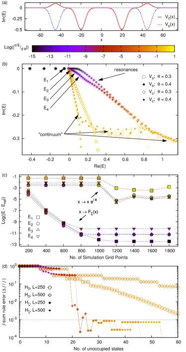
Figure 1: (a) 1D model potentials of Eq. (11). (b) Spectra obtained with different SESM tranformation, compared with the corresponding value of $\frac{\partial E}{\partial\theta}$ from Eq. (7). The simulation box considered has size $L=300$ AU. (c) SESM is compared against CSM for the Hamiltonian with $V_{s}$ potential. The error in the identification of some resonant energies (pointed by the arrows in panel (b)) is plotted against the number $N$ of degrees of freedom used in the simulation. Reference values are extracted with the SESM at $N=3000$. (d) Fulfillment of the $f$-sum rule for the $V_{c}$ potential as a function of the number of empty states considered for different $L$, ordered by $\left|\frac{\partial E}{\partial\theta}\right|$. Fermi level is chosen such as to have 8 occupied states.

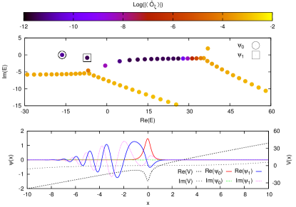
Figure 2: Measurement of $\langle\hat{O}_{\xi}\rangle$ from Eq. (9) for each state in the spectrum of a 1D “soft-Coulomb” potential with an external electric field. The parameters used are as in Fig. 2 of Ref. Larsen et al. (2013). We used the SESM Note (100), with $\theta=0.4$ and $x_{0}=12$, lying therefore outside the simulation box ($L=10$ AU). This enables us to extract the unscaled form of the true resonant eigenfunctions corresponding to the perturbation of the lowest bound states, indicated by $\psi_{0}$ and $\psi_{1}$.

As mentioned in the introduction, resonant states can be used to obtain a compact representation of the Green’s function. In systems with open boundaries, such a compact representation is very useful to express linear response functions and the derived optical spectroscopic properties in an optimal way. A good indicator of the quality of a discrete basis set for optical properties is the fulfillment of the Thomas-Reiche-Kuhn sum rule (or $f$-sum rule, see e.g. Ref. Baroni and Gebauer (2012)), which relates the first momentum of the oscillator strengths to that of the equilibrium density of the system, i.e. the number of states below the Fermi level. The information provided by Eq. (7) is of great utility in this case: we have plotted in Fig. 1 the fulfillment of the $f$-sum rule as a function of the number of unoccupied states considered, ordered by $\frac{\partial E}{\partial\theta}$, for the Hamiltonian with the $V_{c}$ potential. With such ordering, we are able to identify the minimal set of states allowing the fulfillment of the sum rule up to an excellent accuracy, independently of the simulation box size. This cannot be achieved with the low-energy eigenstates of the original, unscaled Hamiltonian, which suffer from the well-known continuum collapse Natarajan et al. (2012). Equivalent results can also be obtained by using the operator of Eq. (9).

Our approach can also be used to identify field-induced metastable states of Hamiltonians in non-trivial environments. A notable example of such metastability is given by the Stark ionization of molecules, recently studied within the framework of Density Functional Resonance Theory Whitenack and Wasserman (2011). The reliable determination of metastable states that have to be occupied is admittedly a problem in the latter treatment. However, our method provides a natural solution to this problem. As an example, in Fig. 2, we show the values of $\langle\hat{O}_{\xi}\rangle$ of Eq. (9) for a model Hamiltonian with a “soft-Coulomb” 1D potential under external electric field of intensity $\mathcal{E}$, see e.g. Ref. Larsen et al. (2013). States with smallest $|\langle\hat{O}_{\xi}\rangle|$ are those originating from a perturbation of the Rydberg states at $\mathcal{E}=0$, therefore not belonging to the set of “continuum” states of the SESM Hamiltonian. This approach would be very helpful in identifying the physical metastable channels of open quantum devices under external electric fields Goyer et al. (2007).

To summarize, we have presented a simple and robust method to numerically identify the Siegert states of open quantum systems undergoing a generic coordinate reparametrization. Such method, based on rigorous analytic derivations, makes the usage of rescaled Hamiltonians much more powerful than the artificial addition of ad hoc Complex Absorbing Potentials to the device. This method is especially useful for coordinate mappings leaving the potential of the quantum device unscaled, and does not require any finite-difference measurement of the eigenvalue sensitivity, avoiding the need of tracing trajectories in the parameter space and to search, graphically, for stable points. Our findings, supported by numerical examples with 1D model Hamiltonians, can straightforwardly be extended to 3D systems using e.g. separable forms of coordinate mappings Sajeev and Moiseyev (2007), and can be applied to any numerical basis set. The method provides scalar quantities enabling the identification of physically relevant states and, at the same time, indicates the reliability of the computational setup. We believe that our method paves the way for accurate investigations of scattering properties of open quantum systems. Work is in progress towards the iterative extraction of Siegert states out of non-Hermitian Hamiltonians.

The authors thank I. Duchemin for useful discussions.

References

- Gamow (1928) G. Gamow, Zeitschrift für Physik A Hadrons and Nuclei 51, 204 (1928), 10.1007/BF01343196.
- Berggren and Lind (1993) T. Berggren and P. Lind, Phys. Rev. C 47, 768 (1993).
- Sasada et al. (2011) K. Sasada, N. Hatano, and G. Ordonez, J.Phys.Soc.Jap. 80, 104707 (2011), arXiv:0905.3953 .
- Myo et al. (1998) T. Myo, A. Ohnishi, and K. Kato, Progress of Theoretical Physics 99, 801 (1998).
- Lind et al. (1994) P. Lind, R. J. Liotta, E. Maglione, and T. Vertse, Zeitschrift für Physik A Hadrons and Nuclei 347, 231 (1994).
- Tolstikhin et al. (1997) O. I. Tolstikhin, V. N. Ostrovsky, and H. Nakamura, Phys. Rev. Lett. 79, 2026 (1997).
- Moiseyev (2011) N. Moiseyev, Non-Hermitian Quantum Mechanics (Cambridge University Press, 2011).
- White et al. (2015) A. F. White, M. Head-Gordon, and C. W. McCurdy, The Journal of Chemical Physics 142, 054103 (2015).
- Rom et al. (1991) N. Rom, N. Lipkin, and N. Moiseyev, Chemical Physics 151, 199 (1991).
- Goyer et al. (2007) F. Goyer, M. Ernzerhof, and M. Zhuang, The Journal of Chemical Physics 126, 144104 (2007).
- Aguilar and Combes (1971) J. Aguilar and J. M. Combes, Communications in Mathematical Physics 22, 269 (1971).
- Cerioni et al. (2013) A. Cerioni, L. Genovese, I. Duchemin, and T. Deutsch, The Journal of Chemical Physics 138, 204111 (2013).
- Moiseyev (1998) N. Moiseyev, Journal of Physics B: Atomic, Molecular and Optical Physics 31, 1431 (1998).
- Sajeev and Moiseyev (2007) Y. Sajeev and N. Moiseyev, The Journal of Chemical Physics 127, 034105 (2007).
- Note (100) We use here , where , and .
- Larsen et al. (2013) A. H. Larsen, U. De Giovannini, D. L. Whitenack, A. Wasserman, and A. Rubio, The Journal of Physical Chemistry Letters 4, 2734 (2013).
- Baroni and Gebauer (2012) S. Baroni and R. Gebauer, in Fundamentals of Time-Dependent Density Functional Theory, Lecture Notes in Physics, Vol. 837, edited by M. A. Marques, N. T. Maitra, F. M. Nogueira, E. Gross, and A. Rubio (Springer Berlin Heidelberg, 2012) pp. 375–390.
- Natarajan et al. (2012) B. Natarajan, L. Genovese, M. E. Casida, T. Deutsch, O. N. Burchak, C. Philouze, and M. Y. Balakirev, Chemical Physics 402, 29 (2012).
- Whitenack and Wasserman (2011) D. Whitenack and A. Wasserman, Physical Review Letters 107, 1 (2011).