Assessing replicability of findings across two studies of multiple features

Abstract

Replicability analysis aims to identify the findings that replicated across independent studies that examine the same features. We provide powerful novel replicability analysis procedures for two studies for FWER and for FDR control on the replicability claims. The suggested procedures first select the promising features from each study solely based on that study, and then test for replicability only the features that were selected in both studies. We incorporate the plug-in estimates of the fraction of null hypotheses in one study among the selected hypotheses by the other study. Since the fraction of nulls in one study among the selected features from the other study is typically small, the power gain can be remarkable. We provide theoretical guarantees for the control of the appropriate error rates, as well as simulations that demonstrate the excellent power properties of the suggested procedures. We demonstrate the usefulness of our procedures on real data examples from two application fields: behavioural genetics and microarray studies.

1 Introduction

In modern science, it is often the case that each study screens many features. Identifying which of the many features screened have replicated findings, and the extent of replicability for these features, is of great interest. For example, the association of single nucleotide polymorphisms (SNPs) with a phenotype is typically considered a scientific finding only if it has been discovered in independent studies, that examine the same associations with phenotype, but on different cohorts, with different environmental exposures (Heller et al., 2014a, ).

Two studies that examine the same problem may only partially agree on which features have signal. For example, in the two microarray studies discussed in Section 8.2, among the 22283 probes examined in each study we estimated that 29% have signal in both studies, but 32% have signal in exactly one of the studies. Possible explanations for having signal in only one of the studies include bias (e.g., in the cohorts selected or in the laboratory process), and the fact that the null hypotheses tested may be too specific (e.g., to the specific cohorts that were subject to specific exposures in a each study). In a typical meta-analysis, all the features with signal in at least one of the studies are of interest (estimated to be 61% of the probes in our example). However, the subset of the potential meta-analysis findings which have signal in both studies may be of particular interest, for both verifiability and generalizability of the results. Replicability analysis targets this subset, and aims to identify the features with signal in both studies (estimated to be 29% of the probes in our example).

Formal statistical methods for assessing replicability, when each study examines many features, were developed only recently. An empirical Bayes approach for two studies was suggested by Li et al., (2014), and for at least two studies by Heller and Yekutieli, (2014). The accuracy of the empirical Bayes analysis relies on the ability to estimate well the unknown parameters, and thus it may not be suitable for applications with a small number of features and non-local dependency in the measurements across features. A frequentist approach was suggested in Benjamini et al., (2009), which suggested applying the Benjamini-Hochberg (BH) procedure (Benjamini and Hochberg,, 1995) to the maximum of the two studies $p$-values. However, Heller and Yekutieli, (2014) and Bogomolov and Heller, (2013) noted that the power of this procedure may be low when there is nothing to discover in most features. Bogomolov and Heller, (2013) suggested instead applying twice their procedures for establishing replicability from a primary to a follow-up study, where each time one of the studies takes on the role of a primary study and the other the role of the follow-up study.

In this work we suggest novel procedures for establishing replicability across two studies, which are especially useful in modern applications when the fraction of features with signal is small (e.g., the approaches of Bogomolov and Heller, (2013) and Benjamini et al., (2009) will be less powerful whenever the fraction of features with signal is smaller than half). The advantage of our procedures over previous ones is due to two main factors. First, these procedures are based on our novel approach, which selects the promising features from each study solely based on that study, and then tests for replicability only the features that were selected in both studies. This approach focuses attention on the promising features, and has the added advantage of reducing the number of features that need to be accounted for in the subsequent replicability analysis. Note that since the selection is only a first step, it may be much more liberal than that made by a multiple testing procedure, and can include all features that seem interesting to the investigator (see Remark 3.2 for a discussion of selection by multiple testing). Second, we incorporate in our procedures estimates of the fraction of nulls in one study among the features selected in the other study. We show that exploiting these estimates can lead to far more replicability claims while still controlling the relevant error measures. For single studies, multiple testing procedures that incorporate estimates of the fraction of nulls, i.e. the fraction of features in which there is nothing to discover, are called adaptive procedures (Benjamini and Hochberg,, 2000) or plug-in procedures (Finner and Gontsharuk,, 2009). One of the simplest, and still very popular, estimators is the plug-in estimator, reviewed in Section 1.1. The smaller is the fraction of nulls, the higher is the power gain due to the use of the plug-in estimator. In this work, there is a unique opportunity for using adaptivity: even if the fraction of nulls in each individual study is close to one, the fraction of nulls in study one (two) among the selected features based on study two (one) may be small since the selected features are likely to contain mostly features with false null hypotheses in both studies. In the data examples we consider, the fraction of nulls in one study among the selected in the other study was lower than 50%, and we show in simulations that the power gain from adaptivity can be large.

Our procedures also report the strength of the evidence towards replicability by a number for each outcome, the $r$-value for replicability, introduced in Heller et al., 2014a and reviewed in Section 2. The remaining of the paper is organized as follows. In Section 2 we describe the formal mathematical framework. We introduce our new non-adaptive FWER- and FDR-replicability analysis procedures in Section 3, and their adaptive variants in Section 4. For simplicity, we shall present the notation, procedures, and theoretical results for one-sided hypotheses tests in Sections 2-4. In Section 5 we present the necessary modifications for two-sided hypotheses, which turn out to be minimal. In Section 6 we suggest selection rules with optimal properties. In Sections 7 and 8 we present a simulation study and real data examples, respectively. Conclusions are given in Section 9. Lengthy proofs of theoretical results are in the Appendix.

1.1 Review of the plug-in estimator for estimating the fraction of nulls

Let $\pi_{0}$ be the fraction of null hypotheses. Schweder and Spjotvoll, (1982) proposed estimating this fraction by $\frac{\#\{p-values>\lambda\}}{m(1-\lambda)},$ where $m$ is the number of features and $\lambda\in(0,1)$. The slightly inflated plug-in estimator

$$\hat{\pi}_{0}=\frac{\#\{p-values>\lambda\}+1}{m(1-\lambda)}$$

has been incorporated into multiple testing procedures in recent years. For independent $p$-values, Storey, (2003) proved that applying the BH procedure with $m\hat{\pi}_{0}$ instead of $m$ controls the FDR, and Finner and Gontsharuk, (2009) proved that applying Bonferroni with $m\hat{\pi}_{0}$ instead of $m$ controls the FWER.

Adaptive procedures in single studies have larger power gain over non-adaptive procedures when the fraction of nulls, $\pi_{0}$, is small. This is so because these procedures essentially apply the original procedure at level $1/\hat{\pi}_{0}$ times the nominal level to achieve FDR or FWER control at the nominal level. Finner and Gontsharuk, (2009) showed in simulations that the power gain of using $m\hat{\pi}_{0}$ instead of $m$ can be small when the fraction of nulls is 60%, but large when the fraction of nulls is 20%.

The plug-in estimator is typically less conservative (smaller) the larger $\lambda$ is. This follows from Lemma 1 in Dickhaus et al., (2012), that showed that for a single study the estimator is biased upwards, and that the bias is a decreasing function of $\lambda$ if the cumulative distribution function (CDF) of the non-null $p$-values is concave (if the $p$-values are based on a test statistic whose density is eventually strictly decreasing, then concavity will hold, at least for small $\lambda$). Benjamini et al., (2006) noted that the FDR of the BH procedure which incorporates the plug-in estimator with $\lambda=0.5$ is sensitive to deviations from the assumption of independence, and it may be inflated above the nominal level under dependency. Blanchard and Roquain, (2009) further noted that although under equi-correlation among the test statistics using the plug-in estimators does not control the FDR with $\lambda=0.5$, it does control the FDR with $\lambda=q/(q+1+1/m)\approx q$. Blanchard and Roquain, (2009) compared in simulations with dependent test statistics the adaptive BH procedure using various estimators of the fraction of nulls for single studies, including the plug-in estimator with $\lambda\in\{0.05,0.5\}$. Their conclusion was that the plug-in estimator with $\lambda=0.05$ was superior to all other estimators considered, since it had the highest power overall without inflating the FDR above the 0.05 nominal level.

2 Notation, goal, and review for replicability analysis

Consider a family of $m$ features examined in two independent studies. The effect of feature $j\in\{1,\ldots,m\}$ in study $i\in\{1,2\}$ is $\theta_{ij}$. Let $H_{ij}$ be the hypothesis indicator, so $H_{ij}=0$ if $\theta_{ij}=\theta_{ij}^{0}$, and $H_{ij}=1$ if $\theta_{ij}>\theta_{ij}^{0}$.

Let $\vec{H}_{j}=(H_{1j},H_{2j})$. The set of possible states of $\vec{H}_{j}$ is $\mathcal{H}=\{\vec{h}=(h_{1},h_{2}):(0,0),(1,0),(0,1),(1,1)\}.$ The goal of inference is to discover as many features as possible with $\vec{H}_{j}\notin\mathcal{H}^{0}$, where $\mathcal{H}^{0}\subset\mathcal{H}.$ For replicability analysis, $\mathcal{H}^{0}=\mathcal{H}^{0}_{NR}=\{(0,0),(0,1),(1,0)\}$. For a typical meta-analysis, $\mathcal{H}^{0}=\{(0,0)\}$, and the number of features with state $(0,0)$ can be much smaller than the number of features with states in $\mathcal{H}^{0}_{NR}$, see the example in Section 8.2.

We aim to discover as many features with $\vec{H}_{j}=(1,1)$ as possible, i.e., true replicability claims, while controlling for false replicability claims, i.e. replicability claims for features with $\vec{H}_{j}\in\mathcal{H}^{0}_{NR}.$ Let $\mathcal{R}$ be the set of indices of features with replicability claims. The FWER and FDR for replicability analysis are defined as follows:

$$FWER=\textmd{Pr}\left(|\mathcal{R}\cap\{j:\vec{H}_{j}\in\mathcal{H}^{0}_{NR}\}|>0\right),\quad FDR=E\left(\frac{|\mathcal{R}\cap\{j:\vec{H}_{j}\in\mathcal{H}^{0}_{NR}\}|}{\max(|\mathcal{R}|,1)}\right),$$

where $E(\cdot)$ is the expectation.

Our novel procedures first select promising features from each study solely based on the data of that study. Let $\mathcal{S}_{i}$ be the index set of features selected in study $i,$ for $i\in\{1,2\},$ and let $S_{i}=|\mathcal{S}_{i}|$ be their number. The procedures proceed towards making replicability claims only on the index set of features which are selected in both studies, i.e. $\mathcal{S}_{1}\cap\mathcal{S}_{2}.$ For example, selected sets may include all (or a subset of) features with two-sided $p$-values below $\alpha$. See Remark 3.2 for a discussion about the selection process.

Let $P_{i}=(P_{i1},\ldots,P_{im})$ be the $m$-dimensional random vector of $p$-values of study $i\in\{1,2\},$ and $p_{i}=(p_{i1},\ldots,p_{im})$ be its realization. We shall assume the following condition is satisfied for $(P_{1},P_{2})$:

Definition 2.1.

The studies satisfy the null independence-across-studies condition if for all $j$ with $\vec{H}_{j}\in\mathcal{H}^{0}_{NR}$, if $H_{1j}=0$ then $P_{1j}$ is independent of $P_{2}$, and if $H_{2j}=0$ then $P_{2j}$ is independent of $P_{1}$.

This condition is clearly satisfied if the two studies are independent, but it also allows the pairs $(P_{1j},P_{2j})$ to be dependent for $\vec{H}_{j}\notin\mathcal{H}^{0}_{NR}$. Note moreover that this condition does not pose any restriction on the joint distribution of $p$-values within each study.

We shall assess the evidence towards replicability by a quantity we call the $r$-value, introduced in Heller et al., 2014a , which is the adjusted $p$-value for replicability analysis. In a single study, the adjusted $p$-value of a feature is the smallest level (of FWER or FDR) at which it is discovered (Wright,, 1992). Similarly, for feature $j$, the $r$-value is the smallest level (of FWER or FDR) at which feature $j$ is declared replicable.

The simplest example of $p$-value adjustment for a single study $i\in\{1,2\}$ is Bonferroni, with adjusted $p$-values $p_{ij}^{adj-Bonf}=mp_{ij},j=1,\ldots,m$. The BH adjusted $p$-values build upon the Bonferroni adjusted $p$-values (Reiner et al.,, 2003). The BH adjusted $p$-value for feature $j$ is defined to be

$$\min_{\{k:\,p_{ik}^{adj-Bonf}\geq p_{ij}^{adj-Bonf},\,k=1,\ldots,m\}}\frac{p_{ik}^{adj-Bonf}}{rank(p_{ik}^{adj-Bonf})},$$

where $rank(p_{ik}^{adj-Bonf})$ is the rank of the Bonferroni adjusted $p$-value for feature $k$, with maximum rank for ties. For two studies, we can for example define the Bonferroni-on-max $r$-values to be $r_{j}^{Bonf-max}=m\max(p_{1j},p_{2j}),j=1,\ldots,m$. The BH-on-max $r$-values build upon the Bonferroni-on-max $r$-values exactly as in single studies. The BH-on-max $r$-value for feature $j$ is defined to be

$$\min_{\{k:\,r_{k}^{Bonf-max}\geq r_{j}^{Bonf-max},\,k=1,\ldots,m\}}\frac{r_{k}^{Bonf-max}}{rank(r_{k}^{Bonf-max})},$$

where $rank(r_{k}^{Bonf-max})$ is the rank of the Bonferroni-on-max adjusted $p$-value for feature $k$, with maximum rank for ties. Claiming as replicable the findings of all features with BH-on-max $r$-values at most $\alpha$ is equivalent to considering as replicability claims the discoveries from applying the BH procedure at level $\alpha$ on the maximum of the two studies $p$-values, suggested in Benjamini et al., (2009). In this work we introduce $r$-values that are typically much smaller than the above-mentioned $r$-values for features selected in both studies, with the same theoretical guarantees upon rejection at level $\alpha$, and thus preferred for replicability analysis of two studies.

3 Replicability among the selected in each of two studies

Let $c\in(0,1)$, with default value $c=0.5$, be the fraction of the significance level “dedicated” to study one. The Bonferroni $r$-values are

$$r^{Bonf}_{j}=\max\left(\frac{S_{2}p_{1j}}{c},\frac{S_{1}p_{2j}}{1-c}\right),\quad j\in\mathcal{S}_{1}\cap\mathcal{S}_{2}.$$

The FDR $r$-values build upon the Bonferroni $r$-values and are necessarily smaller:

$$r^{FDR}_{j}=\min_{\{i:\,r^{Bonf}_{i}\geq r^{Bonf}_{j},\,i\in\mathcal{S}_{1}\cap\mathcal{S}_{2}\}}\frac{r^{Bonf}_{i}}{rank(r^{Bonf}_{i})},\quad j\in\mathcal{S}_{1}\cap\mathcal{S}_{2}.$$ (3.1)

where $rank(r^{Bonf}_{i})$ is the rank of the Bonferroni $r$-value for feature $i\in\mathcal{S}_{1}\cap\mathcal{S}_{2}$, with maximum rank for ties.

Declaring as replicated all features with Bonferroni $r$-values at most $\alpha$ controls the FWER at level $\alpha$, and declaring as replicated all features with FDR $r$-values at most $\alpha$ controls the FDR at level $\alpha$ under independence, see Section 3.1.

The relation between the Bonferroni and FDR $r$-values is similar to that of the adjusted Bonferroni and adjusted BH $p$-values described in Section 2. For the features selected in both studies, if less than half of the features are selected by each study, it is easy to show that FDR (Bonferroni) $r$-values given above, using $c=0.5$, will be smaller than (1) the BH-on-max (Bonferroni-on-max) $r$-values described in Section 2, and (2) the $r$-values that correspond to the FDR-controlling symmetric procedure in Bogomolov and Heller, (2013), which will be typically smaller than BH-on-max $r$-values but larger than FDR $r$-values in (3.1) due to taking into account the multiplicity of all features considered.

3.1 Theoretical properties

Let $\alpha\in(0,1)$ be the level of control desired, e.g. $\alpha=0.05$. Let $\alpha_{1}=c\alpha$ be the fraction of $\alpha$ for study one, e.g. $\alpha_{1}=\alpha/2$.

The procedure that makes replicability claims for features with Bonferroni $r$-values at most $\alpha$ is a special case of the following more general procedure.

Procedure 3.1.

FWER-replicability analysis on the selected features $\mathcal{S}_{1}\cap\mathcal{S}_{2}$:

1. Apply a FWER controlling procedure at level $\alpha_{1}$ on the set $\{p_{1j},j\in\mathcal{S}_{2}\},$ and let $\mathcal{R}_{1}$ be the set of indices of discovered features. Similarly, apply a FWER controlling procedure at level $\alpha-\alpha_{1}$ on the set $\{p_{2j},j\in\mathcal{S}_{1}\},$ and let $\mathcal{R}_{2}$ be the set of indices of discovered features.

2. The set of indices of features with replicability claims is $\mathcal{R}_{1}\cap\mathcal{R}_{2}$.

When using Bonferroni in Procedure 3.1, feature $j\in\mathcal{S}_{1}\cap\mathcal{S}_{2}$ is among the discoveries if and only if $(p_{1j},p_{2j})\leq(\alpha_{1}/S_{2},\quad(\alpha-\alpha_{1})/S_{1}).$ Therefore, claiming replicability for all features with Bonferroni $r$-values at most $\alpha$ is equivalent to Procedure 3.1 using Bonferroni.

Theorem 3.1.

If the null independence-across-studies condition is satisfied, then Procedure 3.1 controls the FWER for replicability analysis at level $\alpha$.

Proof.

Let $V_{1}=|\mathcal{R}_{1}\cap\{j:H_{1j}=0\}|$ and $V_{2}=|\mathcal{R}_{2}\cap\{j:H_{2j}=0\}|$ be the number of true null hypotheses rejected in study one and in study two, respectively, by Procedure 3.1. Then the FWER for replicability analysis is

$$E(\textbf{I}[V_{1}+V_{2}>0])\leq E(E(\textbf{I}[V_{1}>0]|P_{2}))+E(E(\textbf{I}[V_{2}>0]|P_{1})).$$

Clearly, $E(\textbf{I}[V_{1}>0]|P_{2})\leq\alpha_{1}$ since $P_{1j}$ is independent of $P_{2}$ for all $j$ with $H_{1j}=0$, and a FWER controlling procedure is applied on $\{p_{1j},j\in\mathcal{S}_{2}\}.$ Similarly, $E(\textbf{I}[V_{2}>0]|P_{1})\leq\alpha-\alpha_{1}$. It thus follows that the FWER for replicability analysis is at most $\alpha$. ∎

The procedure that rejects the features with FDR $r$-values at most $\alpha$ is equivalent to the following procedure, see Lemma B.1 for a proof.

Procedure 3.2.

FDR-replicability analysis on the selected features $\mathcal{S}_{1}\cap\mathcal{S}_{2}$:

1. Let

   $$R\triangleq\max\left\{r:\sum_{j\in\mathcal{S}_{1}\cap\mathcal{S}_{2}}\textbf{I}\left[(p_{1j},p_{2j})\leq\left(\frac{r\alpha_{1}}{S_{2}},\frac{r(\alpha-\alpha_{1})}{S_{1}}\right)\right]=r\right\}.$$

2. The set of indices with replicability claims is

   $$\mathcal{R}=\{j:(p_{1j},p_{2j})\leq\left(\frac{R\alpha_{1}}{S_{2}},\frac{R(\alpha-\alpha_{1})}{S_{1}}\right),j\in\mathcal{S}_{1}\cap\mathcal{S}_{2}\}.$$

This procedure controls the FDR for replicability analysis at level $\alpha$ as long as the selection rules by which the sets $\mathcal{S}_{1}$ and $\mathcal{S}_{2}$ are selected are stable (this is a very lenient requirement, see Bogomolov and Heller, (2013) for examples).

Definition 3.1.

(Bogomolov and Heller,, 2013) A stable selection rule satisfies the following condition: for any selected feature, changing its $p$-value so that the feature is still selected while all other $p$-values are held fixed, will not change the set of selected features.

Theorem 3.2.

If the null independence-across-studies condition is satisfied, and the selection rules by which the sets $\mathcal{S}_{1}$ and $\mathcal{S}_{2}$ are selected are stable, then Procedure 3.2 controls the FDR for replicability analysis at level $\alpha$ if one of the following items is satisfied:

1. The $p$-values from true null hypotheses within each study are each independent of all other $p$-values.

2. Arbitrary dependence among the $p$-values within each study, when $S_{i}$ in Procedure 3.2 is replaced by $S_{i}\sum_{k=1}^{S_{i}}1/k$, for $i=1,2$.

See Appendix B for a proof.

Remark 3.1.

The FDR $r$-values for the procedure that is valid for arbitrary dependence, denoted by $\tilde{r}_{j}^{FDR},j\in\mathcal{S}_{1}\cap\mathcal{S}_{2}$, are computed using formula (3.1) where the Bonferroni $r$-values $r_{j}^{Bonf}$ are replaced by

$$\tilde{r}_{j}=\max\left(\frac{(\sum_{i=1}^{S_{2}}1/i)S_{2}p_{1j}}{c},\frac{(\sum_{i=1}^{S_{1}}1/i)S_{1}p_{2j}}{1-c}\right),\quad j\in\mathcal{S}_{1}\cap\mathcal{S}_{2}.$$ (3.2)

Remark 3.2.

An intuitive approach towards replicability may be to apply a multiple testing procedure on each study separately, with discovery sets $\mathcal{D}_{1}$ and $\mathcal{D}_{2}$ in study one and two, respectively, and then claim replicability on the set $\mathcal{D}_{1}\cap\mathcal{D}_{2}$. However, even if the multiple testing procedure has guaranteed FDR control at level $\alpha$, it is easy to construct examples where the expected fraction of false replicability claims in $\mathcal{D}_{1}\cap\mathcal{D}_{2}$ will be far larger than $\alpha$. An extreme example is the following: half of the features have $\vec{H}_{j}=(1,0)$, the remaining half have $\vec{H}_{j}=(0,1)$, and the signal is very strong. Then in study one all features with $\vec{H}_{j}=(1,0)$ and few features with $\vec{H}_{j}=(0,1)$ will be discovered, and in study two all features with $\vec{H}_{j}=(0,1)$ and few features with $\vec{H}_{j}=(1,0)$ will be discovered, resulting in a non-empty set $\mathcal{D}_{1}\cap\mathcal{D}_{2}$ which contains only false replicability claims. Interestingly, if the multiple testing procedure is Bonferroni at level $\alpha$, then the FWER on replicability claims of the set $\mathcal{D}_{1}\cap\mathcal{D}_{2}$ is at most $\alpha$. However, this procedure (which can be viewed as Bonferroni on the maximum of the two study $p$-values) can be far more conservative than our suggested Bonferroni-type procedure. If we select in each study separately all features with $p$-values below $\alpha/2$, resulting in selection sets $\mathcal{S}_{1}$ and $\mathcal{S}_{2}$ in study one and two, respectively, then using our Bonferroni-type procedure we claim replicability for features with $(p_{1j},p_{2j})\leq(\alpha/(2S_{2}),\alpha/(2S_{1}))$. Our discovery thresholds, $(\alpha/(2S_{2}),\alpha/(2S_{1}))$, are both larger than $\alpha/m$ as long as the number of features selected by each study is less than half, and thus can lead to more replicability claims with FWER control at level $\alpha$.

4 Incorporating the plug-in estimates

When the non-null hypotheses are mostly non-null in both studies, i.e., there are more features with $\vec{H}_{j}=(1,1)$ than with $\vec{H}_{j}=(1,0)$ or $\vec{H}_{j}=(0,1)$, then the non-adaptive procedures for replicability analysis may be over conservative. The conservativeness follows from the fact that the fraction of null hypotheses in one study among the selected in the other study is small. The set $\mathcal{S}_{1}$ is more likely to contain hypotheses with $\vec{H}_{j}\in\{(1,0),(1,1)\}$ than hypotheses with $\vec{H}_{j}\in\{(0,0),(0,1)\},$ and therefore the fraction of true null hypotheses in study two among the selected in study one, i.e., $\sum_{j\in\mathcal{S}_{1}}(1-H_{2j})/S_{1}$, may be much smaller than one (especially if there are more features with $\vec{H}_{j}=(1,1)$ than with $\vec{H}_{j}=(1,0)$). Similarly, the fraction of true null hypotheses in study one among the selected based on study two, i.e., $\sum_{j\in\mathcal{S}_{2}}(1-H_{1j})/S_{2}$, may be much smaller than one.

The non-adaptive procedures for replicability analysis in Section 3 control the error-rates at levels that are conservative by the expectation of these fractions. Procedures 3.1 using Bonferroni and 3.2 control the FWER and FDR, respectively, at level which is at most

$$\alpha_{1}E\left(\frac{\sum_{j\in\mathcal{S}_{2}}(1-H_{1j})}{S_{2}}\right)+(\alpha-\alpha_{1})E\left(\frac{\sum_{j\in\mathcal{S}_{1}}(1-H_{2j})}{S_{1}}\right),$$

which can be much smaller than $\alpha$ if the above expectations are far smaller than one. This upper bound follows for FWER since an upper bound for the FWER of a Bonferroni procedure is the desired level times the fraction of null hypotheses in the family tested, and for the FDR from the proof of item 1 of Theorem 3.2.

We therefore suggest adaptive variants, that first estimate the expected fractions of true null hypotheses among the selected. We use the slightly inflated plug-in estimators (reviewed in Section 1.1):

$$\hat{\pi}_{0}^{{I}}=\frac{1+\sum_{j\in\mathcal{S}_{2,\lambda}}\textbf{I}(P_{1j}>\lambda)}{S_{2,\lambda}(1-\lambda)};\,\,\,\hat{\pi}_{0}^{{II}}=\frac{1+\sum_{j\in\mathcal{S}_{1,\lambda}}\textbf{I}(P_{2j}>\lambda)}{S_{1,\lambda}(1-\lambda)},$$ (4.1)

where $0<\lambda<1$ is a fixed parameter, $\mathcal{S}_{i,\lambda}=\mathcal{S}_{i}\cap\{j:P_{ij}\leq\lambda\}$, and $S_{i,\lambda}=|\mathcal{S}_{i,\lambda}|$, for $i=1,2$. Although $\hat{\pi}_{0}^{{I}}$ and $\hat{\pi}_{0}^{{II}}$ depend on the tuning parameter $\lambda,$ we suppress the dependence of the estimates on $\lambda$ for ease of notation.

The adaptive Bonferroni $r$-values for fixed $c=\alpha_{1}/\alpha$ are:

$$r^{adaptBonf}_{j}=\max\left(\frac{\hat{\pi}_{0}^{{I}}S_{2,\lambda}p_{1j}}{c},\frac{\hat{\pi}_{0}^{{II}}S_{1,\lambda}p_{2j}}{1-c}\right),\quad j\in\mathcal{S}_{1,\lambda}\cap\mathcal{S}_{2,\lambda}.$$

As in Section 3, the adaptive FDR $r$-values build upon the adaptive Bonferroni $r$-values:

$$r^{adaptFDR}_{j}=\min_{\{i:\,r^{adaptBonf}_{i}\geq r^{adaptBonf}_{j},\,i\in\mathcal{S}_{1,\lambda}\cap\mathcal{S}_{2,\lambda}\}}\frac{r^{adaptBonf}_{i}}{rank(r^{adaptBonf}_{i})},\quad j\in\mathcal{S}_{1,\lambda}\cap\mathcal{S}_{2,\lambda}$$

where $rank(r^{adaptBonf}_{i})$ is the rank of the adaptive Bonferroni $r$-value for feature $i\in\mathcal{S}_{1,\lambda}\cap\mathcal{S}_{2,\lambda}$, with maximum rank for ties. Declaring as replicated all features with adaptive Bonferroni/FDR $r$-values at most $\alpha$ controls the FWER/FDR for replicability analysis at level $\alpha$ under independence, see Section 4.1.

The non-adaptive procedures in Section 3 only require as input $\{p_{1j}:j\in\mathcal{S}_{1}\}$ and $\{p_{2j}:j\in\mathcal{S}_{2}\}$. However, if $\{p_{1j}:j\in\mathcal{S}_{1}\cup\mathcal{S}_{2}\}$ and $\{p_{2j}:j\in\mathcal{S}_{1}\cup\mathcal{S}_{2}\}$ are available, then the adaptive procedures with $\lambda=\alpha$ are attractive alternatives with better power, as demonstrated in our simulations detailed in Section 7.

4.1 Theoretical properties

The following Procedure 4.1 is equivalent to declaring as replicated all features with Bonferroni adaptive $r$-values at most $\alpha$.

Procedure 4.1.

Adaptive-Bonferroni-replicability analysis on $\{(p_{1j},p_{2j}):j\in\mathcal{S}_{1}\cup S_{2}\}$ with input parameter $\lambda$:

1. Compute $\hat{\pi}_{0}^{{I}},\hat{\pi}_{0}^{{II}}$ and $S_{1,\lambda},S_{2,\lambda}$.

2. Let $\mathcal{R}_{1}=\{j\in\mathcal{S}_{1,\lambda}:p_{1j}\leq\alpha_{1}/(S_{2,\lambda}\hat{\pi}_{0}^{{I}})\}$ and $\mathcal{R}_{2}=\{j\in\mathcal{S}_{2,\lambda}:p_{2j}\leq(\alpha-\alpha_{1})/(S_{1,\lambda}\hat{\pi}_{0}^{{II}})\}$ be the sets of indices of features discovered in studies one and two, respectively.

3. The set of indices of features with replicability claims is $\mathcal{R}_{1}\cap\mathcal{R}_{2}$.

Theorem 4.1.

If the null independence-across-studies condition is satisfied, and the $p$-values from true null hypotheses within each study are jointly independent, then Procedure 4.1 controls the FWER for replicability analysis at level $\alpha$.

Proof.

It is enough to prove that $E(\textbf{I}[V_{1}>0]|P_{2})\leq\alpha_{1}$ and $E(\textbf{I}[V_{2}>0]|P_{1})\leq\alpha-\alpha_{1},$ as we showed in the proof of Theorem 3.1. These inequalities essentially follow from the fact that the Bonferroni plug-in procedure controls the FWER (Finner and Gontsharuk,, 2009). We will only show that $E(\textbf{I}[V_{1}>0]|P_{2})\leq\alpha_{1}$, since the proof that $E(\textbf{I}[V_{2}>0]|P_{1})\leq\alpha-\alpha_{1}$ is similar. We shall use the fact that

$$\hat{\pi}_{0}^{{I}}\geq\frac{1+\sum_{j\in\mathcal{S}_{2,\lambda}}(1-H_{1j})\textbf{I}(P_{1j}>\lambda)}{S_{2,\lambda}(1-\lambda)}.$$ (4.2)

$$E(\textbf{I}[V_{1}>0]|P_{2})=\textmd{Pr}\left(\sum_{i\in\mathcal{S}_{2,\lambda}}(1-H_{1i})\textbf{I}[i\in S_{1,\lambda},P_{1i}\leq\alpha_{1}/(S_{2,\lambda}\hat{\pi}_{0}^{{I}})]>0|P_{2}\right)$$

$$\leq\sum_{i\in\mathcal{S}_{2,\lambda}}(1-H_{1i})\textmd{Pr}(P_{1i}\leq\min(\lambda,\alpha_{1}/S_{2,\lambda}\hat{\pi}_{0}^{{I}})|P_{2})$$ (4.3)

$$\leq\sum_{i\in\mathcal{S}_{2,\lambda}}(1-H_{1i})\textmd{Pr}\left(P_{1i}\leq\min\left(\lambda,\frac{\alpha_{1}}{\left(\frac{1+\sum_{j\in\mathcal{S}_{2,\lambda}}(1-H_{1j})\textbf{I}(P_{1j}>\lambda)}{1-\lambda}\right)}\right)|P_{2}\right)$$ (4.4)

$$=\sum_{i\in\mathcal{S}_{2,\lambda}}(1-H_{1i})\textmd{Pr}\left(P_{1i}\leq\min\left(\lambda,\frac{\alpha_{1}}{\left(\frac{1+\sum_{j\in\mathcal{S}_{2,\lambda},j\neq i}(1-H_{1j})\textbf{I}(P_{1j}>\lambda)}{1-\lambda}\right)}\right)|P_{2}\right)$$

$$\leq\sum_{i\in\mathcal{S}_{2,\lambda}}(1-H_{1i})\alpha_{1}E\left(1/\left(\frac{1+\sum_{j\in\mathcal{S}_{2,\lambda},j\neq i}(1-H_{1j})\textbf{I}(P_{1j}>\lambda)}{1-\lambda}\right)|P_{2}\right)$$ (4.5)

$$\leq\sum_{i\in\mathcal{S}_{2,\lambda}}(1-H_{1i})\alpha_{1}/\sum_{j\in\mathcal{S}_{2,\lambda}}(1-H_{1j})=\alpha_{1}.$$ (4.6)

Inequality (4.3) follows from the Bonferroni inequality, and inequality (4.4) follows from (4.2). Inequality (4.5) follows from the facts that for $i$ with $H_{1i}=0$, (a) $P_{1i}$ is independent of all null $p$-values from study one and from all $p$-values from study two, and (b) $\textmd{Pr}(P_{1i}\leq x)\leq x$ for all $x\in[0,1].$ Inequality (4.6) follows by applying Lemma 1 in Benjamini et al., (2006), which states that if $Y\sim B(k-1,p)$ then $E(1/(Y+1))<1/(kp)$, to $Y=\sum_{j\in\mathcal{S}_{2,\lambda},j\neq i}(1-H_{1j})\textbf{I}(P_{1j}>\lambda)$, which is distributed $B(\sum_{j\in\mathcal{S}_{2,\lambda},j\neq i}(1-H_{1j}),1-\lambda)$ if the null $p$-values within each study are uniformly distributed. It is easy to show, using similar arguments, that inequality (4.6) remains true when the null $p$-values are stochastically larger than uniform. ∎

Declaring as replicated all features with adaptive FDR $r$-values at most $\alpha$ is equivalent to Procedure 3.2 where $S_{1}$ and $S_{2}$ are replaced by $S_{1,\lambda}\hat{\pi}_{0}^{{II}}$ and $S_{2,\lambda}\hat{\pi}_{0}^{{I}}$ respectively, and $\mathcal{S}_{1}\cap\mathcal{S}_{2}$ is replaced by $\mathcal{S}_{1,\lambda}\cap\mathcal{S}_{2,\lambda},$ see Lemma B.1 for a proof.

Theorem 4.2.

If the null independence-across-studies condition holds, the $p$-values corresponding to true null hypotheses are each independent of all the other $p$-values, and the selection rules by which the sets $\mathcal{S}_{1}$ and $\mathcal{S}_{2}$ are selected are stable, then declaring as replicated all features with adaptive FDR $r$-values at most $\alpha$ controls the FDR for replicability analysis at level $\alpha$.

See Appendix B for a proof.

5 Directional replicability analysis for two-sided alternatives

So far we have considered one sided alternatives. If a two-sided alternative is considered for each feature in each study, and the aim is to discover the features that have replicated effect in the same direction in both studies, the following simple modifications are necessary.

For feature $j\in\{1,\ldots,m\}$, the left- and right- sided $p$-values for study $i\in\{1,2\}$ are denoted by $p^{L}_{ij}$ and $p^{R}_{ij}$, respectively. For continuous test statistics, $p^{R}_{ij}=1-p^{L}_{ij}$.

For directional replicability analysis, the selection step has to be modified to include also the selection of the direction of testing. The set of features selected is the subset of features that are selected from both studies, for which the direction of the alternative with the smallest one-sided $p$-value is the same for both studies, i.e.,

$$\mathcal{S}\triangleq\mathcal{S}_{1}\cap\mathcal{S}_{2}\cap\left(\{j:\max(p_{1j}^{R},p_{2j}^{R})<0.5\}\cup\{j:\max(p_{1j}^{L},p_{2j}^{L})<0.5\}\right).$$

In addition, define for $j\in\mathcal{S}_{1}\cup\mathcal{S}_{2},$

$$p^{\prime}_{1j}=\left\{\begin{array}[]{rl}p_{1j}^{L}&\text{if }p_{2j}^{L}<p_{2j}^{R},\\ p_{1j}^{R}&\text{if }p_{2j}^{L}>p_{2j}^{R},\end{array}\right.$$

$$p^{\prime}_{2j}=\left\{\begin{array}[]{rl}p_{2j}^{L}&\text{if }p_{1j}^{L}<p_{1j}^{R},\\ p_{2j}^{R}&\text{if }p_{1j}^{L}>p_{1j}^{R}.\end{array}\right.$$

The Bonferroni and FDR $r$-values are computed for features in $\mathcal{S}$ using the formulae given in Sections 3 and 4 (where $\mathcal{S}_{1,\lambda}$ and $\mathcal{S}_{2,\lambda}$ are the selected sets in Section 4), with the following modifications: the set $\mathcal{S}_{1}\cap\mathcal{S}_{2}$ is replaced by $\mathcal{S}$, and $p_{1j}$ and $p_{2j}$ are replaced by $p^{\prime}_{1j}$ and $p^{\prime}_{2j}$ for $j\in\mathcal{S}_{1}\cup\mathcal{S}_{2}.$

As in Sections 3 and 4, features with $r$-values at most $\alpha$ are declared as replicated at level $\alpha$, in the direction selected. The corresponding procedures remain valid, with the theoretical guarantees of directional FWER and FDR control for replicability analysis on the modified selected set above, despite the fact that the direction of the alternative for establishing replicability was not known in advance. This is remarkable, since it means that there is no additional penalty, beyond the penalty for selection used already in the above procedures, for the fact that the direction for establishing replicability is also decided upon selection. The proofs are similar to the proofs provided for one-sided hypotheses and are therefore omitted.

6 Estimating the selection thresholds

When the full data for both studies is available, we first need to select the promising features from each study based on the data in this study. If the selection is based on $p$-values, then our first step will include selecting the features with $p$-values below thresholds $t_{1}$ and $t_{2}$ for studies one and two, respectively. The thresholds for selection, $(t_{1},t_{2})\in(0,1]^{2}$, affect power: if $(t_{1},t_{2})$ are too low, features with $\vec{H}_{j}\notin\mathcal{H}^{0}_{NR}$ may not be considered for replicability even if they have a chance of being discovered upon selection, thus resulting in power loss; if $(t_{1},t_{2})$ are too high, too many features with $\vec{H}_{j}\in\mathcal{H}^{0}_{NR}$ will be considered for replicability making it difficult to discover the true replicated findings, thus resulting in power loss.

We suggest automated methods for choosing $(t_{1},t_{2})$, based on $(p_{1},p_{2})$ and the level of FWER or FDR control desired, which are based on the following principle: choose the values $(t_{1},t_{2})$ so that the set of discovered features coincides with the set of selected features. We show in simulations in Section 7 that data-dependent thresholds may lead to more powerful procedures than procedures with a-priori fixed thresholds.

Let $\mathcal{S}_{i}(t_{i})=\{j:p_{ij}\leq t_{i}\}$ be the index set of selected features from study $i,$ for $i\in\{1,2\}.$ We suggest the selection thresholds $(t^{*}_{1},t^{*}_{2})$ that solve the two equations

$$t_{1}=\frac{\alpha_{1}}{|\mathcal{S}_{2}(t_{2})|};\quad t_{2}=\frac{\alpha-\alpha_{1}}{|\mathcal{S}_{1}(t_{1})|},$$ (6.1)

for Procedure 3.1 using Bonferroni, and the selection thresholds $(t^{*}_{1},t^{*}_{2})$ that solve the two equations

$$t_{1}=\frac{\alpha_{1}}{|\mathcal{S}_{2,\lambda}(t_{2})|\hat{\pi}_{0}^{{I}}(t_{2})};\quad t_{2}=\frac{\alpha-\alpha_{1}}{|\mathcal{S}_{1,\lambda}(t_{1})|\hat{\pi}_{0}^{{II}}(t_{1})},$$ (6.2)

for the adaptive Procedure 4.1 for FWER control, where $\hat{\pi}_{0}^{{I}}(t_{2})$ and $\hat{\pi}_{0}^{{II}}(t_{1})$ are the estimators defined in (4.1) with $\mathcal{S}_{1}=\mathcal{S}_{1,\lambda}(t_{1})=\{j:P_{1j}\leq\min(\lambda,t_{1})\}$ and $\mathcal{S}_{2}=\mathcal{S}_{2,\lambda}(t_{2})=\{j:P_{2j}\leq\min(\lambda,t_{2})\}$. We show in Appendix C that these choices are not dominated by any other choices (i.e., there do not exist other choices $(t_{1},t_{2})$ that result in larger rejection thresholds for the $p$-values in both studies).

Similarly, we suggest the selection thresholds $(t^{*}_{1},t^{*}_{2})$ that solve the two equations

$$t_{1}=\frac{|\mathcal{S}_{1}(t_{1})\cap\mathcal{S}_{2}(t_{2})|\alpha_{1}}{|\mathcal{S}_{2}(t_{2})|};\quad t_{2}=\frac{|\mathcal{S}_{1}(t_{1})\cap\mathcal{S}_{2}(t_{2})|(\alpha-\alpha_{1})}{|\mathcal{S}_{1}(t_{1})|},$$ (6.3)

for Procedure 3.2 for FDR control, and the selection thresholds $(t^{*}_{1},t^{*}_{2})$ that solve the two equations

$$t_{1}=\frac{|\mathcal{S}_{1,\lambda}(t_{1})\cap\mathcal{S}_{2,\lambda}(t_{2})|\alpha_{1}}{|\mathcal{S}_{2,\lambda}(t_{2})|\hat{\pi}_{0}^{{I}}(t_{2})},$$

$$t_{2}=\frac{|\mathcal{S}_{1,\lambda}(t_{1})\cap\mathcal{S}_{2,\lambda}(t_{2})|(\alpha-\alpha_{1})}{|\mathcal{S}_{1,\lambda}(t_{1})|\hat{\pi}_{0}^{{II}}(t_{1})}.$$ (6.4)

for the adaptive FDR-controlling procedure in Section 4.

If the solution does not exist, no replicability claims are made. There may be more than one solution to the equations (6.1) - (6.4). In our simulations and real data examples, we set as $(t_{1}^{*},t_{2}^{*})$ the first solution outputted from the algorithm used for solving the system of non-linear equations. We show in simulations that using data-dependent thresholds $(t_{1}^{*},t_{2}^{*})$ results in power close to the power using the optimal (yet unknown) fixed thresholds $t_{1}=t_{2}$, and that the nominal level of FWER/FDR is maintained under independence as well as under dependence as long as we use $\lambda=\alpha$ for the adaptive procedures. We prove in Appendix C that the nominal level of the non-adaptive procedures is controlled even though the selection thresholds $(t^{*}_{1},t^{*}_{2})$ are data-dependent, if the $p$-values are exchangeable under the null.

7 Simulations

We define the configuration vector $\vec{f}=(f_{00},f_{10},f_{01},f_{11})$, where $f_{lk}=\sum_{j=1}^{m}I[\vec{H}_{j}=(l,k)]/m,$ the proportion of features with state $(l,k)$, for $(l,k)\in\{0,1\}$. Given $\vec{f}$, measurements for $mf_{lk}$ features, were generated from $N(\mu_{l},1)$ for study one, and $N(\mu_{k},1)$ for study two, where $\mu_{0}=0$ and $\mu_{1}=\mu>0$. One-sided $p$-values were computed for each feature in each study. We varied $\vec{f}$ and $\mu\in\{2,2.5,\ldots,6\}$ across simulations. We also examined the effect of dependence within each study on the suggested procedures, by allowing for equi-correlated test statistics within each study, with correlation $\rho=\{0,0.25,0.5,0.75,0.95\}$. Specifically, the noise for feature $j$ in study $i\in\{1,2\}$ was $e_{ij}=\sqrt{\rho}Z_{i0}+\sqrt{1-\rho}Z_{ij}$, where $\{Z_{ij}:i=1,2,j=1,\ldots,m\}$ are independent identically distributed $N(0,1)$ and $Z_{i0}$ is $N(0,1)$ random variable that is independent of $\{Z_{ij}:i=1,2,j=1,\ldots,m\}$. The $p$-value for feature $j$ in study $i$ was $1-\Phi(\mu_{ij}+e_{ij})$, where $\Phi(\cdot)$ is the CDF of the standard normal distribution, and $\mu_{ij}$ is the expectation for the signal of feature $j$ in study $i$.

Our goal in this simulation was three-fold: First, to show the advantage of the adaptive procedures over the non-adaptive procedures for replicability analysis; Second, to examine the behaviour of the adaptive procedures when the test statistics are dependent within studies; Third, to compare the novel procedures with alternatives suggested in the literature. The power, FWER, and FDR for the replicability analysis procedures considered were estimated based on 5000 simulated datasets.

7.1 Results for FWER controlling procedures

We considered the following novel procedures: Bonferroni-replicability with fixed or with data-dependent selection thresholds $(t_{1},t_{2})$, adaptive-Bonferroni-replicability with $\lambda\in\{0.05,0.5\}$ and with fixed or with data-dependent $(t_{1},t_{2})$. These procedures were compared to an oracle procedure with data-dependent thresholds (oracle-Bonferroni-replicability), that knows $\sum_{j\in\mathcal{S}_{2}(t_{2})}(1-H_{1j})$ and $\sum_{j\in\mathcal{S}_{1}(t_{1})}(1-H_{2j})$ and therefore rejects a feature $j\in\mathcal{S}_{1}(t_{1})\cap\mathcal{S}_{2}(t_{2})$ if and only if $p_{1j}\leq\alpha_{1}/\sum_{j\in\mathcal{S}_{2}(t_{2})}(1-H_{1j})$ and $p_{2j}\leq(\alpha-\alpha_{1})/\sum_{j\in\mathcal{S}_{1}(t_{1})}(1-H_{2j})$. In addition, two procedures based on the maximum of the two studies $p$-values were considered: the procedure that declares as replicated all features with $\max(p_{1i},p_{2i})\leq\alpha/m$ (Max), and the equivalent oracle that knows $|\{j:\vec{H}_{j}\in\mathcal{H}_{NR}^{0}\}|$ and therefore declares as replicated all features with $\max(p_{1i},p_{2i})\leq\alpha/|\{j:\vec{H}_{j}\in\mathcal{H}_{NR}^{0}\}|$ (oracle Max). Note that the oracle Max procedure controls the FWER for replicability analysis at the nominal level $\alpha$ since the FWER is at most $\sum_{\{i:\vec{H}_{i}\in\mathcal{H}_{NR}^{0}\}}\textmd{Pr}(\max(p_{1i},p_{2i})\leq\alpha/|\{j:\vec{H}_{j}\in\mathcal{H}_{NR}^{0}\}|\}\leq\alpha$.

Figure 1 shows the power for various fixed selection thresholds $t_{1}=t_{2}=t$. There is a clear gain from adaptivity since the power curves for the adaptive procedures are above those for the non-adaptive procedures, for the same fixed threshold $t.$ The gain from adaptivity is larger as the difference between $f_{11}$ and $f_{10}=f_{01}$ is larger: while in the last two rows (where $f_{10}=f_{01}<f_{11}$) the power advantage can be greater than 10%, in the first row (where $f_{10}=f_{01}=0.1,f_{11}=0.05$) there is almost no power advantage. The choice of $t$ matters, and the power of the procedures with data-dependent thresholds $(t_{1}^{*},t_{2}^{*})$ is close to the power of the procedures with the best possible fixed threshold $t.$

Figure 2 shows the power and FWER versus $\mu$ under independence (columns 1 and 2) and under equi-correlation of the test statistics with $\rho=0.25$ (columns 3 and 4). The novel procedures are clearly superior to the Max and Oracle Max procedures, the adaptive procedures are superior to the non-adaptive variants, and the power of the adaptive procedures with data-dependent thresholds is close to that of the oracle Bonferroni procedure. The adaptive procedures with $\lambda=0.05$ and $\lambda=0.5$ have similar power, but the FWER with $\lambda=0.05$ is controlled in all dependence settings while the FWER with $\lambda=0.5$ is above 0.1 in all but the last dependence setting. Our results concur with the results of Blanchard and Roquain, (2009) for single studies, that the preferred parameter is $\lambda=0.05$. The adaptive procedure with $\lambda=0.05$ and data-dependent selection thresholds is clearly superior to the two adaptive procedures with fixed selection thresholds of $t_{1}=t_{2}=0.025$ or $t_{1}=t_{2}=0.049$. We thus recommend the adaptive-Bonferroni-replicability procedure with $\lambda=0.05$ and data-dependent selection thresholds.

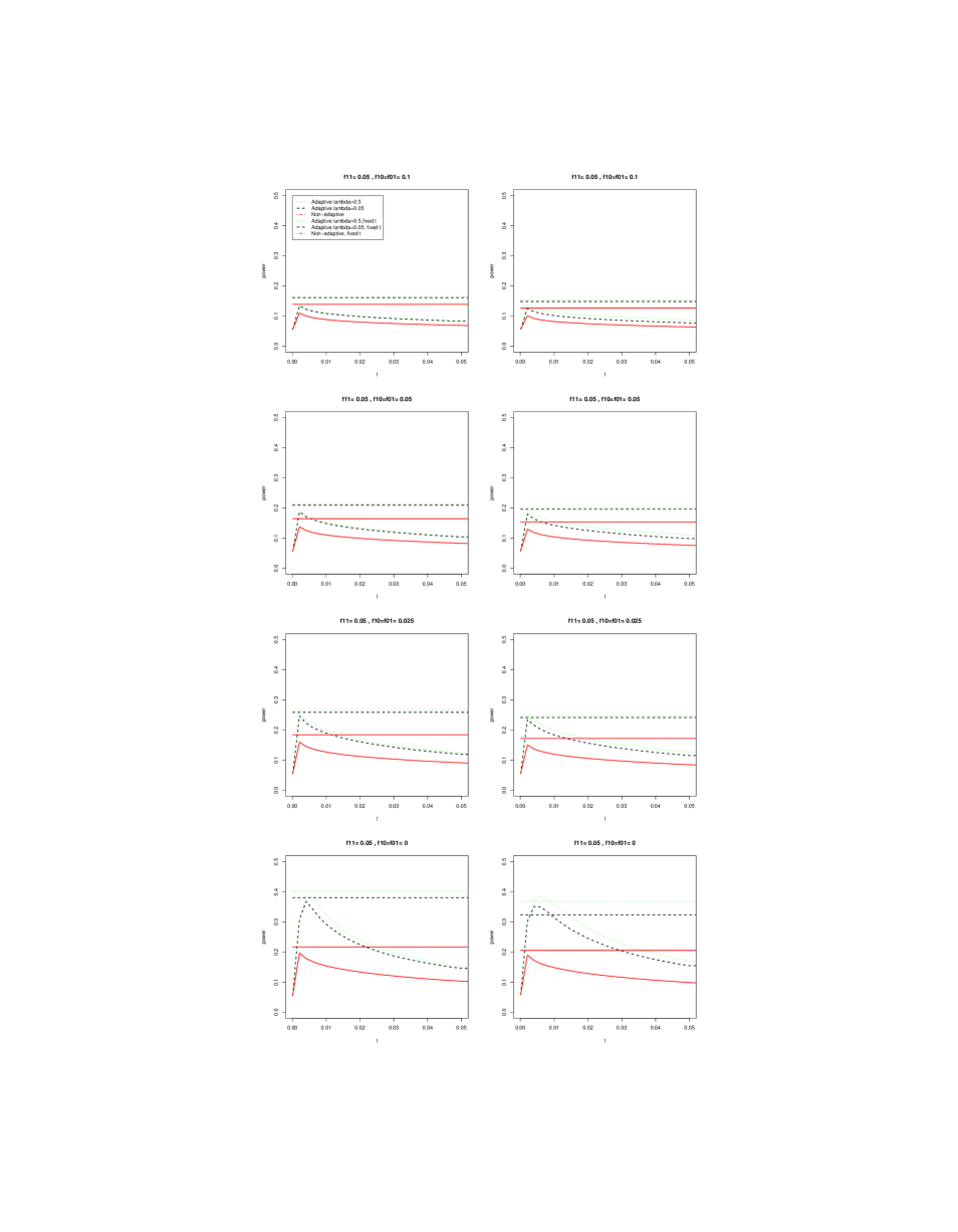
Figure 1: Column 1: Independence setting; Columns 2: Equicorrelation with $\rho=0.25$. The power versus fixed threshold $t$ is shown for $\mu=3$ for the adaptive-Bonferroni-replicability procedure (dashed black with $\lambda=0.05$ and dotted green with $\lambda=0.5$) and non-adaptive Bonferroni-replicability procedure (solid red), along with the power of these procedures with data-dependent thresholds. In all settings $m=1000$, $\alpha=0.05,\alpha_{1}=0.025$.

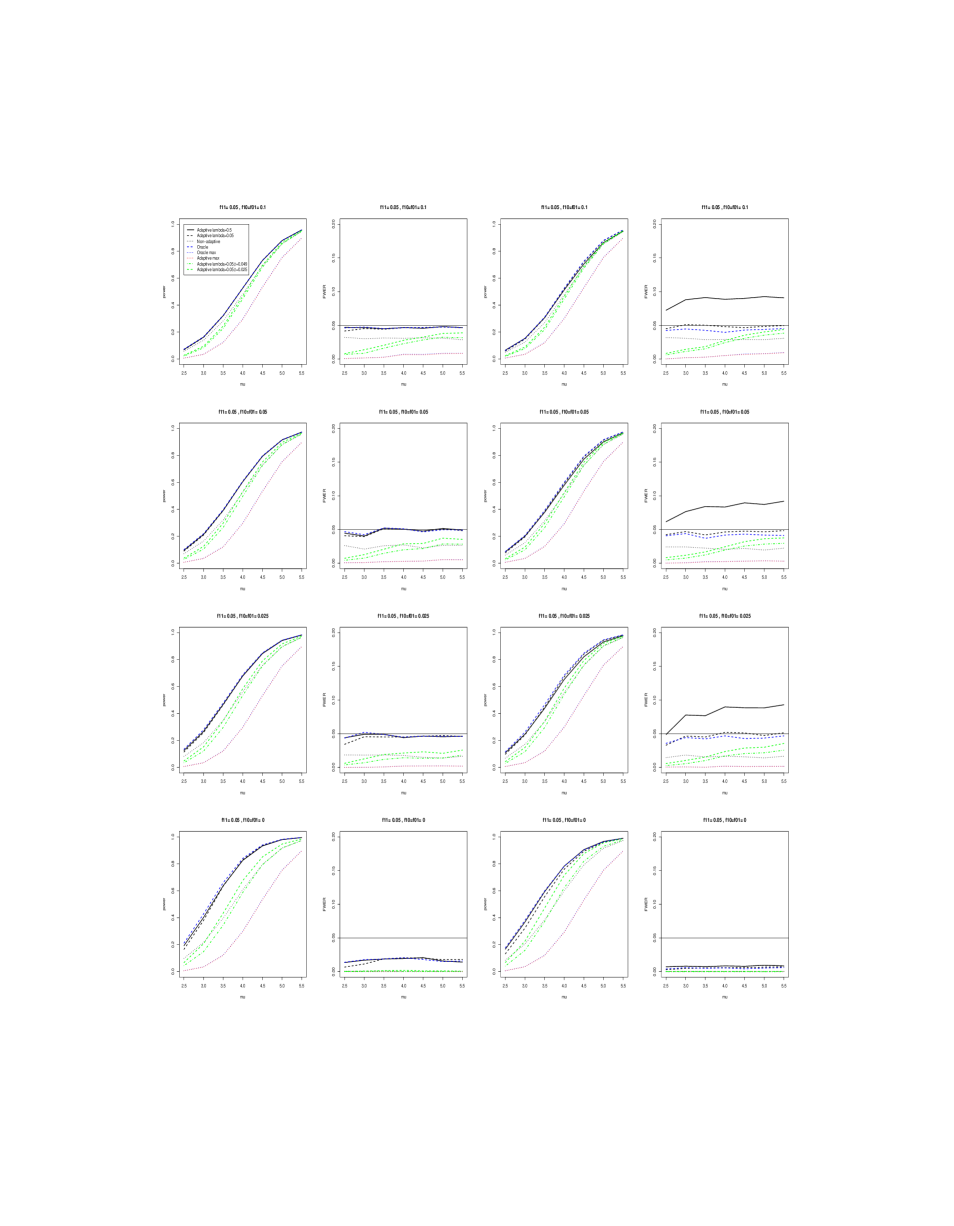
Figure 2: Columns 1 and 2: Independence setting; Columns 3 and 4: Equi-correlation with $\rho=0.25$. Power and FWER versus $\mu$ for the adaptive-Bonferroni-replicability procedure with data-dependent $(t_{1},t_{2})$ with $\lambda=0.5$ (solid black ) and with $\lambda=0.05$ (dashed black); Bonferroni-replicability procedure with data-dependent $(t_{1},t_{2})$ (dotted black); the oracle that knows which hypotheses are null in one study among the selected from the other study (dashed blue); oracle Max (dotted blue) and Max (dotted red); adaptive-Bonferroni-replicability with fixed $\lambda=0.05$ and fixed $t_{1}=t_{2}=0.049$ (dash-dot green) and fixed $t_{1}=t_{2}=0.025$ (dash green). In all settings $m=1000$, $\alpha=0.05,\alpha_{1}=0.025$.

7.2 Results for FDR controlling procedures

We considered the following novel procedures for replicability analysis with $\alpha=0.05,\alpha_{1}=0.025$: Non-adaptive-FDR-replicability with fixed or data-dependent $(t_{1},t_{2})$; adaptive-FDR-replicability with $\lambda\in\{0.05,0.5\}$ and fixed or data-dependent $(t_{1},t_{2})$.

Heller and Yekutieli, (2014) introduced the oracle Bayes procedure (oracleBayes), and showed that it has the largest rejection region while controlling the Bayes FDR. When $m$ is large and the data is generated from the mixture model, the Bayes FDR coincides with the frequentist FDR, so oracle Bayes is optimal for FDR control. We considered this oracle procedure for comparison with our novel procedures. The difference in power between the oracle Bayes and the novel frequentist procedures shows how much worse our procedures, which make no mixture-model assumptions, are from the (best yet unknown in practice) oracle procedure, which assumes the mixture model and needs as input its parameters. In addition, the following three procedures were considered: the empirical Bayes procedure (eBayes), as implemented in the R package repfdr (Heller et al., 2014b, ), which estimates the Bayes FDR and rejects the features with estimated Bayes FDR below $\alpha$, see Heller and Yekutieli, (2014) for details; the oracle BH on $\{\max(p_{1i},p_{2i}):i=1,\ldots,m\}$ (oracleMax); and the adaptive BH on $\{\max(p_{1i},p_{2i}):i=1,\ldots,m\}$ (adaptiveMax). Specifics about oracleMax and adaptiveMax follow. Applying the BH on $\{\max(p_{1i},p_{2i}):i=1,\ldots,m\}$ at level $x$, it is easy to show that the FDR level for independent features is at most $f_{00}x^{2}+(1-f_{00}-f_{11})x$. Therefore, the oracleMax procedure uses level $x$, which is the solution to $f_{00}x^{2}+(1-f_{00}-f_{11})x=0.05$, and the adaptiveMax procedure uses level $x$, which is the solution to $\hat{f}_{00}x^{2}+(1-\hat{f}_{00}-\hat{f}_{11})x=0.05$, where $\hat{f}_{00}$ and $\hat{f}_{11}$ are the estimated mixture fractions computed using the R package repfdr.

Figure 3 shows the power of novel procedures for various fixed selection thresholds $t_{1}=t_{2}=t$, as well as for the variants with data-dependent thresholds. There is a clear gain from adaptivity since the power curves for the adaptive procedures are above those for the non-adaptive procedures, for the same fixed threshold $t$. The choice of $t$ matters, and the choice $t=0.025$ is better than the choice $t=0.05$, and fairly close to the best $t$. We see that the power of the non-adaptive procedures with data-dependent selection thresholds is superior to the power of non-adaptive procedures with fixed thresholds. The same is true for the adaptive procedures in all the settings except for the last two rows of the equi-correlation setting, where the power of the adaptive procedures with data-dependent thresholds is slightly lower than the highest power for fixed thresholds $t_{1}=t_{2}=t.$ In these settings the number of selected hypotheses is on average lower than in other settings, and the fractions of true null hypotheses in one study among the selected in the other study are expected to be small. As a result, the solutions to the two non-linear equations solved using the estimates of the fractions of nulls are far from optimal. Therefore, when there is dependence within each study, and the number of selected hypotheses is small (say less than 100 per study), we suggest using the novel adaptive procedures with $t_{1}=t_{2}=\alpha/2$ instead of using data-dependent $(t_{1},t_{2})$.

Figure 4 shows the power and FDR versus $\mu$ under independence (columns 1 and 2) and under equi-correlation of the test statistics with $\rho=0.25$ (columns 3 and 4). The novel procedures are clearly superior to the competitors: the empirical Bayes procedure does not control the FDR when $m=1000$, and the actual level reaches above 0.1 under dependence; the oracleMax and adaptiveMax procedures have the lowest power in almost all settings. The novel adaptive procedures approach the power of the oracle Bayes as $f_{10}=f_{01}$ increase. The adaptive procedures with $\lambda=0.05$ and $\lambda=0.5$ have similar power, but the FDR with $\lambda=0.05$ is controlled in all dependence settings and the FDR with $\lambda=0.5$ is above the nominal level in three of the dependence settings. Our results concur with the results of Blanchard and Roquain, (2009) for single studies, that the preferred parameter is $\lambda=0.05$. We thus recommend the adaptive FDR-replicability procedure with $\lambda=\alpha$, for FDR control at level $\alpha$. We also recommend using data-dependent $(t_{1},t_{2})$, unless the test statistics are dependent within each study and the number of selected hypotheses from each study is expected to be small.

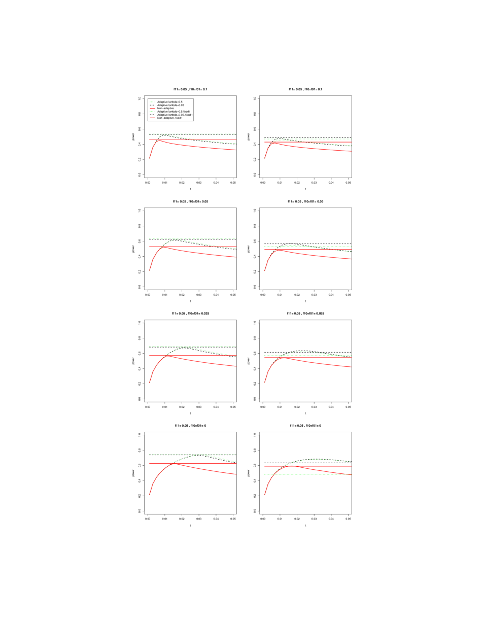
Figure 3: Column 1: Independence setting; Columns 2: Equi-correlation with $\rho=0.25$. The power versus fixed threshold $t$ is shown for $\mu=3$ for the adaptive and non-adaptive FDR-replicability procedures, along with the power of these procedures with data-dependent thresholds. In all settings $m=1000$, $\alpha=0.05,\alpha_{1}=0.025$.

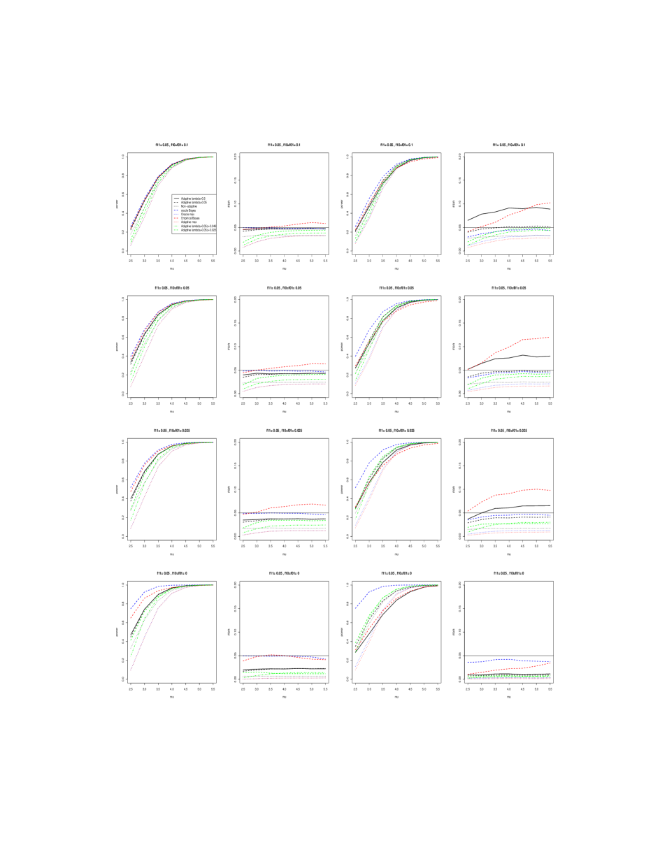
Figure 4: Columns 1 and 2: Independence setting; Columns 3 and 4: Equi-correlation with $\rho=0.25$. Power and FDR versus $\mu$ for the adaptive-FDR-replicability procedure with data-dependent $(t_{1},t_{2})$ with $\lambda=0.5$ (solid black) and with $\lambda=0.05$ (dashed black); Non-adaptive-FDR-replicability procedure with data-dependent $(t_{1},t_{2})$ (dotted black); the oracle Bayes (dashed blue) and empirical Bayes (dashed red); the oracle and adaptive BH on maximum $p$-value, (dotted blue and dotted red); adaptive-FDR-replicability procedure with $\lambda=0.05$ and fixed $t_{1}=t_{2}=0.049$ (dash-dot green) and fixed $t_{1}=t_{2}=0.025$ (dash green). In all settings $m=1000$, $\alpha=0.05,\alpha_{1}=0.025$.

8 Examples

8.1 Laboratory mice studies comparing behaviour across strains

It is well documented that in different laboratories, the comparison of behaviors of the same two strains may lead to opposite conclusions that are both statistically significant (Crabbe et al., (1999), Kafkafi et al., (2005), and Chapter 4 in Crusio et al., (2013)). An explanation may be the different laboratory environment (i.e. personnel, equipment, measurement techniques) affecting differently the study strains (i.e. an interaction of strain with laboratory). Richter et al., (2011) examined 29 behavioral measures from five commonly used behavioral tests (the barrier test, the vertical pole test, the elevated zero maze, the open field test, and the novel object test) on female mice from different strains in different laboratories with standardized conditions. Table 1 shows the one-sided $p$-value in the direction favored by the data based on the comparison of two strains in two laboratories, for each of the 29 outcomes.

Table 1: For 16 female mice from each of two inbred strains, ” C57BL6NCrl” and ”DBA/2NCrl”, in each of two laboratories, the Wilcoxon rank sum test one-sided $p$-value was computed for the test of no association between strain and behavioral endpoint. We show the $p$-values for the lab of H. Wurbel at the University of Giessen in column 3, and for the lab of P. Gass at the Central Institute of Mental Health, Mannheim in column 4. The direction of the alternative favored by the data is shown in column 2, and it is marked as ”X” if the laboratories differ in the direction of smallest one-sided $p$-value. The rows are the outcomes from 5 behavioural tests: the barrier test (row 1); the vertical pole test (row 2); the elevated zero maze (rows 3-11) ; the open field test (rows 12-19); the novel object test (rows 20-29).

$\min(P_{ij}^{L},P_{ij}^{R})$ Alternative $i=1$ $i=2$ 1 X 0.3161 0.0218 2 $C57BL<DBA$ 0.0012 0.0000 3 X 0.0194 0.1120 4 $C57BL<DBA$ 0.0095 0.2948 5 $C57BL<DBA$ 0.1326 0.0028 6 $C57BL>DBA$ 0.1488 0.0003 7 $C57BL>DBA$ 0.2248 0.0000 8 X 0.4519 0.0005 9 $C57BL<DBA$ 0.0061 0.0000 10 $C57BL<DBA$ 0.0071 0.0888 11 X 0.4297 0.1602 12 $C57BL<DBA$ 0.0918 0.0506 13 X 0.0918 0.0001 14 $C57BL<DBA$ 0.0000 0.0048 15 X 0.0005 0.0550

$\min(P_{ij}^{L},P_{ij}^{R})$ Alternative $i=1$ $i=2$ 16 $C57BL<DBA$ 0.0059 0.0002 17 $C57BL>DBA$ 0.0176 0.0003 18 X 0.0000 0.0538 19 $C57BL<DBA$ 0.0000 0.1727 20 $C57BL<DBA$ 0.0157 0.0001 21 $C57BL<DBA$ 0.0000 0.0234 22 $C57BL<DBA$ 0.3620 0.0176 23 $C57BL<DBA$ 0.0000 0.0001 24 $C57BL<DBA$ 0.0000 0.0076 25 $C57BL<DBA$ 0.0000 0.0000 26 $C57BL<DBA$ 0.0000 0.0003 27 $C57BL<DBA$ 0.0000 0.0001 28 $C57BL<DBA$ 0.0000 0.0550 29 X 0.0033 0.3760

The example is too small for considering the empirical Bayes approach. The approach suggested in Benjamini et al., (2009) of using for each feature the maximum of the two studies $p$-values, i.e., $2\min\{\max(p_{1j}^{L},p_{2j}^{L}),\max(p_{1j}^{R},p_{2j}^{R})\}$, detected overall fewer outcomes than using our novel procedures both for FWER and for FDR control.

Table 2 shows the FWER/FDR non-adaptive and adaptive $r$-values, for the selected features, according to the rule which selects all features with two-sided $p$-values that are at most 0.05. We did not consider data-dependent thresholds since the number of features examined was only 29, which could result in highly variable data-dependent thresholds and a power loss comparing to procedures with fixed thresholds, as was observed in simulations. At the $\alpha=0.05$ level, for FWER control, four discoveries were made by using Bonferroni on the maximum $p$-values, and five discoveries were made with the non-adaptive and adaptive Bonferroni-replicability procedures. At the $\alpha=0.05$ level, for FDR control, nine discoveries were made by using BH on the maximum $p$-values, and nine and twelve discoveries were made with the non-adaptive FDR and adaptive FDR-replicability procedures, respectively. Note that the adaptive $r$-values can be less than half the non-adaptive $r$-values, since $\hat{\pi}_{0}^{{I}}=0.44$ and $\hat{\pi}_{0}^{{II}}=0.47$.

Table 2: The replicability analysis results for the data in Table 1, after selection of features with two-sided $p$-values at most 0.05 (i.e. $t_{1}=t_{2}=0.025$). Only the twelve features in $\mathcal{S}_{1}\cap\mathcal{S}_{2}$ are shown, where $S_{1}=20$, $S_{2}=19$. For each selected feature, we show the $r$-values based on Bonferroni (column 5), FDR (column 6), adaptive Bonferroni (column 7), and the adaptive FDR (column 8). The adaptive procedures used $\lambda=0.05$.

index		$\min(P_{ij}^{L},P_{ij}^{R})$		Non-adaptive		Adaptive
selected	Alternative	$i=1$	$i=2$	Bonf	FDR	Bonf	FDR
2	$C57BL<DBA$	0.0012	0.0000	0.0452	0.0090	0.0200	0.0040
9	$C57BL<DBA$	0.0061	0.0000	0.2323	0.0290	0.1029	0.0129
14	$C57BL<DBA$	0.0000	0.0048	0.1910	0.0290	0.0905	0.0129
16	$C57BL<DBA$	0.0059	0.0002	0.2237	0.0290	0.0992	0.0129
17	$C57BL>DBA$	0.0176	0.0003	0.6679	0.0607	0.2960	0.0269
20	$C57BL<DBA$	0.0157	0.0001	0.5974	0.0597	0.2648	0.0265
21	$C57BL<DBA$	0.0000	0.0234	0.9363	0.0780	0.4435	0.0370
23	$C57BL<DBA$	0.0000	0.0001	0.0022	0.0011	0.0010	0.0005
24	$C57BL<DBA$	0.0000	0.0076	0.3037	0.0337	0.1439	0.0160
25	$C57BL<DBA$	0.0000	0.0000	0.0005	0.0005	0.0003	0.0003
26	$C57BL<DBA$	0.0000	0.0003	0.0126	0.0032	0.0060	0.0015
27	$C57BL<DBA$	0.0000	0.0001	0.0038	0.0013	0.0018	0.0006

8.2 Microarray studies comparing groups with different cancer severity

Freije et al., (2004) and Phillips et al., (2004) compared independently the expression levels in patients with grade $III$ and grade $IV$ brain cancer. Both studies used the Affymetrix HG U133 oligonucleotide arrays, with 22283 probes in each study. The study of Freije et al., (2004) (GEO accession GSE4412) included 26 subjects with tumors diagnosed as grade III glioma and 59 subjects with tumor diagnosis of grade IV glioma, all undergoing surgical treatment at the university of California, Los Angeles. The study of Phillips et al., (2004) (GEO accession GSE4271) included 24 grade III subjects, and 76 grade IV subjects, from the M.D. Anderson Cancer Center (MDA). The Wilcoxon rank sum test $p$-values were computed for each probe in each study in order to quantify the evidence against no association of probe measurement with tumor subgroup.

We used the R package repfdr (Heller et al., 2014b, ) to get the following estimated fractions, among the 22283 probes: 0.39 with $\vec{h}=(0,0)$; 0.16 with $\vec{h}=(1,1)$; 0.13 with $\vec{h}=(-1,-1)$; 0.10 with $\vec{h}=(0,1)$; 0.08 with $\vec{h}=(-1,0)$; 0.07 with $\vec{h}=(0,-1)$; 0.07 with $\vec{h}=(1,0)$; 0.00 with $\vec{h}=(-1,1)$ or $\vec{h}=(1,-1)$.

For FWER-replicability, the recommended Procedure 4.1 with $\lambda=0.05$ and data-dependent thresholds $t_{1}=6.5*10^{-5},t_{2}=5.1*10^{-5}$ discovered 340 probes. For comparison, the non-adaptive and adaptive Bonferroni-replicability procedure with fixed thresholds $t_{1}=t_{2}=0.025$ discovered only 90 and 124 probes, respectively. The Bonferroni on maximum $p$-values discovered only 47 probes.

For FDR-replicability, the recommended adaptive procedure in Section 4 with $\lambda=0.05$ and data-dependent thresholds $t_{1}=0.021,t_{2}=0.024$ discovered 3383 probes. For comparison, the non-adaptive and adaptive FDR-replicability procedure with fixed selection thresholds $t_{1}=t_{2}=0.025$ discovered 2288 and 3299 probes, respectively. The adaptive $r$-values can be half the non-adaptive $r$-values, since $\hat{\pi}_{0}^{I}=0.51$ and $\hat{\pi}_{0}^{II}=0.49$. Among the two competing approaches, the BH on maximum $p$-values discovered only 1238 probes, and the empirical Bayes procedure discovered 4320 probes. Among the 3383 probes discovered by our approach, 3377 were also discovered by the empirical Bayes procedure.

9 Discussion

In this paper we proposed novel procedures for establishing replicability in two studies. First, we introduced procedures that take the selected set of features in each of two studies, and infer about the replicability of features selected in both studies while controlling for false replicability claims. We proved that the FWER controlling procedure is valid (i.e., controls the error rate at the desired nominal level) for any dependence within each study, and that the FDR controlling procedure is valid under independence of the test statistics within each study, and suggested also a more conservative procedure that is valid for arbitrary dependence. Next, we suggested incorporating the plug-in estimates of the fraction of nulls in one study among the selected features by the other study, which can be estimated as long as the $p$-values for the union of features selected is available. We proved that the resulting adaptive FWER and FDR controlling procedures are valid under independence of the test statistics within each study. Our empirical investigations showed that the adaptive procedures remain valid even when the independence assumption is violated, as long as we use $\lambda=\alpha$ as a parameter for the plug-in estimates, as suggested by Blanchard and Roquain, (2009) for the adaptive BH procedure. Finally, when two full studies are available that examine the same features, we suggested selecting features for replicability analysis that have $p$-values below certain thresholds. We showed that selecting the features with one-sided $p$-values below $\alpha/2$ has good power, but that the power can further be improved if we use data-dependent thresholds, which receive the values that will lead to the procedure selecting exactly the features that are discovered as having replicated findings.

Our practical guidelines for establishing replicability are to use the adaptive procedure for the desired error rate control, with $\lambda=\alpha$. Moreover, based on the simulation results we suggest using the data-dependent selection thresholds when two full studies are available if the number of selected features in each study is expected to be large enough (say above 100), and using the fixed thresholds $t_{1}=t_{2}=\alpha/2$ otherwise. We would like to note that the $r$-value computation is more involved when the thresholds are data-dependent, since these thresholds depend on the nominal level $\alpha$. An interesting open question is how to account for multiple solutions of the two non-linear equations that are solved in order to find the data-dependent thresholds.

The suggested procedures can be generalized to the case that more than two studies are available. It is possible to either aggregate multiple results of pairwise replicability analyses, or to first aggregate the data and then apply a single replicability analysis on two meta-analysis $p$-values. The aim of the replicability analysis may also be redefined to be that of discovering features that have replicated findings in at least $u$ studies, where $u$ can range from two to the total number of studies. Other extensions include weighting the features differently, as suggested by Genovese et al., (2006), based on prior knowledge on the features, and replicability analysis on multiple families of hypotheses while controlling more general error rates, as suggested by Benjamini and Bogomolov, (2013).

Appendix A Notation for technical derivations

For the technical derivations, the following notation will be used. Let $p_{i}$ be the $m$-dimensional vector of $p$-values for study $i,$ $\mathcal{S}_{i}(p_{i})$ be the index set of features selected from study $i$ based on the vector of $p$-values $p_{i},$ and $S_{i}(p_{i})$ be the cardinality of this set, for $i\in\{1,2\}.$ Let $P_{i}^{(j)}=(P_{i1},\ldots,P_{i,j-1},P_{i,j+1},\ldots,P_{im})$ be the vector of $p$-values for the $m-1$ features excluding $j$, for $i=1,2$. When the selection rule by which the set $\mathcal{S}_{i}$ is selected is stable, define $\mathcal{S}_{i}^{(j)}\subseteq\{1,\ldots,j-1,j+1,\ldots,m\}$ as the set of indices selected along with $j,$ if $j\in\mathcal{S}_{i},$ and $\mathcal{S}_{i,\lambda}^{(j)}$ as $\mathcal{S}_{i}^{(j)}\cap\{l\neq j:P_{il}\leq\lambda\}$ if $j\in\mathcal{S}_{i,\lambda},$ for $i\in\{1,2\},$ and let $S_{i}^{(j)}=|\mathcal{S}_{i}^{(j)}|$. Define $\mathcal{S}_{i}^{(j)}(t_{i})=\{l:p_{il}\leq t_{i},l\neq j\}$ as the index set of features with $p$-value at most $t_{i}$ from the vector of $p$-values $p_{i}^{(j)}$, and let $S_{i}^{(j)}(t_{i})=|\mathcal{S}_{i}^{(j)}(t_{i})|$. For $c\in(0,1),$ we write $\alpha_{1}=c\alpha$ and $\alpha_{2}=\alpha-\alpha_{1}.$

Appendix B Proof of Theorems 3.2 and 4.2

In the proofs of Theorems 3.2 and 4.2 we use the following lemma. The lemma is proven in the end of the section.

Lemma B.1.

Let $\mathcal{S}_{i}$ be the selected set of features based on study $i$, for $i=1,2$. Let $r_{j},\,\,j\in\mathcal{S}_{1}\cap\mathcal{S}_{2}$ be the Bonferroni-type $r$-values:

$$r_{j}=\max\left\{\frac{W_{1}p_{1j}}{c},\frac{W_{2}p_{2j}}{1-c}\right\},\,\,j\in\mathcal{S}_{1}\cap\mathcal{S}_{2},$$ (B.1)

where $c\in(0,1)$ is a constant and $W_{1},W_{2}$ may be constants or random variables based on $p$-values. The FDR $r$-values based on the Bonferroni-type $r$-values are:

$$r^{FDR}_{j}=\min_{\{i:\,r_{i}\geq r_{j},i\in\mathcal{S}_{1}\cap\mathcal{S}_{2}\}}\frac{r_{i}}{rank(r_{i})},\,\,j\in\mathcal{S}_{1}\cap\mathcal{S}_{2},$$

where $rank(r_{i})$ is the rank of the Bonferroni-type $r$-value for feature $i\in\mathcal{S}_{1}\cap\mathcal{S}_{2}$, with maximum rank for ties.

1. The procedure that declares as replicated the features with FDR r-values at most $\alpha$ is equivalent to the following procedure on the selected features $\mathcal{S}_{1}\cap\mathcal{S}_{2}$:

   1. Let

      $$R\triangleq\max\left\{r:\sum_{j\in\mathcal{S}_{1}\cap\mathcal{S}_{2}}\textbf{I}\left[(p_{1j},p_{2j})\leq\left(\frac{r\alpha_{1}}{W_{1}},\frac{r\alpha_{2}}{W_{2}}\right)\right]=r\right\}.$$

   2. The set of indices with replicability claims is

      $$\mathcal{R}=\{j:(p_{1j},p_{2j})\leq\left(\frac{R\alpha_{1}}{W_{1}},\frac{R\alpha_{2}}{W_{2}}\right),\,\,j\in\mathcal{S}_{1}\cap\mathcal{S}_{2}\}.$$

2. The procedure that declares as replicated the features with FDR r-values at most $\alpha$ controls the FDR for replicability analysis at level $\alpha$ if the following conditions are satisfied:

   1. The $p$-values corresponding to true null hypotheses are each independent of all the other $p$-values.

   2. For each $j\in\{1,\ldots,m\},$ there exist random variables (or constants) $W_{1}^{(j)},W_{2}^{(j)}$ defined on the space $(P_{1}^{(j)},P_{2}^{(j)})$ such that if $j\in\mathcal{S}_{1}\cap\mathcal{S}_{2},$ then $W_{1}=W_{1}^{(j)},$ $W_{2}=W_{2}^{(j)},$and for arbitrary fixed vectors $p_{1}$and $p_{2}$ it holds:

      $$\textbf{I}[j\in\mathcal{S}_{2}(p_{2})]E(1/W_{1}^{(j)}\,|\,P_{2}=p_{2})\leq\frac{1}{\sum_{j\in\mathcal{S}_{2}(p_{2})}(1-H_{1j})}$$ (B.2)

      $$\textbf{I}[j\in\mathcal{S}_{1}(p_{1})]E(1/W_{2}^{(j)}\,|\,P_{1}=p_{1})\leq\frac{1}{\sum_{j\in\mathcal{S}_{1}(p_{1})}(1-H_{2j})}.$$ (B.3)

Proof of item 1 of Theorem 3.2 The result of item 1 of Theorem 3.2 follows from Lemma B.1. The conditions of Lemma B.1 hold with $W_{1}=S_{2},$ $W_{1}^{(j)}=1+S_{2}^{(j)},$ and $W_{2}=S_{1},$ $W_{2}^{(j)}=1+S_{1}^{(j)}.$ In order to see it, note that for $j\in\mathcal{S}_{1}\cap\mathcal{S}_{2},$ $S_{i}=1+S_{i}^{(j)}$ for $i\in\{1,2\}.$ In addition, note that for arbitrary fixed vector $p_{2}$ and $j\in\{1,\ldots,m\}$

$$\textbf{I}[j\in\mathcal{S}_{2}(p_{2})]E\left(\frac{1}{W_{1}^{(j)}}\,|\,P_{2}=p_{2}\right)= \textbf{I}[j\in\mathcal{S}_{2}(p_{2})]E\left(\frac{1}{1+S_{2}^{(j)}}\,|P_{2}=p_{2}\right)$$

$$= \textbf{I}[j\in\mathcal{S}_{2}(p_{2})]\left(\frac{1}{S_{2}(p_{2})}\,\right)\leq\frac{1}{\sum_{j\in\mathcal{S}_{2}(p_{2})}(1-H_{1j})}.$$

Thus we have proved inequality (B.2). The proof of inequality (B.3) is similar.

Proof of Theorem 4.2 The result of Theorem 4.2 follows from Lemma B.1. The conditions of Lemma B.1 hold with $\mathcal{S}_{i,\lambda},i=1,2$ as the selected sets, and

$$W_{1}=S_{2,\lambda}\hat{\pi}_{0}^{{I}}=\frac{1+\sum_{i\in\mathcal{S}_{2,\lambda}}\textbf{I}(P_{1i}>\lambda)}{(1-\lambda)},\,\,W_{1}^{(j)}=\frac{1+\sum_{i\in\mathcal{S}_{2,\lambda,i\neq j}}\textbf{I}(P_{1i}>\lambda)}{(1-\lambda)},$$

$$W_{2}=S_{1,\lambda}\hat{\pi}_{0}^{{II}}=\frac{1+\sum_{i\in\mathcal{S}_{1,\lambda}}\textbf{I}(P_{2i}>\lambda)}{(1-\lambda)},\,\,W_{2}^{(j)}=\frac{1+\sum_{i\in\mathcal{S}_{1,\lambda,i\neq j}}\textbf{I}(P_{2i}>\lambda)}{(1-\lambda)}.$$

In order to see it, note that if $j\in\mathcal{S}_{1,\lambda}\cap\mathcal{S}_{2,\lambda},$ it holds that $\max\{P_{1j},P_{2j}\}\leq\lambda.$ In addition, it was shown in the proof of Theorem 4.1 that for arbitrary fixed vector $p_{2}$ and $j\in\{1,\ldots,m\}$

$$\textbf{I}[j\in\mathcal{S}_{2,\lambda}(p_{2})]E\left(\frac{1}{W_{1}^{(j)}}\,|\,P_{2}=p_{2}\right)\leq$$

$$\textbf{I}[j\in\mathcal{S}_{2,\lambda}(p_{2})]E\left(1/\left(\frac{1+\sum_{i\in\mathcal{S}_{2,\lambda,i\neq j}}(1-H_{1j})\textbf{I}(P_{1i}>\lambda)}{1-\lambda}\right)\,|\,P_{2}=p_{2}\right)\leq$$

$$\frac{1}{\sum_{j\in\mathcal{S}_{2,\lambda}(p_{2})}(1-H_{1j})}.$$

The proof of inequality (B.3) is similar.
Proof of item 1 of Lemma B.1. Note that the procedure given in item 1 of Lemma B.1 can be written as follows:

1. Let

   $$R=\max\left\{r:\sum_{j\in\mathcal{S}_{1}\cap\mathcal{S}_{2}}\textbf{I}\left[r_{j}\leq r\alpha\right]=r\right\}.$$

2. The set of indices with replicability claims is

   $$\mathcal{R}=\{j:r_{j}\leq R\alpha,\,\,j\in\mathcal{S}_{1}\cap\mathcal{S}_{2}\}.$$

Let $r_{0}=\max\left\{r:\sum_{j\in\mathcal{S}_{1}\cap\mathcal{S}_{2}}\textbf{I}\left[r_{j}\leq r\alpha\right]\geq r\right\}.$ We prove that $R=r_{0}$ by contradiction. From the definitions of $r_{0}$ and $R$ it follows that if $R\neq r_{0},$ then $r_{0}>R,$ and $\sum_{j\in\mathcal{S}_{1}\cap\mathcal{S}_{2}}\textbf{I}\left[r_{j}\leq r_{0}\alpha\right]\geq r_{0}+1.$ However, since $\sum_{j\in\mathcal{S}_{1}\cap\mathcal{S}_{2}}\textbf{I}\left[r_{j}\leq(r_{0}+1)\alpha\right]\geq\sum_{j\in\mathcal{S}_{1}\cap\mathcal{S}_{2}}\textbf{I}\left[r_{j}\leq r_{0}\alpha\right]$ it follows that $r_{0}+1$ is also in $\left\{r:\sum_{j\in\mathcal{S}_{1}\cap\mathcal{S}_{2}}\textbf{I}\left[r_{j}\leq r\alpha\right]\geq r\right\}$, thus contradicting the definition of $r_{0}$ as being the greatest value in this set. Thus we have proved that

$$R=\max\left\{r:\sum_{j\in\mathcal{S}_{1}\cap\mathcal{S}_{2}}\textbf{I}\left[r_{j}\leq r\alpha\right]\geq r\right\}.$$ (B.4)

We now prove that the procedure that declares as replicated the features with FDR r-values at most $\alpha$ is equivalent to the following procedure in item 1, i.e.

$$\{j:r_{j}^{FDR}\leq\alpha\}=\{j:r_{j}\leq R\alpha\},$$ (B.5)

where $R$ is given in (B.4). Let us first prove that

$$\{j:r_{j}^{FDR}\leq\alpha\}\subseteq\{j:r_{j}\leq R\alpha\}.$$ (B.6)

Let $j\in\{j:r_{j}^{FDR}\leq\alpha\}$ be arbitrary fixed. There exists $i_{0}\in\mathcal{S}_{1}\cap\mathcal{S}_{2}$ such that $r_{i_{0}}\geq r_{j}$ and

$$\frac{r_{i_{0}}}{rank(r_{i_{0}})}=\min_{\{i:\,r_{i}\geq r_{j},i\in\mathcal{S}_{1}\cap\mathcal{S}_{2}\}}\frac{r_{i}}{rank(r_{i})}\leq\alpha.$$

Thus $r_{i_{0}}\leq rank(r_{i_{0}})\alpha.$ Therefore, $rank(r_{i_{0}})\leq\sum_{j\in\mathcal{S}_{1}\cap\mathcal{S}_{2}}\textbf{I}\left[r_{j}\leq rank(r_{i_{0}})\alpha\right]$. This inequality and the expression for $R$ given in (B.4) yield that $rank(r_{i_{0}})\leq R.$ It follows that $r_{i_{0}}\leq R\alpha.$ Recall that $r_{j}\leq r_{i_{0}},$ therefore $r_{j}\leq R\alpha.$ Thus we have proved $(\ref{muhal1}).$ Let us now prove that

$$\{j:r_{j}\leq R\alpha\}\subseteq\{j:r_{j}^{FDR}\leq\alpha\}.$$ (B.7)

Let $j\in\mathcal{S}_{1}\cap\mathcal{S}_{2}$ be an arbitrary fixed index such that $r_{j}\leq R\alpha.$ Since $r_{j}\leq r_{(R)}$, and $\frac{r_{(R)}}{R}\leq\alpha$ (where $r_{(R)}$ is the $R$’th largest $r$-value), it follows that

$$r_{j}^{FDR}=\min_{\{i:\,r_{i}\geq r_{j},i\in S_{1}\cap S_{2}\}}\frac{r_{i}}{rank(r_{i})}\leq\alpha.$$

Thus we have proved (B.7), which completes the proof of (B.5) and of item 1.
Proof of item 2 of Lemma B.1 For $j\in\{1,\ldots,m\}$ let us define $C_{k}^{(j)}$ as the event in which if $r_{j}^{FDR}\leq\alpha,$ then the total number of FDR $r$-values which are at most $\alpha$ is $k.$ It follows from item 1 and from condition (ii) of item 2 that the event $C_{k}^{(j)}$ is defined on the space $(P_{1}^{(j)},P_{2}^{(j)})$ as follows. Let

$$T_{i}^{(j)}=\left\{\begin{array}[]{cl}\max\left(\frac{W_{1}^{(j)}p_{1i}}{c},\frac{W_{2}^{(j)}p_{2i}}{1-c}\right)&\text{if}\,\,i\in\mathcal{S}_{1}^{(j)}\cap\mathcal{S}_{2}^{(j)},\\ \infty&\text{otherwise. }\\ \end{array}\right.$$ (B.10)

and let $T^{(j)}_{1}\leq\ldots\leq T^{(j)}_{m-1}$ be the sorted $T$-values, where we set $T_{0}^{(j)}=0.$ Note that $T_{i}^{(j)}=r_{i}$ for $i\in\mathcal{S}_{1}^{(j)}\cap\mathcal{S}_{2}^{(j)}.$ It follows from the equivalent procedure given in item 1 of Lemma B.1 that

$$C_{k}^{(j)}=\{(P_{1}^{(j)},P_{2}^{(j)}):\,T^{(j)}_{(k-1)}\leq k\alpha,T^{(j)}_{(k)}>(k+1)\alpha,\ldots,T^{(j)}_{(m-1)}>m\alpha\}.$$ (B.11)

Note that given $P_{1}=p_{1},$ for $j\in\mathcal{S}_{1}(p_{1}),$ $C_{k}^{(j)}=\emptyset$ for $k>S_{1}(p_{1})$, since the number of finite $T^{(j)}_{i}$’s is smaller or equal to $S_{1}(p_{1})-1.$ Similarly, given $P_{2}=p_{2}$, for $j\in\mathcal{S}_{2}(p_{2}),$ $C_{k}^{(j)}=\emptyset$ for $k>S_{2}(p_{2})$. In addition, note that $C_{k}^{(j)}$ and $C_{k^{\prime}}^{(j)}$ are disjoint events for any $k\neq k^{\prime}$ and $\sum_{k=1}^{S_{1}(p_{1})}\textmd{Pr}(C_{k}^{(j)}|P_{1}=p_{1})=\sum_{k=1}^{S_{2}(p_{2})}\textmd{Pr}(C_{k}^{(j)}|P_{2}=p_{2})=1.$

The FDR for replicability analysis is

$$FDR =\sum_{j=1}^{m}(1-H_{1j}H_{2j})\sum_{k=1}^{m}\frac{1}{k}\textmd{Pr}\left(j\in\mathcal{S}_{1}\cap\mathcal{S}_{2},r_{j}^{FDR}\leq\alpha,C_{k}^{(j)}\right)$$

$$=\sum_{j=1}^{m}(1-H_{1j}H_{2j})\sum_{k=1}^{m}\frac{1}{k}\textmd{Pr}\left(j\in\mathcal{S}_{1}\cap\mathcal{S}_{2},r_{j}\leq k\alpha,C_{k}^{(j)}\right)$$ (B.12)

$$\leq\sum_{j=1}^{m}(1-H_{1j})\sum_{k=1}^{m}\frac{1}{k}\textmd{Pr}\left(j\in\mathcal{S}_{1}\cap\mathcal{S}_{2},r_{j}\leq k\alpha,C_{k}^{(j)}\right)$$ (B.13)

$$+\sum_{j=1}^{m}(1-H_{2j})\sum_{k=1}^{m}\frac{1}{k}\textmd{Pr}\left(j\in\mathcal{S}_{1}\cap\mathcal{S}_{2},r_{j}\leq k\alpha,C_{k}^{(j)}\right)$$ (B.14)

where the equality in (B.12) follows from item 1, and the inequality in (B.13) follows from the fact that $1-H_{1j}H_{2j}\leq 2-H_{1j}-H_{2j}$ for all $j\in\{1,\ldots,m\}.$ We prove that for $(p_{1},p_{2})$ arbitrary fixed, the following inequalities hold for conditional expectations.

$$\sum_{j=1}^{m}(1-H_{1j})\sum_{k=1}^{m}\frac{1}{k}\textmd{Pr}\left(j\in\mathcal{S}_{1}\cap\mathcal{S}_{2},r_{j}\leq k\alpha,C_{k}^{(j)}\,|\,P_{2}=p_{2}\right)\leq\alpha_{1},$$ (B.15)

$$\sum_{j=1}^{m}(1-H_{2j})\sum_{k=1}^{m}\frac{1}{k}\textmd{Pr}\left(j\in\mathcal{S}_{1}\cap\mathcal{S}_{2},r_{j}\leq k\alpha,C_{k}^{(j)}\,|\,P_{1}=p_{1}\right)\leq\alpha_{2}.$$ (B.16)

Note that since these inequalities hold for all $p_{1}$ and $p_{2},$ they yield that the upper bounds in (B.15) and (B.16) hold for expressions in (B.13) and (B.14) respectively, therefore FDR for replicability analysis is upper bounded by $\alpha_{1}+\alpha_{2}=\alpha.$ Thus it remains to prove inequalities (B.15) and (B.16). We now prove inequality (B.15).

$$\sum_{j=1}^{m}(1-H_{1j})\sum_{k=1}^{m}\frac{1}{k}\textmd{Pr}\left(j\in\mathcal{S}_{1}\cap\mathcal{S}_{2},r_{j}\leq k\alpha,C_{k}^{(j)}\,|\,P_{2}=p_{2}\right)=$$

$$\sum_{j\in\mathcal{S}_{2}(p_{2})}(1-H_{1j})\sum_{k=1}^{S_{2}(p_{2})}\frac{1}{k}\textmd{Pr}\left(j\in\mathcal{S}_{1},r_{j}\leq k\alpha,C_{k}^{(j)}\,|\,P_{2}=p_{2}\right)\leq$$ (B.17)

$$\sum_{j\in\mathcal{S}_{2}(p_{2})}(1-H_{1j})\sum_{k=1}^{S_{2}(p_{2})}\frac{1}{k}\textmd{Pr}\left(j\in\mathcal{S}_{1},P_{1j}\leq\frac{kc\alpha}{W_{1}^{(j)}},C_{k}^{(j)}\,|\,P_{2}=p_{2}\right)\leq$$ (B.18)

$$\alpha_{1}\sum_{j\in\mathcal{S}_{2}(p_{2})}(1-H_{1j})\sum_{k=1}^{S_{2}(p_{2})}E\left(\frac{1}{W_{1}^{(j)}}\textbf{I}\left[C_{k}^{(j)}\right]\,|\,P_{2}=p_{2}\right)=$$

$$\alpha_{1}\sum_{j\in\mathcal{S}_{2}(p_{2})}(1-H_{1j})E\left(\frac{1}{W_{1}^{(j)}}\sum_{k=1}^{S_{2}(p_{2})}\textbf{I}\left[C_{k}^{(j)}\right]\,|\,P_{2}=p_{2}\right)=$$ (B.19)

$$\alpha_{1}\sum_{j\in\mathcal{S}_{2}(p_{2})}(1-H_{1j})E\left(\frac{1}{W_{1}^{(j)}}\,|\,P_{2}=p_{2}\right)\leq$$ (B.20)

$$\alpha_{1}\sum_{j\in\mathcal{S}_{2}(p_{2})}(1-H_{1j})\left(\frac{1}{\sum_{j\in\mathcal{S}_{2}(p_{2})}(1-H_{1j})}\right)=\alpha_{1}.$$

The inequality in (B.17) follows from condition (ii) of item 2. The inequality in (B.18) follows from the fact that the distribution of $P_{1j}$ is uniform or stochastically larger than uniform and $P_{1j}$ with $H_{1j}=0$ is independent of all other $p$-values. The equality in (B.19) follows from the fact that given $P_{2}=p_{2},$ $\cup_{k=1}^{S_{2}(p_{2})}C_{k}^{(j)}$ is the whole sample space represented as a union of disjoint events (as discussed above), therefore $\sum_{k=1}^{S_{2}(p_{2})}\textbf{I}\left[C_{k}^{(j)}\right]=1.$ The inequality in (B.20) follows from condition (ii) of item 2, inequality (B.2). Thus we proved inequality (B.15). Inequality (B.16) is proved similarly.
Proof of item 2 in Theorem 3.2. The proof is similar to the proof of item 3 of Theorem S3.2 in the Supplementary Material of Bogomolov and Heller, (2013). We give it below for completeness. For $j,k\in\{1,\ldots,m\},$ we define $\tilde{C}_{k}^{(j)}$ as the event in which if $\tilde{r}_{j}^{FDR}\leq\alpha,$ then the total number of arbitrary-dependence FDR $r$-values which are at most $\alpha$ is $k.$ Similarly to the proof of item 2 of Lemma B.1 it can be shown that the event $\widetilde{C}_{k}^{(j)}$ is defined on the space of $(P_{1}^{(j)},P_{2}^{(j)})$ as in (B.11), where $T$-values are replaced by $\tilde{T}$- values which are defined as follows.

$$\tilde{T}_{i}^{(j)}=\left\{\begin{array}[]{cl}\max\left(\frac{(\sum_{k=1}^{S_{2}^{(j)}+1}1/k)(S_{2}^{(j)}+1)p_{1i}}{c},\frac{(\sum_{k=1}^{(S_{1}^{(j)}+1)}1/k)(S_{1}^{(j)}+1)p_{2i}}{1-c}\right)&\text{if}\,\,i\in\mathcal{S}_{1}^{(j)}\cap\mathcal{S}_{2}^{(j)},\\ \infty&\text{otherwise. }\\ \end{array}\right.$$ (B.23)

Note that $\tilde{T}_{i}^{(j)}=\tilde{r}_{i}$ for $i\in\mathcal{S}_{1}^{(j)}\cap\mathcal{S}_{2}^{(j)},$ where the expression for $\tilde{r}_{i}$ is given in (3.2). Similarly to the proof of item 2 of Lemma B.1, it can be shown that given $P_{1}=p_{1},$ $\tilde{C}_{k}^{(j)}=\emptyset$ for $j\in\mathcal{S}_{1}(p_{1})$ and $k>S_{1}(p_{1}),$ and $\cup_{k=1}^{S_{1}(p_{1})}\tilde{C}_{k}^{(j)}$ is the whole sample space. Given $P_{2}=p_{2},$ $\tilde{C}_{k}^{(j)}=\emptyset$ for $j\in\mathcal{S}_{2}(p_{2})$ and $k>S_{2}(p_{2}),$ and $\cup_{k=1}^{S_{2}(p_{2})}\tilde{C}_{k}^{(j)}$ is the whole sample space. In addition, $\tilde{C}_{k}^{(j)}$ and $\tilde{C}_{k^{\prime}}^{(j)}$ are disjoint events for any $k\neq k^{\prime}.$

We obtain the following inequality for the FDR for replicability analysis using derivations (B.12)-(B.14) where we replace $r_{j}^{FDR},$ $r_{j}$ and $C_{k}^{(j)}$ by $\tilde{r}_{j}^{FDR},$ $\tilde{r}_{j}$ and $\tilde{C}_{k}^{(j)},$ respectively.

$$FDR \leq\sum_{j=1}^{m}(1-H_{1j})\sum_{k=1}^{m}\frac{1}{k}\textmd{Pr}\left(j\in\mathcal{S}_{1}\cap\mathcal{S}_{2},\tilde{r}_{j}\leq k\alpha,\tilde{C}_{k}^{(j)}\right)$$

$$+\sum_{j=1}^{m}(1-H_{2j})\sum_{k=1}^{m}\frac{1}{k}\textmd{Pr}\left(j\in\mathcal{S}_{1}\cap\mathcal{S}_{2},\tilde{r}_{j}\leq k\alpha,\tilde{C}_{k}^{(j)}\right)$$ (B.24)

We now find an upper bound for the first term of the sum in (B.24). Let $p_{2}$ be arbitrary fixed. We define $\tilde{\alpha}_{1}=\alpha_{1}/(\sum_{i=1}^{S_{2}(p_{2})}1/i).$ We shall prove that

$$\sum_{j=1}^{m}(1-H_{1j})\sum_{k=1}^{m}\frac{1}{k}\textmd{Pr}\left(j\in\mathcal{S}_{1}\cap\mathcal{S}_{2},\tilde{r}_{j}\leq k\alpha,\tilde{C}_{k}^{(j)}\,|\,P_{2}=p_{2}\right)\leq\alpha_{1}.$$ (B.25)

Note that

$$\sum_{j=1}^{m}(1-H_{1j})\sum_{k=1}^{m}\frac{1}{k}\textmd{Pr}\left(j\in\mathcal{S}_{1}\cap\mathcal{S}_{2},\tilde{r}_{j}\leq k\alpha,\tilde{C}_{k}^{(j)}\,|\,P_{2}=p_{2}\right)=\sum_{j\in\mathcal{S}_{2}(p_{2})}(1-H_{1j})\times$$

$$\sum_{k=1}^{S_{2}(p_{2})}\frac{1}{k}\,\textmd{Pr}\left(S_{1}\left(\sum_{i=1}^{S_{1}}1/i\right)p_{2j}\leq k\alpha_{2},j\in\mathcal{S}_{1},P_{1j}\leq\frac{k\tilde{\alpha}_{1}}{S_{2}(p_{2})},\tilde{C}_{k}^{(j)}\,|\,P_{2}=p_{2}\right)$$

$$\leq\sum_{j\in\mathcal{S}_{2}(p_{2})}(1-H_{1j})\sum_{k=1}^{S_{2}(p_{2})}\frac{1}{k}\,\textmd{Pr}\left(P_{1j}\leq\frac{k\tilde{\alpha}_{1}}{S_{2}(p_{2})},\tilde{C}_{k}^{(j)}\,|\,P_{2}=p_{2}\right).$$

For each $j$ with ${H}_{1j}=0,$ $k\in\{1,\ldots,S_{2}(p_{2})\},$ and $l\in\{1,\ldots,k\},$ let us define:

$$p_{jkl}=\textmd{Pr}\left(P_{1j}\in\left(\frac{(l-1)\tilde{\alpha}_{1}}{S_{2}(p_{2})},\frac{l\tilde{\alpha}_{1}}{S_{2}(p_{2})}\right],\tilde{C}_{k}^{(j)}|P_{2}=p_{2}\right).$$

Note that for $j$ with ${H}_{1j}=0,$ $\textmd{Pr}\left(P_{1j}\leq x\right)\leq x$ for all $x\in[0,1]$, in particular $\textmd{Pr}\left(P_{1j}=0\right)=0.$ Therefore, for each $j$ with ${H}_{1j}=0$ and $k\in\{1,\ldots,S_{2}(p_{2})\},$

$$\textmd{Pr}\left(P_{1j}\leq\frac{k\tilde{\alpha}_{1}}{S_{2}(p_{2})},\tilde{C}_{k}^{(j)}\,|\,P_{2}=p_{2}\right)=\sum_{l=1}^{k}p_{jkl}.$$

Using this equality we obtain:

$$\sum_{j\in\mathcal{S}_{2}(p_{2})}(1-H_{1j})\sum_{k=1}^{S_{2}(p_{2})}\frac{1}{k}\textmd{Pr}\left(P_{1j}\leq\frac{k\tilde{\alpha}_{1}}{S_{2}(p_{2})},\,\tilde{C}_{k}^{(j)}\,|\,P_{2}=p_{2}\right)=$$

$$\sum_{j\in\mathcal{S}_{2}(p_{2})}(1-H_{1j})\sum_{k=1}^{S_{2}(p_{2})}\frac{1}{k}\sum_{l=1}^{k}p_{jkl}=\sum_{j\in\mathcal{S}_{2}(p_{2})}(1-H_{1j})\sum_{l=1}^{S_{2}(p_{2})}\sum_{k=l}^{S_{2}(p_{2})}\frac{1}{k}p_{jkl}\leq$$

$$\sum_{j\in\mathcal{S}_{2}(p_{2})}(1-H_{1j})\sum_{l=1}^{S_{2}(p_{2})}\sum_{k=l}^{S_{2}(p_{2})}\frac{1}{l}p_{jkl}\leq\sum_{j\in\mathcal{S}_{2}(p_{2})}(1-H_{1j})\sum_{l=1}^{S_{2}(p_{2})}\frac{1}{l}\sum_{k=1}^{S_{2}(p_{2})}p_{jkl}.$$ (B.26)

Since $\cup_{k=1}^{S_{2}(p_{2})}C_{k}^{(j)}$ is a union of disjoint events, we obtain for each $j$ with ${H}_{1j}=0$ and $l\in\{1,\ldots,S_{2}(p_{2})\}$:

$$\sum_{k=1}^{S_{2}(p_{2})}p_{jkl}=\textmd{Pr}\left(P_{1j}\in\left(\frac{(l-1)\tilde{\alpha}_{1}}{S_{2}(p_{2})},\frac{l\tilde{\alpha}_{1}}{S_{2}(p_{2})}\right],\,\cup_{k=1}^{S_{2}(p_{2})}\tilde{C}_{k}^{(j)}\,|\,P_{2}=p_{2}\right)$$

$$\leq\textmd{Pr}\left(P_{1j}\in\left(\frac{(l-1)\tilde{\alpha}_{1}}{S_{2}(p_{2})},\frac{l\tilde{\alpha}_{1}}{S_{2}(p_{2})}\right]\,|\,P_{2}=p_{2}\right)$$

$$=\textmd{Pr}\left(P_{1j}\leq\frac{l\tilde{\alpha}_{1}}{S_{2}(p_{2})}\,|P_{2}=p_{2}\right)-\textmd{Pr}\left(P_{1j}\leq\frac{(l-1)\tilde{\alpha}_{1}}{S_{2}(p_{2})}\,|\,P_{2}=p_{2}\right).$$

Therefore for each $j$ with $H_{1j}=0$ we obtain:

$$\sum_{l=1}^{S_{2}(p_{2})}\frac{1}{l}\sum_{k=1}^{S_{2}(p_{2})}p_{jkl}\leq\sum_{l=1}^{S_{2}(p_{2})}\frac{1}{l}\left[\textmd{Pr}\left(P_{1j}\leq\frac{l\tilde{\alpha}_{1}}{S_{2}(p_{2})}\,|\,P_{2}=p_{2}\right)-\textmd{Pr}\left(P_{1j}\leq\frac{(l-1)\tilde{\alpha}_{1}}{S_{2}(p_{2})}\,|\,P_{2}=p_{2}\right)\right]$$

$$=\sum_{l=1}^{S_{2}(p_{2})}\frac{1}{l}\textmd{Pr}\left(P_{1j}\leq\frac{l\tilde{\alpha}_{1}}{S_{2}(p_{2})}\,|\,P_{2}=p_{2}\right)-\sum_{l=0}^{S_{2}(p_{2})-1}\frac{1}{l+1}\textmd{Pr}\left(P_{1j}\leq\frac{l\tilde{\alpha}_{1}}{S_{2}(p_{2})}\,|\,P_{2}=p_{2}\right)$$

$$=\sum_{l=1}^{S_{2}(p_{2})-1}\left(\frac{1}{l}-\frac{1}{l+1}\right)\textmd{Pr}\left(P_{1j}\leq\frac{l\tilde{\alpha}_{1}}{S_{2}(p_{2})}\,|\,P_{2}=p_{2}\right)+\frac{1}{S_{2}(p_{2})}\textmd{Pr}\left(P_{1j}\leq\tilde{\alpha}_{1}\,|\,P_{2}=p_{2}\right)$$

$$\leq\sum_{l=1}^{S_{2}(p_{2})-1}\frac{1}{l+1}\left(\frac{\tilde{\alpha}_{1}}{S_{2}(p_{2})}\right)+\frac{\tilde{\alpha}_{1}}{S_{2}(p_{2})}=\left(\frac{\tilde{\alpha}_{1}}{S_{2}(p_{2})}\right)\sum_{l=1}^{S_{2}(p_{2})}\frac{1}{l}=\frac{\alpha_{1}}{S_{2}(p_{2})}.$$ (B.27)

The inequality in (B.27) follows from the null independence-across-studies condition and the fact that for $j$ with $H_{1j}=0,$ $\textmd{Pr}(P_{1j}\leq x)\leq x$ for all $x\in[0,1].$ Combining (B.26) with (B.27) we obtain the inequality in (B.25):

$$\sum_{j\in\mathcal{S}_{2}(p_{2})}(1-H_{1j})\sum_{k=1}^{S_{2}(p_{2})}\frac{1}{k}\textmd{Pr}\left(P_{1j}\leq\frac{k\tilde{\alpha_{1}}}{S_{2}(p_{2})},\,\tilde{C}_{k}^{(j)}\,|\,P_{2}=p_{2}\right)\leq\alpha_{1}\frac{\sum_{j\in\mathcal{S}_{2}(p_{2})}(1-H_{1j})}{S_{2}(p_{2})}\leq\alpha_{1}.$$

We have proved that the inequality in (B.25) holds for $p_{2}$ arbitrary fixed, therefore the first term of the sum in (B.24) is upper bounded by $\alpha_{1}.$ Similarly it can be proven that the second term of the sum in (B.24) is upper bounded by $\alpha_{2}.$ It follows from (B.24) that these two inequalities yield $FDR\leq\alpha_{1}+\alpha_{2}=\alpha.$

Appendix C Theoretical properties for Section 6

We use the following lemma to justify the empirical selection of $(t_{1},t_{2})$ for Procedure 3.1 based on Bonferroni.

Lemma C.1.

Assume that $G_{i}(t_{i}),i\in\{1,2\}$ are monotone increasing functions. Let $(t^{*}_{1},t^{*}_{2})$ be the solution to the following two equations:

$$t_{1}=\frac{\alpha_{1}}{G_{2}(t_{2})};\quad t_{2}=\frac{\alpha_{2}}{G_{1}(t_{1})}.$$ (C.1)

Then there does not exist a pair $(t_{1},t_{2})$ that dominates $(t_{1}^{*},t_{2}^{*})$ in the following sense:

$$\binom{\min\left(t_{1},\frac{\alpha_{1}}{G_{2}(t_{2})}\right)}{\min\left(\frac{\alpha_{2}}{G_{1}(t_{1})},t_{2}\right)}>\binom{\min\left(t_{1}^{*},\frac{\alpha_{1}}{G_{2}(t^{*}_{2})}\right)}{\min\left(\frac{\alpha_{2}}{G_{1}(t_{1}^{*})},t_{2}^{*}\right)},$$

where the strict inequality means that both coordinates are at least as large with $(t_{1},t_{2})$ as with $(t_{1}^{*},t_{2}^{*})$, but at least one coordinate is strictly larger.

See Appendix C.1 for a proof. Clearly, $S_{1}(t_{1})$ and $|\mathcal{S}_{1,\lambda}(t_{1})|\hat{\pi}_{0}^{{II}}$ are increasing functions of $t_{1}$, and similarly $S_{2}(t_{2})$ and $|\mathcal{S}_{2,\lambda}(t_{2})|\hat{\pi}_{0}^{{I}}$ are increasing functions of $t_{2}$. From Lemma C.1 it follows that the choice $(t^{*}_{1},t^{*}_{2})$ in equations (6.1) or (6.2) is not dominated by any other choice of $(t_{1},t_{2})$ in Procedure 3.2 and Procedure 4.1, respectively. Therefore, we suggest these data-dependent $(t^{*}_{1},t^{*}_{2})$.

Our next theorems state that the FWER and FDR of the non-adaptive procedures using the above data-dependent thresholds for selection are controlled under independence.

Theorem C.1.

If the $p$-values from true null hypotheses within each study are exchangeable, and each independent of all other $p$-values, then Procedure 3.1 based on Bonferroni with selection thresholds $(t_{1},t_{2})=(t^{*}_{1},t^{*}_{2})$ which are a single solution to equations (6.1) controls the FWER for replicability analysis at level $\alpha.$

The proof of Theorem C.1 is given in Appendix C.2.

Theorem C.2.

If the $p$-values from true null hypotheses within each study are exchangeable, and each independent of all other $p$-values, Procedure 3.2 with selection thresholds $(t_{1},t_{2})=(t^{*}_{1},t^{*}_{2})$ which are a single solution to equations (6.3) controls the FDR for replicability analysis at level $\alpha$.

The proof of Theorem C.2 is given in Appendix C.3.

C.1 Proof of Lemma C.1

The proof is by contradiction. Suppose that there exists a pair $(t_{1}^{o},t_{2}^{o})$ that dominates $(t^{*}_{1},t^{*}_{2})$, in the sense that

$$\binom{\min\left(t_{1}^{o},\frac{\alpha_{1}}{G_{2}(t_{2}^{o})}\right)}{\min\left(\frac{\alpha_{2}}{G_{1}(t_{1}^{o})},t_{2}^{o}\right)}>\binom{\min\left(t_{1}^{*},\frac{\alpha_{1}}{G_{2}(t^{*}_{2})}\right)}{\min\left(\frac{\alpha_{2}}{G_{1}(t_{1}^{*})},t_{2}^{*}\right)}.$$

Then either the first coordinate or the second coordinate satisfy a strict inequality. Without loss of generality, assume that the first coordinate satisfies a strict inequality, i.e.

$$t_{1}^{*}=\frac{\alpha_{1}}{G_{2}(t^{*}_{2})}<\min\left(t_{1}^{o},\frac{\alpha_{1}}{G_{2}(t_{2}^{o})}\right),$$ (C.2)

$$t_{2}^{*}=\frac{\alpha_{2}}{G_{1}(t_{1}^{*})}\leq\min\left(t_{2}^{o},\frac{\alpha_{2}}{G_{1}(t_{1}^{o})}\right).$$ (C.3)

It follows from (C.2) that $\frac{\alpha_{1}}{G_{2}(t^{*}_{2})}<\frac{\alpha_{1}}{G_{2}(t_{2}^{o})}$, therefore using the fact that $G_{2}(t_{2})$ is a monotone increasing function we obtain that $t_{2}^{o}<t_{2}^{*}$. It follows from (C.3) that $t_{2}^{0}\geq t_{2}^{*}.$ A contradiction is thus reached.

C.2 Proof of Theorem C.1

Procedure 3.1 based on Bonferroni makes replicability claims for features with indices in the set $\{j:P_{1j}\leq u_{1},P_{2j}\leq u_{2}\},$ where $u_{1}=\min(t_{1},\alpha_{1}/S_{2}(t_{2})),$ $u_{2}=\min(t_{2},\alpha_{2}/S_{1}(t_{1})).$ Obviously the choice of selection thresholds $t_{1}^{*},t_{2}^{*}$ solving the equations (6.1) leads to the rejection thresholds $(u_{1}^{*},u_{2}^{*})=(t_{1}^{*},t_{2}^{*}),$ i.e. satisfying

$$u_{1}^{*}=\alpha_{1}/S_{2}(u_{2}^{*}),u_{2}^{*}=\alpha_{2}/S_{1}(u_{1}^{*}).$$ (C.4)

Thus the FWER of Procedure 3.1 using $(t_{1}^{*},t_{2}^{*})$ is bounded above by

$$\sum_{j=1}^{m}(1-H_{1j})\textmd{Pr}(P_{1j}\leq u_{1}^{*},P_{2j}\leq u_{2}^{*})+\sum_{j=1}^{m}(1-H_{2j})\textmd{Pr}(P_{1j}\leq u_{1}^{*},P_{2j}\leq u_{2}^{*}).$$

We shall only show that the upper bound of the first sum is at most $\alpha_{1}$, since the proof that the upper bound of the second sum is at most $\alpha_{2}$ follows similarly.

For each $j\in\{1,\ldots,m\}$, define $(u_{1}^{*(j)},u_{2}^{*(j)})$ to be the solution of the equations

$$S_{2}(u_{2})u_{1}=\alpha_{1},[S_{1}^{(j)}(u_{1})+1]u_{2}=\alpha_{2}.$$

Note that $(u_{1}^{*(j)},u_{2}^{*(j)})$ are independent of $P_{1j}$ and that if $P_{1j}\leq u_{1}^{*}$ then $(u_{1}^{*},u_{2}^{*})=(u_{1}^{*(j)},u_{2}^{*(j)})$.

Consider now $j$ with $\vec{H}_{j}\in\{(0,0),(0,1)\}$:

$$\textmd{Pr}(P_{1j}\leq u_{1}^{*},P_{2j}\leq u_{2}^{*}|P_{1}^{(j)},P_{2})$$

$$=\textmd{Pr}(P_{1j}\leq u_{1}^{*(j)},P_{2j}\leq u_{2}^{*(j)},(u_{1}^{*},u_{2}^{*})=(u_{1}^{*(j)},u_{2}^{*(j)})|P_{1}^{(j)},P_{2})$$

$$\leq\textmd{Pr}(P_{1j}\leq\frac{\alpha_{1}}{S_{2}(u_{2}^{*(j)})},P_{2j}\leq u_{2}^{*(j)}|P_{1}^{(j)},P_{2})$$

$$=\frac{\alpha_{1}}{S_{2}(u_{2}^{*(j)})}\textbf{I}[P_{2j}\leq u_{2}^{*(j)}]$$ (C.5)

The equality (C.5) follows from the fact that $H_{1j}=0$, so $P_{1j}$ has a uniform distribution (or is stochastically larger than uniform). Let $j_{0}\in\{j:\vec{H}_{j}\in\{(0,0),(0,1)\}\}$ be an arbitrary fixed index . It thus follows that

$$\sum_{j=1}^{m}(1-H_{1j})\textmd{Pr}(P_{1j}\leq u_{1}^{*},P_{2j}\leq u_{2}^{*})=\sum_{j=1}^{m}(1-H_{1j})E\{\textmd{Pr}(P_{1j}\leq u_{1}^{*},P_{2j}\leq u_{2}^{*}|P_{1}^{(j)},P_{2})\}$$

$$\leq\sum_{j=1}^{m}(1-H_{1j})E\left\{\frac{\alpha_{1}}{S_{2}(u_{2}^{*(j)})}\textbf{I}[P_{2j}\leq u_{2}^{*(j)}]\right\}$$

$$=\sum_{j=1}^{m}(1-H_{1j})E\left\{\frac{\alpha_{1}}{S_{2}(u_{2}^{*(j_{0})})}\textbf{I}[P_{2j}\leq u_{2}^{*(j_{0})}]\right\}$$ (C.6)

$$\leq\alpha_{1}E\left\{\frac{\sum_{j=1}^{m}(1-H_{1j})\textbf{I}[P_{2j}\leq u_{2}^{*(j_{0})}]}{S_{2}(u_{2}^{*(j_{0})})}\right\}\leq\alpha_{1}.$$ (C.7)

The equality (C.6) follows from the fact that the distribution of $\left(P_{1}^{(j_{0})},P_{2}\right)$ is the same as that of $\left(P_{1}^{(j)},P_{2}\right)$ for every for every $j$ with $\vec{H}_{j}\in\{(0,0),(0,1)\}$, since the $p$-values are assumed to be independent and exchangeable under the null.

C.3 Proof of Theorem C.2

Procedure 3.2 makes the replicability claims for features with indices in the set $\{j:P_{1j}\leq u_{1},P_{2j}\leq u_{2}\},$ where $u_{1}=\min(t_{1},R\alpha_{1}/S_{2}(t_{2})),$ $u_{2}=\min(t_{2},R\alpha_{2}/S_{1}(t_{1}),$ and

$$R=\max\left\{r:\sum_{j\in\mathcal{S}_{1}(t_{1})\cap\mathcal{S}_{2}(t_{2})}\textbf{I}\left[(p_{1j},p_{2j})\leq\left(\frac{r\alpha_{1}}{S_{2}(t_{2})},\frac{r\alpha_{2}}{S_{1}(t_{1})}\right)\right]=r\right\}.$$

Note that $R\leq|\mathcal{S}_{1}(t_{1})\cap\mathcal{S}_{2}(t_{2})|.$ In addition, when the choice of selection thresholds is $(t_{1},t_{2})=(t_{1}^{*},t_{2}^{*}),$ which satisfy

$$t_{1}^{*}=\frac{|\mathcal{S}_{1}(t_{1}^{*})\cap\mathcal{S}_{2}(t_{2}^{*})|\alpha_{1}}{S_{2}(t_{2}^{*})},t_{2}^{*}=\frac{|\mathcal{S}_{1}(t_{1}^{*})\cap\mathcal{S}_{2}(t_{2}^{*})|\alpha_{2}}{S_{1}(t_{1}^{*})},$$ (C.8)

it holds that

$$\sum_{j\in\mathcal{S}_{1}(t_{1}^{*})\cap\mathcal{S}_{2}(t_{2}^{*})}\textbf{I}\left[(p_{1j},p_{2j})\leq\left(\frac{|\mathcal{S}_{1}(t_{1}^{*})\cap\mathcal{S}_{2}(t_{2}^{*})|\alpha_{1}}{S_{2}(t_{2}^{*})},\frac{|\mathcal{S}_{1}(t_{1}^{*})\cap\mathcal{S}_{2}(t_{2}^{*})|\alpha_{2}}{S_{1}(t_{1}^{*})}\right)\right]=|\mathcal{S}_{1}(t_{1}^{*})\cap\mathcal{S}_{2}(t_{2}^{*})|.$$

Therefore, the choice of selection thresholds $t_{1}^{*},t_{2}^{*}$ solving the equations in (C.8) leads to $R=|\mathcal{S}_{1}(t_{1}^{*})\cap\mathcal{S}_{2}(t_{2}^{*})|,$ and to the rejection thresholds $(u_{1}^{*},u_{2}^{*})=(t_{1}^{*},t_{2}^{*}).$ Thus the FDR of Procedure 3.2 using $(t_{1}^{*},t_{2}^{*})$ is bounded above by

$$FDR =E\left(\frac{\sum_{j=1}^{m}(1-H_{1j})\textbf{I}(P_{1j}\leq u_{1}^{*},P_{2j}\leq u_{2}^{*})}{\sum_{j=1}^{m}\textbf{I}(P_{1j}\leq u_{1}^{*},P_{2j}\leq u_{2}^{*})}\right)$$

$$+E\left(\frac{\sum_{j=1}^{m}(1-H_{2j})\textbf{I}(P_{1j}\leq u_{1}^{*},P_{2j}\leq u_{2}^{*})}{\sum_{j=1}^{m}\textbf{I}(P_{1j}\leq u_{1}^{*},P_{2j}\leq u_{2}^{*})}\right),$$ (C.9)

where $u_{1}^{*}$ and $u_{2}^{*}$ satisfy

$$u_{1}^{*}=\frac{|\mathcal{S}_{1}(u_{1}^{*})\cap\mathcal{S}_{2}(u_{2}^{*})|\alpha_{1}}{S_{2}(u_{2}^{*})},u_{2}^{*}=\frac{|\mathcal{S}_{1}(u_{1}^{*})\cap\mathcal{S}_{2}(u_{2}^{*})|\alpha_{2}}{S_{1}(u_{1}^{*})}.$$

We shall only show that the first term of the sum in (C.9) is upper bounded by $\alpha_{1}.$ The second term of the sum in (C.9) is upper bounded by $\alpha_{2},$ which yields that the FDR is upper bounded by $\alpha.$ The proof that the the second term of the sum in (C.9) is at most $\alpha_{2}$ follows similarly and is therefore omitted.

For $j\in\{1,\ldots,m\},$ define $(u_{1}^{*(j)},u_{2}^{*(j)})$ to be the solution of the equations

$$u_{1}=\frac{(\textbf{I}[P_{2j}\leq u_{2}]+|\mathcal{S}_{1}^{(j)}(u_{1})\cap\mathcal{S}_{2}^{(j)}(u_{2})|)\alpha_{1}}{S_{2}(u_{2})},$$

$$u_{2}=\frac{(\textbf{I}[P_{2j}\leq u_{2}]+|\mathcal{S}_{1}^{(j)}(u_{1})\cap\mathcal{S}_{2}^{(j)}(u_{2})|)q_{2}}{1+S_{1}^{(j)}(u_{1})},$$ (C.10)

Note that if $P_{1j}\leq u_{1}^{*}$, then $(u_{1}^{*},u_{2}^{*})=(u_{1}^{*(j)},u_{2}^{*(j)})$, and $|\mathcal{S}_{1}(u_{1}^{*})\cap\mathcal{S}_{2}(u_{2}^{*})|=\textbf{I}[P_{2j}\leq u_{2}]+|\mathcal{S}_{1}^{(j)}(u_{1}^{*(j)})\cap\mathcal{S}_{2}^{(j)}(u_{2}^{*(j)})|.$ In addition, both $(u_{1}^{*(j)},u_{2}^{*(j)})$ and $\textbf{I}[P_{2j}\leq u_{2}]+|\mathcal{S}_{1}^{(j)}(u_{1}^{*(j)})\cap\mathcal{S}_{2}^{(j)}(u_{2}^{*(j)})|$ are independent of $P_{1j}.$ Therefore,

$$E\left(\frac{\sum_{j=1}^{m}(1-H_{1j})\textbf{I}[P_{1j}\leq u_{1}^{*},P_{2j}\leq u_{2}^{*}]}{\sum_{j=1}^{m}\textbf{I}[P_{1j}\leq u_{1}^{*},P_{2j}\leq u_{2}^{*}]}\,|\,P_{1}^{(j)},P_{2}\right)$$

$$=\sum_{j=1}^{m}(1-H_{1j})E\left(\frac{\textbf{I}[P_{1j}\leq u_{1}^{*},P_{2j}\leq u_{2}^{*}]}{|\mathcal{S}_{1}(u_{1}^{*})\cap\mathcal{S}_{2}(u_{2}^{*})|}\,|\,P_{1}^{(j)},P_{2}\right)$$

$$=\sum_{j=1}^{m}(1-H_{1j})E\left(\frac{\textbf{I}[P_{1j}\leq u_{1}^{*},P_{2j}\leq u_{2}^{*},u_{1}^{*}=u_{1}^{*(j)},u_{2}^{*}=u_{2}^{*(j)}]}{\textbf{I}[P_{2j}\leq u_{2}^{*(j)}]+|\mathcal{S}_{1}^{(j)}(u_{1}^{*(j)})\cap\mathcal{S}_{2}^{(j)}(u_{2}^{*(j)})|}\,|\,P_{1}^{(j)},P_{2}\right)$$

$$\leq\sum_{j=1}^{m}(1-H_{1j})E\left(\frac{\textbf{I}[P_{1j}\leq u_{1}^{*(j)},P_{2j}\leq u_{2}^{*(j)}]}{\textbf{I}[P_{2j}\leq u_{2}^{*(j)}]+|\mathcal{S}_{1}^{(j)}(u_{1}^{*(j)})\cap\mathcal{S}_{2}^{(j)}(u_{2}^{*(j)})|}\,|\,P_{1}^{(j)},P_{2}\right)$$

$$=\sum_{j=1}^{m}(1-H_{1j})\frac{\textmd{Pr}(P_{1j}\leq u_{1}^{*(j)})\textbf{I}[P_{2j}\leq u_{2}^{*(j)}]}{\textbf{I}[P_{2j}\leq u_{2}^{*(j)}]+|\mathcal{S}_{1}^{(j)}(u_{1}^{*(j)})\cap\mathcal{S}_{2}^{(j)}(u_{2}^{*(j)})|}$$ (C.11)

$$\leq\sum_{j=1}^{m}(1-H_{1j})\frac{u_{1}^{*(j)}\textbf{I}[P_{2j}\leq u_{2}^{*(j)}]}{\textbf{I}[P_{2j}\leq u_{2}^{*(j)}]+|\mathcal{S}_{1}^{(j)}(u_{1}^{*(j)})\cap\mathcal{S}_{2}^{(j)}(u_{2}^{*(j)})|}$$ (C.12)

$$=\alpha_{1}\sum_{j=1}^{m}(1-H_{1j})\frac{\textbf{I}[P_{2j}\leq u_{2}^{*(j)}]}{S_{2}(u_{2}^{*(j)})}.$$ (C.13)

The equality in (C.11) follows from the fact that $P_{1j}$ and $(P_{1}^{(j)},P_{2})$ are independent for any $j$ with $H_{1j}=0.$ The inequality in (C.12) follows from the fact that $P_{1j}$ has a distribution at least stochastically as large as the uniform distribution for $j$ with $H_{1j}=0,$ and the equality in (C.13) follows from the definition of $(u_{1}^{*(j)},u_{2}^{*(j)}).$

Let $j_{0}$ be an arbitrary fixed index in $\{j:H_{1j}=0\}$. It thus follows that

$$E\left(\frac{\sum_{j=1}^{m}(1-H_{1j})\textbf{I}[P_{1j}\leq u_{1}^{*},P_{2j}\leq u_{2}^{*}]}{\sum_{j=1}^{m}\textbf{I}[P_{1j}\leq u_{1}^{*},P_{2j}\leq u_{2}^{*}]}\right)=$$

$$E\left[E\sum_{j=1}^{m}(1-H_{1j})\left(\frac{\textbf{I}[P_{1j}\leq u_{1}^{*},P_{2j}\leq u_{2}^{*}]}{\sum_{j=1}^{m}\textbf{I}[P_{1j}\leq u_{1}^{*},P_{2j}\leq u_{2}^{*}]}\,|\,P_{1}^{(j)},P_{2}\right)\right]$$

$$\leq\alpha_{1}\sum_{j=1}^{m}(1-H_{1j})E\left(\frac{\textbf{I}[P_{2j}\leq u_{2}^{*(j)}]}{S_{2}(u_{2}^{*(j)})}\right)$$

$$=\alpha_{1}E\left\{\frac{\sum_{j=1}^{m}(1-H_{1j})\textbf{I}[P_{2j}\leq u_{2}^{*(j_{0})}]}{S_{2}(u_{2}^{*(j_{0})})}\right\}\leq\alpha_{1}.$$ (C.14)

The equality in (C.14) follows from the fact that the distribution of $\left(P_{1}^{(j_{0})},P_{2}\right)$ is the same as that of $\left(P_{1}^{(j)},P_{2}\right)$ for every $j$ with $H_{1j}=0,$ since the $p$-values are assumed to be independent and exchangeable under the null.

References

- Benjamini and Bogomolov, (2013) Benjamini, Y. and Bogomolov, M. (2013). Selective inference on multiple families of hypotheses. Journal of the Royal Statistical Society. Series B (Methodological), 76(1):297–318.
- Benjamini et al., (2009) Benjamini, Y., Heller, R., and Yekutieli, D. (2009). Selective inference in complex research. Philosophical Transactions of the Royal Society A, 267:1–17.
- Benjamini and Hochberg, (1995) Benjamini, Y. and Hochberg, Y. (1995). Controlling the false discovery rate - a practical and powerful approach to multiple testing. Journal of the Royal Statistical Society. Series B (Methodological), 57 (1):289–300.
- Benjamini and Hochberg, (2000) Benjamini, Y. and Hochberg, Y. (2000). On the adaptive control of the false discovery fate in multiple testing with independent statistics. Journal of Educational and Behavioral Statistics, 25(1):60–83.
- Benjamini et al., (2006) Benjamini, Y., Krieger, M., and Yekutieli, D. (2006). Adaptive linear step-up false discovery rate controlling procedures. Biometrika, 93 (3):491–507.
- Blanchard and Roquain, (2009) Blanchard, G. and Roquain, E. (2009). Adaptive false discovery rate control under independence and dependence. Journal of Machine Learning Research, 10:2837–2871.