A general framework for compressed sensing and parallel MRI using annihilating filter based low-rank Hankel matrix

Abstract

Parallel MRI (pMRI) and compressed sensing MRI (CS-MRI) have been considered as two distinct reconstruction problems. Inspired by recent k-space interpolation methods, an annihilating filter based low-rank Hankel matrix approach (ALOHA) is proposed as a general framework for sparsity-driven k-space interpolation method which unifies pMRI and CS-MRI. Specifically, our framework is based on the fundamental duality between the transform domain sparsity in the primary space and the low-rankness of weighted Hankel matrix in the reciprocal space, which converts pMRI and CS-MRI to a k-space interpolation problem using structured matrix completion. Using theoretical results from the latest compressed sensing literatures, we showed that the required sampling rates for ALOHA may achieve the optimal rate. Experimental results with in vivo data for single/multi-coil imaging as well as dynamic imaging confirmed that the proposed method outperforms the state-of-the-art pMRI and CS-MRI.

Correspondence to:
Jong Chul Ye, Ph.D.   
Professor
Dept. of Bio and Brain Engineering, KAIST
291 Daehak-ro Yuseong-gu, Daejon 305-701, Republic of Korea
Email: jong.ye@kaist.ac.kr
Tel: 82-42-350-4320
Fax: 82-42-350-4310

I Introduction

Magnetic resonance imaging (MRI) is an imaging system that sequentially acquires k-space data corresponding to the Fourier transform of an object. This enables us to apply various advanced signal processing techniques. Recently, compressed sensing theory [1, 2] has been used in accelerated MRI [3, 4, 5]. Compressed sensing algorithms can restore original signals from much less k-space data by exploiting the sparsity of an unknown image in total variation (TV) or wavelet transform domains, and incoherent sampling schemes such as Gaussian random or Poisson disc are usually required. Accurate MRI reconstruction from less data makes compressed sensing a hot topic in the research community; thus, it has been applied across many different application areas such as in pediatric imaging [6], dynamic cardiac MRI[7, 8, 9], perfusion imaging[10], angiography[11], and so on.

On the other hand, parallel MRI (pMRI) [12, 13, 14] exploits the diversity in the receiver coil sensitivity maps that are multiplied by an unknown image. This provides additional spatial information for the unknown image, resulting in accelerated MR data acquisition through k-space sample reduction. Representative parallel imaging algorithms such as SENSE (sensitivity encoding) [12] or GRAPPA (generalized autocalibrating partially parallel acquisitions) [13] require regularly sampled k-space data for computationally efficient reconstruction. Moreover, additional k-space data, the so-called auto calibration (ACS) lines, are often required to estimate the coil sensitive maps or GRAPPA kernels [13].

Because the aim of the two approaches is accelerated acquisition by reducing the k-space data, extensive research efforts have been made to synergistically combine the two for further acceleration. One of the most simplest approaches can be a SENSE type approach that explicitly utilizes the estimated coil maps to obtain an augmented compressed sensing problem:

$$\min_{{\mathbf{f}}}\|W{\mathbf{f}}\|_{1} \mbox{subject to}\quad{\mathbf{g}}=\begin{bmatrix}{\mathbf{g}}_{1}\\ \vdots\\ {\mathbf{g}}_{r}\end{bmatrix}=\begin{bmatrix}A[S_{1}]\\ \vdots\\ A[S_{r}]\end{bmatrix}{\mathbf{f}}$$ (1)

where ${\mathbf{f}}$ and ${\mathbf{g}}_{i}$ denote the unknown image and the k-space measurements from the $i$-th coil, respectively; $A$ is a subsampled Fourier matrix; $W$ is a sparsifying transform, and $[S_{i}]$ denotes a diagonal matrix whose diagonal elements come from the $i$-th coil sensitivity map. The multichannel version of k-t FOCUSS [7] is one of the typical examples of such approaches. On the other hand, $l_{1}$-SPIRiT ($l_{1}$- iTerative Self-consistent Parallel Imaging Reconstruction) [15] utilizes the GRAPPA type constraint as an additional constraint for a compressed sensing problem:

$$\min_{F} \|\Psi F\|_{1,2}$$ (2)

subject to $$\quad G=AF$$ (4)

$$\textsc{Vec}(F)=M\cdot\textsc{Vec}(F)$$

where $\|\cdot\|_{1,2}$ denotes the $(1,2)$-mixed norm of a matrix, $F=\begin{bmatrix}{\mathbf{f}}_{1}&{\mathbf{f}}_{2}&\cdots&{\mathbf{f}}_{r}\end{bmatrix},~{}G=\begin{bmatrix}{\mathbf{g}}_{1}&{\mathbf{g}}_{2}&\cdots&{\mathbf{g}}_{r}\end{bmatrix}$ denote the unknown images and their k-space measurements for the given set of coils, and $\Psi$ denote a discrete wavelet transform matrix, and $M$ is an image domain GRAPPA operator, and $\textsc{Vec}(\cdot)$ is the vectorization operator. In both approaches, an accurate estimation of coil sensitivity maps or GRAPPA kernel is essential to fully exploit the coil sensitivity diversity.

In order to overcome these difficulties, calibration-less parallel imaging methods have been extensively investigated, among which SAKE (simultaneous autocalibrating and k-space estimation)[16] represents one of the first steps. In SAKE, the missing k-space elements are reconstructed by imposing the data consistency and the structural maintenance constraints of the block Hankel structure matrix. However, the origin of the low rankness in the Hankel structured matrix for the case of a single coil measurement was not extensively investigated, and it was not clear whether SAKE could outperform the compressed sensing approach when it is applied to single coil data. Haldar [17, 18] later discovered that a Hankel structured matrix constructed by a single coil k-space measurement is low-ranked when an unknown image has finite support or a slow-varying phase. Based on this observation, he developed the so called LORAKS (Low-rank modeling of local k-space neighborhoods) algorithm [17] and its parallel imaging version, P-LORAKS (Low-rank modelling of local k-space neighborhoods with parallel imaging data) [18]. However, it is not clear how the existing theory can deal with large classes of image models that are not finite supported but can be sparsified using various transforms such as wavelet transforms or total variations (TV), etc.

Therefore, one of the main goals of this paper is to develop a theory that unifies and generalizes k-space low-rank methods to also allow for transform sparsity models which are critical for practical MRI applications. Toward this goal, we show that the transform domain sparsity in the signal space can be directly related to the existence of annihilating filters [19, 20, 21] in the weighted k-space. Interestingly, the commutative relation between an annihilating filter and weighted k-space measurements provides a rank-deficient Hankel structured matrix, whose rank is determined by the sparsity level of the underlying signal in a transform domain. Therefore, by performing a low-rank matrix completion approach, the missing weighted k-space data in the Hankel structured matrix can be recovered, after which the original k-space data can be recovered by removing the weights.

Interestingly, the new framework is so general that it can cover important compressed sensing MR approaches in very unique ways. For example, when an image can be sparsified with wavelet transforms, the low rank structured matrix completion problem can be solved using a pyramidal decomposition after applying scale dependent k-space weightings. Specifically, a low rank Hankel matrix completion algorithm can be progressively applied from fine to coarse scale to reduce the overall computational burden while maintaining noise robustness. In addition, we show that there exist additional inter-coil annihilating filter relationships that are unique in pMRI, which can be utilized to construct a concatenated Hankel matrix which is low ranked. We further substantiate that the multi-channel stacking of the weighted Hankel structure matrix may fully exploit the coil diversity thanks to the relationship to the algebraic bound of multiple measurement vector (MMV) compressed sensing [22, 23, 24].

Another important advantage of the proposed algorithm is that, compared to the existing CS-MRI, the reconstruction errors are usually scattered throughout the entire images rather than exhibiting systematic distortion along edges because the annihilating filter relationships are specifically designed for estimating the edge signals. Given that many diagnostic errors are caused by the systematic distortion of images, we believe that our ALOHA framework may have great potential in clinical applications.

The remainder of this paper is as follows. Section II discusses the fundamental duality between the transform domain sparsity and the low-rankness of Hankel structured matrix in k-space. In Section III, a detailed description of the proposed method for MR reconstruction will be provided. Section IV then explains the implementation detail. Experimental results are provided in Section V, which is followed by the discussion in Section VI and conclusion in Section VII.

II Fundamental Duality between Sparsity and Low-Rankness

This section describes the fundamental dual relationship between transform domain sparsity and low rankness of weighted Hankel matrix, which is the key idea of the proposed algorithm. For better readability, the theory here is outlined by assuming 1-D signals, but the principle can be extended for multidimensional signals.

Note that typical signals of our interest may not be sparse in the image domain, but can be sparsified in a transform domain. For example, consider $\mathrm{L}$-spline signal model from the theory of sparse stochastic processes [25, 26]. Specifically, the signal $f$ of our interest is assumed to satisfy the following partial differential equation:

$$\mathrm{L}f=w$$ (5)

where $\mathrm{L}$ denotes a constant coefficient linear differential equation (or whitening operator in [25, 26]):

$$\mathrm{L}:=a_{K}\mathrm{\partial}^{K}+a_{K-1}\mathrm{\partial}^{K-1}+\ldots+a_{1}\mathrm{\partial}+a_{0}$$ (6)

and $w$ is a driving continuous domain sparse signal given by

$$w(x)=\sum_{j=0}^{k-1}c_{j}\delta\left(x-x_{j}\right)\,\quad x_{j}\in[0,\tau].$$ (7)

Here, without loss of generality, we set $\tau=n_{1}$ for a positive integer $n_{1}\in\mathbb{Z}$. This model includes many class of signals with finite rate of innovations [19, 20, 21]. For example, if the underlying signal is piecewise constant, we can set $\mathrm{L}$ as the first differentiation. In this case, $f$ corresponds to the total variation (TV) signal model, and this TV signal model will be extensively used throughout the paper.

Now, by taking the Fourier transform of (5), we have

$$\hat{y}(\omega):={\cal F}\{\mathrm{L}f(x)\}=\hat{l}(\omega)\hat{f}(\omega)=\sum_{j=0}^{k-1}a_{j}e^{-i\omega x_{j}}$$ (8)

where

$$\hat{l}(\omega)=a_{K}(i\omega)^{K}+a_{K-1}(i\omega)^{K-1}+\ldots+a_{1}(i\omega)+a_{0}$$ (9)

In standard Nyquist sampling, we should measure discrete set of Fourier samples at $\{\omega_{i}\}_{i=1}^{m}$ from a deterministic grid, whose grid size should be set to the Nyquist limit $\Delta=2\pi/n_{1}$ to avoid aliasing artifacts; so the discrete specturm can be represented as

$$\hat{y}[m]:=\left.\hat{y}(\omega)\right|_{\omega=m\Delta}=\hat{l}[m\Delta]\hat{f}[m\Delta]=\sum_{j=0}^{k-1}c_{j}e^{-i2\pi mx_{j}/n_{1}},\quad$$ (10)

for $m\in[0,\cdots,n_{1}-1]$. The discrete spectral sampling model in Eq. (10) implies that the unknown signal in the image domain is an infinite periodic streams of Diracs with a period $n_{1}$, which is indeed a signal with the finite rate of innovation (FRI) with rate $\rho=2k/n_{1}$ [19, 20, 21]. Therefore, theoretical results from the FRI sampling theory can be used [19, 20, 21]. In particular, the FRI sampling theory tells us that we can find a minimum length annihilating filter $\hat{h}[n]$ such that

$$(\hat{h}\ast\hat{y})[n]=\sum_{l=0}^{k}\hat{h}[l]\hat{y}[n-l]=0,\quad\forall n.$$ (11)

The specific form of the minimum length annihilating filter $\hat{h}[n]$ for the case of (10) can be found in [19], which has the following z-transform

$$\hat{h}(z) = \sum_{l=0}^{k}\hat{h}[l]z^{-l}=\prod_{j=0}^{k-1}(1-e^{-i2\pi t_{j}/\tau}z^{-1})\ ,$$ (12)

whose filter length is given by $k+1$ [19].

Now, one of the most important advances of the proposed method over the existing sampling theory of FRI signals is that, rather than using the minimum length annihilating filter, we allow a longer length annihilating filter which is essential to make the associated Hankel matrix low-ranked. Specifically, if $\hat{h}[n]$ is a minimum length annihilating filter with $k+1$ filter taps, then for any $k_{1}\geq 1$ tap filter $\hat{a}[n]$, it is easy to see that the following filter with $\kappa=k+k_{1}$ taps is also an annihilating filter for $\hat{y}[n]$:

$$\hat{h}_{a}[n]=(\hat{a}\ast\hat{h})[n]\ .$$ (13)

Accordingly, the matrix representation of $(\hat{h}_{a}\ast\hat{y})[n]=0$ is given by

$$\mathscr{C}(\hat{\mathbf{y}})\bar{\hat{\mathbf{h}}}_{a}=\mathbf{0}$$

where $\bar{\hat{\mathbf{h}}}_{a}$ denotes a vector that reverses the order of the elements in

$$\hat{\mathbf{h}}_{a}=\left[\hat{h}_{a}[0],\cdots,\hat{h}_{a}[\kappa-1]\right]^{T},$$ (14)

and

$$\mathscr{C}(\hat{\mathbf{y}})=\left[\begin{array}[]{cccc}\vdots&\vdots&\ddots&\vdots\\ \hat{y}[-1]&\hat{y}[0]&\cdots&\hat{y}[\kappa-2]\\ \hline\cr\hat{y}[0]&\hat{y}[1]&\cdots&\hat{y}[\kappa-1]\\ \hat{y}[1]&\hat{y}[2]&\cdots&\hat{y}[\kappa]\\ \vdots&\vdots&\ddots&\vdots\\ \hat{y}[n_{1}-\kappa]&\hat{y}[n_{1}-\kappa+1]&\cdots&\hat{y}[n-1]\\ \hline\cr\hat{y}[n_{1}-\kappa+1]&\hat{y}[n_{1}-\kappa+2]&\cdots&\hat{y}[n_{1}]\\ \vdots&\vdots&\ddots&\vdots\\ \end{array}\right]$$ (23)

Accordingly, by choosing $n_{1}$ such that $n_{1}-\kappa+1\geq k$ and removing the boundary data outside of the sample indices $[0,\cdots,n_{1}-1]$, we can construct the following matrix equation:

$$\mathscr{H}(\hat{\mathbf{y}})\bar{\hat{\mathbf{h}}}_{a}=\mathbf{0},$$ (24)

where the Hankel structure matrix $\mathscr{H}(\hat{\mathbf{y}})\in{\mathbb{C}}^{(n_{1}-\kappa+1)\times\kappa}$ is constructed as

$$\mathscr{H}(\hat{\mathbf{y}})=\left[\begin{array}[]{cccc}\hat{y}[0]&\hat{y}[1]&\cdots&\hat{y}[\kappa-1]\\ \hat{y}[1]&\hat{y}[2]&\cdots&\hat{y}[\kappa]\\ \vdots&\vdots&\ddots&\vdots\\ \hat{y}[n_{1}-\kappa]&\hat{y}[n_{1}-\kappa+1]&\cdots&\hat{y}[n_{1}-1]\\ \end{array}\right]$$ (29)

Then, we have the following result:

Proposition 2.1.

Let $k$ denotes the number of Diracs within the support $[0,n_{1}]$. Suppose, furthermore, the annihilating filter length $\kappa$ is given by $n_{1}-\kappa+1\geq k$. Then, for a given Hankel structured matrix $\mathscr{H}(\hat{\mathbf{y}})$ in (29), we have

$$\textsc{rank}\mathscr{H}(\hat{\mathbf{y}})\leq k,$$ (30)

where $\textsc{rank}(\cdot)$ denotes a matrix rank.

Proof.

Note that (14) can be represented as

$$\hat{\mathbf{h}}_{a} = \mathscr{C}(\hat{\mathbf{h}})\hat{\mathbf{a}}$$ (31)

where $\hat{\mathbf{a}}=\begin{bmatrix}\hat{a}[0]&\cdots&\hat{a}[k_{1}-1]\end{bmatrix}$ and $\mathscr{C}(\hat{\mathbf{h}})\in{\mathbb{C}}^{\kappa\times k_{1}}$ is a Toeplitz structured convolution matrix from $\hat{\mathbf{h}}$:

$$\mathscr{C}(\hat{\mathbf{h}})=\begin{bmatrix}\hat{h}[0]&0&\cdots&0\\ \hat{h}[1]&\hat{h}[0]&\cdots&0\\ \vdots&\vdots&\ddots&\vdots\\ \hat{h}[k-1]&\hat{h}[k-2]&\cdots&\hat{h}[k-k_{1}]\\ \vdots&\vdots&\ddots&\vdots\\ 0&0&\cdots&\hat{h}[k-1]\end{bmatrix}\in{\mathbb{C}}^{\kappa\times k_{1}}$$ (32)

where $\kappa=k+k_{1}$. Since $\mathscr{C}(\hat{\mathbf{h}})$ is a convolution matrix, it is full ranked and we can show that

$$\dim\mathscr{C}(\hat{\mathbf{h}})=k_{1},$$

where $\dim(\cdot)$ denotes the dimension of a matrix. Moreover, the range space of $\mathscr{C}(\hat{\mathbf{h}})$ now generates the null space of the Hankel matrix, so it is easy to show

$$k_{1}=\dim\mathscr{C}(\hat{\mathbf{h}})\leq\dim\textsc{Nul}\mathscr{H}(\hat{\mathbf{y}}),$$

where $\textsc{Nul}(\cdot)$ represent a null space of a matrix. Hence, we have

$$\textsc{rank}\mathscr{H}(\hat{\mathbf{y}})=\min\{\kappa,n_{1}-\kappa_{1}+1\}-\dim\textsc{Nul}\mathscr{H}(\hat{\mathbf{y}})\leq\kappa-k_{1}=k.$$ (33)

Q.E.D. ∎

This rank condition can be tightened under more restricted set-ups. Specifically, if $n_{1}-\kappa+1\geq k+1$, the authors in [27] derived the following decomposition:

$$\mathscr{H}(\hat{\mathbf{y}})=L~{}D~{}R^{T}\quad,$$ (34)

where

$$L = \begin{bmatrix}1&1&\cdots&1\\ z_{0}&z_{1}&\cdots&z_{k-1}\\ \vdots&\vdots&\ddots&\vdots\\ z_{0}^{n_{1}-\kappa}&z_{1}^{n_{1}-\kappa}&\cdots&z_{k-1}^{n_{1}-\kappa}\end{bmatrix}\in{\mathbb{C}}^{(n_{1}-\kappa+1)\times k}$$ (35)

$$R = \begin{bmatrix}1&1&\cdots&1\\ z_{0}&z_{1}&\cdots&z_{k-1}\\ \vdots&\vdots&\ddots&\vdots\\ z_{0}^{\kappa-1}&z_{1}^{\kappa-1}&\cdots&z_{k-1}^{\kappa-1}\end{bmatrix}\in{\mathbb{C}}^{\kappa\times k}$$ (36)

and

$$D = \begin{bmatrix}c_{0}&0&\cdots&0\\ 0&c_{1}&\cdots&0\\ \vdots&\vdots&\ddots&\vdots\\ 0&0&\cdots&c_{k-1}\end{bmatrix},$$ (37)

and $z_{j}=e^{-i2\pi t_{j}/n_{1}}$ for $j=0,\cdots,k-1$. Because $L$ and $R$ are Vandermonde matrices that are full column-ranked, in this case we can further show that

$$\textsc{rank}\mathscr{H}(\hat{\mathbf{y}})=\textsc{rank}(D)=k.$$

However, as shown in [28], Proposition 2.1 covers more general classes of Hankel matrices that do not necessarily have the Vandermonde decomposition structure in (34). For example, Proposition 2.1 is still valid even when the underlying signal is stream of differentiated Diracs, in which case the conventional low-rank argument in [27] is not valid because it does not result in a Vandermonde decomposition structure of the associated Hankel matrix [28]. Therefore, Proposition 2.1 will be used throughout the paper to justify the low-rankness.

It is important to emphasize that Proposition 2.1 implies the following fundamental duality:

$$\mbox{sparse signal}\overset{\mathcal{F}}{\Longleftrightarrow}\mbox{low-ranked Hankel structured matrix},$$

where $\mathcal{F}$ denotes the Fourier transform. Therefore, if some of the Hankel matrix elements are missing and one can measure samples only on the index set $\Omega$, the fundamental duality suggests a way to recover these elements, which is based on low rank matrix completion [29, 30, 31, 32, 33]:

$$(P) \min_{{\mathbf{m}}\in{\mathbb{C}}^{n}} \textsc{rank}\mathscr{H}({\mathbf{m}})$$

subject to $$P_{\Omega}({\mathbf{m}})=P_{\Omega}(\hat{\mathbf{l}}\odot\hat{\mathbf{f}})\ ,$$

where $\odot$ denotes the Hadamard product, and $\hat{\mathbf{l}}$ and $\hat{\mathbf{f}}$ denotes the vectors composed of discrete samples of $\hat{l}(\omega)$ and $\hat{f}(\omega)$, respectively. Note that by solving $(P)$ we can obtain the missing data $m(\omega)=\hat{l}(\omega)\hat{f}(\omega)$ in the Fourier domain. Then, the missing spectral data $\hat{f}(\omega)$ can be obtained by dividing by the weight, i.e. $\hat{f}(\omega)=m(\omega)/\hat{l}(\omega)$, when $\hat{l}(\omega)\neq 0$. As for the signal $\hat{f}(\omega)$ at the spectral null of the filter $\hat{l}(\omega)$, the corresponding elements should be specifically obtained as sampled measurements, which can be easily done in MR acquisition.

Among various algorithm to solve matrix completion problem $(P)$, one of the most well-characterised approaches is a convex relaxation approach using the nuclear norm [29, 30, 32, 33]. More specifically, the missing k-space elements can be found by solving the following nuclear norm minimization problem:

$$(P1)\quad \min_{{\mathbf{m}}\in{\mathbb{C}}^{n_{1}}} \|\mathscr{H}({\mathbf{m}})\|_{*}$$

subject to $$P_{\Omega}({\mathbf{m}})=P_{\Omega}(\hat{\mathbf{l}}\odot\hat{\mathbf{f}})$$

where $\|\cdot\|_{*}$ denotes the matrix nuclear norm. In this case, we can further use the result by Chen and Chi [27] to provide a performance guarantee.

Theorem 2.2.

[27] Suppose that the sampling index set $\Omega$ is chosen randomly among $[0,n_{1}-1]$ and $|\Omega|=m$. Then, if the number of k-space sample $m$ is given by

$$m>c_{1}\mu_{1}c_{s}k\log^{4}(n_{1})$$ (40)

for some constant $c_{1}$ and an incoherence parameter $\mu_{1}$, and

$$c_{s}=\max\{n_{1}/\kappa,n_{1}/(n_{1}-\kappa+1)\}\ ,$$ (41)

then the perfect recovery of the missing spectral components is possible by solving (P1) with a probability exceeding $1-n_{1}^{-2}$.

Note that the annihilating filter size $\kappa$ corresponds to the “matrix pencil parameter” [34] in the spectral compressed sensing approach by Chen and Chi [27], who also showed that the incoherence parameter $\mu_{1}$ in (40) grows to one as the annihilating filter size $\kappa$ increases [27]. Hence, the sampling rate in (40) is nearly optimal since it is proportional to the unknown sparsity level up to $\log^{4}(\cdot)$ factor. This suggests an important observation: by reformulating the compressed sensing problem as a low rank Hankel structured matrix completion problem in the measurement domain, no performance loss is expected.

III ALOHA for Accelerated MRI

Inspired by the theoretical finding in the previous section, this section will explain two realizations of the low-rank matrix completion approaches that are useful for MR applications. The first one is a pyramidal decomposition algorithm that can be used for wavelet domain sparse signals, and the second one is a generalization for multichannel parallel MRI.

III-A Recovery of Wavelet Sparse Signals

In fact, the signal $f$ in (5) can be sparsified using wavelet transform as demonstrated in [25, 26]. Since the sparsity in wavelet domain have been the main interest in the existing compressed sensing theory, we are particularly interested in this analysis approach. Interestingly, the resulting ALOHA framework can have very unique pyramidal structure that allows computational efficient and noise robust implementation of a low rank Hankel matrix completion algorithm.

First, we assume that we have some real-valued “L-compatible” generalized wavelet [25, 26] which, at a given scale $s$, are defined as $\psi_{s}(x)$:

$$\psi_{s}(x)=\mathrm{L}^{*}\phi_{s}(x)\ .$$ (42)

Here, $\mathrm{L}^{*}$ is the adjoint operator of $\mathrm{L}$ and $\phi_{s}$ is a some smoothing kernel at $s$-scale. In dyadic wavelet decomposition, the $s$-scale wavelet is given by $\psi_{s}(x)=2^{-s/2}\psi_{o}(x/2^{s})$, where $\psi_{0}(x)$ is often called the “mother wavelet” [35]. We further assume that the $\mathrm{L}$-spline model in (5) is cardinal, i.e. the knots positions $\{x_{j}\}_{j=0}^{k-1}$ of the sparse driving signal (7) are on integer grid.

Then, using (42), the wavelet transform of the signal $f(x)$ in (5) at the $s$-scale is given by

$$\langle f,\psi_{s}(\cdot-x)\rangle = \langle f,\mathrm{L}^{*}\phi_{s}(\cdot-x)\rangle$$ (43)

$$= \langle\mathrm{L}f,\phi_{s}(\cdot-x)\rangle$$

$$= \langle w,\phi_{s}(\cdot-x)\rangle=(\overline{\phi}_{s}\ast w)(x)$$

$$= \sum_{j=0}^{k-1}c_{j}\overline{\phi}_{s}(x-x_{j})$$

where $\overline{\phi}_{s}(x)=\phi_{s}(-x)$ is the reversed version of $\phi_{s}$, and the last equality comes from the definition of $w$ in (7). For the case of “wavelet sparse” signals, their discrete wavelet transform (DWT) coefficients, which corresponds to the discrete samples of (43) with the unit sampling interval, should be non-zero on sparse index set. Hence, if we choose maximally localised smoothing function $\overline{\phi}_{s}$, then (43) can be made as sparse as possible. Ideally, if the $\overline{\phi}_{0}(x)$ has the support size of 1, the sparsity of the $0$-th scale DWT coefficients is equal to $k$, which achieves the minimum sparsity level. In fact, this can be achieved using the triangle basis function [36]:

$$\phi_{0}(x)=\beta_{+}^{1}(2x),\quad\mbox{where}\quad\beta_{+}^{1}(x)=\left\{\begin{array}[]{ll}x,&0\leq x<1\\ 2-x,&1\leq x<2\\ 0,&\mbox{otherwise}\end{array}\right.$$ (47)

which has the support size of 1; hence, it retains the sparsity level of the DWT coefficient to be same as $k$, which corresponds to the number of Diracs in the underlying sparse driving signal $w(x)$. Furthermore, for the case of TV signals i.e. $\mathrm{L}=\frac{d}{dx}$, the corresponding wavelet transform is indeed Haar wavelet, because we have

$$\psi_{0}(x)=\mathrm{L}^{*}\phi_{0}(x)=\left\{\begin{array}[]{cl}1,&0\leq x<\frac{1}{2}\\ -1,&\frac{1}{2}\leq x<1\\ 0,&\mbox{otherwise}\end{array}\right.\ .$$ (51)

In general, the support size of $\overline{\phi}_{s}(x)$ with respect to $\overline{\phi}_{0}(x)$ in (47) increases to $2^{s}$, so the maximum sparsity level at the $s$ scale is up to $2^{s}k$. To maintain the same sparsity level across the scale, we therefore use the dyadic wavelet decomposition, whose DWT coefficients are downsampled as

$$f^{s}[l]:=\left.\langle f,\psi_{s}(\cdot-x)\rangle\right|_{x=2^{s}l}.$$ (52)

Due to the decimation by $2^{s}$, it is easy to see that the resulting sparsity level is now reduced to $k$. Then, the corresponding Fourier spectrum for the down-sampled signal is given by

$$\hat{f}^{s}(e^{i\omega}):= \sum_{l=0}^{k}f^{s}[l]e^{-i\omega 2^{s}l}$$ (53)

$$= \frac{1}{2^{s}}\sum_{n=0}^{2^{s}-1}\hat{\psi}_{s}^{*}\left(\omega+n\frac{2\pi}{2^{s}}\right)\hat{f}\left(\omega+n\frac{2\pi}{2^{s}}\right)$$ (54)

$$= \frac{1}{\sqrt{2^{s}}}\sum_{n=0}^{2^{s}-1}\hat{\psi}^{*}(2^{s}\omega+2\pi n)\hat{f}\left(\omega+n\frac{2\pi}{2^{s}}\right),$$

where we use the scale dependent wavelet property [35]:

$$\hat{\psi}_{s}^{*}(\omega)=\sqrt{2^{s}}\hat{\psi}^{*}(2^{s}\omega)$$

and the righthand side terms of (54) come from spectral copies due to the downsampling.

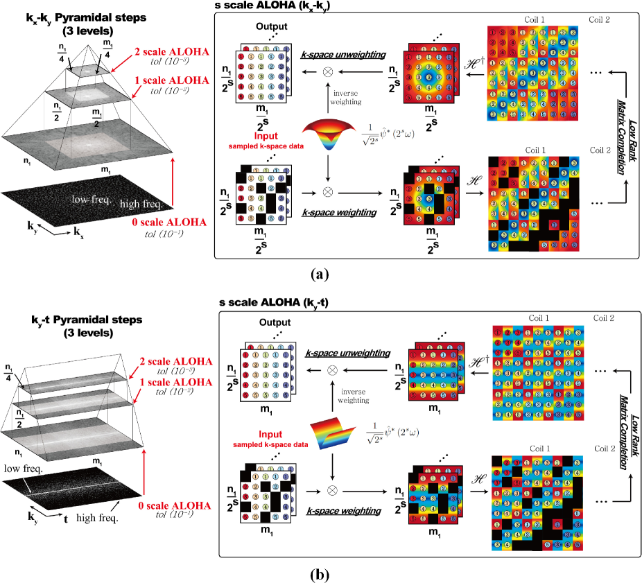
Figure 1: ALOHA implementation using pyramidal decomposition. Construction of Hankel matrices from (a) $k_{x}$-$k_{y}$ data by assuming that 2-D dydadic wavelet transform of images is sparse, and (b) $k-t$ subsampled data by assuming that dynamic images can be sparsified using spatial wavelet and temporal Fourier transform. In the box, each reconstruction unit at the $s$-scale (the $s$-scale ALOHA) is illustrated, which consists of five steps: (1) the k-space region extraction, (2) k-space element by element weighting using $s$-scale wavelet spectrum $\frac{1}{\sqrt{2^{s}}}\hat{\psi}(2^{s}\omega)$, (3) low-rank Hankel matrix completion, (4) k-space unweighting by dividing the interpolated k-space data using the $s$-scale wavelet spectrum, and (5) the k-space data replacement using the interpolated data. Note that for the case of dynamic MRI, one dimensional weigting is required along the phase encoding direction, whereas 2-D weighting is necessary for the case of static imaging. In the figure, $n_{1}$ denotes the ambient space dimension, and $\mathscr{H}^{\dagger}$ corresponds to the pseudo-inverse operation that takes the average value from the Hankel matrix and putting it back to the original k-space domain. The color coding in the Hankel structure matrix indicates the values of weighting.

Because the number of nonzero coefficient $f^{s}[l]$ is at most $k$, then the form of the righthand side equation (53) is similar to (10), so annihilating filters and the corresponding low-rank Hankel matrix can be found. However, one technical issue is that the righthand side of (54) has aliased copies of k-space data weighted by wavelet weighting. Therefore, the direct application of low rank matrix completion may not work. Accordingly, to deal with $2\pi/2^{s}$ repeating spectral structure, we propose a pyramidal decomposition of the Hankel structured matrix. More specifically, if the spectral component of $\hat{f}(\omega)$ is estimated for $|\omega|\geq\pi/2^{s}$, then we can constitute a residual signal recursively:

$$\hat{f}_{r}(\omega):=\left\{\begin{array}[]{ll}0,&|\omega|\geq\pi/2^{s}\\ \hat{f}(\omega),&\mbox{otherwise}\end{array}\right.$$ (57)

Then, for the corresponding discrete sample $f_{r}^{s}[l]:=\left.\langle f_{r},\psi_{s}(\cdot-x)\rangle\right|_{x=2^{s}l}$ with $f_{r}=\mathcal{F}^{-1}\{\hat{f}_{r}\}$, we have

$$\hat{f}_{r}^{s}(e^{i\omega}):=\sum_{l}f_{r}^{s}[l]e^{-i\omega 2^{s}l} = \frac{1}{\sqrt{2^{s}}}\hat{\psi}^{*}(2^{s}\omega)\hat{f}(\omega),$$ (58)

because its high frequency content will no more aliasing at a frequency inside $|\omega|\leq\pi/2^{s}$. Then, due to the sparsity of $f_{r}^{s}[l]$, there exists a filter that annihilates $\hat{\psi}^{*}(2^{s}\omega)\hat{f}(\omega)$. Consequently, the $s$-scale ALOHA problem can be formulated as

$$\min_{{\mathbf{m}}\in{\mathbb{C}}^{n_{1}/2^{s}}} \textsc{rank}\mathscr{H}({\mathbf{m}})$$

subject to $$P_{\Omega}({\mathbf{m}})=P_{\Omega}(\hat{\mathbf{l}}^{s}\odot\hat{\mathbf{f}}^{s})\ .$$

where

$$\hat{f}^{s}[n]=\left.\hat{f}(\omega)\right|_{\omega=n\pi/n_{1}},$$ (60)

and the weighting vector $\hat{\mathbf{l}}^{s}$ is composed of following spectral samples :

$$\hat{l}^{s}[n] = \left.\hat{l}^{s}(\omega)\right|_{\omega=n\pi/n_{1}}=\left.\frac{1}{\sqrt{2^{s}}}\hat{\psi}^{*}\left(2^{s}\omega\right)\right|_{\omega=n\pi/n_{1}},$$ (61)

where $n=-{n_{1}}/{2^{s+1}},\cdots,{n_{1}}/{2^{s+1}}-1$ and the superscript ^∗ denotes the complex conjugate. Note that sampling interval for $\hat{\psi}^{*}(\omega)$ widens by factor of 2 for each successive scale to construct the k-space weighting vector $\hat{\mathbf{l}}^{s}$. Consequently, we have a pyramidal decomposition as shown in Fig. 1, and the ALOHA (III-A) should be solved from the lowest scale, i.e. $s=0$, up to the highest scale (see caption of Fig. 1 for more discussion of the figures). Because sparsity can be imposed only on the wavelet coefficients, the low frequency k-space data that correspond to the scaling function coefficients should be acquired additionally during MR data acquisition. This information as well as the annihilating filter size then determines the the depth of the pyramidal decomposition as will be discussed in detail later.

There are several advantages of using wavelet approaches compared to the direct operator weighting in ALOHA framework. First, the pyramidal decomposition structure for low rank matrix completion can significantly reduce the overall computational complexity. Moreover, it has been observed in [36] that the wavelet approach is more robust for noise and the model mismatch, which is also consistently observed in ALOHA framework as will be discussed later.

Note that the proposed pyramidal scheme is an algorithm that is designed to approximately decouple the aliasing components in (54), and we do not claim the optimality of the proposed method. However, it is worth to mention that the optimality of a similar fine-to-coarse scale wavelet coefficients reconstruction was recently shown in Fourier compressed sensing problem [37].

III-B Generalization to Parallel MRI

Beside the annihilation property originating from sparsity in the transform domain, there exists an additional annihilation relationship that is unique in parallel MRI. The relationship we described here has similarity to SAKE and P-LORAKS when the image itself is sparse (even though these methods were inspired by the null space or GRAPPA type relationship), and our contribution is its generalization to transform domain sparse signals.

Specifically, in pMRI, the unknown image $g_{i}(x)$ from the $i$-th coil can be represented as

$$g_{i}(x)=s_{i}(x)f(x),\quad i=1,\cdots,r,$$

where $s_{i}(x)$ denotes the $i$-th coil sensitivity map, $f(x)$ is an unknown image, and $r$ denotes the number of coils. Then, for TV signals (i.e. $\mathrm{L}=\frac{d}{dx}$), we have

$$\mathrm{L}g_{i}(x) = s_{i}(x)\mathrm{L}f(x)+f(x)\mathrm{L}s_{i}(x)\ ,$$

whose Fourier transform is given by

$$\hat{l}(\omega)\hat{g}_{i}(\omega) = \hat{s}_{i}(\omega)\ast(\hat{l}(\omega)\hat{f}(\omega))+\hat{f}(\omega)\ast(\hat{l}(\omega)\hat{s}_{i}(\omega))\ .$$ (62)

Then, we can show the following inter-coil annihilating filter relationship:

Lemma 3.1.

Suppose that $\hat{h}(\omega)$ is the annihilating filter for $\hat{f}(\omega)$ such that $(\hat{h}\ast\hat{f})(\omega)=0$. Then, we have

$$\hat{h}(\omega)\ast\hat{s}_{j}(\omega)\ast\left(\hat{l}(\omega)\hat{g}_{i}(\omega)\right)-\hat{h}(\omega)\ast\hat{s}_{i}(\omega)\ast\left(\hat{l}(\omega)\hat{g}_{j}(\omega)\right)=0,\quad i\neq j.$$ (63)

Proof.

Using (62), we have

$$\hat{h}(\omega)\ast\hat{s}_{j}(\omega)\ast\left(\hat{l}(\omega)\hat{g}_{i}(\omega)\right) = \hat{h}(\omega)\ast\hat{s}_{j}(\omega)\ast\hat{s}_{i}(\omega)\ast(\hat{l}(\omega)\hat{f}(\omega))+\hat{h}(\omega)\ast\hat{s}_{j}(\omega)\ast\hat{f}(\omega)\ast(\hat{l}(\omega)\hat{s}_{i}(\omega))$$ (64)

$$= \hat{h}(\omega)\ast\hat{s}_{j}(\omega)\ast\hat{s}_{i}(\omega)\ast(\hat{l}(\omega)\hat{f}(\omega))$$

where the second term vanishes thanks to $(\hat{h}\ast\hat{f})(\omega)=0$. Similarly, we have

$$\hat{h}(\omega)\ast\hat{s}_{i}(\omega)\ast\left(\hat{l}(\omega)\hat{g}_{j}(\omega)\right) = \hat{h}(\omega)\ast\hat{s}_{i}(\omega)\ast\hat{s}_{j}(\omega)\ast(\hat{l}(\omega)\hat{f}(\omega))$$ (65)

Because Eqs. (64) and (65) are identical, Eq. (63) can be shown. Q.E.D. ∎

Therefore, to exploit the inter-coil annihilating property, Hankel matrix from each channel is stacked side by side to form a matrix $\mathcal{Y}$:

$$\mathcal{Y}=\begin{bmatrix}\mathscr{H}(\hat{\mathbf{l}}\odot\hat{\mathbf{g}}_{1})&\cdots&\mathscr{H}(\hat{\mathbf{l}}\odot\hat{\mathbf{g}}_{r})\end{bmatrix}\in{\mathbb{C}}^{(n_{1}-\kappa+1)\times\kappa r}\ ,$$ (66)

Here, the augmented matrix $\mathcal{Y}$ in (66) has the following rank condition:

Proposition 3.2.

For the concatenated Hankel matrix given in (66), we have

$$\mathrm{rank}~{}\mathcal{Y} \leq \frac{r(2k-r+1)}{2}\ .$$ (67)

where $k$ and $r$ denotes the sparsity and the number of coils, respectively.

Proof.

Since Eq. (63) holds for every pair among $r$-channels, it is easy to show that

$$\mathcal{Y}\mathcal{S}_{1}=\mathbf{0},$$

where $\mathcal{S}_{1}$ is defined recursively as follows:

$$\mathcal{S}_{r-1} \triangleq \left[\begin{array}[]{cc}\hat{\mathbf{v}}_{r}\\ -\hat{\mathbf{v}}_{r-1}\\ \end{array}\right]$$ (70)

$$\mathcal{S}_{t} \triangleq \left[\begin{array}[]{cccc|c}\hat{\mathbf{v}}_{t+1}&\hat{\mathbf{v}}_{t+2}&\cdots&\hat{\mathbf{v}}_{C}&\mathbf{0}\\ \hline\cr-\hat{\mathbf{v}}_{t}&&&&\\ &-\hat{\mathbf{v}}_{t}&&&\mathcal{S}_{t+1}\\ &&\ddots&\\ &&&-\hat{\mathbf{v}}_{t}&\end{array}\right]\ ,$$ (76)

wbere $\hat{\mathbf{v}}_{i}$ denotes the discrete samples of $\hat{h}(\omega)\ast\hat{s}_{i}(\omega)$. Accordingly,

$$\dim\textsc{Nul}(\mathcal{Y})\geq\mathrm{rank}(\mathcal{S}_{1})=\binom{r}{2}={r(r-1)}/{2}.$$

Furthermore, Proposition 2.1 informs us that $\mathscr{H}(\hat{\mathbf{l}}\odot\hat{\mathbf{g}}_{i})$ in $\mathcal{Y}$ has rank at most $k$. Therefore, we have

$$\mathrm{rank}~{}\mathcal{Y} \leq kr-\frac{r(r-1)}{2}=\frac{r(2k-r+1)}{2}\ .$$ (77)

∎

Due to the low-rankness of the concatenated matrix, the multichannel version of the ALOHA can be formulated as

$$\min_{\{{\mathbf{m}}_{i}\}_{i=1}^{r}} \textsc{rank}\begin{bmatrix}\mathscr{H}({\mathbf{m}}_{1})&\cdots&\mathscr{H}({\mathbf{m}}_{r})\end{bmatrix}$$

subject to $$P_{\Omega}({\mathbf{m}}_{i})=P_{\Omega}(\hat{\mathbf{l}}\odot\hat{\mathbf{g}}_{i}),\quad i=1,\cdots,r\ .$$

In addition, it is worth to emphasize the meaning of the rank condition of the concatenated matrix. Because the rank of $\mathcal{Y}$ is at most ${r(2k-r+1)}/{2}$ and there exist additional degrees of freedom that belong to the amplitudes of Diracs in the transform domain, the total degrees of the freedom for the FRI signal are at most $r(2k-r+1)$ [19, 20, 21]. In parallel MRI, if $m$ denotes the number of k-space sampling locations, then k-space data are sampled simultaneously from $r$-coils and the total number of k-space samples becomes $mr$. Since the number of the samples should be larger than the degree of the freedom, we have

$$mr\geq{r(2k-r+1)} \Longleftrightarrow k\leq\frac{m+r-1}{2}\ .$$ (79)

This result has very important geometric meaning. Suppose that we attempt to address parallel imaging by exploiting the joint sparsity. Using the notation in (1), this could be addressed by the following multiple measurement vector (MMV) problem

$$\min_{F} \|F\|_{0}$$

subject to $$G=AF$$ (80)

where $G=[{\mathbf{g}}_{1},\cdots,{\mathbf{g}}_{r}]$ and $F=[{\mathbf{f}}_{1},\cdots,{\mathbf{f}}_{r}]$ with ${\mathbf{f}}_{i}=[S_{i}]{\mathbf{f}}$ for a given sensitivity map $[S_{i}]$, and $\|\cdot\|_{0}$ denotes the number of non-zero rows. Then, it was shown in our previous work [22] and others [23, 24] that if $F_{*}$ satisfies $AF_{*}=G$ and

$$\|F_{*}\|_{0}<\frac{\mathrm{spark}(A)+\textsc{rank}(G)-1}{2}$$ (81)

then $F_{*}$ is the unique solution for $G=AF$, where $\mathrm{spark}(A)$ denote the smallest number of linearly dependent columns of $A$. For randomly chosen Fourier samples, we have $\mathrm{spark}(A)\geq m+1$. Moreover, $\textsc{rank}(G)=r$. Hence, (81) is equivalent to (79) if the unknown sparsity level is $k$, i.e. $\|F_{*}\|_{0}=k$.

Therefore, similar to the fact that single coil ALOHA does not lose any theoretical optimality compared to the single coil compressed sensing approaches, our ALOHA formulation for pMRI using (III-B) may fully exploit the multi-channel diversity from parallel acquisition. Moreover, because the k-space interpolation formulation of ALOHA is derived based on the information of the singularity of the signals, the resulting reconstruction results for both single and multi-channel formulation exhibit superior performance as will be discussed in experimental sections.

IV Implementation Details

IV-A 2D Hankel Structured Matrix Construction

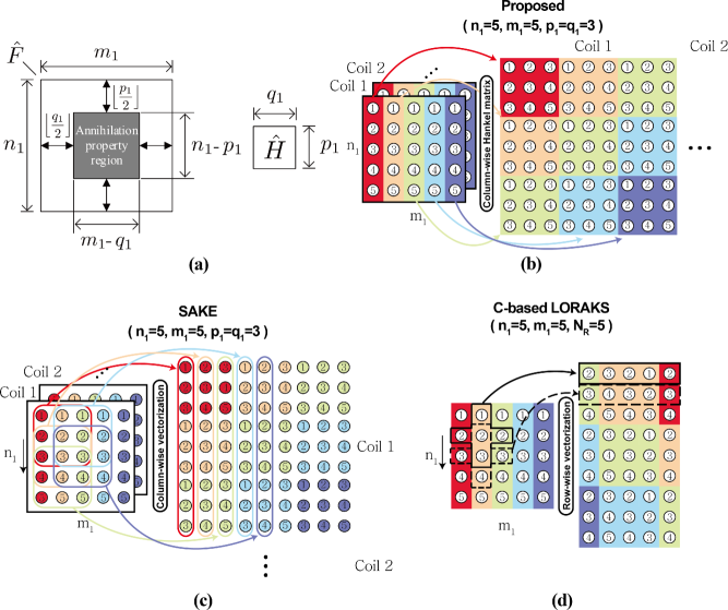
Figure 2: (a) Area where annihilation property holds. Various ways of constructing block Hankel matrices: (b) ALOHA, (c) SAKE, and (d) LORAKS. In (d), $N_{R}$ denotes the number of neighborhood pixels.

In 3D imaging or dynamic acquisition of MR data, the readout direction is usually fully sampled and the other two encoding directions are under sampled. Thus, this section presents an explicit way of constructing a 2D Hankel structured matrix. Specifically, if $\hat{h}[n,m]$ is a $p_{1}\times q_{1}$ size 2D annihilating filter, then the corresponding annihilating filter relation is given by

$$(\hat{h}\ast\hat{f})[n,m]=\sum_{i=0}^{p_{1}-1}\sum_{j=0}^{q_{1}-1}\hat{h}[i,j]\hat{f}[n-i,m-j]=0,$$ (82)

for all $n,m\in\Omega$. Let $n_{1}\times m_{1}$ k-space data matrix be defined by

$$\hat{F} := \begin{bmatrix}\hat{f}[0,0]&\cdots&\hat{f}[0,m_{1}-1]\\ \vdots&\ddots&\vdots\\ \hat{f}[n_{1}-1,0]&\cdots&\hat{f}[n_{1}-1,m_{1}-1]\end{bmatrix}$$

$$= \begin{bmatrix}\hat{\mathbf{f}}_{0}&\cdots&\hat{\mathbf{f}}_{m_{1}-1}\end{bmatrix}$$

Similarly, we define $p_{1}\times q_{1}$ annihilating filter matrix $\hat{H}$. Then, by removing the boundary effect from the 2D convolution as shown in Fig. 2(a), the 2D annihilation property should hold only inside of the domain and (82) can be equivalently represented as

$$\mathscr{H}(\hat{F})\hat{\bm{\mathfrak{h}}}=\mathbf{0},$$ (83)

where a 2-D Hankel structured matrix $\mathscr{H}(\hat{F})$ is constructed as

$$\!\left[\!\begin{array}[]{cccc}\!\mathscr{H}(\hat{\mathbf{f}}_{0})&\mathscr{H}(\hat{\mathbf{f}}_{1})&\cdots&\mathscr{H}(\hat{\mathbf{f}}_{q_{1}-1})\\ \mathscr{H}(\hat{\mathbf{f}}_{1})&\mathscr{H}(\hat{\mathbf{f}}_{2})&\cdots&\mathscr{H}(\hat{\mathbf{f}}_{q_{1}})\\ \vdots&\vdots&\ddots&\vdots\\ \mathscr{H}(\hat{\mathbf{f}}_{m_{1}-q_{1}})&\mathscr{H}(\hat{\mathbf{f}}_{m_{1}-q_{1}+1})&\cdots&\mathscr{H}(\hat{\mathbf{f}}_{m_{1}-1})\\ \end{array}\!\right]$$ (88)

with $\mathscr{H}(\hat{\mathbf{f}}_{j})\in{\mathbb{C}}^{(n_{1}-p_{1}+1)\times p_{1}}$ given by

$$\left[\begin{array}[]{cccc}\hat{f}[0,j]&\hat{f}[1,j]&\cdots&\hat{f}[p_{1}-1,j]\\ \hat{f}[1,j]&\hat{f}[2,j]&\cdots&\hat{f}[p_{1},j]\\ \vdots&\vdots&\ddots&\vdots\\ \hat{f}[n_{1}-p_{1},j]&\hat{f}[n_{1}-p_{1}+1,j]&\cdots&\hat{f}[n_{1}-1,j]\\ \end{array}\right]\ ,$$

and the annihilating filter vector is given by

$$\hat{\bm{\mathfrak{h}}}=\overline{\textsc{Vec}(\hat{H})}\ ,$$ (90)

where the overline denotes an operator that reserves the order of a vector. Using this, we can construct an augmented matrix $\mathcal{Y}$ in (66) from $r$-channels.

The augmented matrix structure $\mathscr{H}(\hat{F})$ illustrated in Fig. 2(b) is similar to those of SAKE and LORAKS/P-LORAKS in Fig. 2(c) and (d), respectively, with the following differences. Compared to SAKE, ALOHA stacks the multi-coil Hankel matrices side by side. Unlike the SAKE and ALOHA, LORAKS uses $R=4$ ($R$: neighborhood size) neighbors according to the software manual provided by the original authors. Moreover, the most important novelty of the proposed method is the k-space weighting to construct the Hankel structured matrix.

IV-B Hankel structured matrix completion algorithm

In order to solve Eqs. (II) and (III-B), we employ an SVD-free structured rank minimization algorithm [38] with an initialization using the low-rank factorization model (LMaFit) algorithm [39]. This algorithm does not use the singular value decomposition (SVD), so the computational complexity can be significantly reduced. Specifically, the algorithm is based on the following observation [40]:

$$\|A\|_{*}=\min\limits_{U,V:A=UV^{H}}\|U\|_{F}^{2}+\|V\|_{F}^{2}\quad\ .$$ (91)

Hence, (II) can be reformulated as the nuclear norm minimization problem under the matrix factorization constraint:

$$\min_{U,V:\mathscr{H}({\mathbf{m}})=UV^{H}} \|U\|_{F}^{2}+\|V\|_{F}^{2}$$

subject to $$P_{\Omega}({\mathbf{m}})=P_{\Omega}(\hat{\mathbf{f}}).$$ (92)

By combining the two constraints, we have the following cost function for an alternating direction method of multiplier (ADMM) step [41]:

$$L(U,V,{\mathbf{m}},\Lambda) := \iota({\mathbf{m}})+\frac{1}{2}\left(\|U\|_{F}^{2}+\|V\|_{F}^{2}\right)$$ (93)

$$+\frac{\mu}{2}\|\mathscr{H}({\mathbf{m}})-UV^{H}+\Lambda\|^{2}_{F}$$

where $\iota({\mathbf{m}})$ denotes an indicator function:

$$\iota({\mathbf{m}})=\left\{\begin{array}[]{ll}0,&\mbox{if $P_{\Omega}({\mathbf{m}})=P_{\Omega}(\hat{\mathbf{f}})$}\\ \infty,&\mbox{otherwise}\end{array}\right.\ .$$

One of the advantages of the ADMM formulation is that each subproblem is simply obtained from (93). More specifically, ${\mathbf{m}}^{(n+1)},U^{(n+1)}$ and $V^{(n+1)}$ can be obtained, respectively, by applying the following optimization problems sequentially:

$$\begin{array}[]{l}\min_{\mathbf{m}}\iota({\mathbf{m}})+\frac{\mu}{2}\|\mathscr{H}({\mathbf{m}})-U^{(n)}V^{(n)H}+\Lambda^{(n)}\|^{2}_{F}\\ \min_{U}\frac{1}{2}\|U\|_{F}^{2}+\frac{\mu}{2}\|\mathscr{H}({\mathbf{m}}^{(n+1)})-UV^{(n)H}+\Lambda^{(n)}\|^{2}_{F}\\ \min_{V}\frac{1}{2}\|V\|_{F}^{2}+\frac{\mu}{2}\|\mathscr{H}({\mathbf{m}}^{(n+1)})-U^{(n+1)}V^{H}+\Lambda^{(n)}\|^{2}_{F}\end{array}$$ (94)

and the Lagrangian update is given by

$$\Lambda^{(n+1)}= \mathcal{Y}^{(n+1)}-U^{(n+1)}V^{(n+1)H}+\Lambda^{(n)}\ .$$

It is easy to show that the first step in (94) can be reduced to

$${\mathbf{m}}^{(n+1)}=P_{\Omega^{c}}\mathscr{H}^{{\dagger}}\left\{U^{(n)}V^{(n)H}-\Lambda^{(n)}\right\}+P_{\Omega}(\hat{\mathbf{f}}),$$ (95)

where $P_{\Omega^{c}}$ is a projection mapping on the set $\Omega^{c}$ and $\mathscr{H}^{{\dagger}}$ corresponds to the Penrose-Moore pseudo-inverse mapping from our block Hankel structure to a vector. Hence, the role of the pseudo-inverse is taking the average value and putting it back to the original coordinate. Next, the subproblem for $U$ and $V$ can be easily calculated by taking the derivative with respect to each matrix, and we have

$$\begin{array}[]{l}U^{(n+1)}=\mu\left(\mathcal{Y}^{(n+1)}+\Lambda^{(n)}\right)V^{(n)}\left(I+\mu V^{(n)H}V^{(n)}\right)^{-1}\\ V^{(n+1)}=\mu\left(\mathcal{Y}^{(n+1)}+\Lambda^{(n)}\right)^{H}U^{(n+1)}\left(I+\mu U^{(n+1)H}U^{(n+1)}\right)^{-1}\end{array}$$ (96)

Note that the computational complexity of our ADMM algorithm is dependent on the matrix inversion in (96), whose complexity is determined by the estimated rank of the Hankel matrix. Therefore, even though the Hankel matrix has large size, the estimated rank is much smaller, which significantly reduces overall complexity.

Now, for faster convergence, the remaining issue is how to initialize $U$ and $V$. For this, we employ an algorithm called the low-rank factorization model (LMaFit) [39]. More specifically, for a low-rank matrix $Z$, LMaFit solves the following optimization problem:

$$\min_{U,V,Z}\frac{1}{2}\|UV^{H}-Z\|^{2}_{F}~{}\mbox{subject to }P_{I}(Z)=P_{I}(\mathscr{H}(\hat{\mathbf{f}}))$$ (97)

and $Z$ is initialized with $\mathscr{H}(\hat{\mathbf{f}})$ and the index set $I$ denotes the positions where the elements of $\mathscr{H}(\hat{\mathbf{f}})$ are known. LMaFit solves a linear equation with respect to $U$ and $V$ to find their updates and relaxes the updates by taking the average between the previous iteration and the current iteration. Moreover, the rank estimation can be done automatically. LMaFit uses QR factorization instead of SVD, so it is also computationally efficient. Even though the problem (97) is non-convex due to the multiplication of $U$ and $V$, the convergence of LMaFit to a stationary point was analyzed in detail [39]. However, the LMaFit alone cannot recover the block Hankel structure, which is the reason we use an ADMM step afterward to impose the structure.

IV-C Reconstruction Flow

As shown in Fig. 1, the ALOHA framework is comprised with several major steps: pyramidal decomposition, k-space weighting, Hankel matrix formation, rank estimation, SVD-free low rank matrix completion, and k-space unweighting. Here, we will explain these in more detail.

The pyramidal decomposition is performed as follows. First, in static MR data acquisition illustrated in Fig. 1(a), the $k_{x}-k_{y}$ corresponds to the two phase encoding directions that are downsampled. Thus, the Hankel matrix is constructed from $k_{x}-k_{y}$ data. After a k-space interpolation from a finer scale, the data at the current scale is defined to contain one-fourth of data around zero frequency from that of the previous scale. Second, in the case of dynamic MR imaging shown in Fig. 1(b), $k_{x}$ samples from the readout direction are fully acquired, whereas the $k_{y}$ directional phase encoding are downsampled along the temporal direction $t$. Therefore, the data in $k_{y}-t$ space (or simply, $k-t$ space) are downsampled, from which we construct a Hankel structure matrix. In pyramidal decomposition, after a k-space interpolation from a finer scale, the $k_{y}-t$ data in the current scale contains a half of the data from that of the previous scale. Note that the wavelet decomposition is performed only along the spatial domain, so the pyramidal decomposition is only performed along $k_{y}$ direction. This construction of Hankel matrix is due to the observation that the dynamic signal is sparse in spatial wavelet and temporal Fourier transform domain [42]. See more details in our recent work [42].

In both cases, the estimated k-space data at the lower scale are used to initialize the low rank matrix completion algorithm at the current scale. This accelerates the convergence speed. Moreover, due to the additional chance of refining the estimates, more important k-space samples at the low frequency regions are refined furthermore compared to the high frequency k-space samples. Consequently, the overall computational burden of the low rank matrix competition algorithm is significantly reduced while the overall quality is still maintained.

The k-space weighting is performed using wavelets. Specifically, based on our discussions on maximally localized smoothing function, we use a Haar wavelet expansion whose spectrum is given by

$$\hat{\psi}_{0}(\omega)=\frac{i\omega}{2}\left(\frac{\sin{\omega/4}}{\omega/4}\right)^{2}\exp\left(-i\frac{\omega}{2}\right) \ .$$ (98)

The corresponding k-space weighting at the $s$-scale is given by

$$\hat{l}_{s}(\omega)=\frac{1}{\sqrt{2^{s}}}\frac{i2^{s}\omega}{2}\left(\frac{\sin{2^{s}\omega/4}}{2^{s}\omega/4}\right)^{2}e^{-i\frac{2^{s}\omega}{2}}.$$

For the case of static MRI in Fig. 1(a), we use 2-D weighting by assuming that the image is sparse in 2-D dyadic wavelet transform domain. Care needs to be taken when applying the weighting to 2D Fourier domain because there are two frequency variables $(\omega_{x},\omega_{y})$. One could use a separable weighting $\hat{l}(\omega_{x},\omega_{y})=\hat{l}(\omega_{x})\hat{l}(\omega_{y})$; however, the resulting problem is that the missing k-space components along the frequency axis $\omega_{x}=0$ or $\omega_{y}=0$ cannot be recovered. Consequently, we applied the weighting sequentially along each axis, i.e. we solve (II) by applying $\hat{l}(\omega_{x})$ first, which is followed by solving (II) with $\hat{l}(\omega_{y})$. However, simultaneous weighting would be possible as demonstrated in a recent work for off-the-grid recovery of piecewise constant image [43]. For the case of dynamic imaging in Fig. 1(b), one dimensional weighting along the phase encoding direction was applied as explained in detail in [42]. Finally, after the k-space interpolation, the k-space unweighting is done in k-space pixel-by-pixel by dividing the reconstructed value with (98). Note that (98) has zero value at the DC frequency. However, because we acquire the DC value as well as some of the low frequency k-space data, the problem of dividing by zero never happened.

Because LORAKS is similar to the ALOHA without weighting, we use LORAKS as a reference to contrast why the proposed ALOHA framework has many advantages. The implementation of LORAKS was based on the source code available in the original author’s homepage, which requires manual setting of estimated ranks. We chose the rank for LORAKS that gave the best reconstruction quality. In Discussion, we also provided reconstruction results by ALOHA without weighting to control the confounds and confirm the importance of the k-space weighting in constructing Hankel matrix.

We used TITAN GTX graphic card for graphic processor unit (GPU) and i7-4770k CPU and the codes were written in MATLAB 2015a (Mathwork, Natick). To accelerate the algorithm, most part of the MATLAB codes were implemented using Compute Unified Device Architecture (CUDA) for GPU.

IV-D MR Acquisition and Reconstruction Parameters

To assess the performance of ALOHA for single coil compressed sensing imaging, k-space raw data from an MR headscan was obtained with Siemens Tim Trio 3T scanner using balanced steady-state free precession (bSSFP) sequence. The acquisition parameters were as follows: TR/TE $=10.68/5.34\mbox{ms}$, $208\times 256$ acquisition matrix (partial Fourier factor 7/8, oversampling factor $50\%$), and number of slices is 104 with $2\mbox{mm}$ slice thickness. The field-of-view (FOV) was $178\times 220\mbox{mm}^{2}$. We used the central coronal slice.

A retrospective down-sampling mask was generated according to a two dimensional Gaussian distribution and the data at the central $7\times 7$ region around zero frequency were obtained additionally. This is equivalent to assume a 3D imaging scenario where the readout direction is fully sampled and the downsampling is done in the remaining 2-D phase encoding direction. Downsampling factors of four was used to generate sampling masks. However, data was obtained as partial Fourier measurements, so effective downsampling ratio was 4.13. The 2-D k-space weighting using (98) was used. The ALOHA reconstruction was conducted using the following parameters: three levels of pyramidal decomposition, and decreasing LMaFit tolerance values ($5\times 10^{-2},5\times 10^{-3},5\times 10^{-4}$) at each level of the pyramid. In addition, an initial rank estimate for LMaFit started with one and was refined automatically in an increasing sequence, the annihilating filter size was 23$\times$23, and the ADMM parameter was $\mu=10^{3}$.

For the compressed sensing approach, we used two approaches with the same data and the same sampling masks: (1) the sparsity in wavelet domain (which we denote $l_{1}$-wavelet) [3], and (2) the split Bregman method for the total variation [44]. In case of $l_{1}$-wavelet approach, we implemented an ADMM algorithm using wavelet domain sparsity. In addition, for comparison with the existing state-of-the art approach using Hankel structured matrix completion algorithm, LORAKS was compared. In particular, C-based LORAKS was chosen because it exploits the image domain sparsity. The parameters for the $l_{1}$-wavelet and TV approaches were optimized to have the best performance in terms of the normalized mean square error (NMSE), which is defined by $\mbox{NMSE}({\mathbf{x}})={\|{\mathbf{x}}-{\mathbf{y}}\|_{2}^{2}}/{\|{\mathbf{y}}\|_{2}^{2}}$, where ${\mathbf{x}}$ and ${\mathbf{y}}$ denote the reconstructed and the ground-truth images, respectively. The LORAKS parameters were chosen manually to give the best reconstruction quality.

To evaluate the performance of ALOHA in static parallel imaging, k-space raw data from an MR headscan was obtained with Siemens Verio 3T scanner using 2D SE sequence. The acquisition parameters were as follows: TR/TE $=4000/100\mbox{ms}$, $256\times 256$ acquisition matrix, and six z-slices with $5\mbox{mm}$ slice thickness. The field-of-view (FOV) was $240\times 240\mbox{mm}^{2}$, and the number of coils was four. Retrospectively undersampled 2-D k-space data at the acceleration factor of eight were obtained according to a two dimensional Gaussian distribution in addition to the $7\times 7$ central region around zero frequency. The data from 4 receiver coils were used. For comparison, we used the identical data and sampling masks for SAKE [16], and SAKE with ESPIRiT [45]. Note that GRAPPA [13] requires ACS lines, so with the additional 50 samples along ACS, the effective downsampling ratio was 4.785, which is not good as the eight time acceleration in other algorithms. SAKE and SAKE with ESPIRiT are both low rank matrix completion algorithms for Hankel structured matrix collected from the whole k-space data. However, SAKE with ESPIRiT reduces the computational burden of the original SAKE by performing low rank matrix completion only for the $65\times 65$ central region with $7\times 7$ filter, after which coil sensitivities are estimated using the reconstruction data. The estimated coil sensitivities are used to estimate the remaining k-space missing data through ESPIRiT [45]. The parameters for SAKE and SAKE with ESPIRiT were chosen such that they provided the best reconstruction results. The parameters for the ALOHA are as follows: three levels of pyramidal decomposition with decreasing LMaFit tolerances ($10^{-1},10^{-2},10^{-3}$), and 7$\times$7 annihilating filter. The same LMaFit rank estimation strategy and ADMM parameter used for single coil experiments were employed. We generated the square root of sum of squares (SSoS) image from multi-coil reconstructions.

We also validated the performance of ALOHA for accelerated dynamic cardiac data in the $k-t$ domain. A cardiac cine data set was acquired using a 3T whole-body MRI scanner (Siemens; Tim Trio) equipped with a 32-element cardiac coil array. The acquisition sequence was bSSFP and prospective cardiac gating was used. The imaging parameters were as follows: FOV$=300\times 300\mbox{mm}^{2}$, acquisition matrix size$=128\times 128$, TE/TR $=1.37/2.7\mbox{ms}$, receiver bandwidth $=1184\mbox{Hz/pixel}$, and flip angle $=40^{\circ}$. The number of cardiac phases was 23 and the temporal resolution was 43.2ms. The k-t space samples including four lines around zero frequency were retrospectively obtained at the reduction factor of eight according to a Gaussian distribution. For comparison, k-t FOCUSS [7], LORAKS [17], and SAKE [16] was used. In case of LORAKS (single coil) and SAKE (multi coil), these algorithms were applied to k-t domain for dynamic reconstruction. The parameters in k-t FOCUSS, LORAKS, and SAKE, were selected to give the best NMSE values. For the ALOHA in single coil data, the following parameters were used: three level of pyramidal decomposition only along the phase encoding direction, decreasing LMaFit tolerances ($10^{-1},10^{-2},10^{-3}$) at each scale, and 17$\times$5 annihilating filter. The same LMaFit rank estimation strategy and ADMM parameter was $\mu=10$. The k-space weighting in Eq. (98) was applied only along the phase encoding direction.

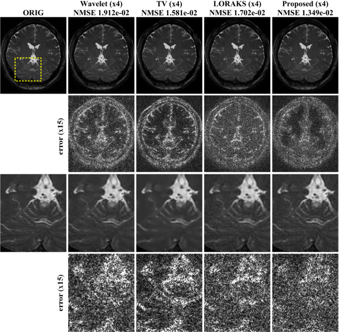
Figure 3: Comparison with $l_{1}$-wavelet compressed sensing, TV compressed sensing, LORAKS, and the proposed method at four fold acceleration factors. The data was acquired from a single channel coil. The first row shows reconstructed images, and the second row shows difference images between the ground-truth and the reconstructions, and the third row shows the magnified views of distorted regions in the reconstructed images. The last row shows the difference images in the magnified views.

Next, we investigated the synergetic improvement of dynamic imaging from multi-channel acquisition. Four representative coils out of 32 were used. The reason we chose only four coils was to verify that the generalised ALOHA can maximally exploit the multi-channel diversity even with the small number of coils. The four coils were chosen such that it covers every area of images. The same four coils were used for all algorithms for fair comparison. In the ALOHA, the annihilating filter size was $7\times 7$. The same LMaFit rank estimation strategy and ADMM parameter used before were employed. After the reconstructions of k-space samples, the inverse Fourier transform was applied, and the SSoS images were obtained by combining the reconstructed images.

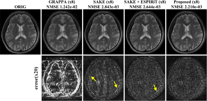
Figure 4: Parallel imaging results using GRAPPA, SAKE, SAKE with ESPIRiT and the proposed method at 8 fold acceleration. The second row shows the difference images. Areas with systematic artefacts are indicated by yellow arrows. Note that GRAPPA requires ACS lines, so with the additional 50 samples along ACS, the effective downsampling ratio was 4.785.

V Results

V-A Static MR experiments

Reconstructed results from a single coil brain data are shown in Fig. 3 with the NMSE values. From the NMSE values, we observed that the performance ALOHA was quantitatively superior to the performance of $l_{1}$-wavelet and TV based compressed sensing approach. The reconstruction results by ALOHA has less perceivable distortion compared to those of $l_{1}$-wavelet and TV approaches. This can be easily observed from the difference images in the second and the fourth rows of Fig. 3. In the case of $l_{1}$-wavelets and TV, structural distortion around the image edges was easily recognizable. In the last row of Fig. 3, the edges were reconstructed accurately by ALOHA. On the other hand, the contrast between grey matters and white matters in $l_{1}$-wavelets and TV reconstruction were significantly distorted compared with that of ALOHA. The LORAKS reconstruction appeared better than that of $l_{1}$-wavelets and TV reconstruction, but there were still remaining errors around the edges and the NMSE value was much higher than that of ALOHA.

Figure 5: Reconstruction results from 8 fold accelerated k-space data using (a) single coil and (b) four coils data set. Purple lines denote the regions corresponding to y-t cross sections that are magnified along temporal axis. The second rows in both (a) and (b) show the difference images between the ground-truth and the reconstructions.

Next we compared our parallel imaging results with those of the existing approaches for additional multichannel brain data set. The NMSE results in Fig. 4 showed that ALOHA was most accurate. From the difference images at the second row of Fig. 4, we observed that proposed method provided reconstruction results more accurately than other algorithms. In SAKE, the structures were distorted around the inner skull and the boundaries of tissues. In SAKE with ESPIRiT, overall reconstruction errors were higher than those from ALOHA and there were still remaining errors around the skull. The reconstruction time was 22.2sec with our preliminary GPU implementation of ALOHA, which attained a speed-up factor of 5 compared to CPU implementation. On the other hand, the computational time for MATLAB version of GRAPPA, SAKE, and SAKE+ESPIRiT were 9s, 320.4s, and 21.6s, respectively.

V-B Dynamic MR experiments

Using the sub-sampled k-space data at the acceleration factor of eight, the average NMSE values of k-t FOCUSS, LORAKS, and ALOHA, were $1.616\times 10^{-2}$, $1.363\times 10^{-2}$, and, $1.151\times 10^{-2}$, respectively. The sub-sampled data was collected according to a Gaussian distribution and included the four center lines around zero frequency. The average NMSE values were calculated using all temporal frames. These results confirmed that the proposed method outperformed k-t FOCUSS and LORAKS. As shown in Fig. 5(a), the temporal profile (indicated as a broken purple line) of the proposed reconstruction provided more accurate structures especially in the systole phase that were comparable to the true one, whereas the temporal variation in the k-t FOCUSS and LORAKS reconstruction became smoother and more blurry along the temporal dimension.

The NMSE values of the parallel dynamic imaging results from k-t FOCUSS, SAKE, and the proposed method using four coil k-space data were $8.75\times 10^{-3}$, $4.983\times 10^{-3}$ and $3.436\times 10^{-3}$, respectively, which quantitatively showed that the proposed method outperformed k-t FOCUSS and SAKE. Reduced residual artifacts were perceivable in the ALOHA difference images in Fig. 5(b). Moreover, the temporal profiles of the proposed reconstruction showed more accurate structures which were comparable to the true one, whereas the dynamic slice profile from k-t FOCUSS and SAKE showed smoother and more blurry transition. In particular, the proposed algorithm resulted in more accurate reconstructions of dynamic changes at the heart wall in the systole phase as shown in Fig. 5(b).

VI Discussion

VI-A Effects of k-space weighting

Figures 6(a)(b) illustrate the effects of wavelet weighting schemes. In order to also demonstrate the sensitivity with respect to annihilating filter size, we calculated the NMSE values by changing the filter size. Furthermore, to decouple the confounds originated from different implementation of C-based LORAKS and the ALOHA, the experimental results were generated using the same ALOHA framework with identical parameter setting, except for those related to the weighting. Figure 6(a) showed the single channel brain reconstruction results at the acceleration factor of 6. With weighting, the ALOHA reconstruction was conducted using the following parameters: three levels of pyramidal decomposition, and decreasing LMaFit tolerance values ($5\times 10^{-2},5\times 10^{-3},5\times 10^{-4}$) at each level of the pyramid. In addition, an initial rank estimate for LMaFit started with one and was refined automatically in an increasing sequence, and the ADMM parameter was $\mu=10^{3}$. Note that these parameters were same with those for (3). For the case of non-weighted implementation of ALOHA, the other parameters are exactly the same except the weighting. The results showed that the NMSE values of the weighted ALOHA are consistently better than those of unweighted ALOHA regardless of the annihilating filter size. Moreover, the NMSE values were not sensitive to the annihilating filter size for the cases of the proposed ALOHA, whose NMSE values converged. The reconstruction results from two implementation at the minimum NMSE values (marked as stars in Figures 6(a)(b) ) were illustrated, which again clearly showed that the residual errors of the weighted ALOHA is significantly smaller than the unweighted version of ALOHA.

Similar results were obtained from the dynamic cardiac imaging data in Figure 6(b). With weighting, the ALOHA reconstruction was conducted using the following parameters: three levels of pyramidal decomposition, and decreasing LMaFit tolerance values ($10^{-1},10^{-2},10^{-3}$) at each level of the pyramid. In addition, an initial rank estimate for LMaFit started with one and was refined automatically in an increasing sequence, and the ADMM parameter was $\mu=10$. The reconstruction parameters for the unweighted implementation of ALOHA were exactly the same except the weighting. The results showed that the unweighted ALOHA is very sensitive to the annihilating filter size, which showed the divergent behavior as the filter size increases. However, the proposed weighted ALOHA exhibited the convergent behaviors. This result clearly confirmed Proposition 2.1 saying that the low rank structure is invariant as long as the annihilating filter size is bigger than the transform domain sparsity level. The reconstruction results at the minimum NMSE values clearly showed that the proposed approach provided more clearly transition between diastole and systole phases.

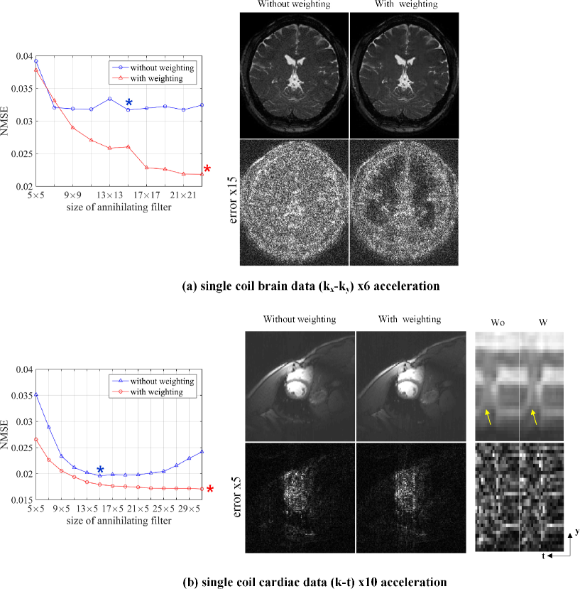
Figure 6: The effect of weighting and annihilating filter size in ALOHA implementation. (a) Single coil brain data results, and (b) single coil dynamic cardiac imaging results. The results clearly showed that the weighting is necessary for ALOHA to exploit the transform domain sparsity. On the other hand, the unweighted implementation exhibited divergent behavior with increasing filter size.

VI-B Hyper-Parameter Estimation

Figure 7: Reconstruction NMSE values with respect to different decomposition levels. The data is from single channel static MR reconstruction results in Fig. 3.

In order to show the importance of the pyramidal decomposition, Fig. 7 plots the computational time versus NMSE values of single coil brain data by changing the number of decomposition levels. As discussed before, the maximum decomposition level is determined by the acquired low frequency components and the annihilating filter size. In this data set, k-space dimension was $208\times 512$ and the annihilating filter size was $23\times 23$, and $7\times 7$ k-space data around zero frequency were acquired. By converting the Hankel matrix dimension in (88) for the $s$-scale, the number of rows should not be smaller than the number of columns; so we should impose constraint

$$n_{1}/2^{s}-p_{1}+1=208/2^{s}-23+1\geq 23,$$

where $s$ is the scale. This provides $s\leq 2$, and the maximum scale becomes 2. Fig. 7 showed that the performance gain increases as a scale increases; as expected, for $s\geq 3$, the performance improvement was negligible. Therefore, the maximum scale was determined as $s=2$.

The other important reconstruction parameters include the size of the annihilating filter, the number of iterations, and tolerances used in LMaFit algorithm. Recall that the annihilating filter size corresponds to the matrix pencil size in sensor array signal processing [34], and it should be set larger than the sparsity level of the transform coefficients. In fact, by considering the expression of $c_{s}$ in (41), the optimal annihilating filter size for 2D data is $n_{1}/2\times m_{1}/2$, where $n_{1}\times m_{1}$ denotes the full k-space data size. However, such large annihilating filter size introduces significant computational burden, so we tried to reduce the filter size as long as the image quality is not degraded. Based on extensive experiments, we found that in single coil image, the filter size should be set larger than that of parallel imaging, because the annihilating filter size is solely determined by the sparsity level. In parallel imaging, there exist additional annihilating filters from the intercoil relationship, so the annihilating filter size for each Hankel matrix construction can be set smaller than that of a single coil imaging.

Finally, the tolerance level for LMaFit, which corresponds to the fitting accuracy, plays key role in determining the initial rank estimate. The initial rank estimate need not be close to the exact rank, but it was used to define the dimension of $U$ and $V$ in ADMM. We found that the tolerance level could be determined by considering different noise contributions in k-space data. Specifically, higher frequency components are usually contaminated by higher level of noises compared to the low frequency k-space data, so the LMaFit fitting accuracy need not be enforced strictly. This was the case when LMaFit was applied at a lower scale, since high frequency k-space data are more weighted and noises were boosted. On the other hand, more accurate fitting is required for higher scale data where the lower frequency k-space data are more weighted. Consequently, we chose decreasing values of tolerances per scale for in-vivo experiments.

VI-C Concatenation Direction of Hankel Matrices for Parallel MRI

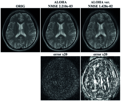
Figure 8: Dependency of concatenation direction of Hankel matrix for parallel MRI: (middle) side by side augmentation of Hankel matrices, and (right) vertical augmentation of Hankel matrices. Side-by-side augumentation provided the superior reconstruction results.

When generalizing the Hankel matrix model from single to multiple channels, we chose to stack the Hankel matrices corresponding to individual channels side by side. One could suggest stacking them one on top of another, which would represent a different matricization. Based on our discussion in Section II, in order to stack the Hankel matrix on top of another, the Hankel matrices should share the same annihilating filter. However, for the TV signal, the structure in (62) showed that it is not possible to find a common annihilating filter $\hat{h}_{c}(\omega)$ such that $\hat{h}_{c}(\omega)\ast\left(\hat{l}(\omega)\hat{g}_{i}(\omega)\right)=0,\forall i.$ On the other hand, the relationship in Eq. (63) clearly showed that there are inter-coil annihilating filters that can cancel out each combinations of the k-space signals. Therefore, to utilize (63), we should stack the Hankel matrix size by side.

To confirm the theoretical findings, we compared the reconstruction results from the two different stacking of Hankel matrices. As shown in Fig. 8, the vertical augmentation of Hankel matrices provided inferior reconstruction results compred to the side by side augmentation of Hankel matrices. This again confirmed the importance of the concatenation direction and the analysis by Proposition 3.2.

VI-D Further Extensions

Note that this work is a first step towards unifying sparse and low rank models, so there are many rooms for improvement. In particular, it could be extended for other measurement and sparsity models. For example, while Eq. (II) is based on a data equality constraint that focuses on standard Cartesian image reconstruction, we could convert $(P)$ in (II) to deal with the cases of general non-Cartesian imaging and/or noisy measurements:

$$(P^{\prime}) \min_{{\mathbf{m}}\in{\mathbb{C}}^{n}} \textsc{rank}\mathscr{H}({\mathbf{m}})$$

subject to $$\|P_{\Omega}({\mathbf{m}})-A_{\Omega}(\hat{\mathbf{l}}\odot\hat{\mathbf{f}})\|\leq\delta\ ,$$

where ${\mathbf{m}}$ denotes the spectrum data on cartesian grid, $A_{\Omega}$ denotes a linear mapping that interpolates non-cartesian data $\hat{\mathbf{l}}\odot\hat{\mathbf{f}}$ to the nearest cartesian grid index $\Omega$, and the noisy level $\delta$ is determined by the gridding or measurement noises. The minimization problem $(P^{\prime})$ can be also addressed using an SVD-free ADMM approach similar to (93), except that the indicator function-based data fidelity term is changed to $l_{2}$ data fidelity term. The detailed algorithm is described in [28].

In addition, ALOHA could be extended for reconstruction models that incorporate various system non-idealities. For example, in our recent work [46], we showed that EPI ghost artifacts that originate from off-resonance related inconsistencies between odd and even echoes can be removed by exploiting that the differential k-space data between the even and odd echoes is a Fourier transform of an underlying sparse image. Specifically, we can construct a rank-deficient concatenated Hankel structured matrix from even and odd k-space data, whose missing data can be interpolated using ALOHA. However, the extension of ALOHA for general off-resonance corrected MR reconstruction is still an open problem, which needs a further investigation in the future.

While this paper assumes that signals can be sparsified using dyadic wavelet ransforms, in general, signals can be more easily sparsified using non-decimated redundant wavelets. In this case, the corresponding non-decimated discrete sample at the $s$-scale is given by $f^{s}[l]:=\left.\langle f,\psi_{s}(\cdot-x)\rangle\right|_{x=l}$ whose spectrum can be represented by

$$\hat{f}^{s}(e^{i\omega}):=\sum_{l}f^{s}[l]e^{-i\omega l} = \frac{1}{\sqrt{2^{s}}}\hat{\psi}^{*}(2^{s}\omega)\hat{f}(\omega).$$ (100)

Because there exists no aliasing components due to the lack of downsampling, the construction of weighted Hankel matrix is much simpler than the dyadic wavelet transform. However, one of the potential downsides is that the number of non-zero wavelet transform coefficients $f^{s}[l]$ increases up to $2^{s}k$. Therefore, more k-space measurements are required to recover k-space data corresponding to the coarse scale wavelet coefficients. One potential solution would be to utilize the recovered high frequency k-space samples as additional measurements for interpolating the coarser level k-space samples. Note that this is different from dyadic wavelet case which discards higher frequency k-space samples in recovering low frequency k-space samples. However, the efficacy of this proposal needs to be evaluated systematically, which is beyond the scope of this paper.

Other than wavelet or TV representation, modern compressed sensing approach deals with advanced sparsifying transforms such as patch-based methods, dictionary learning, Markov penalties, and so on. The extension of ALOHA for such model would be important and rewarding, which requires more extensive investigation in subsequent research. Recently, ALOHA was successfully used for MR parameter mapping [42]. Considering recent success of direct parameter mappings [47, 48], the extension of ALOHA for direct parameter mapping would be very interesting, which deservers further investigations in the future.

VII Conclusion

In this paper, we proposed a general framework for annihilating filter based low-rank Hankel matrix approach (ALOHA) for static and dynamic MRI inspired by recent calibration-free k-space methods such as SAKE and LORAKS/P-LORAKS. Because natural images can be much more effectively sparsified in the transform domains, we generalized the idea to include signals that can be sparsfied in the transform domains. Our analysis showed that the transform domain sparsity can be equivalently represented as low-rank Hankel structured matrix in the weighted k-space domain, whose weighting function is determined solely by the transform, not by the data. In particular, when signals are effectively sparsified in dyadic wavelet transform, the corresponding low rank Hankel matrix completion problem can be implemented using a pyramidal decomposition, which significantly reduces the overall computational complexity and improves the noise robustness. For parallel imaging data, we verified that by stacking Hankel matrix from each coil side by side, we may fully exploit the coil sensitivity diversity thanks to existence of inter-coil annihilating filters.

Reconstruction results from single coil static MR imaging confirmed that the proposed method outperformed the existing compressed sensing framework with TV regularization. We further demonstrated superior performance of the proposed method in static parallel MR imaging even without calibration data. Furthermore, the algorithm was successfully extended to dynamic accelerated MRI along k-t domain with both single coil and multi coil dynamic MR data. Therefore, we concluded that the proposed algorithm was very effective in unifying the compressed sensing and parallel MRI.

References

- [1] D. L. Donoho, “Compressed sensing,” IEEE Trans. Inf. Theory, vol. 52, no. 4, pp. 1289–1306, 2006.
- [2] E. J. Candès, J. Romberg, and T. Tao, “Robust uncertainty principles: Exact signal reconstruction from highly incomplete frequency information,” IEEE Trans. Inf. Theory, vol. 52, no. 2, pp. 489–509, 2006.
- [3] M. Lustig, D. Donoho, and J. M. Pauly, “Sparse MRI: The application of compressed sensing for rapid MR imaging,” Magn. Reson. Med., vol. 58, no. 6, pp. 1182–1195, 2007.
- [4] D. Liang, B. Liu, J. Wang, and L. Ying, “Accelerating SENSE using compressed sensing,” Magn. Reson. Med., vol. 62, no. 6, pp. 1574–1584, 2009.
- [5] J. P. Haldar, D. Hernando, and Z.-P. Liang, “Compressed-sensing MRI with random encoding,” IEEE Trans. Med. Imag., vol. 30, no. 4, pp. 893–903, 2011.
- [6] S. S. Vasanawala, M. T. Alley, B. A. Hargreaves, R. A. Barth, J. M. Pauly, and M. Lustig, “Improved pediatric MR imaging with compressed sensing 1,” Radiology, vol. 256, no. 2, pp. 607–616, 2010.
- [7] H. Jung, K. Sung, K. S. Nayak, E. Y. Kim, and J. C. Ye, “k-t FOCUSS: A general compressed sensing framework for high resolution dynamic MRI,” Magn. Reson. Med., vol. 61, no. 1, pp. 103–116, 2009.
- [8] H. Jung, J. Park, J. Yoo, and J. C. Ye, “Radial k-t FOCUSS for high-resolution cardiac cine MRI,” Magn. Reson. Med., vol. 63, no. 1, pp. 68–78, 2010.
- [9] H. Yoon, K. Kim, D. Kim, Y. Bresler, and J. Ye, “Motion adaptive patch-based low-rank approach for compressed sensing cardiac cine MRI,” IEEE Trans. Med. Imag., vol. 33, no. 11, pp. 2069–2085, Nov 2014.
- [10] S. G. Lingala, Y. Hu, E. DiBella, and M. Jacob, “Accelerated dynamic MRI exploiting sparsity and low-rank structure: kt SLR,” IEEE Trans. Med. Imag., vol. 30, no. 5, pp. 1042–1054, 2011.
- [11] T. Çukur, M. Lustig, and D. G. Nishimura, “Improving non-contrast-enhanced steady-state free precession angiography with compressed sensing,” Magn. Reson. Med., vol. 61, no. 5, pp. 1122–1131, 2009.
- [12] K. P. Pruessmann, M. Weiger, M. B. Scheidegger, P. Boesiger et al., “SENSE: sensitivity encoding for fast MRI,” Magn. Reson. Med., vol. 42, no. 5, pp. 952–962, 1999.
- [13] M. A. Griswold, P. M. Jakob, R. M. Heidemann, M. Nittka, V. Jellus, J. Wang, B. Kiefer, and A. Haase, “Generalized autocalibrating partially parallel acquisitions (GRAPPA),” Magn. Reson. Med., vol. 47, no. 6, pp. 1202–1210, 2002.
- [14] K. P. Pruessmann, “Encoding and reconstruction in parallel MRI,” NMR in Biomedicine, vol. 19, no. 3, pp. 288–299, 2006.
- [15] M. Lustig and J. M. Pauly, “SPIRiT: Iterative self-consistent parallel imaging reconstruction from arbitrary k-space,” Magn. Reson. Med., vol. 64, no. 2, pp. 457–471, 2010.
- [16] P. J. Shin, P. E. Larson, M. A. Ohliger, M. Elad, J. M. Pauly, D. B. Vigneron, and M. Lustig, “Calibrationless parallel imaging reconstruction based on structured low-rank matrix completion,” Magn. Reson. Med., vol. 72, no. 4, pp. 959–970, 2014.
- [17] J. Haldar, “Low-rank modeling of local k-space neighborhoods (LORAKS) for constrained MRI,” IEEE Trans. Med. Imag., vol. 33, no. 3, pp. 668–681, March 2014.
- [18] J. P. Haldar and J. Zhuo, “P-LORAKS: Low-rank modeling of local k-space neighborhoods with parallel imaging data,” Magn. Reson. Med., 2015.
- [19] M. Vetterli, P. Marziliano, and T. Blu, “Sampling signals with finite rate of innovation,” IEEE Trans. Signal Process., vol. 50, no. 6, pp. 1417–1428, 2002.
- [20] P. L. Dragotti, M. Vetterli, and T. Blu, “Sampling moments and reconstructing signals of finite rate of innovation: Shannon meets Strang–Fix,” IEEE Trans. Signal Process., vol. 55, no. 5, pp. 1741–1757, 2007.
- [21] I. Maravic and M. Vetterli, “Sampling and reconstruction of signals with finite rate of innovation in the presence of noise,” IEEE Trans. Signal Process., vol. 53, no. 8, pp. 2788–2805, 2005.
- [22] J. M. Kim, O. K. Lee, and J. C. Ye, “Compressive MUSIC: revisiting the link between compressive sensing and array signal processing,” IEEE Trans. Inf. Theory, vol. 58, no. 1, pp. 278–301, 2012.
- [23] K. Lee, Y. Bresler, and M. Junge, “Subspace methods for joint sparse recovery,” IEEE Trans. Inf. Theory, vol. 58, no. 6, pp. 3613–3641, 2012.
- [24] M. E. Davies and Y. C. Eldar, “Rank awareness in joint sparse recovery,” IEEE Trans. Inf. Theory, vol. 58, no. 2, pp. 1135–1146, 2012.
- [25] M. Unser, P. D. Tafti, and Q. Sun, “A unified formulation of Gaussian versus sparse stochastic processes–Part I: Continuous-domain theory,” IEEE Trans. Inf. Theory, vol. 60, no. 3, pp. 1945–1962, 2014.
- [26] M. Unser, P. Tafti, A. Amini, and H. Kirshner, “A unified formulation of Gaussian versus sparse stochastic processes–Part II: Discrete-domain theory,” IEEE Trans. Inf. Theory, vol. 60, no. 5, pp. 3036–3051, 2014.
- [27] Y. Chen and Y. Chi, “Robust spectral compressed sensing via structured matrix completion,” IEEE Trans. Inf. Theory, vol. 60, no. 10, pp. 6576 – 6601, 2014.
- [28] J. C. Ye, J. M. Kim, and K. H. Jin, “Compressive sampling using annihilating filter-based low-rank interpolation,” arXiv preprint arXiv:1511.08975, 2015.
- [29] E. J. Candès and B. Recht, “Exact matrix completion via convex optimization,” Found. Comput. Math., vol. 9, no. 6, pp. 717–772, 2009.
- [30] J.-F. Cai, E. J. Candès, and Z. Shen, “A singular value thresholding algorithm for matrix completion,” SIAM Journal on Optimization, vol. 20, no. 4, pp. 1956–1982, 2010.
- [31] E. J. Candès and T. Tao, “The power of convex relaxation: Near-optimal matrix completion,” IEEE Trans. Inf. Theory, vol. 56, no. 5, pp. 2053–2080, 2010.
- [32] D. Gross, “Recovering low-rank matrices from few coefficients in any basis,” IEEE Trans. Inf. Theory, vol. 57, no. 3, pp. 1548–1566, 2011.
- [33] R. H. Keshavan, A. Montanari, and S. Oh, “Matrix completion from a few entries,” IEEE Trans. Inf. Theory, vol. 56, no. 6, pp. 2980–2998, 2010.
- [34] Y. Hua and T. K. Sarkar, “Matrix pencil method for estimating parameters of exponentially damped/undamped sinusoids in noise,” IEEE Trans. Acoust., Speech, Signal Process., vol. 38, no. 5, pp. 814–824, 1990.
- [35] S. Mallat, A wavelet tour of signal processing. Academic press, 1999.
- [36] M. Unser and P. D. Tafti, An introduction to sparse stochastic processes. Cambridge University Press, 2010.
- [37] Y. Zhang and P. L. Dragotti, “On the reconstruction of wavelet-sparse signals from partial Fourier information,” IEEE Signal Processing Letters, vol. 22, no. 9, pp. 1234–1238, 2015.
- [38] M. Signoretto, V. Cevher, and J. A. Suykens, “An SVD-free approach to a class of structured low rank matrix optimization problems with application to system identification,” in IEEE Conf. on Decision and Control, 2013.
- [39] Z. Wen, W. Yin, and Y. Zhang, “Solving a low-rank factorization model for matrix completion by a nonlinear successive over-relaxation algorithm,” Math. Prog. Comp., vol. 4, no. 4, pp. 333–361, 2012.
- [40] N. Srebro, “Learning with matrix factorizations,” Ph.D. dissertation, Dept, of Elect. Eng. and Comput. Sci., MIT, MA, 2004.
- [41] S. Boyd, N. Parikh, E. Chu, B. Peleato, and J. Eckstein, “Distributed optimization and statistical learning via the alternating direction method of multipliers,” Found. Trends in Mach. Learn., vol. 3, no. 1, pp. 1–122, 2011.
- [42] D. Lee, K. H. Jin, E. Y. Kim, S.-H. Park, and J. C. Ye, “Acceleration of MR parameter mapping using annihilating filter-based low rank Hankel matrix (ALOHA),” Magn. Reson. Med (in press), 2015.
- [43] G. Ongie and M. Jacob, “Off-the-grid recovery of piecewise constant images from few Fourier samples,” arXiv preprint arXiv:1510.00384, 2015.
- [44] T. Goldstein and S. Osher, “The split Bregman method for L1-regularized problems,” SIAM J. Imaging Sci., vol. 2, no. 2, pp. 323–343, 2009.
- [45] M. Uecker, P. Lai, M. J. Murphy, P. Virtue, M. Elad, J. M. Pauly, S. S. Vasanawala, and M. Lustig, “ESPIRiT-an eigenvalue approach to autocalibrating parallel MRI: Where SENSE meets GRAPPA,” Magn. Reson. Med., vol. 71, no. 3, pp. 990–1001, 2014.
- [46] J. Lee, K. H. Jin, and J. C. Ye, “Reference-free single-pass EPI Nyquist ghost correction using annihilating filter-based low rank Hankel matrix (ALOHA),” Magn. Reson. Med (in press), 2015.
- [47] J. V. Velikina, A. L. Alexander, and A. Samsonov, “Accelerating MR parameter mapping using sparsity-promoting regularization in parametric dimension,” Magnetic Resonance in Medicine, vol. 70, no. 5, pp. 1263–1273, 2013.
- [48] D. Ma, V. Gulani, N. Seiberlich, K. Liu, J. L. Sunshine, J. L. Duerk, and M. A. Griswold, “Magnetic resonance fingerprinting,” Nature, vol. 495, no. 7440, pp. 187–192, 2013.