Entanglement entropy of composite fermions realized by (deformed) fermions vs. that of composite bosons

In our two preceding papers we studied bipartite composite boson (or quasiboson) systems through their realization in terms of deformed oscillators. Therein, the entanglement characteristics such as the entanglement entropy and purity were found and expressed, for both one-quasiboson and more complex states, through the parameter of deformation. In this work we initiate an analogous study of composite fermions for two major cases: (i) “boson + fermion” composites; (ii) “deformed-boson + fermion” composites. Both the entanglement entropy and purity of composite fermions are dealt with, their dependence on the relevant parameters established, and for some particular two- or three-mode cases depicted graphically. In a few special cases the entanglement entropy turns out to be constant $S_{0}=\ln 2$ (or $\ln 3$) or $S_{0}=0$, while in the rest of the cases which we considered it varies between zero and $\ln 2$ (or $\ln 3$).

Keywords: composite fermions; composite bosons (quasi-bosons); realization by deformed oscillators; bipartite entanglement; entanglement entropy; purity

PACS: 05.30.Fk, 71.10.Pm, 02.20.Uw, 03.67.Mn, 03.65.Ud, 05.30.Jp, 11.10.Lm

1 Introduction

Composite fermions (CFs) play significant role in modern quantum physics. Suffice it to mention few distinct instances of CFs: one taken from the domain of condensed matter physics, namely quasiparticles involved in the theory of fractional quantum Hall effect [1], the other two – baryons and pentaquarks – belong to the realm of high energy physics [2, 3, 4]. In this paper we focus on the composite fermions with algebraic realization in two relatively simple cases: the first one involves, as the constituents, pure fermion and pure boson, while the second one concerns composites of pure fermion and a deformed boson, the description of the latter being taken in rather general form.

Not less important are the composite bosons (quasi-bosons, cobosons) i.e. non-elementary Bose-like systems or (quasi-)particles built from two or more constituent particles. These are as well widely encountered [5, 6, 2, 7, 8, 9, 10] in modern quantum physics, both theoretical and experimental. Among quasibosons there are excitons, cooperons, positronium, mesons, diquarks or tetraquarks, odd-odd or even-even nuclei, atoms, etc. In our preceding works [11, 12] we focused on the case of bipartite (two-component) composite bosons of two types: “fermion + fermion” and “boson + boson” ones such that their creation and annihilation operators are given through the typical ansatz,

$$A^{{\dagger}}_{\alpha}=\sum_{\mu\nu}\Phi_{\alpha}^{\mu\nu}a^{{\dagger}}_{\mu}b^{{\dagger}}_{\nu},\ \quad A_{\alpha}=\sum_{\mu\nu}\overline{\Phi_{\alpha}^{\mu\nu}}b_{\nu}a_{\mu},$$ (1)

with $a^{{\dagger}}_{\mu}$ and $b^{{\dagger}}_{\nu}$ the creation operators for the (distinguishable) constituents which can be taken as either both fermionic or both bosonic. In [13, 14] it was shown that the composite bosons of particular form (corresponding to an appropriate matrices $\Phi_{\alpha}^{\mu\nu}$) can be realized, in algebraic sense, by suitable deformed bosons (deformed oscillators). Note that, with such realization in mind, one can then construct certain deformed Bose gas model which serves for an effective description [15] of the non-Bose like behavior of two-particle correlation function intercepts of the pions $\pi^{+}$ and $\pi^{-}$ (also known as quark-antiquark composites) produced in the experiments on Heavy ion collisions at RHIC.

An important concept used in quantum information theory, quantum communication and teleportation [16, 5], is the notion of entanglement or quantum correlatedness between the constituents of composite particle or another composite system. This concept was recently actively studied just in the context of quasi-bosons [17, 18, 11]. Among the measures or witnesses characterizing the degree of entanglement, most widely used are the entanglement entropy and purity (= inverse of the Schmidt number) [16, 5]. The measures of entanglement between components of quasi-boson quantify to what extent or accuracy the quasiboson approaches the properties of true boson [17, 18, 19, 20].

For the composite bosons realizable by deformed oscillators it is possible to directly link [11] the relevant parameter of deformation with the entanglement characteristics of the composite boson. Then, the characteristics (or measures) of bipartite entanglement with respect to $a$- and $b$-subsystems, see the ansatz (1), can be found explicitly [11], and given through the deformation parameter: for single composite boson, for multi-quasiboson states, and for a coherent state corresponding to such quasi-bosons.

It is of importance to know what is the influence of system’s energy on the (variation of) quantum correlation and/or quantum statistics properties of the system under study. The energy of a quasi-boson differs from the energy of the respective ideal boson, and the difference (including quasiboson bound states energy) essentially depends on the quasi-boson’s entanglement, and thus the latter clearly shows the deviation from bosonic behavior. Let us note in this context that the entanglement-energy relation is relevant to quantum information research, quantum communication, entanglement production [21], quantum dissociation processes [10], particle addition or subtraction [22, 23]. In the case of composite bosons (quasi-bosons) it was explored in [12], and a number of interesting observations was obtained.

In this work we explore an alternative type of composites – the composite fermions. Since the entanglement entropy $S_{ent}$ is of primary interest, we below, after appropriate analysis of the realization issue, pay our main attention to finding the entanglement entropy $S_{ent}$ characterizing the composite fermion systems. Our treatment is performed for the one composite fermion states (for comparison, the respective results for one quasi-boson states are also briefly sketched). In some analogy with the case of quasi-bosons, we take the composite fermions as bipartite systems realized in terms of mode-independent fermionic oscillators (such independence is understood in fermionic sense). Let us also note that the other entanglement measure – purity – will be considered, where appropriate, as well.

Let us emphasize that the investigation in this paper concern a single (or isolated) composite fermion states, not many-fermion system in some region of space. Accordingly, the considered entanglement and its entropy incorporate the two parties (two constituents) of the bipartite composite fermion. Just these features make our approach and analysis basically different from some recent works on the entanglement entropy of a system of free or composite fermions, see e.g. [24, 25], where the size of subsystem played basic role, and the very entanglement was viewed in a way fully different from ours.

The paper is organized as follows. A sketch of main aspects on quasi-bosons is given in Sec. 2. Major part contained in Sections 3-6 deals with composite fermions. First of all, we perform the analysis of algebraic realization of composite fermions by means of (deformed) fermionic oscillators. Then, the entanglement entropy of such (one-particle) CF states is explored in Sec. 4-6. Modified CFs – those composed of fermion and deformed boson are analyzed in Sec. 5. The purity witness of bipartite entanglement of CF state is considered as well, see Section 4. The paper is concluded with short discussion of the essence of the obtained results, of some implications and possible developments.

2 Quasi-bosons formed as two-fermion (two-boson) composites

Let us recall main facts on the composite bosons realized by the set of independent modes of deformed bosons (deformed oscillators), given by the defining deformation structure function $\varphi(n)$. At the algebraic level the quasiboson operators $A_{\alpha}$, $A^{\dagger}_{\alpha}$ and the number operator $N_{\alpha}$ satisfy on the states the same relations as the corresponding deformed oscillator creation/annihilation and occupation number operators:

$$A^{\dagger}_{\alpha}A_{\alpha}=\varphi(N_{\alpha}),$$ (2)

$$[A_{\alpha},A^{\dagger}_{\beta}]=\delta_{\alpha\beta}\bigl{(}\varphi(N_{\alpha}+1)-\varphi(N_{\alpha})\bigr{)},$$ (3)

$$[N_{\alpha},A^{\dagger}_{\beta}]=\delta_{\alpha\beta}A^{\dagger}_{\beta},\quad[N_{\alpha},A_{\beta}]=-\delta_{\alpha\beta}A_{\beta}.$$ (4)

Here Kronecker deltas reflect mode independence. Such realization implies [14, 13] that the structure function $\varphi(n)$ involves discrete deformation parameter $f$ and is quadratic in the occupation number $n$  (set $\kappa=\pm 1$):

$$\varphi(n)=\Bigl{(}1+\kappa\frac{f}{2}\Bigr{)}n-\kappa\frac{f}{2}n^{2},\quad f=\frac{2}{m},\ \ m=1,2,3,\ldots,$$ (5)

while the matrices $\Phi_{\alpha}$ are of the form

$$\Phi_{\alpha}=U_{1}(d_{a})\mathop{\mathrm{diag}}\nolimits\Bigl{\{}0..0,\sqrt{f/2}\,U_{\alpha}(m),0..0\Bigr{\}}U^{{\dagger}}_{2}(d_{b}).$$ (6)

Note that the state of one composite boson,

$$|\Psi_{\alpha}\rangle\!=\!\sum_{\mu\nu}\Phi_{\alpha}^{\mu\nu}|a_{\mu}\rangle\!\otimes\!|b_{\nu}\rangle,\quad|a_{\mu}\rangle\equiv a^{{\dagger}}_{\mu}|0\rangle,\ \ \ |b_{\nu}\rangle\equiv b^{{\dagger}}_{\nu}|0\rangle,$$ (7)

is in general bipartite entangled relative to the states of two constituent fermions (or two bosons).

The extent of entanglement can be measured by the well-known witnesses: Schmidt rank, Schmidt number or its inverse – purity, entanglement entropy and concurrence [5, 16]. As it was proven in [11], the entanglement entropy in the case of one composite boson has the form

$$S_{\rm ent}=\ln(m)=\ln\frac{2}{f}.$$ (8)

For the multi-quasibosonic states the respective extended results were also obtained, see [11, 12].

Purity $P$ is yet another popular witness of entanglement (see [5, 16]), being the inverse $P=1/K$ of Schmidt number $K$. Note that the purity is exploited in connection with the issue of entanglement creation using scattering processes [21] (for others contexts see [22, 26]). For the entangled system such as one quasiboson, purity is connected [11] with the deformation parameter $m=\frac{2}{f}$ as follows:

$$P\!=\!\sum_{k}\lambda_{k}^{4}\!=\!\frac{1}{m},\ \ \ \text{or}\ \ \ P\!=\!\mathop{\mathrm{Tr}}\nolimits(\rho_{\alpha}^{(a)})^{2}\!=\!\mathop{\mathrm{Tr}}\nolimits(\rho_{\alpha}^{(b)})^{2}\!=\!\frac{1}{m}.$$ (9)

3 Composite fermions build as boson-fermion composites

Now consider the composite fermions which are composed of pure boson (or deformed boson) and pure fermion. The CFs’ creation, annihilation operators are given by the same “ansatz” as in (1), where, this time, $a^{{\dagger}}_{\mu},a_{\mu}$ – respectively creation and annihilation operators for the constituent bosons (deformed or not) and $b^{{\dagger}}_{\nu},b_{\nu}$ – those for the constituent fermions, with usual anticommutation relations for the latter. Suppose that different modes of deformed bosons are independent. Then, we obtain the following commutation and defining relations for the operators of constituent bosons (deformed or not), and fermions ($n^{a}_{\mu}$ denotes the particle number operator for deformed bosons in $\mu$-mode):

$$\left\{\begin{aligned} &a^{{\dagger}}_{\mu}a_{\mu}=\chi(n^{a}_{\mu});\\ &[a_{\mu},a^{{\dagger}}_{\mu^{\prime}}]=\delta_{\mu\mu^{\prime}}\bigl{(}\chi(n^{a}_{\mu}+1)-\chi(n^{a}_{\mu})\bigr{)};\quad[a^{{\dagger}}_{\mu},a^{{\dagger}}_{\mu^{\prime}}]=0;\\ &[n^{a}_{\mu},a^{{\dagger}}_{\mu}]=a^{{\dagger}}_{\mu};\end{aligned}\right.\qquad\qquad\left\{\begin{aligned} &\{b_{\nu},b^{{\dagger}}_{\nu^{\prime}}\}=\delta_{\nu\nu^{\prime}};\\ &\{b^{{\dagger}}_{\nu},b^{{\dagger}}_{\nu^{\prime}}\}=0\end{aligned}\right.$$

(here deformation structure function $\chi(n)$ corresponds to general case of deformed constituent boson; for non-deformed i.e. usual boson $\chi(N)\equiv N$).

Remark that the normalization of the deformed boson states, because of $a_{\mu}a^{{\dagger}}_{\mu}=\chi(n^{a}_{\mu}+1)$, implies $\chi(1)=1$. The CFs are supposed to be independent (in the fermionic sense). We also suppose them to behave on the states as deformed particles with structure function $\varphi(N)$. Having defined the particle number operator for CFs as $N_{\alpha}=N_{\alpha}(A^{\dagger}_{\alpha}A_{\alpha},A_{\alpha}A^{\dagger}_{\alpha},n^{a}_{\mu},n^{b}_{\nu})$ we infer the relations

$$\{A^{\dagger}_{\alpha},A^{\dagger}_{\beta}\}\simeq 0,$$ (10)

$$A^{\dagger}_{\alpha}A_{\alpha}\simeq\varphi(N_{\alpha}),$$ (11)

$$\{A_{\alpha},A^{\dagger}_{\beta}\}\simeq\delta_{\alpha\beta}[\varphi(N_{\alpha}+1)+\varphi(N_{\alpha})],$$ (12)

$$[N_{\alpha},A^{\dagger}_{\beta}]\simeq\delta_{\alpha\beta}A^{\dagger}_{\beta},$$ (13)

where the sign $\simeq$ (of weak equality) means equality on the states, namely

$$G\simeq G^{\prime}\quad\Leftrightarrow\quad(G-G^{\prime})A^{{\dagger}}_{\gamma_{m}}\ldots A^{{\dagger}}_{\gamma_{1}}|0\rangle=0\quad\forall m\geq 0.$$ (14)

The first requirement (10) holds automatically and moreover in the strict sense:

$$\{A^{{\dagger}}_{\alpha},A^{{\dagger}}_{\beta}\}=\Phi_{\alpha}^{\mu\nu}\Phi_{\beta}^{\mu^{\prime}\nu^{\prime}}\{b^{{\dagger}}_{\nu}a^{{\dagger}}_{\mu},a^{{\dagger}}_{\mu^{\prime}}b^{{\dagger}}_{\nu^{\prime}}\}=\Phi_{\alpha}^{\mu\nu}\Phi_{\beta}^{\mu^{\prime}\nu^{\prime}}b^{{\dagger}}_{\nu}b^{{\dagger}}_{\nu^{\prime}}[a^{{\dagger}}_{\mu},a^{{\dagger}}_{\mu^{\prime}}]=0.$$ (15)

As a consequence we come to the fermionic nilpotency property

$$(A^{{\dagger}}_{\alpha})^{2}=0.$$ (16)

The next requirement eq. (12) can be rewritten as a system of equations

$$\left\{\begin{aligned} &\{A_{\alpha},A^{{\dagger}}_{\beta}\}A^{{\dagger}}_{\gamma_{m}}\ldots A^{{\dagger}}_{\gamma_{1}}|0\rangle=0,\quad\alpha\neq\beta,\\ &\{A_{\alpha},A^{{\dagger}}_{\alpha}\}(A^{{\dagger}}_{\alpha})^{m}|0\rangle=[\varphi(N_{\alpha}+1)+\varphi(N_{\alpha})](A^{{\dagger}}_{\alpha})^{m}|0\rangle,\ \ \ m=\overline{0,1}.\end{aligned}\right.$$ (17)

Then, the anticommutator yields

$$\{A_{\alpha},A^{\dagger}_{\beta}\}\!=\!\sum_{\mu}(\Phi_{\beta}\Phi^{\dagger}_{\alpha})^{\mu\mu}[\chi(n^{a}_{\mu}\!+\!1)\!-\!\chi(n^{a}_{\mu})]+\sum_{\mu\mu^{\prime}}(\Phi_{\beta}\Phi^{\dagger}_{\alpha})^{\mu^{\prime}\mu}a^{\dagger}_{\mu^{\prime}}a_{\mu}-\sum_{\mu\nu\nu^{\prime}}\overline{\Phi_{\alpha}^{\mu\nu}}\Phi^{\mu\nu^{\prime}}_{\beta}[\chi(n^{a}_{\mu}\!+\!1)\!-\!\chi(n^{a}_{\mu})]b^{\dagger}_{\nu^{\prime}}b_{\nu}.$$ (18)

Using the normalization of structural matrices

$$\mathop{\mathrm{Tr}}\nolimits(\Phi_{\beta}\Phi^{\dagger}_{\alpha})=\delta_{\alpha\beta},$$ (19)

we calculate (12) on the vacuum state:

$$[\chi(1)-\chi(0)]\delta_{\alpha\beta}|0\rangle=\delta_{\alpha\beta}[\varphi(1)+\varphi(0)]|0\rangle\quad\Rightarrow\quad\varphi(1)=\chi(1)=1.$$

For convenience, introduce the notation

$$\Delta_{k}\chi(n^{a}_{\mu})=\sum_{l=0}^{k}(-1)^{k-l}C_{k}^{l}\chi(n^{a}_{\mu}+l),\ \ \ \ k=0,1,...,$$ (20)

where $C_{k}^{l}$ – binomial coefficients. The first few terms of the sequence $\{\Delta_{k}\chi\}$ are

$$\Delta_{0}\chi(n^{a}_{\mu})=\chi(n^{a}_{\mu}),\ \ \ \Delta_{1}\chi(n^{a}_{\mu})=\chi(n^{a}_{\mu}\!+\!1)-\chi(n^{a}_{\mu}),\ \ \ \Delta_{2}\chi(n^{a}_{\mu})=\chi(n^{a}_{\mu}\!+\!2)-2\chi(n^{a}_{\mu}\!+\!1)+\chi(n^{a}_{\mu}).$$

Then, the following useful relations for $\Delta_{k}\chi$ do hold:

$$[\Delta_{k}\chi(n^{a}_{\mu}),a^{{\dagger}}_{\mu}]=a^{{\dagger}}_{\mu}\Delta_{k+1}\chi(n^{a}_{\mu}),$$

$$[\Delta_{k}\chi(n^{a}_{\mu}),A^{{\dagger}}_{\gamma}]=\sum\nolimits_{\nu}\Phi_{\gamma}^{\mu\nu}a^{{\dagger}}_{\mu}b^{{\dagger}}_{\nu}\Delta_{k+1}\chi(n^{a}_{\mu}).$$

Using (20) the expression for the anticommutator $\{A_{\alpha},A^{{\dagger}}_{\beta}\}$ in (18) can be rewritten as

$$\{A_{\alpha},A^{{\dagger}}_{\beta}\}=\sum_{\mu}(\Phi_{\beta}\Phi^{{\dagger}}_{\alpha})^{\mu\mu}\Delta_{1}\chi(n^{a}_{\mu})+\sum_{\mu\mu^{\prime}}(\Phi_{\beta}\Phi^{{\dagger}}_{\alpha})^{\mu^{\prime}\mu}a^{{\dagger}}_{\mu^{\prime}}a_{\mu}-\sum_{\mu\nu\nu^{\prime}}\overline{\Phi_{\alpha}^{\mu\nu}}\Phi^{\mu\nu^{\prime}}_{\beta}b^{{\dagger}}_{\nu^{\prime}}b_{\nu}\Delta_{1}\chi(n^{a}_{\mu}).$$

The latter for the case of nondeformed constituent boson ($\chi(n)\equiv n$) with the use of (19) reduces to

$$\{A_{\alpha},A^{{\dagger}}_{\beta}\}=\delta_{\alpha\beta}+\sum_{\mu\mu^{\prime}}(\Phi_{\beta}\Phi^{{\dagger}}_{\alpha})^{\mu^{\prime}\mu}a^{{\dagger}}_{\mu^{\prime}}a_{\mu}-\sum_{\nu\nu^{\prime}}(\Phi_{\alpha}^{\dagger}\Phi_{\beta})^{\nu\nu^{\prime}}b^{{\dagger}}_{\nu^{\prime}}b_{\nu}.$$ (21)

We also need the commutators

$$[a_{\mu},A^{\dagger}_{\gamma}]=\sum\nolimits_{\nu}\Phi^{\mu\nu}_{\gamma}b^{\dagger}_{\nu}\Delta_{1}\chi(n^{a}_{\mu}),$$

$$[b^{\dagger}_{\nu^{\prime}}b_{\nu}\Delta_{l}\chi(n^{a}_{\mu}),A^{\dagger}_{\gamma}]\!=\!\sum_{\mu_{1}\nu_{1}}\Phi_{\gamma}^{\mu_{1}\nu_{1}}a^{\dagger}_{\mu_{1}}b^{\dagger}_{\nu^{\prime}}\bigl{[}\delta_{\nu\nu_{1}}\bigl{(}\Delta_{l}\chi(n^{a}_{\mu})\!+\!\delta_{\mu\mu_{1}}\Delta_{l+1}\chi(n^{a}_{\mu})\bigr{)}\!-\!\delta_{\mu\mu_{1}}b^{\dagger}_{\nu_{1}}b_{\nu}\Delta_{l+1}\chi(n^{a}_{\mu})\bigr{]}.$$

Besides, we calculate the commutator

$$[\{A_{\alpha},A^{\dagger}_{\beta}\},A^{\dagger}_{\gamma}]=\sum_{\mu\mu_{1}\nu_{1}}\bigl{[}(\Phi_{\beta}\Phi^{\dagger}_{\alpha})^{\mu_{1}\mu}\Phi^{\mu\nu_{1}}_{\gamma}-(\Phi_{\gamma}\Phi^{\dagger}_{\alpha})^{\mu_{1}\mu}\Phi^{\mu\nu_{1}}_{\beta}\bigr{]}a^{\dagger}_{\mu_{1}}b^{{\dagger}}_{\nu_{1}}\bigl{(}\Delta_{1}\chi(n^{a}_{\mu})+\delta_{\mu\mu_{1}}\Delta_{2}\chi(n^{a}_{\mu})\bigr{)}+\\ +\sum_{\mu\nu\nu^{\prime}\nu_{1}}\overline{\Phi_{\alpha}^{\mu\nu}}\Phi^{\mu\nu^{\prime}}_{\beta}\Phi_{\gamma}^{\mu\nu_{1}}a^{\dagger}_{\mu}b^{\dagger}_{\nu^{\prime}}b^{\dagger}_{\nu_{1}}b_{\nu}\Delta_{2}\chi(n^{a}_{\mu}).$$ (22)

Its nondeformed analog (when $\chi(n)\equiv n$) is

$$[\{A_{\alpha},A^{\dagger}_{\beta}\},A^{\dagger}_{\gamma}]=\sum_{\mu\nu}\bigl{(}\Phi_{\beta}\Phi^{\dagger}_{\alpha}\Phi_{\gamma}-\Phi_{\gamma}\Phi^{\dagger}_{\alpha}\Phi_{\beta}\bigr{)}^{\mu\nu}a^{\dagger}_{\mu}b^{\dagger}_{\nu}.$$ (23)

Setting in (22) $\alpha=\beta=\gamma$ we get

$$[\{A_{\alpha},A^{\dagger}_{\alpha}\},A^{{\dagger}}_{\alpha}]=0\quad\Rightarrow\quad\{A_{\alpha},A^{\dagger}_{\alpha}\}(A^{{\dagger}}_{\alpha})^{m}|0\rangle=(A^{{\dagger}}_{\alpha})^{m}|0\rangle,\quad m=\overline{0,1}.$$

On the other hand, using the relation (13) (which needs a verification afterwards) we calculate the corresponding r.h.s. according to (12):

$$[\varphi(N_{\alpha}+1)+\varphi(N_{\alpha})](A^{\dagger}_{\alpha})^{m}|0\rangle=[\varphi(m+1)+\varphi(m)](A^{{\dagger}}_{\alpha})^{m}|0\rangle,\quad m=\overline{0,1}.$$

The second requirement in system (17) now takes the form (note that there should be $\varphi(0)=0$)

$$\varphi(m+1)+\varphi(m)=\chi(1)=1,\ \ \ m=\overline{0,1}\quad\Rightarrow\quad\varphi(2)=0.$$

This is similar to fermionic structure function. Then, the r.h.s. of (12) on the states commutes with $A^{\dagger}_{\gamma}$ and therefore

$$[\varphi(N_{\alpha}+1)+\varphi(N_{\alpha}),A^{\dagger}_{\gamma}]\simeq\delta_{\alpha\gamma}A^{\dagger}_{\gamma}\bigl{(}\varphi(N_{\alpha}+2)-\varphi(N_{\alpha})\bigr{)}=0.$$

Thus, considering (12) on the one-CF states we obtain the equation

$$(\Phi_{\beta}\Phi^{\dagger}_{\alpha}\Phi_{\gamma})^{\mu\nu}-(\Phi_{\gamma}\Phi^{\dagger}_{\alpha}\Phi_{\beta})^{\mu\nu}+\bigl{[}(\Phi_{\beta}\Phi^{\dagger}_{\alpha})^{\mu\mu}\Phi_{\gamma}^{\mu\nu}-(\Phi_{\gamma}\Phi^{\dagger}_{\alpha})^{\mu\mu}\Phi^{\mu\nu}_{\beta}\bigr{]}\bigl{(}\chi(2)-2\bigr{)}=0.$$ (24)

In the case of non-deformed constituent boson this relation due to (23) yields $[\{A_{\alpha},A^{\dagger}_{\beta}\},A^{\dagger}_{\gamma}]=0$, and thus the realization conditions on matrices $\Phi_{\alpha}$, see (12), (19), take the form

$$\left\{\begin{aligned} &\mathop{\mathrm{Tr}}\nolimits(\Phi_{\beta}\Phi^{\dagger}_{\alpha})=\delta_{\alpha\beta},\\ &\Phi_{\beta}\Phi^{\dagger}_{\alpha}\Phi_{\gamma}-\Phi_{\gamma}\Phi^{\dagger}_{\alpha}\Phi_{\beta}=0.\end{aligned}\right.$$ (25)

It is not difficult to calculate the following double (anti)commutator

$$\{[\{A_{\alpha},A^{\dagger}_{\beta}\},A^{\dagger}_{\gamma_{1}}],A^{\dagger}_{\gamma_{2}}\}=\sum_{\mu\mu_{1}\nu_{1}\nu_{2}}\bigl{[}(\Phi_{\beta}\Phi^{\dagger}_{\alpha})^{\mu_{1}\mu}\Phi^{\mu\nu_{1}}_{\gamma_{1}}\Phi_{\gamma_{2}}^{\mu\nu_{2}}-(\Phi_{\gamma_{1}}\Phi^{\dagger}_{\alpha})^{\mu_{1}\mu}\Phi^{\mu\nu_{1}}_{\beta}\Phi_{\gamma_{2}}^{\mu\nu_{2}}+(\Phi_{\gamma_{2}}\Phi_{\alpha}^{\dagger})^{\mu_{1}\mu}\Phi^{\mu\nu_{1}}_{\beta}\Phi_{\gamma_{1}}^{\mu\nu_{2}}\bigr{]}\cdot\\ \cdot a^{\dagger}_{\mu}a^{\dagger}_{\mu_{1}}b^{{\dagger}}_{\nu_{1}}b^{{\dagger}}_{\nu_{2}}\bigl{(}\Delta_{2}\chi(n^{a}_{\mu})+\delta_{\mu\mu_{1}}\Delta_{3}\chi(n^{a}_{\mu})\bigr{)}-\sum_{\mu\nu\nu^{\prime}\nu_{1}\nu_{2}}\overline{\Phi_{\alpha}^{\mu\nu}}\Phi^{\mu\nu^{\prime}}_{\beta}\Phi_{\gamma_{1}}^{\mu\nu_{1}}\Phi_{\gamma_{2}}^{\mu\nu_{2}}(a^{{\dagger}}_{\mu})^{2}b^{\dagger}_{\nu^{\prime}}b^{\dagger}_{\nu_{1}}b^{\dagger}_{\nu_{2}}b_{\nu}\Delta_{3}\chi(n^{a}_{\mu}).$$

and likewise the higher (anti)commutator $[\{[\{A_{\alpha},A^{\dagger}_{\beta}\},A^{\dagger}_{\gamma_{1}}],A^{\dagger}_{\gamma_{2}}\},A^{\dagger}_{\gamma_{3}}]$ (we omit the latter).

4 The cases of one and two composite fermion modes

In the case of single CF mode $\alpha$, it is enough to consider the realization conditions (10)-(13) on the vacuum and on the one-CF state. This yields $\mathop{\mathrm{Tr}}\nolimits(\Phi_{\alpha}\Phi^{\dagger}_{\alpha})=\varphi(1)+\varphi(2)=1$. Its general solution can be written in the form of singular value decomposition (linked with Schmidt decomposition)

$$\Phi_{\alpha}=U_{\alpha}\mathop{\mathrm{diag}}\nolimits\{\lambda^{(\alpha)}_{1},\lambda^{(\alpha)}_{2},...\}V^{\dagger}_{\alpha}$$

with real non-negative $\lambda^{(\alpha)}_{i}$ written in the descending order such that $\sum_{i}(\lambda^{(\alpha)}_{i})^{2}=1$ (no summation over $\alpha$), and an arbitrary unitary matrices $U_{\alpha}$, $V_{\alpha}$. Entanglement entropy within a composite fermion (i.e. between its constituents) viewed as bipartite system equals [16, 5]

$$S_{\rm entang}=-\sum_{i}(\lambda^{(\alpha)}_{i})^{2}\ln(\lambda^{(\alpha)}_{i})^{2}.$$ (26)

When just two CF modes $\alpha=1,\,2$ are dealt with, in the case of a non-deformed constituent boson system (25) reduces to the set of independent equations

$$\mathop{\mathrm{Tr}}\nolimits(\Phi_{i}\Phi^{\dagger}_{i})=1,\ \ i=\overline{1,2},\quad\mathop{\mathrm{Tr}}\nolimits(\Phi_{1}\Phi^{\dagger}_{2})=0;$$ (27)

$$\Phi_{1}\Phi^{\dagger}_{1}\Phi_{2}-\Phi_{2}\Phi^{\dagger}_{1}\Phi_{1}=0;$$ (28)

$$\Phi_{1}\Phi^{\dagger}_{2}\Phi_{2}-\Phi_{2}\Phi^{\dagger}_{2}\Phi_{1}=0.$$ (29)

To solve these we use the singular value decomposition for $\Phi_{1}$ and make the replacement $\Phi_{2}\to\tilde{\Phi}_{2}$:

$$\Phi_{1}=U_{1}D_{1}V^{\dagger}_{1},\quad\Phi_{2}=U_{1}\tilde{\Phi}_{2}V^{\dagger}_{1},$$ (30)

where $D_{1}=\mathop{\mathrm{diag}}\nolimits\{\lambda^{(1)}_{1},\lambda^{(1)}_{2},...\}$ is some diagonal matrix, $\lambda^{(1)}_{i}\geq\lambda^{(1)}_{j}$ for $i<j$, and $U_{1}$, $V_{1}$ are unitary matrices. Then the system (27)-(29) is presented as

$$\mathop{\mathrm{Tr}}\nolimits(D_{1}^{2})\equiv\sum\nolimits_{i}(\lambda^{(1)}_{i})^{2}=\mathop{\mathrm{Tr}}\nolimits(\tilde{\Phi}_{2}\tilde{\Phi}^{\dagger}_{2})=1,\quad\mathop{\mathrm{Tr}}\nolimits(D_{1}\tilde{\Phi}^{\dagger}_{2})=0;$$ (31)

$$D_{1}^{2}\tilde{\Phi}_{2}-\tilde{\Phi}_{2}D_{1}^{2}=0;$$ (32)

$$D_{1}\tilde{\Phi}^{\dagger}_{2}\tilde{\Phi}_{2}-\tilde{\Phi}_{2}\tilde{\Phi}^{\dagger}_{2}D_{1}=0.$$ (33)

Let us point out one particular solution of (31)-(33). For this, we put $D_{1}\sim E$ that yields

$$\tilde{\Phi}^{\dagger}_{2}\tilde{\Phi}_{2}=\tilde{\Phi}_{2}\tilde{\Phi}^{\dagger}_{2},\quad\mathop{\mathrm{Tr}}\nolimits\tilde{\Phi}_{2}=0,\quad\mathop{\mathrm{Tr}}\nolimits(\tilde{\Phi}_{2}\tilde{\Phi}^{\dagger}_{2})=1.$$ (34)

So, $\tilde{\Phi}_{2}$ is proportional to normal (i.e. commuting with its own conjugate) traceless matrix.

Next we restrict ourselves to the case when the constituent boson and constituent fermion can be in two modes, that is $\mu=1,\,2$ and $\nu=1,\,2$. Then matrices $D_{1}$ and $\tilde{\Phi}_{2}$ are presented as

$$\tilde{\Phi}_{2}=\left(\begin{array}[]{cc}\phi^{(2)}_{11}&\phi^{(2)}_{12}\\ \phi^{(2)}_{21}&\phi^{(2)}_{22}\end{array}\right)=e^{i\eta}\tilde{U}D_{2}\tilde{V}^{\dagger},\quad D_{\alpha}=\left(\begin{array}[]{cc}\lambda^{(\alpha)}_{1}&0\\ 0&\lambda^{(\alpha)}_{2}\end{array}\right),\ \ \alpha=\overline{1,2},\ \ \ \tilde{U},\tilde{V}\in SU(2),$$ (35)

with $\tilde{U}=\Bigl{(}\begin{array}[]{cc}\tilde{u}_{1}&\tilde{u}_{2}\\ -\overline{\tilde{u}_{2}}&\overline{\tilde{u}_{1}}\end{array}\Bigr{)}$, $\tilde{V}=\Bigl{(}\begin{array}[]{cc}\tilde{v}_{1}&\tilde{v}_{2}\\ -\overline{\tilde{v}_{2}}&\overline{\tilde{v}_{1}}\end{array}\Bigr{)}$, $|\tilde{u}_{1}|^{2}+|\tilde{u}_{2}|^{2}=|\tilde{v}_{1}|^{2}+|\tilde{v}_{2}|^{2}=1$, $\lambda^{(\alpha)}_{i}\geq 0$. Eqs. (31) for the traces are rewritten in the form

$$\mathop{\mathrm{Tr}}\nolimits(D_{\alpha}^{2})\equiv(\lambda^{(\alpha)}_{1})^{2}+(\lambda^{(\alpha)}_{2})^{2}=1,\ \ \alpha=\overline{1,2},$$

$$\mathop{\mathrm{Tr}}\nolimits(D_{1}\tilde{\Phi}^{\dagger}_{2})=e^{-i\eta}\bigl{(}\lambda^{(1)}_{1}(\lambda^{(2)}_{1}\overline{\tilde{u}_{1}}\tilde{v}_{1}+\lambda^{(2)}_{2}\overline{\tilde{u}_{2}}\tilde{v}_{2})+\lambda^{(1)}_{2}(\lambda^{(2)}_{1}\tilde{u}_{2}\overline{\tilde{v}_{2}}+\lambda^{(2)}_{2}\tilde{u}_{1}\overline{\tilde{v}_{1}})\bigr{)}=0.$$ (36)

Equation (32) yields the system

$$((\lambda^{(1)}_{1})^{2}-(\lambda^{(1)}_{2})^{2})\phi^{(2)}_{ij}=0,\quad i\neq j,\ \ i,j=\overline{1,2}.$$ (37)

Analogously, from (33) we obtain:

$$D_{1}\tilde{\Phi}^{\dagger}_{2}\tilde{\Phi}_{2}-\tilde{\Phi}_{2}\tilde{\Phi}^{\dagger}_{2}D_{1}=((\lambda^{(2)}_{1})^{2}-(\lambda^{(2)}_{2})^{2})\left(\begin{array}[]{cc}\lambda^{(1)}_{1}(|\tilde{v}_{1}|^{2}-|\tilde{u}_{1}|^{2})&\lambda^{(1)}_{2}\tilde{u}_{1}\tilde{u}_{2}-\lambda^{(1)}_{1}\tilde{v}_{1}\tilde{v}_{2}\\ \lambda^{(1)}_{1}\overline{\tilde{u}_{1}}\,\overline{\tilde{u}_{2}}-\lambda^{(1)}_{2}\overline{\tilde{v}_{1}}\,\overline{\tilde{v}_{2}}&\lambda^{(1)}_{2}(|\tilde{u}_{1}|^{2}-|\tilde{v}_{1}|^{2})\end{array}\right)=0$$ (40)

$$\Longrightarrow\qquad\lambda^{(2)}_{1}=\lambda^{(2)}_{2}\quad\text{or}\quad|\tilde{u}_{1}|=|\tilde{v}_{1}|,\ \ \ \lambda^{(1)}_{2}\tilde{u}_{1}\tilde{u}_{2}=\lambda^{(1)}_{1}\tilde{v}_{1}\tilde{v}_{2}.$$ (41)

$\bullet$  If $\lambda^{(1)}_{1}\neq\lambda^{(1)}_{2}$ eq. (37) yields $\phi^{(2)}_{12}=\phi^{(2)}_{21}=0$, so that using (36) we obtain $\tilde{\Phi}_{2}=\mathop{\mathrm{diag}}\nolimits\{\phi^{(2)}_{11},\phi^{(2)}_{22}\}=e^{i\eta^{\prime}}\mathop{\mathrm{diag}}\nolimits\{\lambda^{(1)}_{2},-\lambda^{(1)}_{1}\}$. As result, the entanglement entropy within the composite fermion, realized by fermion, in each of the two modes equals

$$S_{\rm ent}|_{\alpha=1,2}=-(\lambda^{(1)}_{1})^{2}\ln(\lambda^{(1)}_{1})^{2}-(1-(\lambda^{(1)}_{1})^{2})\ln(1-(\lambda^{(1)}_{1})^{2})=S_{2}(\theta),$$ (42)

$$S_{2}(\theta)\equiv-\sin^{2}\theta\ln\sin^{2}\theta-\cos^{2}\theta\ln\cos^{2}\theta,\quad\lambda^{(1)}_{1}=\cos\theta,\ \ 0<\lambda^{(1)}_{1}<1,\ \ 0<\theta<\frac{\pi}{4}.$$ (43)

For illustration, this result is pictured in Fig. 1 (left). It shows that the entanglement entropy ranges from the value $S_{\rm ent}=0$ (at $\lambda^{(1)}_{1}=1$) to the value $S_{\rm ent}=\ln 2$ (at $\lambda^{(1)}_{1}=1/\sqrt{2}$) with $\ln 2$ being the maximum. For comparison, let us also give the expression for the other entanglement measure – purity $P$ of the CF state,

$$P|_{\alpha=1,2}\equiv\sum\nolimits_{i}|\lambda^{\alpha}_{i}|^{4}=(\lambda^{(1)}_{1})^{4}+(1-(\lambda^{(1)}_{1})^{2})^{2}=\frac{1}{4}(3+\cos 4\theta),\quad 0<\lambda^{(1)}_{1}<1,\ \ \ 0<\theta<\frac{\pi}{2}.$$ (44)

The purity ranges from $P=1/2$ (at $\lambda^{(1)}_{1}=1/\sqrt{2}$) to $P=1$ (at $\lambda^{(1)}_{1}=1$), see Fig. 1 (right).

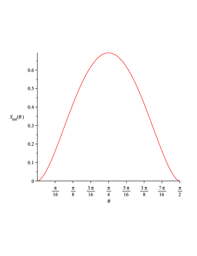
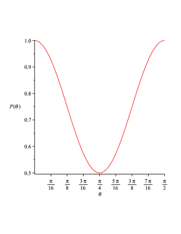
Figure 1: Entanglement entropy $S_{\rm ent}$ and purity $P$ versus parameter $\theta$ where $\cos\theta=\lambda^{(1)}_{1}$. The conventional ordering $\lambda^{(1)}_{1}\geq\lambda^{(1)}_{2}$ corresponds to $0\leq\theta\leq\frac{\pi}{4}$.

$\bullet$  In the case of $\lambda^{(1)}_{1}=\lambda^{(1)}_{2}$, from (36) and (41) we have $\lambda^{(2)}_{1}=\lambda^{(2)}_{2}$ since otherwise, i.e. for $\lambda^{(2)}_{1}\neq\lambda^{(2)}_{2}$, in view of (41) we have $\mathop{\mathrm{Tr}}\nolimits(D_{1}\tilde{\Phi}^{\dagger}_{2})=e^{-i\eta}\lambda^{(1)}_{1}\bigl{(}\lambda^{(2)}_{1}\frac{\overline{\tilde{u}_{1}}}{\overline{\tilde{v}_{1}}}+\lambda^{(2)}_{2}\frac{\tilde{u}_{1}}{\tilde{v}_{1}}\bigr{)}\neq 0$ that contradicts (36). In this case according to (35) we have

$$\tilde{\Phi}_{2}=e^{i\eta}\lambda^{(2)}_{1}\tilde{U},\quad\mathop{\mathrm{Tr}}\nolimits\tilde{U}=0,$$

and the respective Schmidt coefficient squared $(\lambda^{(\alpha)}_{i})^{2}$, $\alpha,i=\overline{1,2}$, is equal to $1/2$. So, the entanglement entropy within the composite fermion in each of the two modes $\alpha=1$ or $2$ is $S_{\rm ent}=\ln 2$, that is the constant which coincides with maximal value for the case of (42).

5 Composite fermions as composites of fermion and deformed boson: two-mode case

Let us go over to the two-mode case ($\alpha=1,\,2$) of CF when it is composed of usual fermion and, say, $\chi$-deformed boson. In this case the specifics of two modes for the CFs implies that it is again sufficient to consider realization conditions (11)-(13) on the vacuum and one-CF states. Indeed, for single non-zero two-CF state $A_{1}^{\dagger}A_{2}^{\dagger}|0\rangle$, implying that realization conditions  (11)-(13) hold on the vacuum and one-CF states, we have

$$(A_{1}^{\dagger}A_{1}-\varphi(N_{1}))A_{1}^{\dagger}A_{2}^{\dagger}|0\rangle=-A_{2}^{\dagger}(A_{1}^{\dagger}A_{1}-\varphi(N_{1}))A_{1}^{\dagger}|0\rangle=0;$$

$$(A_{1}A_{1}^{\dagger}-\varphi(N_{1}+1))A_{1}^{\dagger}A_{2}^{\dagger}|0\rangle=A_{2}^{\dagger}\varphi(N_{1}+1)A_{1}^{\dagger}|0\rangle=0;$$

$$\{A_{1},A_{2}^{\dagger}\}A_{1}^{\dagger}A_{2}^{\dagger}|0\rangle=A_{2}^{\dagger}A_{1}A_{1}^{\dagger}A_{2}^{\dagger}|0\rangle=(A_{2}^{\dagger})^{2}A_{1}A_{1}^{\dagger}|0\rangle=0.$$

The corresponding (to one-CF states) realization condition (24) then reduces to the following two independent equations (denote $\delta\chi_{2}\equiv\chi(2)\!-\!2$):

$$\Phi_{1}\Phi_{1}^{\dagger}\Phi_{2}-\Phi_{2}\Phi_{1}^{\dagger}\Phi_{1}+\delta\chi_{2}\bigl{[}\mathop{\mathrm{diag}}\nolimits\{(\Phi_{1}\Phi_{1}^{\dagger})^{\mu\mu}\}\Phi_{2}-\mathop{\mathrm{diag}}\nolimits\{(\Phi_{2}\Phi_{1}^{\dagger})^{\mu\mu}\}\Phi_{1}\bigr{]}=0,$$ (45)

$$\Phi_{1}\Phi_{2}^{\dagger}\Phi_{2}-\Phi_{2}\Phi_{2}^{\dagger}\Phi_{1}+\delta\chi_{2}\bigl{[}\mathop{\mathrm{diag}}\nolimits\{(\Phi_{1}\Phi_{2}^{\dagger})^{\mu\mu}\}\Phi_{2}-\mathop{\mathrm{diag}}\nolimits\{(\Phi_{2}\Phi_{2}^{\dagger})^{\mu\mu}\}\Phi_{1}\bigr{]}=0.$$ (46)

Performing the replacement (30) as in the case of non-deformed constituent boson we arrive at the following system of equations equivalent to (45), (46), but now given in terms of $D_{1}$ and $\tilde{\Phi}_{2}$:

$$D_{1}^{2}\tilde{\Phi}_{2}-\tilde{\Phi}_{2}D_{1}^{2}+\delta\chi_{2}\bigl{[}U_{1}^{\dagger}\mathop{\mathrm{diag}}\nolimits\{(U_{1}D_{1}^{2}U_{1}^{\dagger})^{\mu\mu}\}U_{1}\tilde{\Phi}_{2}-U_{1}^{\dagger}\mathop{\mathrm{diag}}\nolimits\{(U_{1}\tilde{\Phi}_{2}D_{1}U_{1}^{\dagger})^{\mu\mu}\}U_{1}D_{1}\bigr{]}=0,$$ (47)

$$D_{1}\tilde{\Phi}_{2}^{\dagger}\tilde{\Phi}_{2}-\tilde{\Phi}_{2}\tilde{\Phi}_{2}^{\dagger}D_{1}+\delta\chi_{2}\bigl{[}U_{1}^{\dagger}\mathop{\mathrm{diag}}\nolimits\{(U_{1}D_{1}\tilde{\Phi}_{2}^{\dagger}U_{1}^{\dagger})^{\mu\mu}\}U_{1}\tilde{\Phi}_{2}-U_{1}^{\dagger}\mathop{\mathrm{diag}}\nolimits\{(U_{1}\tilde{\Phi}_{2}\tilde{\Phi}_{2}^{\dagger}U_{1}^{\dagger})^{\mu\mu}\}U_{1}D_{1}\bigr{]}=0.$$ (48)

To find the Schmidt coefficients $\lambda^{\alpha}_{i}$, $\alpha=1,\,2$, contained in the definition of entanglement entropy it may be convenient to deal with the variables $X_{\alpha}=\Phi_{\alpha}\Phi_{\alpha}^{\dagger}$, $Y=\Phi_{2}\Phi_{1}^{\dagger}$, since $|\lambda^{\alpha}_{i}|^{2}$ are the eigenvalues of $X_{\alpha}$. Multiplying (45) and (46) y $\Phi_{1}$ from the right we obtain the equations

$$X_{1}Y-YX_{1}+\delta\chi_{2}[\mathop{\mathrm{diag}}\nolimits\{X_{1}^{\mu\mu}\}Y-\mathop{\mathrm{diag}}\nolimits\{Y^{\mu\mu}\}X_{1}]=0,$$

$$Y^{\dagger}Y-X_{2}X_{1}+\delta\chi_{2}[\mathop{\mathrm{diag}}\nolimits\{\overline{Y^{\mu\mu}}\}Y-\mathop{\mathrm{diag}}\nolimits\{X_{2}^{\mu\mu}\}X_{1}]=0$$

which for nondegenerate $\Phi_{1}$ are equivalent to (45), (46).

Restricting ourselves to the case of two modes $\mu,\nu=1,\,2$ of the constituents, without loss of generality we take $U_{1}\in SU(2)$. Using the parametrization: $U_{1}=\Bigl{(}\begin{array}[]{cc}u&v\\ -\overline{v}&\overline{u}\end{array}\Bigr{)}$, $|u|^{2}+|v|^{2}=1$, and the identity

$$U_{1}^{\dagger}\mathop{\mathrm{diag}}\nolimits\{(U_{1}XU_{1}^{\dagger})^{\mu\mu}\}U_{1}=\frac{1}{2}X+\frac{1}{2}RXR,\quad R=\Bigl{(}\begin{array}[]{cc}|u|^{2}\!-\!|v|^{2}&2\overline{u}v\\ 2u\overline{v}&|v|^{2}\!-\!|u|^{2}\end{array}\Bigr{)},$$ (49)

we rewrite equations (47) and (48) respectively as

$$\frac{\chi(2)}{2}(D_{1}^{2}\tilde{\Phi}_{2}-\tilde{\Phi}_{2}D_{1}^{2})+\frac{\delta\chi_{2}}{2}\bigl{(}RD_{1}^{2}R\tilde{\Phi}_{2}-R\tilde{\Phi}_{2}D_{1}RD_{1}\bigr{)}=0,$$ (50)

$$\frac{\chi(2)}{2}(D_{1}\tilde{\Phi}_{2}^{\dagger}\tilde{\Phi}_{2}-\tilde{\Phi}_{2}\tilde{\Phi}_{2}^{\dagger}D_{1})+\frac{\delta\chi_{2}}{2}\bigl{(}RD_{1}\tilde{\Phi}_{2}^{\dagger}R\tilde{\Phi}_{2}-R\tilde{\Phi}_{2}\tilde{\Phi}_{2}^{\dagger}RD_{1}\bigr{)}=0.$$ (51)

Taking into account three-dimensionality of the subspace of matrices $\tilde{\Phi}^{\dagger}_{2}$ satisfying the orthogonality condition $\mathop{\mathrm{Tr}}\nolimits(D_{1}\tilde{\Phi}^{\dagger}_{2})=0$ we look for the solution of (50)-(51) as the linear combination of the following basis elements:

$$\tilde{\Phi}_{2}=x_{1}\Bigl{(}\begin{array}[]{cc}\lambda^{(1)}_{2}&0\\ 0&-\lambda^{(1)}_{1}\end{array}\Bigr{)}+x_{2}\Bigl{(}\begin{array}[]{cc}0&\varkappa\lambda^{(1)}_{1}\\ \overline{\varkappa}\lambda^{(1)}_{2}&0\end{array}\Bigr{)}+x_{3}\Bigl{(}\begin{array}[]{cc}0&-\varkappa\lambda^{(1)}_{2}\\ \overline{\varkappa}\lambda^{(1)}_{1}&0\end{array}\Bigr{)},\ \ \ \varkappa=e^{i(\arg v-\arg u)}.$$ (52)

Then, after some calculation equation (50) reduces to the system of linear (in $x_{1},x_{2},x_{3}$) equations

$$2\delta\chi_{2}|u|^{2}|v|^{2}x_{1}-\delta\chi_{2}|u||v|(|u|^{2}-|v|^{2})x_{2}=0,$$ (53)

$$-\delta\chi_{2}|u||v|(|u|^{2}\!-\!|v|^{2})x_{1}\!+\!\frac{1}{2}\bigl{(}\chi(2)((\lambda^{(1)}_{1})^{2}\!-\!(\lambda^{(1)}_{2})^{2})^{2}\!+\!\delta\chi_{2}(|u|^{2}\!-\!|v|^{2})^{2}\bigr{)}x_{2}+$$

$$\hskip 56.9055pt+\chi(2)\lambda^{(1)}_{1}\lambda^{(1)}_{2}((\lambda^{(1)}_{2})^{2}\!-\!(\lambda^{(1)}_{1})^{2})x_{3}\!=\!0,$$ (54)

$$\chi(2)\lambda^{(1)}_{1}\lambda^{(1)}_{2}((\lambda^{(1)}_{2})^{2}-(\lambda^{(1)}_{1})^{2})x_{2}-\frac{1}{2}\bigl{(}\chi(2)((\lambda^{(1)}_{1})^{2}-(\lambda^{(1)}_{2})^{2})^{2}-\delta\chi_{2}\bigr{)}x_{3}=0.$$ (55)

For the existence of a nontrivial solution, the determinant of this system should be zero, i.e.

$$\det\bigl{(}...\bigr{)}=-\chi(2)(\chi(2)-2)|u|^{2}|v|^{2}((\lambda^{(1)}_{1})^{2}-(\lambda^{(1)}_{2})^{2})^{2}=0.$$

That is possible in the following cases:

a) $\chi(2)=2$. Then eqs. (47), (48) reduce to non-deformed eqs. (32), (33) which were already considered.

b) $\chi(2)=0$ or $\lambda^{(1)}_{1}=\lambda^{(1)}_{2}$ at $\chi(2)\neq 2$. Though the situation $\lambda^{(1)}_{1}=\lambda^{(1)}_{2}$ is qualitatively different, in this case the solution of (53)-(55) is given uniformly, namely

$$\tilde{\Phi}_{2}=\kappa R\left(\begin{array}[]{cc}\lambda^{(1)}_{2}&0\\ 0&\lambda^{(1)}_{1}\end{array}\right),\quad|\kappa|=1,\ \ (\lambda^{(1)}_{1})^{2}+(\lambda^{(1)}_{2})^{2}=1,$$ (56)

yielding the entanglement entropy

$$S_{\rm ent}|_{\alpha=1,2}=-(\lambda^{(1)}_{1})^{2}\ln(\lambda^{(1)}_{1})^{2}-(1-(\lambda^{(1)}_{1})^{2})\ln(1-(\lambda^{(1)}_{1})^{2})\ =S_{2}(\theta),\quad 0\leq\theta\leq\frac{\pi}{4}$$ (57)

(to be compared with (42)-(43)) which for $\lambda^{(1)}_{1}=\lambda^{(1)}_{2}=\frac{1}{\sqrt{2}}$ yields $S_{\rm ent}|_{\alpha=1,2}=\ln 2$.

c) $uv=0$ while $\chi(2)$ is unrestricted, and $\lambda^{(1)}_{1}\neq\lambda^{(1)}_{2}$. Equation (50) takes the form

$$\bigl{(}\chi(2)(\lambda^{(1)}_{1})^{2}-1\bigr{)}\phi^{(2)}_{12}=0,\quad\bigl{(}\chi(2)(\lambda^{(1)}_{2})^{2}-1\bigr{)}\phi^{(2)}_{21}=0.$$

Eq. (51) e.g. with $\phi^{(2)}_{21}=0$ reduces to

$$\left(\begin{array}[]{cc}-(\chi(2)-1)\lambda^{(1)}_{1}|\phi^{(2)}_{12}|^{2}&\frac{1}{2}\chi(2)(\lambda^{(1)}_{1}\overline{\phi^{(2)}_{11}}-\lambda^{(1)}_{2}\overline{\phi^{(2)}_{22}})\phi^{(2)}_{12}\\ (\lambda^{(1)}_{2}\phi^{(2)}_{11}-\lambda^{(1)}_{1}\phi^{(2)}_{22})\overline{\phi^{(2)}_{12}}&\lambda^{(1)}_{2}|\phi^{(2)}_{12}|^{2}\end{array}\right)=0.$$

So, there are two solutions:

• $\tilde{\Phi}_{2}=\kappa\mathop{\mathrm{diag}}\nolimits\bigl{\{}\lambda^{(1)}_{2},-\lambda^{(1)}_{1}\bigr{\}}$, $(\lambda^{(1)}_{1})^{2}+(\lambda^{(1)}_{2})^{2}=1$, $|\kappa|=1$, so that   $S_{\rm ent}|_{\alpha=1,2}=S_{2}(\theta)$, $\lambda^{(1)}_{1}=\cos\theta$, $0\leq\theta\leq\frac{\pi}{4}$. Note, this result coincides with (57), see also eq. (42) and Fig. 1.

• If $\chi(2)=1$, there appears the additional solution $\tilde{\Phi}_{2}=\left(\begin{array}[]{cc}0&\phi^{(2)}_{12}\\ 0&0\end{array}\right)$, $|\phi^{(2)}_{12}|=1$, $\lambda^{(1)}_{1}=1$, $\lambda^{(1)}_{2}=0$, so that $S_{\rm ent}=0$;

To summarize: the entanglement entropy of the composite fermion is either constant $S_{\rm ent}=\ln 2$ or $S_{\rm ent}=0$ in some special cases, or it is given by a general parameter-dependent expression, see (57). Let us also remark on the effect of the deformation parameter, say through $\chi(2)$. Though for each of the considered cases it has not entered the resp. Schmidt coefficients and entanglement entropy, it can manifest itself when calculating the averages of physical quantities over quantum states.

6 More general situations for composite fermions built from fermion and deformed boson

Before we proceed further examples generalizing the above ones, let us make some general remark. Denoting by $D_{CF}$ and $D_{f}$ the number of modes respectively for composite fermions and the constituent fermions, we have: $D_{CF}\leq D_{f}$. Indeed, let $(\alpha_{1},...,\alpha_{D_{CF}})$ be the set of all (differing) CF modes, and let $D_{CF}>D_{f}$. Now evaluate the state

$$A_{\alpha_{1}}A_{\alpha_{1}}^{\dagger}A_{\alpha_{2}}^{\dagger}...A_{\alpha_{D_{CF}}}^{\dagger}|0\rangle=\sum_{\mu\nu...\mu_{D_{CF}}\nu_{D_{CF}}}\overline{\Phi_{\alpha_{1}}^{\mu\nu}}\Phi_{\alpha_{1}}^{\mu\nu}...\Phi_{\alpha_{D_{CF}}}^{\mu_{D_{CF}}\nu_{D_{CF}}}a_{\mu}b_{\nu}a^{\dagger}_{\mu_{1}}b^{\dagger}_{\nu_{1}}...a^{\dagger}_{\mu_{D_{CF}}}b^{\dagger}_{\nu_{D_{CF}}}|0\rangle=0.$$ (58)

Since among $b^{\dagger}_{\nu_{1}}$,…,$b^{\dagger}_{\nu_{D_{CF}}}$, for $D_{CF}>D_{f}$, there are at least two coinciding fermionic creation operators, that results in zero. On the other hand, using realization conditions (11)-(13) we have

$$A_{\alpha_{1}}A_{\alpha_{1}}^{\dagger}A_{\alpha_{2}}^{\dagger}...A_{\alpha_{D_{CF}}}^{\dagger}|0\rangle=A_{\alpha_{2}}^{\dagger}...A_{\alpha_{D_{CF}}}^{\dagger}|0\rangle\neq 0.$$

The latter inequality holds due to the orthonormality and mode-independence conditions for (deformed) fermions which realize CFs, see (19), (12), (15). But that contradicts (58). So we conclude that $D_{CF}\leq D_{f}$. Then, as further directions of the extension of the considered $D_{CF}=D_{f}=D_{b}=2$ case where $D_{b}$ is the number of modes for the (non-deformed or deformed) constituent boson, such cases that $D_{CF}=2$, $D_{f}=D_{b}=3$, and $D_{CF}=3$, $D_{f}=3$ can also be treated.

Composite fermions in two modes, with non-deformed constituents in three modes.

In this case we take $\alpha=\overline{1,2}$, $\mu,\nu=\overline{1,3}$ so that $\Phi_{\alpha}^{\mu\nu}$ are some two $3\times 3$-matrices. The realization conditions retain the form (31)-(33). Writing $D_{1}$ and $\tilde{\Phi}_{2}$ explicitly as

$$D_{1}=\mathop{\mathrm{diag}}\nolimits\{\lambda^{(1)}_{1},\lambda^{(1)}_{2},\lambda^{(1)}_{3}\},\quad\tilde{\Phi}_{2}=\left(\begin{array}[]{ccc}\phi_{11}&\phi_{12}&\phi_{13}\\ \phi_{21}&\phi_{22}&\phi_{23}\\ \phi_{31}&\phi_{32}&\phi_{33}\end{array}\right),$$ (59)

eq. (32) yields the system

$$((\lambda^{(1)}_{i})^{2}-(\lambda^{(1)}_{j})^{2})\phi_{ij}=0,\quad i\neq j,\ \ 1\leq i,j\leq 3.$$ (60)

If the diagonal elements of $D_{1}$ are different, $\lambda^{(1)}_{i}\neq\lambda^{(1)}_{j}$, $i\neq j$, then $\phi_{ij}=0$ for $i\neq j$, i.e. matrix $\tilde{\Phi}_{2}$ is diagonal too: $\tilde{\Phi}_{2}=\mathop{\mathrm{diag}}\nolimits\{\phi_{11},\phi_{22},\phi_{33}\}$, $|\phi_{11}|^{2}+|\phi_{22}|^{2}+|\phi_{33}|^{2}=1$. The only remaining nontrivial realization condition is the orthogonality condition in (31), which reduces to the orthogonality condition for the vectors $(\lambda^{(1)}_{1},\lambda^{(1)}_{2},\lambda^{(1)}_{3})$ and $(\phi_{11},\phi_{22},\phi_{33})$, i.e.

$$\lambda^{(1)}_{1}\overline{\phi_{11}}+\lambda^{(1)}_{2}\overline{\phi_{22}}+\lambda^{(1)}_{3}\overline{\phi_{33}}=0.$$ (61)

For the entanglement entropy within a CF belonging to each of the two modes we have

$$S_{\rm ent}^{(1)}\equiv S_{\rm ent}|_{\alpha=1}=-\sum_{i=1}^{3}(\lambda^{(1)}_{i})^{2}\ln(\lambda^{(1)}_{i})^{2},\quad S_{\rm ent}^{(2)}\equiv S_{\rm ent}|_{\alpha=2}=-\sum_{i=1}^{3}|\phi_{ii}|^{2}\ln|\phi_{ii}|^{2}.$$ (62)

It can be parameterized by the angles e.g. in the form

$$\lambda^{(1)}_{1}=\cos\theta^{(1)}_{1}\cos\theta^{(1)}_{2},\quad\lambda^{(1)}_{2}=\cos\theta_{1}^{(1)}\sin\theta_{2}^{(1)},\quad\lambda^{(1)}_{3}=\sin\theta_{1}^{(1)},$$ (63)

$$|\phi_{11}|=\cos\theta_{1}^{(2)}\cos\theta_{2}^{(2)},\quad|\phi_{22}|=\cos\theta_{1}^{(2)}\sin\theta_{2}^{(2)},\quad|\phi_{33}|=\sin\theta_{1}^{(2)}.$$ (64)

Then the condition (61) gives the following relation between the angles:

$$\cos^{2}\theta_{1}^{(2)}=\frac{\sin^{2}\theta_{1}^{(1)}}{1-\sin^{2}\Omega\cos^{2}\theta_{1}^{(1)}}$$ (65)

where the angle $\Omega$ is defined as $\cos 2\Omega\equiv\cos 2\theta_{2}^{(1)}\cos 2\theta_{2}^{(2)}+\sin 2\theta_{2}^{(1)}\sin 2\theta_{2}^{(2)}\cos\gamma^{\prime}$ with $\gamma^{\prime}\equiv\arg(d_{1}\overline{d_{2}}\overline{\phi_{11}}\phi_{22})$, and belonging to the interval $|\theta_{2}^{(1)}-\theta_{2}^{(2)}|<\Omega<\theta_{2}^{(1)}+\theta_{2}^{(2)}$. Substituting (63) and (64) in (62) and using (65), we obtain

$$S_{\rm ent}^{(1)}=S_{2}(\theta_{1}^{(1)})+\cos^{2}\theta_{1}^{(1)}S_{2}(\theta_{2}^{(1)}),$$ (66)

$$S_{\rm ent}^{(2)}=\frac{S_{2}(\theta_{2}^{(2)})-\mathop{\mathrm{ctg}}\nolimits^{2}\theta_{1}^{(1)}\cos^{2}\Omega\,\ln(\mathop{\mathrm{ctg}}\nolimits^{2}\theta_{1}^{(1)}\cos^{2}\Omega)}{1+\mathop{\mathrm{ctg}}\nolimits^{2}\theta_{1}^{(1)}\cos^{2}\Omega}+\ln(1+\mathop{\mathrm{ctg}}\nolimits^{2}\theta_{1}^{(1)}\cos^{2}\Omega)$$ (67)

where the function $S_{2}(x)$ is defined in (43).

Remark. Another parametrization of two orthonormal vectors $(\lambda^{(1)}_{1},\lambda^{(1)}_{2},\lambda^{(1)}_{3})$ and $(\phi_{11},\phi_{22},\phi_{33})$ follows from the parametrization of $SU(3)$ since the rows/colums of matrices from $SU(3)$ constitute orthonormal vectors. Indeed, using the parametrization given in [27] and retaining the parametrization (63) for $\alpha=1$ mode we have the following parametrization for the $\alpha=2$ mode ($\theta_{1,2}\equiv\theta_{1,2}^{(1)}$):

$$\phi_{11}=-\sin\theta_{1}\cos\theta_{2}\cos\theta_{3}-\sin\theta_{2}\sin\theta_{3}e^{i\gamma},\quad\phi_{22}=\cos\theta_{2}\sin\theta_{3}e^{i\gamma}-\sin\theta_{1}\sin\theta_{2}\cos\theta_{3},$$

$$\phi_{33}=\cos\theta_{1}\cos\theta_{3},\qquad 0\leq\theta_{1},\theta_{2},\theta_{3}\leq\pi/2,\ \ 0\leq\gamma\leq 2\pi.$$ (68)

The corresponding entanglement entropy expressions, $S_{\rm ent}^{(1)}(\theta_{1},\theta_{2})$ and $S_{\rm ent}^{(2)}(\theta_{1},\theta_{2},\theta_{3},\gamma)$, stem from (62). To achieve standard ordering $\lambda^{(1)}_{1}\geq\lambda^{(1)}_{2}\geq\lambda^{(1)}_{3}$ we have to impose $0\leq\theta_{2}\leq\frac{\pi}{4}$, $0\leq\theta_{1}\leq\mathop{\mathrm{arctg}}\nolimits\sin\theta_{2}$.

Thus, composite fermion entanglement entropies $S_{\rm ent}^{(1)}$, $S_{\rm ent}^{(2)}$ in eq. (62) are parameterized by four angles. Unlike the two-mode $\mu,\nu=\overline{1,2}$ case considered in Section 4 where $S_{\rm ent}^{(1)}-S_{\rm ent}^{(2)}=0$, and $0\leq S_{\rm ent}^{(\alpha)}\leq\ln 2$, $\alpha=\overline{1,2}$, now it can be shown for the $\mu,\nu=\overline{1,3}$ case that $|S_{\rm ent}^{(1)}-S_{\rm ent}^{(2)}|\leq\ln 2$, and $0\leq S_{\rm ent}^{(\alpha)}\leq\ln 3$. This restriction on the difference $|S_{\rm ent}^{(1)}-S_{\rm ent}^{(2)}|$ can be viewed as the necessary condition for the realization. For the illustration of the dependence $S_{\rm ent}^{(\alpha)}=S_{\rm ent}^{(\alpha)}(\theta_{1}^{(\alpha)},\theta_{2}^{(\alpha)})$ at a fixed mode $\alpha$ with the other one ignored, equi-entropic curves in the resp. $\theta_{1}$-, $\theta_{2}$-angles are given in Fig. 2 (left). A similar behavior can be seen e.g. in [28], in the context of the $SU(3)$ parametrization of qutrits.

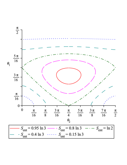
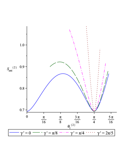
Figure 2: Left: Equi-entropic curves (for constant composite fermion entanglement entropy $S_{\rm ent}^{(\alpha)}$) versus parameters $\theta_{1}^{(\alpha)},\theta_{2}^{(\alpha)}$, at a fixed mode $\alpha=1$ or $2$ (the case of three-mode constituents). Right: Entanglement entropy $S_{\rm ent}^{(2)}(\theta_{1}^{(2)},\gamma^{\prime})$ for a composite fermion in $\alpha=2$ mode at fixed entanglement entropy $S_{\rm ent}^{(1)}=\ln 3$ for $\alpha=1$ mode of composite fermion.

Let us consider the case when two diagonal elements of $D_{1}$, e.g. $\lambda^{(1)}_{1}$ and $\lambda^{(1)}_{2}$ coincide, but differ from the remaining one: $\lambda^{(1)}_{1}=\lambda^{(1)}_{2}\neq\lambda^{(1)}_{3}$. Condition (60) yields $\phi_{13}=\phi_{23}=\phi_{31}=\phi_{32}=0$. Next, we present the $2\times 2$ block $\Bigl{(}{\scriptstyle\phi_{11}\ \phi_{12}\atop\scriptstyle\phi_{21}\ \phi_{22}}\Bigr{)}$ of $\tilde{\Phi}_{2}$ using singular value decomposition applied for $SU(2)$-matrices,

$$\left(\begin{array}[]{cc}\phi_{11}&\phi_{12}\\ \phi_{21}&\phi_{22}\end{array}\right)=e^{i\eta}\tilde{U}\tilde{D}_{2}\tilde{V}^{\dagger}=e^{i\eta}\left(\begin{array}[]{cc}\tilde{u}_{1}&\tilde{u}_{2}\\ -\overline{\tilde{u}_{2}}&\overline{\tilde{u}_{1}}\end{array}\right)\left(\begin{array}[]{cc}\lambda^{(2)}_{1}&0\\ 0&\lambda^{(2)}_{2}\end{array}\right)\left(\begin{array}[]{cc}\tilde{v}_{1}&\tilde{v}_{2}\\ -\overline{\tilde{v}_{2}}&\overline{\tilde{v}_{1}}\end{array}\right)^{\dagger}$$ (69)

where the three matrices $\tilde{U}$, $\tilde{D}_{2}$, and $\tilde{V}$ are shown explicitly. Then (33) (at $\lambda^{(1)}_{1}=\lambda^{(1)}_{2}\neq 0$) reduces to the equations as in (41). The orthogonality condition in (31) then yields

$$\lambda^{(1)}_{1}\lambda^{(2)}_{1}(\tilde{u}_{1}\overline{\tilde{v}_{1}}+\overline{\tilde{u}_{2}}\tilde{v}_{2})+\lambda^{(1)}_{1}\lambda^{(2)}_{2}(\overline{\tilde{u}_{1}}\tilde{v}_{1}+\tilde{u}_{2}\overline{\tilde{v}_{2}})=-e^{-i\eta}\lambda^{(1)}_{3}\phi_{33}.$$

$\bullet$  If $\lambda^{(2)}_{1}=\lambda^{(2)}_{2}$, eqs. from (41) are satisfied while the block (69) is proportional to a unitary matrix,

$$\left(\begin{array}[]{cc}\phi_{11}&\phi_{12}\\ \phi_{21}&\phi_{22}\end{array}\right)\biggr{|}_{\lambda^{(2)}_{1}=\lambda^{(2)}_{2}}=\lambda^{(2)}_{1}e^{i\eta}U^{\prime},\quad U^{\prime}=\left(\begin{array}[]{cc}u^{\prime}_{1}&u^{\prime}_{2}\\ -\overline{u^{\prime}_{2}}&\overline{u^{\prime}_{1}}\end{array}\right)\in SU(2),$$

that leads to the orthogonality condition

$$\lambda^{(1)}_{1}\lambda^{(2)}_{1}e^{i\eta}(u^{\prime}_{1}+\overline{u^{\prime}_{1}})\!=\!-\lambda^{(1)}_{3}\phi_{33}\ \Rightarrow\ 2\lambda^{(2)}_{1}\lambda^{(1)}_{1}|{\rm Re}\,u^{\prime}_{1}|\!=\!\sqrt{1\!-\!2(\lambda^{(1)}_{1})^{2}}\sqrt{1\!-\!2(\lambda^{(2)}_{1})^{2}}.$$

The solution for $\Phi_{1}$ and $\Phi_{2}$ is then written as

$$\Phi_{1}=U_{1}\mathop{\mathrm{diag}}\nolimits\{\lambda^{(1)}_{1},\lambda^{(1)}_{2},\lambda^{(1)}_{3}\}V_{1}=\tilde{U}_{1}\left(\begin{array}[]{cc}\lambda^{(1)}_{1}e^{i\gamma_{d}}(U^{\prime\prime})^{\dagger}&0\\ 0&\lambda^{(1)}_{3}\end{array}\right)V_{1},$$ (70)

$$\Phi_{2}=U_{1}\left(\begin{array}[]{cc}\lambda^{(2)}_{1}e^{i\eta}U^{\prime}&0\\ 0&\phi_{33}\end{array}\right)V_{1}=\tilde{U}_{1}\left(\begin{array}[]{cc}\lambda^{(2)}_{1}e^{i\eta}U^{\prime\prime}&0\\ 0&\phi_{33}\end{array}\right)V_{1},$$

where

$$\tilde{U}_{1}=U_{1}\left(\begin{array}[]{cc}U_{d}U^{\prime\prime}&0\\ 0&1\end{array}\right),\ \ \ \left(\begin{array}[]{cc}\lambda^{(1)}_{1}&0\\ 0&\lambda^{(1)}_{2}\end{array}\right)\equiv\lambda^{(1)}_{1}e^{i\gamma_{d}}U_{d},\ \ \ U_{d}^{\dagger}U^{\prime}=(U^{\prime\prime})^{2},\ \ U_{d},U^{\prime\prime}\in SU(2).$$

For the entanglement entropy of composite fermion in this subcase we find

$$S_{\rm ent}^{(1)}=-\cos^{2}\theta_{1}\ln\Bigl{(}\frac{1}{2}\cos^{2}\theta_{1}\Bigr{)}-\sin^{2}\theta_{1}\ln\sin^{2}\theta_{1}=\cos^{2}\theta_{1}\ln 2+S_{2}(\theta_{1}),$$ (71)

$$S_{\rm ent}^{(2)}=\ln\Bigl{(}\mathop{\mathrm{tg}}\nolimits^{2}\theta_{1}\!+\!\frac{1}{4}|\mathop{\mathrm{Tr}}\nolimits U^{\prime}|^{2}\Bigr{)}-\frac{\mathop{\mathrm{tg}}\nolimits^{2}\theta_{1}\ln\bigl{(}\frac{1}{2}\mathop{\mathrm{tg}}\nolimits^{2}\theta_{1}\bigr{)}\!+\!\frac{1}{4}|\mathop{\mathrm{Tr}}\nolimits U^{\prime}|^{2}\ln\bigl{(}\frac{1}{4}|\mathop{\mathrm{Tr}}\nolimits U^{\prime}|^{2}\bigr{)}}{\mathop{\mathrm{tg}}\nolimits^{2}\theta_{1}+\frac{1}{4}|\mathop{\mathrm{Tr}}\nolimits U^{\prime}|^{2}},\ \ \ 0\leq|\mathop{\mathrm{Tr}}\nolimits U^{\prime}|\leq 2.$$ (72)

$\bullet$  If $\lambda^{(2)}_{1}\neq\lambda^{(2)}_{2}$, from eqs. in (41) we obtain

$$\lambda^{(1)}_{1}(|u_{1}|-|v_{1}|)=0;\quad\lambda^{(1)}_{1}(\tilde{u}_{1}\tilde{u}_{2}-\tilde{v}_{1}\tilde{v}_{2})=0\ \ \mathop{\Rightarrow}\limits_{\lambda^{(1)}_{1}\neq 0}\ \ \lambda^{(1)}_{1}\lambda^{(2)}_{1}\frac{\tilde{u}_{1}}{\tilde{v}_{1}}+\lambda^{(1)}_{1}\lambda^{(2)}_{2}\frac{\overline{\tilde{u}_{1}}}{\overline{\tilde{v}_{1}}}=-e^{-i\eta}\lambda^{(1)}_{3}\phi_{33}.$$

Let $\frac{\tilde{u}_{1}}{\tilde{v}_{1}}=e^{i\delta}$. Then $\tilde{V}=\tilde{U}\mathop{\mathrm{diag}}\nolimits\{e^{-i\delta},e^{i\delta}\}$ and the involved parameters are related as

$$\lambda^{(1)}_{1}|\lambda^{(2)}_{1}e^{i\delta}+\lambda^{(2)}_{2}e^{-i\delta}|=\sqrt{1\!-\!2(\lambda^{(1)}_{1})^{2}}\sqrt{1\!-\!(\lambda^{(2)}_{1})^{2}\!-\!(\lambda^{(2)}_{2})^{2}}.$$ (73)

The corresponding expression for the entanglement entropy $S_{\rm ent}^{(2)}$ for the $\alpha=2$ mode reads

$$S_{\rm ent}^{(2)}=\ln 2-|\sin\theta_{1}\cos\theta_{3}+\sin\theta_{3}e^{i\gamma}|^{2}\ln|\sin\theta_{1}\cos\theta_{3}+\sin\theta_{3}e^{i\gamma}|-\\ -|\sin\theta_{1}\cos\theta_{3}-\sin\theta_{3}e^{i\gamma}|^{2}\ln|\sin\theta_{1}\cos\theta_{3}-\sin\theta_{3}e^{i\gamma}|-\cos^{2}\theta_{1}\cos^{2}\theta_{3}\ln(2\cos^{2}\theta_{1}\cos^{2}\theta_{3}),$$ (74)

while $S_{\rm ent}^{(1)}$ is given in (71).

For the case $\lambda^{(1)}_{1}=\lambda^{(1)}_{2}=\lambda^{(1)}_{3}$ matrix $\tilde{\Phi}_{2}$ satisfies relations (34). Presenting $\tilde{\Phi}_{2}$ as in (35) with $D_{2}=\mathop{\mathrm{diag}}\nolimits\{\lambda^{(2)}_{1},\lambda^{(2)}_{2},\lambda^{(2)}_{3}\}$, $\tilde{U},\tilde{V}\in SU(3)$, we obtain the equations similar to (31), (32):

$$D_{2}^{2}W=WD_{2}^{2},\quad\mathop{\mathrm{Tr}}\nolimits(D_{2}W)=0,\quad\mathop{\mathrm{Tr}}\nolimits D_{2}^{2}=1,\quad W=\tilde{V}^{\dagger}\tilde{U}\in SU(3).$$ (75)

If $\lambda^{(2)}_{i}\neq\lambda^{(2)}_{j}$, $i\neq j$, from equation analogous to (60) we have the solution

$$W=\mathop{\mathrm{diag}}\nolimits\{w_{11},w_{22},w_{33}\},\quad|w_{ii}|=1,\ \ i=\overline{1,3},\quad\sum\nolimits_{i}\lambda^{(2)}_{i}w_{ii}=0,$$ (76)

so that $\tilde{\Phi}_{2}=e^{i\eta}\tilde{U}\,D_{2}W\,\tilde{U}^{\dagger}$. If $\lambda^{(2)}_{1}\!=\!\lambda^{(2)}_{2}\!\neq\!\lambda^{(2)}_{3}$, matrix $W$ is block-diagonal, $W=\mathop{\mathrm{diag}}\nolimits\{w_{33}^{-1/2}W^{\prime},w_{33}\}$, $|w_{33}|=1$, $W^{\prime}\in SU(2)$. From the second equation in (75) we have

$$\lambda^{(2)}_{1}w_{33}^{-1/2}\mathop{\mathrm{Tr}}\nolimits W^{\prime}+\lambda^{(2)}_{3}w_{33}=0\quad\Rightarrow\quad\lambda^{(2)}_{3}=|\mathop{\mathrm{Tr}}\nolimits W^{\prime}|\lambda^{(2)}_{1},\ \ \ 0\leq|\mathop{\mathrm{Tr}}\nolimits W^{\prime}|\leq 2,$$

so that $\tilde{\Phi}_{2}=e^{i\eta}\tilde{U}\mathop{\mathrm{diag}}\nolimits\{w_{33}^{-1/2}\lambda^{(2)}_{1}W^{\prime},w_{33}\lambda^{(2)}_{3}\}\tilde{U}^{\dagger}$. If $\lambda^{(2)}_{1}\!=\!\lambda^{(2)}_{2}\!=\!\lambda^{(2)}_{3}$: $\tilde{\Phi}_{2}=e^{i\eta}\lambda^{(2)}_{1}U^{\prime}$, $U^{\prime}\in SU(3)$, $\mathop{\mathrm{Tr}}\nolimits U^{\prime}=0$. The entanglement entropy for a CF in $\alpha=1$ mode is $S_{\rm ent}|_{\alpha=1}=\ln 3$. The entanglement entropy within a CF in the $\alpha=2$ mode, for the particular diagonal solution $\tilde{\Phi}_{2}$ reads

$$S_{\rm ent}^{(2)}=S_{2}(\theta_{1}^{(2)})+\cos^{2}\theta_{1}^{(2)}\Bigl{(}\sqrt{1-4K^{2}}\ln\frac{2|K|}{1+\sqrt{1-4K^{2}}}-\ln|K|\Bigr{)},\ \ \ K=\frac{\sin^{2}\theta_{1}^{(2)}-1/2}{\cos^{2}\theta_{1}^{(2)}\cos\gamma^{\prime}},$$ (77)

so, it takes its values from the interval $[\ln 2,\,\ln 3]$, see Fig. 2 (right). Note that expression (77) corresponds to (74) at $\sin\theta_{1}=\frac{1}{\sqrt{3}}$, which for $\gamma=0$ takes simple symmetric form

$$S_{\rm ent}^{(2)}=\tilde{s}(\theta_{3})+\tilde{s}\Bigl{(}\theta_{3}+\frac{2\pi}{3}\Bigr{)}+\tilde{s}\Bigl{(}\theta_{3}-\frac{2\pi}{3}\Bigr{)},\quad\tilde{s}(\theta)\equiv-\frac{2}{3}\cos^{2}\theta\ln\Bigl{(}\frac{2}{3}\cos^{2}\theta\Bigr{)}.$$ (78)

For the particular solution $\tilde{\Phi}_{2}$ with two equal singular values (or Schmidt coefficients) different from the third one we find

$$S_{\rm ent}^{(2)}=\ln(2+|\mathop{\mathrm{Tr}}\nolimits W^{\prime}|^{2})-\frac{|\mathop{\mathrm{Tr}}\nolimits W^{\prime}|^{2}}{2+|\mathop{\mathrm{Tr}}\nolimits W^{\prime}|^{2}}\ln|\mathop{\mathrm{Tr}}\nolimits W^{\prime}|^{2},\quad 0\leq|\mathop{\mathrm{Tr}}\nolimits W^{\prime}|\leq 2,$$ (79)

and $S_{\rm ent}^{(2)}$ belongs to interval $[\ln 2,\ln 3]$. For equal coefficients $\lambda^{(2)}_{i}$ we have $S_{\rm ent}^{(2)}=\ln 3$.

7 Discussion and outlook

Let us make few comments on the above results. After the problem of realization of composite fermions (CFs) by usual fermions was settled, we have explored the topic of main interest in this paper: the bipartite entanglement (within the CF) measured by the entanglement entropy of CF. We have performed our analysis in the two relatively simple cases: of one-mode and of two-mode CFs. Already the latter case turns out to be nontrivial, implying a number of subcases.

In the entanglement entropy of CFs of the type “fermion + deformed boson” the very constituent boson deformation does not manifest itself explicitly in these one- and two-mode cases, contrary to the earlier studied (entanglement entropy of) quasibosons where in the focus was just the dependence on deformation parameter $f$. Nevertheless, in the present case there are the parameters being involved in the matrix $\Phi$ of the ansatz (1), which the entanglement entropy of CFs depends upon. This dependence is shown in Fig. 1. Also noteworthy are the properties of CF entanglement entropy pictured in Fig. 2.

Let us note once more that the results of this paper give explicit formulas, or constant values in a few cases, for the entanglement entropy of individual composite fermion (i.e. for the entanglement between constituents), see also Introduction. In contrast, the authors of [24, 25] explored entanglement entropy of many-fermion systems in certain space region. For instance, in [25] an efficient numerical methods (improved Monte-Carlo) were applied to the system of 37 composite fermions, and the linear size of subsystem entered final result for the entanglement entropy.

What was the role of deformation parameter $f$ in the situation with quasi-bosons? Therein [11, 12], we had quite natural feature: the entanglement entropy was rising with decreasing values of $f$, i.e. with the approaching to truly bosonic behavior, either for the Fock states at fixed mode or for the coherent states. In the present case of CFs, we have not yet established possible physical meaning of the parameter(s) which the entanglement entropy (and purity) depends on, and that of course remains to be done. Besides, what concerns the important dependence of the entanglement entropy of CFs on their energy to be yet obtained, such dependence may have interesting physical consequences including comparison with the case of quasi-bosons (studied in [12]). We hope to obtain such a relation along with its implications in the sequel.

Concerning some experimental testing of the obtained results we can only mention possible application of these results to a description of relevant properties of such systems as “exciton + electron” or “exciton + hole”. Also, there may be a useful impact on the baryons when these are viewed as diquark-quark systems [29]. At last, let us note that it is also of interest to study another CF system, that is the composite one of the type “fermion + fermion + fermion”, and we intend to report on that in a near future.

References

- Jain [2007] J. K. Jain, Composite fermions (Cambridge: Cambridge University Press, 2007).
- Hadjimichef et al. [1998] D. Hadjimichef, G. Krein, S. Szpigel, and J. D. Veiga, “bibfield journal “bibinfo journal Ann. Phys.“ “textbf “bibinfo volume 268,“ “bibinfo pages 105 (“bibinfo year 1998).
- Oh and Kim [2004] Y. Oh and H. Kim, “bibfield journal “bibinfo journal Phys. Rev. D“ “textbf “bibinfo volume 70,“ “bibinfo pages 094022 (“bibinfo year 2004).
- Browder et al. [2004] T. E. Browder, I. R. Klebanov, and D. R. Marlow, “bibfield journal “bibinfo journal Phys. Lett. B“ “textbf “bibinfo volume 587,“ “bibinfo pages 62 (“bibinfo year 2004).
- Tichy et al. [2011] M. C. Tichy, F. Mintert, and A. Buchleitner, “bibfield journal “bibinfo journal J. Phys. B: At. Mol. Opt. Phys.“ “textbf “bibinfo volume 44,“ “bibinfo pages 192001 (“bibinfo year 2011).
- Avancini and Krein [1995] S. S. Avancini and G. Krein, “bibfield journal “bibinfo journal J. Phys. A: Math. Gen.“ “textbf “bibinfo volume 28,“ “bibinfo pages 685 (“bibinfo year 1995).
- Perkins [2002] W. A. Perkins, “bibfield journal “bibinfo journal Int. J. Theor. Phys.“ “textbf “bibinfo volume 41,“ “bibinfo pages 823 (“bibinfo year 2002).
- Moskalenko and Snoke [2000] S. A. Moskalenko and D. W. Snoke, Bose-Einstein condensation of excitons and biexcitons: and coherent nonlinear optics with excitons (Cambridge Univ. Press, Cambridge, UK, 2000).
- Bethe and Salpeter [1957] H. A. Bethe and E. E. Salpeter, Quantum Mechanics of One- and Two-Electron Atoms (Springer-Verlag, Berlin, 1957).
- Esquivel et al. [2011] R. O. Esquivel, N. Flores-Gallegos, M. Molina-Espiritu, A. R. Plastino, J. C. Angulo, J. Antolin, and J. S. Dehesa, “bibfield journal “bibinfo journal J. Phys. B: At. Mol. Opt. Phys.“ “textbf “bibinfo volume 44,“ “bibinfo pages 175101 (“bibinfo year 2011).
- Gavrilik and Mishchenko [2012] A. M. Gavrilik and Yu. A. Mishchenko, “bibfield journal “bibinfo journal Phys. Lett. A“ “textbf “bibinfo volume 376,“ “bibinfo pages 1596 (“bibinfo year 2012).
- Gavrilik and Mishchenko [2013] A. M. Gavrilik and Yu. A. Mishchenko, “bibfield journal “bibinfo journal J. Phys. A: Math. Theor.“ “textbf “bibinfo volume 46,“ “bibinfo pages 145301 (“bibinfo year 2013).
- Gavrilik et al. [2011a] A. M. Gavrilik, I. I. Kachurik, and Yu. A. Mishchenko, “bibfield journal “bibinfo journal J. Phys. A: Math. Theor.“ “textbf “bibinfo volume 44,“ “bibinfo pages 475303 (“bibinfo year 2011“natexlaba).
- Gavrilik et al. [2011b] A. M. Gavrilik, I. I. Kachurik, and Yu. A. Mishchenko, “bibfield journal “bibinfo journal Ukr. J. Phys.“ “textbf “bibinfo volume 56,“ “bibinfo pages 948 (“bibinfo year 2011“natexlabb).
- Gavrilik and Mishchenko [2015] A. M. Gavrilik and Yu. A. Mishchenko, “bibfield journal “bibinfo journal Nucl. Phys. B“ “textbf “bibinfo volume 891,“ “bibinfo pages 466 (“bibinfo year 2015).
- Horodecki et al. [2009] R. Horodecki, P. Horodecki, M. Horodecki, and K. Horodecki, “bibfield journal “bibinfo journal Rev. Mod. Phys.“ “textbf “bibinfo volume 81,“ “bibinfo pages 865 (“bibinfo year 2009).
- Law [2005] C. K. Law, “bibfield journal “bibinfo journal Phys.“ Rev. A“ “textbf “bibinfo volume 71,“ “bibinfo pages 034306 (“bibinfo year 2005).
- Chudzicki et al. [2010] C. Chudzicki, O. Oke, and W. K. Wootters, “bibfield journal “bibinfo journal Phys. Rev. Lett.“ “textbf “bibinfo volume 104,“ “bibinfo pages 070402 (“bibinfo year 2010).
- Ramanathan et al. [2011] R. Ramanathan, P. Kurzynski, T. K. Chuan, M. F. Santos, and D. Kaszlikowski, “bibfield journal “bibinfo journal Phys. Rev. A“ “textbf “bibinfo volume 84,“ “bibinfo pages 034304 (“bibinfo year 2011).
- Morimae [2010] T. Morimae, “bibfield journal “bibinfo journal Phys. Rev. A“ “textbf “bibinfo volume 81,“ “bibinfo pages 060304 (“bibinfo year 2010).
- Weder [2011] R. Weder, “bibfield journal “bibinfo journal Phys. Rev. A“ “textbf “bibinfo volume 84,“ “bibinfo pages 062320 (“bibinfo year 2011).
- Kurzynski et al. [2012] P. Kurzynski, R. Ramanathan, A. Soeda, T. K. Chuan, and D. Kaszlikowski, “bibfield journal “bibinfo journal New J. Phys.“ “textbf “bibinfo volume 14,“ “bibinfo pages 093047 (“bibinfo year 2012).
- Bartley et al. [2013] T. J. Bartley, P. J. D. Crowley, A. Datta, J. Nunn, L. Zhang, and I. Walmsley, “bibfield journal “bibinfo journal Phys. Rev. A“ “textbf “bibinfo volume 87,“ “bibinfo pages 022313 (“bibinfo year 2013).
- Gioev and Klich [2006] D. Gioev and I. Klich, “bibfield journal “bibinfo journal Phys. Rev. Lett.“ “textbf “bibinfo volume 96,“ “bibinfo pages 100503 (“bibinfo year 2006).
- Shao et al. [2014] J. Shao, E.-A. Kim, F. D. M. Haldane, and E. H. Rezayi, (2014), arXiv:1403.0577 .
- McHugh et al. [2006] D. McHugh, M. Ziman, and V. Bužek, “bibfield journal “bibinfo journal Phys. Rev. A“ “textbf “bibinfo volume 74,“ “bibinfo pages 042303 (“bibinfo year 2006).
- Bronzan [1988] J. B. Bronzan, “bibfield journal “bibinfo journal Phys. Rev. D“ “textbf “bibinfo volume 38,“ “bibinfo pages 1994 (“bibinfo year 1988).
- Bolukbasi and Dereli [2006] A. T. Bolukbasi and T. Dereli, “bibfield journal “bibinfo journal J. Phys.: Conf. Series“ “textbf “bibinfo volume 36,“ “bibinfo pages 28 (“bibinfo year 2006).
- Anselmino et al. [1993] M. Anselmino, E. Predazzi, S. Ekelin, S. Fredriksson, and D. B. Lichtenberg, “bibfield journal “bibinfo journal Rev. Mod. Phys.“ “textbf “bibinfo volume 65,“ “bibinfo pages 1199 (“bibinfo year 1993).