A Phase-Space Approach for Propagating Field-Field Correlation Functions

Abstract

We show that radiation from complex and inherently random but correlated wave sources can be modelled efficiently by using an approach based on the Wigner distribution function. Our method exploits the connection between correlation functions and the Wigner function and admits in its simplest approximation a direct representation in terms of the evolution of ray densities in phase space. We show that next leading order corrections to the ray-tracing approximation lead to Airy-function type phase space propagators. By exploiting the exact Wigner function propagator, inherently wave-like effects such as evanescent decay or radiation from more heterogeneous sources as well as diffraction and reflections can be included and analysed. We discuss in particular the role of evanescent waves in the near-field of non-paraxial sources and give explicit expressions for the growth rate of the correlation length as function of the distance from the source. Furthermore, results for the reflection of partially coherent sources from flat mirrors are given. We focus here on electromagnetic sources at microwave frequencies and modelling efforts in the context of electromagnetic compatibility.

I Introduction

Predicting the properties of wave fields in complex environments is an extremely challenging task of crucial importance to a wide variety of technological and engineering applications, such as vibroacoustics Tanner and Mace (2014) or electromagnetic (EM) wave modelling. In particular, characterising the radiation of EM sources reliably, both in free space and within enclosures, is a longstanding research issue. In the context of electromagnetic compatibility (EMC), digital circuits and large printed circuit boards (PCB) embed thousands of electronic devices and metallic tracks and can produce fields reaching dangerous but hard-to-predict levels Montrose (2004).

In this paper, we set out an approach for propagating such complex and statistically characterized wave fields exploiting Wigner distribution function (WDF) techniques. This approach has its origin in quantum mechanics Hillery et al. (1984), but has more recently found widespread attention in optics, see Dragoman (1997); Torre (2005); Alonso (2011) for an overview. The WDF formalism offers a direct route to pure ray-tracing approximations in an operator implementation Tanner and Mace (2014), while still capturing in its exact formulation the full wave dynamics. The formalism allows one to efficiently treat radiation from complex sources, often having a significant nondeterministic, statistical character.

The method introduced below exploits a connection between the field-field correlation function (CF) and the WDF Littlejohn and Winston (1993); Dittrich and Pachón (2009). Both quantities have been studied intensively in the physics and optics literature. For wave chaotic systems, Berry’s conjecture postulates a universal CF equivalent to correlations in Gaussian random fields Berry (1977a); Hemmady et al. (2012). Non-universal corrections can be retrieved by linking the CF to the Green function of the system Creagh and Dimon (1997); Hortikar and Srednicki (1998); Weaver and Lobkis (2001); Urbina and Richter (2006). In this paper, we describe how field-field CFs can be efficiently propagated using ideas based on ray propagation in phase-space. We discuss furthermore non-paraxial effects as well as including near field effects due to evanescent wave contributions. A systematic expansion of the Wigner function propagator including next-to-leading-order effects in the propagating regime leads to Airy-function integral kernels containing the ray-tracing propagator in the small wavelength limit, akin to the treatments in Marcuvitz (1991); Littlejohn and Winston (1993). We also show that our WDF representation confirms the validity of the generalised form of the Van Cittert-Zernike (VCZT) theorem discussed in Cerbino (2007). We give a natural extension of this generalised VCZT for non-paraxial sources and in the near-field region where evanescent waves play a prominent role.

We illustrate these techniques in the context of applications in EMC and related issues. Here, the system under investigation represents a high-density interconnect of integrated electronic circuits. Simulating EM field distributions in a reliable way is highly topical; in addition, the wave correlation function can be measured explicitly in this regime Russer and Russer (2012), thus providing the necessary input information for numerical simulations. The system under consideration in this paper consists of a series of parallel tracks carrying partially correlated currents, and mimics the typically very complex EM sources found on PCBs. The method has much wider application, however. In particular, when combined with fast phase-space propagation methods such as the Discrete Flow Mapping techniques developed in the context of vibro-acoustics Tanner and Mace (2014); Chappell et al. (2013), the proposed WDF approach offers an ideal platform for developing a universal high-frequency simulation method.

II Phase-space representation of classical fields

Radiation from simple EM sources such as antennae can be characterised deterministically through classical electrodynamics methods Jackson (1998). Even though such sources are regular and homogeneous, efficiently predicting far-field emission from the near-field pattern requires non-trivial effort if the sources are extended over many wavelengths Bucci and Franceschetti (1987). EM sources are becoming increasingly complex, however, and the problem of radiation from digital circuits or PCBs presents even greater challenges. Modelling such sources deterministically is often infeasible due to the complexity of the structures, whose details may not even be known in practice. Each component of such a complex EM source is typically driven by unknown sets of quasi-random voltages, subject to fast transients Arnaut et al. (2013). This is due to the presence of a multitude of electronic components whose switching behaviour depends on the instantaneous operation mode of the circuit, and whose excitation signals are intrinsically random, or highly sensitive to frequency Russer and Russer (2012). Consequently, the physical investigation of these scenarios challenges existing analytical and numerical techniques, and calls for more sophisticated modelling tools.

It is thus natural to use statistics as a language for describing the radiation from such complex sources. Specifically, we do not attempt to characterise or propagate the field itself, which is typically hard to obtain in practice, but rather its two-point CF. It has been demonstrated in Russer and Russer (2012) that corresponding measurements are feasible in the context of emission from electronic devices and PCBs. Here we describe the basic elements needed to use such measurements as input for a practical algorithm with which to predict field intensities and correlations away from the source. Initially we consider radiation into free space in Sec. IV by studying a simple model source and a more realistic source obtained from a full field simulation. In Sec. V, we describe an application to a problem with reflecting boundaries, which is a first step towards our ultimate goal of extending the method to propagation of CFs in more complex environments such as cavities and larger structures.

We start from a planar source at $z=0$, parametrized by coordinates ${x}=(x_{1},\cdots x_{d})$ with $d=1$ or 2 in general, and radiating into in the half-space $z>0$. We aim to predict the CF

$$\Gamma_{z}({x}_{B},{x}_{A})=\langle\psi({x}_{B},z)\psi^{*}({x}_{A},z)\rangle$$ (1)

for $z>0$ under the assumption than it can be measured (or otherwise modelled) near the source screen $z=0$. Here, $\langle.\rangle$ denotes an ensemble average over different source field correlations such as a time or frequency-band average. Furthermore, $\psi({x},z)$ denotes one of the tangential field components in the frequency domain. The results easily extend to cross-correlation between different components.

In the past, the focus has often been on predicting the propagation of probability density functions (PDF) of waves passing through time-domain random Feng et al. (1988) or turbulent Crisanti et al. (1993) media. In our approach, the propagation itself is treated deterministically, whereas the radiation from the source is characterised statistically. This can be done, for example, by measuring the spatial field along a surface close to the source and determining the source CF by averaging the signal over time. We thereby eliminate statistical fluctuations carried by the wave fields by ensemble averaging physical observables over suitable parameters.

We now present the CF propagation rule explicitly for single field components. Polarisation effects can also be accounted for by propagating the field-field correlation tensor, which can be derived from the dyadic free-space Green’s function Alonso (2004); Luis (2007).

The field in the region $z>0$ is naturally presented in terms of the partial Fourier transform,

$${\phi}\left({p},z\right)=\int{\rm e}^{-{\rm i}k{p}\cdot{x}}\psi({x},z){\rm d}{x},$$

where $\psi({x},z)$ denotes a field component on the screen itself ($z=0$) or to its right ($z>0$) and $k$ is the wave vector. The radiated fields can then be reconstructed using the evolution of this partial field. This can be calculated by using the dyadic second Green identity which, in a source-free region, becomes the dyadic version of Huygen’s principle Harrington (1961). Being a convolution integral, the partial Fourier transform of the surface integral transforms to an algebraic equation. Then, the boundary conditions given by the fields sampled in the near-field region of the source can be used to eliminate the magnetic field in such an equation. The result of this procedure, restricted to the electric field components parallel to the source plane, is the following inhomogeneous plane-wave solution

$${\phi}\left({p},z\right)={\rm e}^{{\rm i}kz{T}({p})}{\phi}\left({p},0\right)\,,$$ (2)

where

$${T}\left({p}\right)=\left\{\begin{array}[]{ll}\sqrt{1-|p|^{2}}&\mbox{if $|p|^{2}<1$}\\ {\rm i}\sqrt{|p|^{2}-1}&\mbox{if $|p|^{2}>1$}.\end{array}\right.$$ (3)

For the moment, we neglect waves incident from the right and thus only describe radiation from a strong, directional source; including incoming waves at the interface can be introduced formally using the boundary integral equations according to the discussion in Creagh et al. (2013). An example of this scenario, involving a planar reflector beyond the source, will be given in Sec. V. Here, ${p}=(p_{1},\ldots,p_{d})$ takes the meaning of a momentum tangential to the $d$ dimensional source plane. In the ray-dynamical limit, we may identify

$$\left|{p}\right| =\sin\alpha\,\,,$$ (4)

$$T\left({p}\right) \equiv p_{z}=\cos\alpha\,\,,$$ (5)

where the angle $\alpha$ describes the direction of the ray with respect to the local outward normal to the source. In this perspective, ${T}\left({p}\right)$ represents a generalized kinetic energy of the ray. The case $|p|^{2}>1$ in (3) corresponds to evanescent propagation, which does not contribute to the far-field, but may be detectable in the near field; see also the discussion in Secs. IV.2, IV.3. In order to represent wave fields in phase-space using canonical coordinates $({x},{p})$ parallel to the source plane, we define the WDF

$$\begin{split}W_{z}\left({x},{p}\right)=\int{\rm e}^{-{\rm i}k{p}\cdot{s}}\Gamma_{z}({x}+{s}/2,{x}-{s}/2){\rm d}{s}=\\ \left(\frac{k}{2\pi}\right)^{d}\int\,{\rm e}^{{\rm i}k{x}\cdot{q}}\,\left\langle{\phi}\left({p}+{q}/2,z\right){\phi}^{*}\left({p}-{q}/2,z\right)\right\rangle\,{\rm d}{q}.\end{split}$$ (6)

Upon insertion of (2) in (6), and by exploiting the inverse transformation to represent the source correlation (at $z=0$) in terms of the source Wigner function $W_{0}\left({x},{p}\right)$, we find

$$W_{z}\left({x},{p}\right)=\int\,\mathcal{G}_{z}\left({x},{p},{x}^{\prime},{p}^{\prime}\right)\,W_{0}\left({x}^{\prime},{p}^{\prime}\right)\,{\rm d}{x}^{\prime}{\rm d}{p}^{\prime}.$$ (7)

This provides us with a propagator of the Wigner function taking the form

$$\mathcal{G}_{z}\left({x},{p},{x}^{\prime},{p}^{\prime}\right)=\left(\frac{k}{2\pi}\right)^{d}\delta\left({p}-{p}^{\prime}\right)$$ (8)

$$\times\int\,{\rm e}^{{\rm i}k\left({x}-{x}^{\prime}\right)\cdot{q}+{\rm i}kz\left({T}({p}+{{q}}/{2})-{T}^{*}({p}-{{q}}/{2})\right)}\,{\rm d}{q},$$

where the $\delta$-function represents translational invariance in ${x}$ and the corresponding conservation of momentum. Eq. (8) provides a scheme to propagate wave densities in phase-space for arbitrary sources, no matter how complex or rapidly varying. The propagation of the correlation functions themselves can subsequently be retrieved by an inverse Fourier transform of (7). That is,

$$\Gamma_{z}({x}_{B},{x}_{A})=\left(\frac{k}{2\pi}\right)^{d}\int{\rm e}^{{\rm i}k{s}\cdot{p}}\,W_{z}\left({x},{p}\right){\rm d}{p},$$ (9)

where $x=(x_{A}+x_{B})/2$, and $s=x_{B}-x_{A}$. The intensity $I_{z}$ as function of the distance $z$ can be retrieved using Torre (2005)

$$I_{z}(x)=\Gamma_{z}({x},{x})=\left(\frac{k}{2\pi}\right)^{d}\int W_{z}\left({x},{p}\right){\rm d}{p}.$$ (10)

III Ray Tracing Approximations

Asymptotic approximation of the propagator (8) leads to a direct propagation method for the WDF in terms of rays Berry (1977b); Littlejohn and Winston (1993); de M Rios and de Almeida (2002); Dittrich et al. (2006); Alonso (2011). We will give a derivation of this ray limit below and will also discuss more subtle wave effects such as evanescent decay into the near-field and higher order (in $1/k$) wave corrections.

The simplest ray-based approximation is obtained under the assumption that the CF is quasihomogeneous at the source, that is, $\Gamma_{0}({x}_{B},{x}_{A})=\Gamma_{0}({x}+{s}/2,{x}-{s}/2)$ varies with ${x}$ on a larger-than-wavelength scale. In that case, significant contributions to (8) are obtained only for small ${q}$ and we can expand the phase difference $\Delta{T}\left({p},{q}\right)={T}({p}+{{q}}/{2})-{T}^{*}({p}-{{q}}/{2})$ around ${q}=0$.

In the region $|p|^{2}<1$ corresponding to propagating waves, the difference $\Delta T$ receives contributions only from odd powers of ${q}$. Neglecting cubic and higher order terms we find that

$$\small\mathcal{G}_{z}\left({x},{x}^{\prime};{p},{p}^{\prime}\right)\approx\delta\left({x}-{x}^{\prime}-\frac{z{p}}{T({p})}\right)\,\delta\left({p}-{p}^{\prime}\right)\,.$$ (11)

This is the Frobenius-Perron (FP) propagator Ott (2002) for radiation into free space and leads to the evolution Littlejohn and Winston (1993)

$$W_{z}\left({x},{p}\right)\approx W_{0}\left({x}-\frac{z{p}}{T({p})},{p}\right)$$ (12)

of the WDF in the region $|p|^{2}<1$. This approximation is equivalent to identifying the propagation of the WDF with the propagation of phase space densities along rays according to the evolution

$${x} = {x}^{\prime}+\frac{z{p}}{T({p})}$$ (13)

$${p} = {p}^{\prime}\,.$$

The paraxial approximation is obtained by using the linearized flow in the regime $|p|^{2}\ll 1$ Alonso (2011). Outside this regime, the full flow has asymptotes along $|p|^{2}=1$, the transition to evanescent propagation. Note that inserting Eq. (12) in Eq. (9) and including only the contributions from the propagating region $|p|^{2}<1$ leads to

$$\Gamma_{z}\left({x}_{B},{x}_{A}\right)\approx\left(\frac{k}{2\pi}\right)^{d}\int{\rm e}^{{\rm i}kps}W_{0}\left(x-\frac{zp}{T(p)},p\right){\rm d}p$$ (14)

In the paraxial regime, that is for $|p|^{2}\ll 1$, and for quasi-homogeneous sources, Eq. (14) retrieves the well-known van Cittert-Zernike theorem (VCZT) or generalisation thereof Winston et al. (2002); Cerbino (2007). In the next section we will show how to extend the VCZT to the non-paraxial regime and including evanescent waves.

Expanding $\Delta T$ further in ${q}$ leads to an improved propagator which is capable of mapping less homogeneous CF’s. Including cubic terms leads in the 2D case, for example, to the Airy form

$$\mathcal{G}_{z}\left({x},{p},{x}^{\prime},{p}^{\prime}\right)\approx\delta_{a}\left({x}-{x}^{\prime}-\frac{z{p}}{T({p})}\right)\delta({p}-{p}^{\prime}),$$ (15)

where

$$\delta_{a}(u)=a\textrm{Ai}(au),$$

with $a=2k/(kzT^{\prime\prime\prime}(p))^{1/3}$ and Ai denotes the Airy function. Note that $\lim_{|a|\to\infty}\delta_{a}(u)=\delta(u)$, so the FP form is obtained in the limit of large wavenumber $k$ as expected. Similar results have been obtained in the context of the propagation of EM waves through inhomogeneous media Marcuvitz (1991).

Further improvements over the basic FP propagation (11) are obtained by accounting for evanescent decay into the near-field, which emerges from contributions $|p|^{2}>1$ in Eq. (7). Since the kinetic operators in Eq. (8) now add constructively, the leading contribution is formed by the zeroth order term in the expansion of $\Delta T({p},{q})$ and we obtain

$$W_{z}\left({x},{p}\right)\approx{\rm e}^{-2kz\sqrt{|p|^{2}-1}}\,W_{0}\left({x},{p}\right),\qquad|p|^{2}>1.$$ (16)

Improved approximations may be achieved by treating the exponent beyond leading order, but we find that (16) gives a good description of evanescent decay already as discussed in the next section.

IV Radiation into Free Space

We now test the effectiveness of the FP propagator in the simple case of radiation into free space. The first example treated in Sec. IV.1 assumes a quasi-homogenuous source distributed according to the Gauss-Schell model. We will examine the near-field behaviour in more detail in Sec. IV.2, considering in particular the limit of completely uncorrelated sources. In a second example in Sec. IV.3, we consider a more complex set-up mimicking the more realistic sources expected in typical EM applications. We will restrict ourselves in these examples to 2D models (so $d=1$) and characterise the behaviour of field-field correlations by focusing on the propagation of one field component along $z$. We select the field tangent to the source.

IV.1 Propagation of Gauss-Schell model

Using a simple 2D model for the emission of partially coherent EM radiation, we assume a source correlation in terms of a truncated 1D Gaussian-Schell model

$$\begin{split}\Gamma_{0}\left(x_{B},x_{A}\right)=I_{0}\exp\left[-\frac{\left(x_{B}-x_{A}\right)^{2}}{2\sigma^{2}_{s}}\right]\,\exp\left[-\frac{\left(x_{B}+x_{A}\right)^{2}}{8\sigma^{2}_{x}}\right]\,\\ \times\chi_{l}\left(x_{B}\right)\,\chi_{l}\left(x_{A}\right)\,.\end{split}$$ (17)

where $l$ is the length of the source. Here, the characteristic functions

$$\chi_{l}\left(x\right)=\begin{cases}1,&\qquad\left|x\right|\leq\frac{l}{2},\\ 0,&\qquad\left|x\right|\geq\frac{l}{2}\end{cases}$$ (18)

account for the finite size of the source. The quasi-homogeneity condition can be expressed through demanding $\sigma_{s}\sim\lambda\ll\sigma_{x}$, where $\lambda=2\pi/k$ is the optical wavelength. The source WDF is then found to be

$$\begin{split}W_{0}\left(x,p\right)=I_{0}\exp\left[-\frac{x^{2}}{2\sigma^{2}_{x}}\right]\sqrt{\frac{\pi}{2}}\sigma_{s}\exp\left(-\frac{k^{2}p^{2}\sigma^{2}_{s}}{2}\right)\\ \left[{\rm erf}\left(\frac{l-2\left|x\right|}{\sigma_{s}\sqrt{2}}-{\rm i}\frac{kp\sigma_{s}}{\sqrt{2}}\right)-{\rm erf}\left(-\frac{l-2\left|x\right|}{\sigma_{s}\sqrt{2}}-{\rm i}\frac{kp\sigma_{s}}{\sqrt{2}}\right)\right]\,.\end{split}$$ (19)

For extended sources, for which $l\gg\lambda$, and for ${x}$ inside the region occupied by the source, Eq. (19) simplifies to

$$\begin{split}W_{0}\left(x,p\right)\approx\sqrt{2\pi}\sigma_{s}I_{0}\exp\left[-\frac{x^{2}}{2\sigma^{2}_{x}}-\frac{k^{2}p^{2}\sigma^{2}_{s}}{2}\right].\end{split}$$ (20)

Fig. 1 shows the WDF in phase-space at $z=0$ for a spatially extended source Bastiaans (1979). Here, and in all other computations with the Gauss-Schell model, we work at a frequency of operation of $1$ GHz corresponding to $\lambda=0.3$ m and choose $\sigma_{x}=1.0$ m, $\sigma_{s}=0.1$ m.

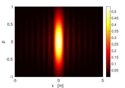
Figure 1: Magnitude of the WDF of a 1D Gauss-Schell correlation function. The radiation frequency is $f=1$ GHz corresponding to $\lambda=0.3$ m. The distribution widths are $\sigma_{x}=1.0$ m, and $\sigma_{s}=0.1$ m.

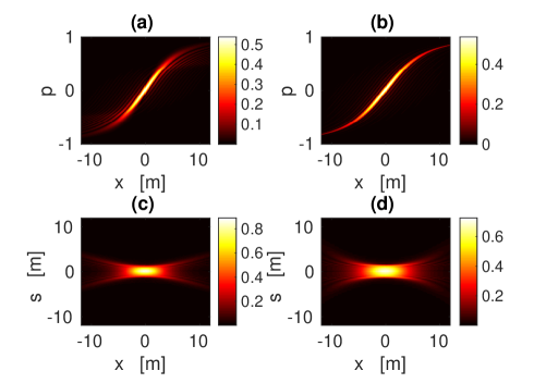
Figure 2: Propagated Wigner distribution function (a), (b) and correlation function (c), (d) of a partially-coherent (1D Gauss-Schell) near-homogeneous source: exact ((a) and (c)) vs approximate - Frobenius-Perron - ((b) and (d)) computation at $z=10\lambda$. The radiation frequency is $f=1$ GHz. The distribution widths are $\sigma_{x}=1$ m, and $\sigma_{s}=0.1$ m.

Fig. 2 shows the propagation of (19) as computed through the full integral operator (7) together with the propagation obtained by the Frobenius-Perron approximation (12). There is surprisingly good agreement between the exact and approximate behaviour even far from the paraxial regime. This is remarkable given that the ray tracing approximation is only valid to leading order. This constitutes a major computational advantage as the FP approximation reduces an integral equation to a simple coordinate transformation. The overall behaviour shown in Fig. 2(a) and Fig. 2(b) reflects the distribution shearing due to the geometrical ray propagation based on Eq. (13); see also Alonso (2011). The CFs can now be obtained by a back transformation according to Eq. (9) and are shown in Fig. 2(c) and Fig. 2(d).

IV.2 Non-paraxial Van Cittert-Zernike theorem

In the following, we will focus on near-field effects for small distances from the source as a function of the source correlation parameter $\sigma_{s}$. We are in particular interested in how the correlation length propagates in the near- field before reaching the linear VCZT regime.

In the near-field limit, the WDF shows exponentially decaying evanescent components according to (16), while the WDF remains essentially unchanged for the propagating part $|p|^{2}<1$. This leads to a model for the WDF with source distribution (20) of the form

$$\begin{split}W_{z}(x,p)\approx\sqrt{2\pi}\sigma_{s}I_{0}\exp\left[-\frac{x^{2}}{2\sigma^{2}_{x}}-\frac{k^{2}p^{2}\sigma^{2}_{s}}{2}\right]\\ \times\left\{\begin{array}[]{ll}1&\mbox{if $|p|^{2}<1$}\\ {\rm e}^{-2kz\sqrt{|p|^{2}-1}}&\mbox{if $|p|^{2}>1$}\,.\end{array}\right.\end{split}$$ (21)

Far enough from the source, such that evanescent components have completely decayed, while close enough that evolution in the propagating region of phase space can still be neglected, we model the WDF using

$$\begin{split}W_{z}(x,p)\approx\sqrt{2\pi}\sigma_{s}I_{0}\exp\left[-\frac{x^{2}}{2\sigma^{2}_{x}}-\frac{k^{2}p^{2}\sigma^{2}_{s}}{2}\right]\\ \times\left\{\begin{array}[]{ll}1&\mbox{if $|p|^{2}<1$}\\ 0&\mbox{if $|p|^{2}>1$}.\end{array}\right.\end{split}$$ (22)

Using the inverse Fourier transform, Eq.  (9), we now obtain the correlation function from the WDF given by Eq. (21) or Eq. (22) acccordingly. In Fig. 3 we show the resulting near-field evolution of the correlation function, placing the midpoint ${x}=({x}_{A}+{x}_{B})/2=0$ at the centre of the source.

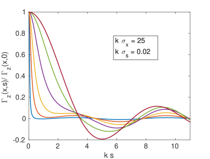
Figure 3: Evolution of the correlation function along the line $x=0$ for a selected (partially) correlated source, from $kz=0.42$ (blue solid line) to $kz=1.68$ (brown solid line). In the presence of evanescent waves the correlation width increases rapidly before the correlation function becomes a sinc function, whose width then increases linearly according to the VCZT.

One observes that in the near-field regime, the width $\Delta s$ of the correlation function is smaller than $\lambda$, but it increases rapidly towards $\lambda$ as $z$ approaches and exceeds $\lambda$. The second moment of the correlation function is not defined and cannot therefore be used to define a correlation length. Instead, we define the correlation lengths to be the spacing at which the correlation has fallen by a factor $1/\sqrt{{\rm e}}$:

$$\Gamma_{z}(x+\Delta s/2,x+\Delta s/2)/\Gamma_{z}(x,x)={\rm e}^{-1/2}.$$ (23)

Note that for a Gaussian correlation function such as assumed for the source in (17), this definition coincides with the standard variance: $\Delta s=\sigma_{s}$.

With the definition adopted above, we can now obtain the correlation lengths from exact wave propagation calculations. The results are shown in Fig. 4 as a function of the distance $z$ for different source correlation lengths $\sigma_{s}$. The universal regime is shown as the blue dashed line. The VCZT regime starts around $kz>1$.

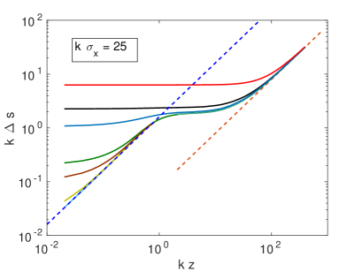
Figure 4: Evolution of the correlation length $\Delta s$ with z on a log-log scale at $x=0$ and for a partially correlated 1D source with $k\sigma_{s}=0.002$ (cyan solid line)$\ldots 6.3$ (red solid line). Evanescent waves drive the rapid spatial (blue dashed line) increase preceding the VCZT regime (red dashed line). A plateau is observed between $kz\approx 1$ and the Rayleigh range discovered in Cerbino (2007); Gatti (2008).

From Eqs. (21) and (22), one can estimate the growth rate both in the near and the far field. Including non-paraxial effects, there are three different regimes:

• in the deep near field, with $kz<1$ and $k\sigma_{s}<1$, the correlation length increases linearly with a slope that is independent of the frequency as well as of $\sigma_{s}$ and $\sigma_{x}$;

• a no-growth regime with $\Delta s=const$.

  • For $k\sigma_{s}<1$, one finds $k\Delta s\approx 1$ in the range $1<kz<k\sigma_{x}$;
    

  • For $k\sigma_{s}>1$, then $\Delta s=\sigma_{s}$ in the range $0<z<k\sigma_{x}$.

  The latter regime has already been described by Cerbino for paraxial sources Cerbino (2007);

• the VCZT regime for large $z$ with a linear growth of the correlation length according to

  $$\Delta s\propto\frac{\lambda}{\ell}z\,,$$ (24)

  with a slope depending on the ratio of wavelength to source dimension $\ell$.

We now motivate these three regimes in more detail, beginning with case (i), which corresponds to $k\sigma_{s}<1$, $kz<1$. The WDF $W_{z}({x},{p})$ described by (21) then decays slowly along the $p$ axis as $|p|$ increases beyond the propagating region $|p|^{2}<1$. In the extreme nearfield the correlation function is proportional to the inverse Fourier transform of the function

$$W_{z}(x,p)\sim{\rm e}^{-2kz|p|}$$

of $p$, that is,

$$\Gamma_{z}(s)\sim\frac{2kz/\pi}{(2kz)^{2}+(ks)^{2}}.$$

The correlation length defined by Eq.  (23) then takes the form

$$\Delta s\approx 2\sqrt{\sqrt{{\rm e}}-1}\;z\approx 1.6109\,z.$$ (25)

That is, we find in regime (i) that evanescent decay of the sub-wavelength correlations in the source dominates in such a way that there is a universal growth rate in the correlation length. The numerical value of the slope in (25) is particular to the form taken in Eq.  (23) for the correlation length, but the qualitative conclusion applies more generally. The presence of evanescent waves thus leads to a rapid increase of the correlation length in the near field in this regime. This is important for sources that show fluctuations on scales smaller than the wavelength, such as in the case of a fully uncorrelated source $\sigma_{s}=0$, which may serve as a model for thermal sources Carminati and Greffet (1999).

The plateau behaviour corresponding to regime (ii) arises when $z$ is sufficiently large that (22) describes the WDF, while $k\sigma_{s}\ll 1$. The correlation function is then proportional to the inverse Fourier transform

$$\Gamma_{z}(s)\sim\frac{1}{\pi}{\rm sinc}(ks)$$

of the function

$$W_{z}(x,p)\sim\begin{cases}1,&\qquad|p|^{2}<1,\\ 0,&\qquad|p|^{2}>1\end{cases}$$ (26)

of $p$. In this case the correlation length defined by Eq.  (23) takes the form

$$k\Delta s\approx 1.6443$$ (27)

independent of $\sigma_{s}$. It should be noted that if the condition $k\sigma_{s}<1$ is breached, then the Gaussian decay in $p$ present in (22) becomes the dominant feature and instead a limiting plateau level

$$\Delta s=\sigma_{s}$$

occurs, see Fig. 4. Note that in this case the plateau extends all the way to $z=0$ and the linear regime of case (i) is not seen.

Finally, regime (iii) applies once evolution of the phase space takes effect in the propagating region $|p|^{2}<1$. Assuming the quasihomogeneous case $\sigma_{x}\gg l$ and considering first only the near-field region $k\sigma_{s}\ll kz\ll 1$, then for a given midpoint $x$ the finite size of the source reduces the support in $p$ of the Wigner function and (26) is replaced by

$$W_{z}(x,p)\sim\begin{cases}1,&\qquad\frac{x-l/2}{\sqrt{z^{2}+(x-l/2)^{2}}}<p<\frac{x+l/2}{\sqrt{z^{2}+(x+l/2)^{2}}},\\ 0,&\qquad\mbox{otherwise}.\end{cases}$$

For simplicity consider the case $x=0$. Then the correlation function obtained from the inverse Fourier transform of this function is

$$\Gamma_{z}(s)\sim\frac{1}{\pi}{\rm sinc}\left(\frac{ks}{\sqrt{1+(2z/l)^{2}}}\right)$$

and the correlation length defined by (23) takes the form

$$\Delta s\approx 0.2617\lambda\sqrt{1+(2z/l)^{2}},$$ (28)

generalising (27). In the farfield $z\gg l$, we find

$$\Delta s\approx 0.2617\times\frac{2z\lambda}{l}$$

(where the numerical prefactor is particular to the convention (23)). Alternatively, if $\sigma_{x}\gg l$, then the screen length becomes unimportant and $\sigma_{x}$ provides the length scale appropriate to the source intensity. An analogous calculation then allows us instead to recover the basic form

$$\Delta s\approx\frac{1}{2\pi}\times\frac{z\lambda}{\sigma_{x}}$$

of the VCZT for $z\gg\sigma_{x}$.

IV.3 Application to a complex source

The field at the source at $z=0$ is often produced by a complex process such as tracks on a printed circuit board or integrated circuits in electronic devices; the radiation produced in the source region then propagates into free space. We model such a complex source here by a set of $N$ metallic wires driven by random time-domain voltages, as illustrated in Fig. 5; a realization of the voltage $s_{p}\left(t\right)$ driving a pin of the bundle is reported in Fig. 6 along with its spectrum $S_{p}\left(f\right)$.

\psfrag{pec}{{PEC}}\psfrag{x}{$x$}\psfrag{y}{$y$}\psfrag{z}{$z$}\psfrag{sp}{$s_{p}(t)$}\psfrag{d}{$d$}\psfrag{l}{$l$}\psfrag{hl}{$h_{l}$}\psfrag{hu}{$h_{u}$}\includegraphics[width=108.405pt]{scheme2.eps}

Figure 5: Set of parallel metallic wires running above an oblique perfect electric conductor (PEC) ground plane. This complex source emits radiation in the half-space $z>0$. The full-wave TLM simulation has been carried out for the configuration $h_{l}=0.3025$ m, $h_{u}=0.358$ m, $l=1$ m, $d=0.06$ m.

T

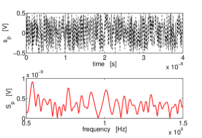
Figure 6: Time- and frequency-domain behavior of the signal driving a pin of the bundle.

This represents a typical problem in EMC where one tries to obtain statistical information about an erratic signal.

The presence of a perfect electric conductor along an oblique plane makes the source radiate only into the half-space $z>0$: this mimics a configuration that is widely used in the design of printed circuit boards. We use $N=12$ wires very close to each other and to the metallic plane in terms of wavelength. Therefore, it is reasonable to think of this circuit as a collection of random sources of partially coherent radiation.

The exact fields emitted from such a complex structure are computed through an in-house Transmission Line Matrix (TLM) code Christopoulos (1995). This is a time domain method for modelling 3D electromagnetic field interactions with complex structures that may include a variety of materials. The technique is based on the equivalence between electric and magnetic fields and the voltages and currents on a network of transmission lines. After discretizing space, the fields in individual cells are modelled by transmission lines incident from each cell-face and intersecting at the cell centre forming a junction. Each of these orthogonal transmission lines allows for the propagation of electromagnetic waves. The waves are characterised by voltage and current and their associated electric and magnetic fields. In order to obtain the desired correlation functions, we sample the numerically obtained fields in a plane above the tracks at different times in order to create a suitable ensemble of uncorrelated circuit realisations. This is used as a basis for calculating field-field correlation functions and their Wigner functions both in the near- and far-field.

Figs. 7 (a) and (b) show the comparison between the WDF as computed through the full-wave (TLM) simulations, and the WDF obtained by the FP approximation (12) in the far-field at $z=2.3\lambda$. In the TLM calculation, the full time-dependent field is propagated out from the source, while in the FP approximation, the WDF obtained from the signal at the source (as shown in Fig. 6, see also Fig. 8 (a)) is propagated according to (12). There is good agreement between the behavior predicted from full-wave simulations and the FP approximation, even though the source exhibits strong inhomogeneities. Interestingly, Fig. 7 shows the same Wigner distribution shearing as in Fig. 2 following the geometrical interpretation (13) of the correlation propagation. It is worth stressing that such a Wigner function challenges the FP approximation (12), whose underlying assumption is quasi-homogeneity. Note that we can always also switch to the exact transport rule (7), which is computationally more expensive than the FP approximation, but still orders of magnitudes faster than a full TLM calculation. Propagated CFs as shown in Fig. 7 (lower plots (c) and (d)) are finally obtained by applying the inverse Fourier transform (9).

Note that we also find a pronounced broad side radiation around $p\approx\pm 1$ (corresponding to $\alpha\approx\pm\pi/2$), and a strong asymmetry of the Wigner distribution due to the oblique metallic reflector. Those features can be captured by inspection of the WDF representation in phase-space, while they are less apparent in the propagated correlation function shown in Fig. 7 (c) and (d).

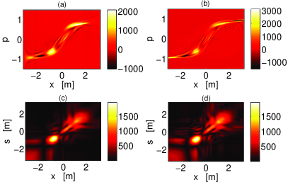
Figure 7: Far-field WDF (upper plots) and correlation functions (lower plots) at $z=2.3$ $\lambda$: comparison between TLM computation (left column) and Frobenius-Perron analytical approximation (12) (right column). The propagated correlation has been calculated through (9).

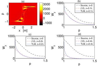
Figure 8: (a) Source distribution; near-field WDF: comparison between TLM computation and evanescent-wave approximation (16) for (b) $z=0.1\lambda$; (c) $z=0.2\lambda$ and (d) $z=0.4\lambda$ along $x=0$.

The source distribution $W_{0}(x,p)$ as obtained from the radiated signal, see Fig.  6, is shown in Fig. 8 (a). Note that the region with $|p|^{2}>1$ corresponds to evanescent contributions. In Fig. 8 (b)-(d), a comparison between WDFs as computed through the full-wave (TLM) simulations and those obtained using the WDF propagator incorporating evanescent contributions, Eq. (16), are shown along the line $x=0$. We find that propagation beyond $z=0.1\,\lambda$ results predominantly in an exponential reduction of the WDF in the region $|p|^{2}>1$. In the far-field, the radiation energy is restricted to the phase-space region $\left|{p}\right|<1$, as can be seen in the WDF in Fig. 7 (a) and (b).

A comparison of (TLM) simulated and (Frobenius-Perron) approximate far-field propagated energy

$$E_{z}=\frac{1}{2}\,\epsilon_{0}\,\left|\phi\left(x\right)\right|^{2}=\frac{1}{2}\,\epsilon_{0}\,\int\,W_{z}\left(x,p\right)\,dp,$$ (29)

is shown in Fig. 9. We see that the two numerical methods show qualitatively the same features, however, there are quantitative differences. We think that these deviations are due to a difference in the numerical treatment of the boundary conditions at $x=\pm 3$ m. While the FP approach has no difficulties in treating these boundaries as completely open, the TLM method needs to model this with absorbing boundary conditions. These conditions tend to be still slightly reflective, as is evident from the source distribution in Fig. 8 (a) around $x=\pm 3$, $p=\pm 1$. This comparison highlights another advantage of the Wigner function propagation method.

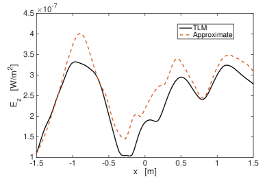
Figure 9: TLM versus approximate energy density of the field radiated far from the source.

The evaluation of the WDF of actual circuits can be done for the full electromagnetic field by using the approach described here component by component.

V Reflection of partially correlated sources

Having developed a framework for the propagation of CFs in free space, we are now interested in tackling the case of reflection from planar boundaries. In particular we would like to test the FP approximation in the presence of interference. It is then interesting to solve the canonical situation depicted in Fig. 10, where a planar reflector is located at distance $z=L$ from the source at $z=0$.

The reflecting boundary is here for simplicity assumed to be parallel to the source plane, indefinitely extended in the $\hat{xy}$-plane, and made of an ideal perfect electric conductor (PEC). Therefore, for electric (TE) or magnetic (TM) fields perpendicular to $\hat{z}$, the Fresnel reflection coefficient reads $r\left(\alpha\right)=-1$, for all incoming angles $\alpha$ Tsang and Kong (2004). We again consider for simplicity only a scalar field, or a single component of the vector field, emitted from the source.

V.1 Theory

\psfrag{x}{\small$\hat{x}$}\psfrag{y}{\small$\hat{y}$}\psfrag{z}{\small$\hat{z}$}\psfrag{s}{\small Planar source}\psfrag{d}{\small Scan plane}\psfrag{l}{\small Reflector}\psfrag{del}{\small$\Delta$}\psfrag{pec}{\small PEC}\psfrag{z0}{\small$z=0$}\psfrag{zd}{\small$z=D$}\psfrag{p1}{\small$\hat{\phi}\left(\ushortw{p}_{1},z\right)$}\psfrag{zl}{\small$z=L$}\psfrag{a1}{\small$\alpha_{1}$}\psfrag{d}{\small Detector}\includegraphics[width=176.407pt]{FS_source_ref.eps}

Figure 10: Arbitrary planar electromagnetic source emitting in the half-space $z>0$, in presence of a planar metallic boundary.

Consider a plane located at an arbitrary longitudinal coordinate $z=D$ between source and detector. The field distribution in the plane consists then of two contributions: the direct wave coming from the source, and the reflected wave bouncing off the reflector back to the source, that is,

$$\hat{\phi}\left(p,z\right)={\rm e}^{rmikDT(p)}\phi\left(p,0\right)-{\rm e}^{{\rm i}kDT(p)+i2k\Delta T(p)}\phi\left(p,0\right),$$ (30)

where $\phi\left(p,0\right)$ is the field at the source plane $z=0$, $T(p)$ is defined as in (3), and $\Delta=L-D$. The momentum space CF is formed as the product of the two fields in (30) and an ensemble average is taken as in Eq. (1). By plugging the closed-form expression (30) into the definition of the WDF (6), we find the phase space representation

$$\small\mathcal{W}_{D}\left(p,x\right)=W_{D}\left(p,x\right)+W_{2L-D}\left(p,x\right)-\left[W_{\Delta}\left(p,x\right)+\textrm{cc}\right],$$ (31)

where the first two terms are direct and reflected contributions respectively, coming to the detector straight from the source or through the reflector, and the last two terms express the interference between direct and reflected waves with cc standing for the complex conjugate.

Following the procedure described in the previous subsection, it can be shown that direct and reflected terms in (31) can be calculated through the free-space propagation scheme in (7) and (8), with $z=D$ and $z=2L-D$ respectively, while the interference terms lead to

$$W_{\Delta}\left(p,x\right)=\iint\,\mathcal{G}_{\Delta}\left(x,x^{\prime};p,p^{\prime}\right)\,W_{0}\left(x^{\prime},p^{\prime}\right)\,{\rm d}x^{\prime}{\rm d}p^{\prime}\,\,,$$ (32)

with a modified Green integral operator

$$\mathcal{G}_{\Delta}\left(x,x^{\prime};p,p^{\prime}\right)=\delta\left(p-p^{\prime}\right)\frac{1}{(2\pi)^{2}}$$ (33)

$$\times\int\,{\rm e}^{{\rm i}k\left(x-x^{\prime}\right)q+{\rm i}kD\left(T(p+\frac{q}{2})-T^{*}(p-\frac{q}{2})\right)-{\rm i}2k\Delta T^{*}(p-\frac{q}{2})}\,{\rm d}q\,\,.$$

For the class of statistically quasi-homogeneous sources, we may again expand the exponent in (33) in a Taylor series in $q$, and retain only terms up to first order. This results in a Frobenius-Perron approximation of the interference terms, leading to a phase-factor of the optical length $\Delta$ besides the Dirac’s delta in (11). Adopting the same linear approximation for each term in (31) gives the updated WDF

$$\mathcal{W}_{D}\left(x,p\right)\approx W_{0}\left(x-\frac{Dp}{T(p)},p\right)$$ (34)

$$+\left.W_{0}\left(x-\frac{\left(2L-D\right)p}{T(p)},p\right)\right.$$

$$-2\cos\left(2k\Delta T\left(p\right)\right)\,W_{0}\left(x-\frac{Lp}{T(p)},p\right).$$

Similar expressions have been found in quantum mechanics Littlejohn (1986) and optics Torre (2005) for two overlapping wave-functions.

Again, the propagated CF can be obtained by the inverse Fourier transform (9) of (31) or (34), the latter being closely related to the free-space VCZT.

V.2 Numerical results

We chose again an initial correlation density distributed according to the Gauss-Schell model, Eq. (17), with corresponding source WDF shown in Fig. 1. We work as usual at a frequency of operation of $1$ GHz corresponding to $\lambda=0.3$ m and choose $\sigma_{x}=1.0$ m, $\sigma_{s}=0.1$ m.

We further suppose a metallic mirror at $L=1.8$ m ($6\lambda$). The propagation of the intensity from the source to the mirror can be found by evolving the source WDF with the exact rule composed of Eqs. (7), (8) and those for the interference terms, Eqs. (31) – (33), and then inverse Fourier transforming the propagated WDF according to Eq.  (9). The coherent energy $I_{z}(x)$ reaching the scan plane at $z=D$ is given by Eq. (10), that is, by considering the correlation function at $s=0$.

Figure 11 shows the behavior of the intensity $I_{z}(x=0)$ near the mirror, from $D=1.0$ m to $D=1.8$ m. The solid black line is computed through the full Green’s integral operators (31) and (33), while the dashed red line is obtained by the Frobenius-Perron approximation (34).

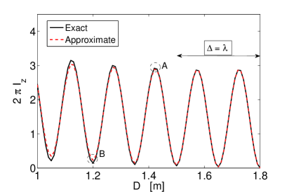
Figure 11: Interference pattern formed by the intensity $I_{z}$ ($x=0$) along the longitudinal direction as the scan plane approaches the reflector. Exact (black solid line) versus approximate (red dashed line) computations are compared.

The oscillatory behaviour in (34) is due to the interference terms in the WDF.

In Figs. 12 and 13, we show the magnitude of the WDF and the associated CFs at a distance $\Delta=1.25\lambda$ (position A in Fig. 11) and at a distance $\Delta=2\lambda$ (position B in Fig. 11) from the mirror, respectively. While good agreement between the exact and the approximate propagation using the FP approximation is achieved at position A, a maximum in the correlation function, the same is not true at position B. Here the intensity is suppressed due to destructive interference and the magnitude of the CF is itself only of order $O(1/k)$. To obtain the good agreement shown in Fig. 13, we need to take into account higher order corrections in the WDF propagator such as using the Airy function integral kernel, Eq. (15). The improvement when going from the leading order FP to the Airy function approximation is shown in Fig. 13 (b) to (c), which need to be compared with the exact WF Fig. 13 (a); the corresponding propagated CF is displayed in Fig. 13 (d). Only after going beyond the FP approximation in this way are we able to reconstruct the fine structure of the WDF. This finding is not surprising, but remarkable nevertheless; computing WDFs in a multi-scattering environment will encounter exactly these problems and we have shown that the Airy-function approximation - still faster than a full WDF propagation - can handle interference corrections successfully. We note that these corrections have been reported also in the “diffusive” Green function presented in Marcuvitz (1991).

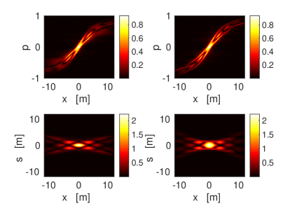
Figure 12: Magnitude of the WDF of a 1D Gauss-Schell source: exact (left plots) versus approximate (right plots) computation at $\Delta=1.25\lambda$ (position A in Fig. 11). Related correlation functions are reported in the lower plots.

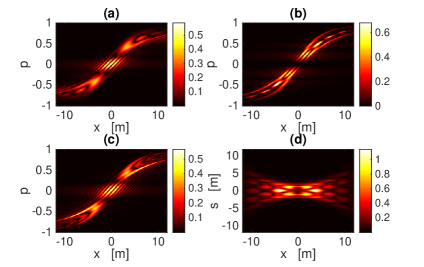
Figure 13: Magnitude of the WDF of a 1D Gauss-Schell source: exact (a) versus approximate using only FP approximation (b) and using the Airy approximation (c) at $\Delta=2\lambda$ (position B in Fig. 11). The correlation function corresponding to (c) is reported in (d).

VI Conclusion

An exact propagator has been derived for field-field correlation functions of complex sources. It has been applied to a problem mimicking EM radiation from a complex source; extending this to other wave problems such as in vibro-acoustics or quantum mechanics is straightforward. The phase-space representation based on the Wigner function provides a useful means of physically interpreting the propagated data. It also serves as a very efficient computational technique both for an exact propagation of CFs and in terms of a ray approximation leading to the Frobenius-Perron operator. This provides a good description of the propagated data even when applied to source data that are relatively far from homogeneity. Where necessary, more heterogeneous sources can be accounted for by higher-order approximations leading to an Airy propagator. This propagator proved important in the case of a planar random source emitting in presence of a planar reflector, for which we are able to reconstruct the fine structure of the phase space in presence of interference. Evanescent decay into the near field can also be accounted for using simple propagation rules. These rules has been used to investigate the effect of evanescent waves in near-field correlation functions. For source correlations exhibiting smaller-than-wavelength scales, we predicted a rapid initial increase of the correlation length (with distance from the source), before it saturates with the onset of the Van Cittert-Zernike behaviour at a distance of a wavelength. The approximations used have been validated through full-wave simulations using model sources and numerical sources exhibiting strong statistical inhomogeneities.

VII Acknowledgments

Financial supported through by the EPSRC (Grant-Ref.: EP/K019694/1) is gratefully acknowledged.

References

- Tanner and Mace (2014) G. Tanner and B. Mace, Wave Motion 51, 547 (2014), ISSN 0165-2125, Innovations in Wave Modelling.
- Montrose (2004) M. Montrose, EMC and the Printed Circuit Board: Design, Theory, and Layout Made Simple, IEEE Press Series on Electronics Technology (Wiley, 2004), ISBN 9780471660903.
- Hillery et al. (1984) M. Hillery, R. O’Connell, M. Scully, and E. Wigner, Physics Reports 106, 121 (1984), ISSN 0370-1573.
- Dragoman (1997) D. Dragoman, Progress in Optics XXXVII (Elsevier, 1997).
- Torre (2005) A. Torre, Linear Ray and Wave Optics in Phase Space: Bridging Ray and Wave Optics via the Wigner Phase-Space Picture (Elsevier Science, 2005), ISBN 9780080535531.
- Alonso (2011) M. A. Alonso, Adv. Opt. Photon. 3, 272 (2011).
- Alonso (2004) M. A. Alonso, J. Opt. Soc. Am. A 21, 2233 (2004).
- Chappell et al. (2013) D. J. Chappell, G. Tanner, D. Löchel, and N. Søndergaard, Proceedings of the Royal Society A: Mathematical, Physical and Engineering Science 469 (2013).
- Dittrich and Pachón (2009) T. Dittrich and L. A. Pachón, Phys. Rev. Lett. 102, 150401 (2009).
- Berry (1977a) M. V. Berry, J. Phys. A: Math. Gen. 10, 2083 (1977a).
- Hemmady et al. (2012) S. Hemmady, T. M. Antonsen, E. Ott, and S. M. Anlage, IEEE Trans. Electromag. Compat. 99, 1 (2012).
- Creagh and Dimon (1997) S. C. Creagh and P. Dimon, Phys. Rev. E 55, 5551 (1997).
- Hortikar and Srednicki (1998) S. Hortikar and M. Srednicki, Phys. Rev. Lett. 80, 1646 (1998).
- Weaver and Lobkis (2001) R. L. Weaver and O. I. Lobkis, Phys. Rev. Lett. 87, 134301 (2001).
- Urbina and Richter (2006) J. D. Urbina and K. Richter, Phys. Rev. Lett. 97, 214101 (2006).
- Cerbino (2007) R. Cerbino, Phys. Rev. A 75, 053815 (2007).
- Gatti (2008) A. Gatti and D. Magatti and F. Ferri, Phys. Rev. A 78, 063806 (2008).
- Jackson (1998) J. Jackson, Classical Electrodynamics (Wiley, 1998), ISBN 9780471309321.
- Bucci and Franceschetti (1987) O. Bucci and G. Franceschetti, Antennas and Propagation, IEEE Transactions on 35, 1445 (1987), ISSN 0018-926X.
- Arnaut et al. (2013) L. Arnaut, C. Obiekezie, and D. Thomas, Electromagnetic Compatibility, IEEE Transactions on PP, 1 (2013).
- Russer and Russer (2012) J. Russer and P. Russer, in Electromagnetic Compatibility (APEMC), 2012 Asia-Pacific Symposium on (2012), pp. 709–712.
- Feng et al. (1988) S. Feng, C. Kane, P. A. Lee, and A. D. Stone, Phys. Rev. Lett. 61, 834 (1988).
- Crisanti et al. (1993) A. Crisanti, M. H. Jensen, A. Vulpiani, and G. Paladin, Phys. Rev. Lett. 70, 166 (1993).
- Luis (2007) A. Luis, Phys. Rev. A 76, 043827 (2007).
- Harrington (1961) R. F. Harrington, Time-Harmonic Electromagnetic Fields (McGraw-Hill Book Company, New York, 1961), 1st ed.
- Creagh et al. (2013) S. C. Creagh, H. B. Hamdin, and G. Tanner, Journal of Physics A: Mathematical and Theoretical 46, 435203 (2013).
- Berry (1977b) M. V. Berry, Philosophical Transactions of the Royal Society of London. Series A, Mathematical and Physical Sciences 287, 237 (1977b).
- de M Rios and de Almeida (2002) P. P. de M Rios and A. M. O. de Almeida, Journal of Physics A: Mathematical and General 35, 2609 (2002).
- Dittrich et al. (2006) T. Dittrich, C. Viviescas, and L. Sandoval, Phys. Rev. Lett. 96, 070403 (2006).
- Ott (2002) E. Ott, Chaos in dynamical systems (Cambridge University Press, 2002).
- Littlejohn and Winston (1993) R. G. Littlejohn and R. Winston, J. Opt. Soc. Am. A 10, 2024 (1993).
- Winston et al. (2002) R. Winston, Y. Sun, and R. G. Littlejohn, Optics Communications 207, 41 (2002), ISSN 0030-4018.
- Marcuvitz (1991) N. Marcuvitz, Proceedings of the IEEE 79, 1350 (1991).
- Wolf (2007) E. Wolf, Introduction to the Theory of Coherence and Polarization of Light (Cambridge University Press, 2007), ISBN 9780521822114.
- Carminati and Greffet (1999) R. Carminati and J.-J. Greffet, Phys. Rev. Lett. 82, 1660 (1999).
- Gori et al. (2001) F. Gori, M. Santarsiero, G. Piquero, R. Borghi, A. Mondello, and R. Simon, Journal of Optics A: Pure and Applied Optics 3, 1 (2001).
- Bastiaans (1979) M. Bastiaans, Optics Communications 30, 321 (1979), ISSN 0030-4018.
- Tsang and Kong (2004) L. Tsang and J. Kong, Scattering of Electromagnetic Waves, Advanced Topics, Scattering of Electromagnetic Waves (Wiley, 2004), ISBN 9780471463795.
- Littlejohn (1986) R. G. Littlejohn, Physics Reports 138, 193 (1986), ISSN 0370-1573.
- Christopoulos (1995) C. Christopoulos, The Transmission-line Modeling Method: TLM, IEEE/OUP series on electromagnetic wave theory (IEEE, 1995), ISBN 9780198565338.
- Winston et al. (2006) R. Winston, A. D. Kim, and K. Mitchell, Journal of Modern Optics 53, 2419 (2006).