Bias correction in multivariate extremes

Abstract

The estimation of the extremal dependence structure is spoiled by the impact of the bias, which increases with the number of observations used for the estimation. Already known in the univariate setting, the bias correction procedure is studied in this paper under the multivariate framework. New families of estimators of the stable tail dependence function are obtained. They are asymptotically unbiased versions of the empirical estimator introduced by Huang [Statistics of bivariate extremes (1992) Erasmus Univ.]. Since the new estimators have a regular behavior with respect to the number of observations, it is possible to deduce aggregated versions so that the choice of the threshold is substantially simplified. An extensive simulation study is provided as well as an application on real data.

FLA

,
and T1Supported in part by the Agence Nationale de la Recherche through the AST&RISK project (ANR-08-BLAN-0314-01), and by FCT/PTDC/MAT/112770/2009 (Portugal).

1 Introduction

Estimating extreme risks in a multivariate framework is highly connected with the estimation of the extremal dependence structure. This structure can be described via the stable tail dependence function (s.t.d.f.) $L$, first introduced by Huang (1992). For any arbitrary dimension $d$, consider a multivariate vector $(X^{(1)},\ldots,X^{(d)})$ with continuous marginal cumulative distribution functions (c.d.f.) $F_{1},\ldots,F_{d}$. The s.t.d.f. is defined for each positive reals $x_{1},\ldots,x_{d}$ as

$$\lim_{t\to\infty}t\mathbb{P}\bigl{\{}1-F_{1}\bigl{(}X^{(1)}\bigr{)}\leq t^{-1}x_{1}\mbox{ or }\ldots\mbox{ or }1-F_{d}\bigl{(}X^{(d)}\bigr{)}\leq t^{-1}x_{d}\bigr{\}}$$

$$\qquad=L(x_{1},\ldots,x_{d}).$$

Assuming that such a limit exists and is nondegenerate is equivalent to the classical assumption of existence of a multivariate domain of attraction for the componentwise maxima; see, for example, de Haan and Ferreira (2006), Chapter 7. The previous limit can be rewritten as

$$\lim_{t\to\infty}t\bigl{[}1-F\bigl{\{}F_{1}^{-1}\bigl{(}1-t^{-1}x_{1}\bigr{)},\ldots,F_{d}^{-1}\bigl{(}1-t^{-1}x_{d}\bigr{)}\bigr{\}}\bigr{]}=L(x_{1},\ldots,x_{d}),$$ (1)

where $F$ denotes the multivariate c.d.f. of the vector $(X^{(1)},\ldots,X^{(d)})$, and for $j=1,\dots,d$, $F_{j}^{-1}(t)=\inf\{z\in{\mathbb{R}}\dvtx F_{j}(z)\geq t\}$. Consider a sample of size $n$ drawn from $F$ and an intermediate sequence, that is to say a sequence $k=k(n)$ tending to infinity as $n\to\infty$, with $k/n\to 0$. Denote by ${\mathbf{x}}=(x_{1},\ldots,x_{d})$ a vector of the positive quadrant $\mathbb{R}^{d}_{+}=\{(x_{1},\ldots,x_{d})\dvtx x_{j}\geq 0,j=1,\dots,d\}$ and by $X^{(j)}_{k,n}$ the $k$th order statistics among $n$ realizations of the margins $X^{(j)}$. The empirical estimator of $L({\mathbf{x}})$ is obtained from (1), replacing $F$ by its empirical version, $t$ by $n/k$, and $F_{j}^{-1}(1-t^{-1}x_{j})$ for $j=1,\ldots,d$ by its empirical counterpart $X^{(j)}_{n-[nt^{-1}x_{j}],n}$, so that

$$\hat{L}_{k}({\mathbf{x}})=\frac{1}{k}\sum_{i=1}^{n}\mathbh{1}_{\{X^{(1)}_{i}\geq X^{(1)}_{n-[kx_{1}]+1,n}~{}\mathrm{or}~{}\ldots~{}\mathrm{or}~{}X^{(d)}_{i}\geq X^{(d)}_{n-[kx_{d}]+1,n}\}}.$$ (2)

See Huang (1992) for pioneering works on this estimator. Under suitable conditions, it can be shown (see Section 2) that the estimator $\hat{L}_{k}({\mathbf{x}})$ has the following asymptotic expansion:

$$\hat{L}_{k}({\mathbf{x}})-L({\mathbf{x}})\approx\frac{Z_{L}({\mathbf{x}})}{\sqrt{k}}+\alpha(n/k)M({\mathbf{x}}),$$ (3)

where $Z_{L}$ is a continuous centered Gaussian process, $\alpha$ is a function that tends to 0 at infinity and $M$ is a continuous function. In particular$\sqrt{k}\{\hat{L}_{k}({\mathbf{x}})-L({\mathbf{x}})\}$ can be approximated in distribution by $Z_{L}({\mathbf{x}})$, provided that $\sqrt{k}\alpha(n/k)$ tends to 0 as $n$ tends to infinity. This condition imposes a slow rate of convergence of the estimator $\hat{L}_{k}({\mathbf{x}})$, so one would be interested in relaxing this hypothesis. As a counterpart, as soon as $\sqrt{k}\alpha(n/k)$ tends to a nonnull constant $\lambda$, an asymptotic bias appears and is explicitely given by $\lambda M({\mathbf{x}})$. The aim of this paper is to provide a procedure that reduces the asymptotic bias. The latter will be estimated and then subtracted from the empirical estimator. This kind of approach has been considered in the univariate setting for the bias correction of the extreme value index with unknown sign by Cai, de Haan and Zhou (2013). Refer also to Peng (1998, 2010) Fraga Alves, de Haan and Lin (2003), Gomes, de Haan and Rodrigues (2008) and Caeiro, Gomes and Rodrigues (2009) for previous contributions on this problem. Note finally that the case of dependent sequences has been recently studied by de Haan, Mercadier and Zhou (2014).

The nonparametric estimation of the extremal dependence structure has been widely studied in the bivariate case; see, for instance, Huang (1992), Einmahl, de Haan and Sinha (1997), Capéraà and Fougères (2000), Abdous and Ghoudi (2005), Guillotte, Perron and Segers (2011) and Bücher, Dette and Volgushev (2011). Bias correction problems in the bivariate context received less attention than in the univariate setting. To the best of our knowledge, it seems to be reduced to Beirlant, Dierckx and Guillou (2011) and Goegebeur and Guillou (2013), who consider the estimation of bivariate joint tails, which differs slightly from our task.

As for the multivariate framework, de Haan and Resnick (1993) introduces the empirical estimator. General approaches under parametric assumptions on the function $L$ have been developed, for example, by Coles and Tawn (1991), Joe, Smith and Weissman (1992), Einmahl, Krajina and Segers (2008) and Einmahl, Krajina and Segers (2012). Apparently, no procedure correcting the bias can be found in the literature for dimension greater than two. The objective of this article is to fill this gap. Note that our method does not only consist of applying the univariate bias procedure at several points. Indeed, the bias is no longer a parametric function, so that the new feature is mainly the fact that we are able to estimate and then subtract a function with an unknown form. Two families of asymptotically unbiased estimators of the s.t.d.f. are proposed, and their theoretical behaviors are studied. A practical advantage of these new estimators is that they can be aggregated, thus reducing the variability.

The paper is organized as follows: Section 2 contains hypotheses and first results. The bias reduction procedure is described in Section 3, and the main theoretical results are presented therein. Several theoretical models are exhibited in Section 4 that satisfy the required assumptions. Section 5 illustrates the performance of the new estimators on both simulated and real data. The estimation of side components is postponed up to Section 6. The proofs are relegated to Section 8.

2 Notation, assumptions and first results

Let ${\mathbf{X}}_{1}=(X^{(1)}_{1},\ldots,X^{(d)}_{1}),\break\ldots,{\mathbf{X}}_{n}=(X^{(1)}_{n},\ldots,X^{(d)}_{n})$ be independent and identically distributed multivariate random vectors with c.d.f. $F$ and continuous marginal c.d.f.’s $F_{j}$ for $j=1,\ldots,d$. Suppose $F$ is in the domain of attraction of an extreme value distribution with c.d.f. $G$. We recall that it supposes the existence for $j=1,\ldots,d$ of sequences $a_{n}^{(j)}>0$, $b_{n}^{(j)}$ of real numbers and a c.d.f. $G$ with nondegenerate marginals such that

$$\lim_{n\to\infty}\mathbb{P}\bigl{(}\max\bigl{\{}X^{(1)}_{1},\ldots,X^{(1)}_{n}\bigr{\}}\leq a^{(1)}_{n}x_{1}+b^{(1)}_{n},\ldots,$$

$$\hskip 54.0pt\max\bigl{\{}X^{(d)}_{1},\ldots,X^{(d)}_{n}\bigr{\}}\leq a^{(d)}_{n}x_{d}+b^{(d)}_{n}\bigr{)}=G({\mathbf{x}})$$

for all points ${\mathbf{x}}$ where $G$ is continuous. Denote by $G_{j}$ the $j$th marginal c.d.f. of $G$. It is possible to show that the domain of attraction condition can be expressed as condition (1) along with the convergence of the marginal distributions to the $G_{j}$’s, and that

$$L({\mathbf{x}})=-\log G\bigl{(}\{-\log G_{1}\}^{-1}(x_{1}),\ldots,\{-\log G_{d}\}^{-1}(x_{d})\bigr{)}.$$ (4)

Let $\mu$ be the measure defined by

$$\mu\bigl{\{}A({\mathbf{x}})\bigr{\}}:=L({\mathbf{x}}),$$ (5)

where $A({\mathbf{x}}):=\{{\mathbf{u}}\in\mathbb{R}_{+}^{d}$: there exists $j$ such that $u_{j}>x_{j}\}$ for any vector ${\mathbf{x}}\in\mathbb{R}_{+}^{d}$.

Several conditions are now described. The first two have been introduced by de Haan and Resnick (1993):

• [–]

• The first-order condition consists of assuming that the limit given in (1) exists, and that the convergence is uniform on any $[0,T]^{d}$, for $T>0$.

• The second-order condition consists of assuming the existence of a positive function $\alpha$, such that $\alpha(t)\to 0$ as $t\to\infty$, and a nonnull function $M$ such that for all ${\mathbf{x}}$ with positive coordinates,

  $$\lim_{t\to\infty}\frac{1}{\alpha(t)}\bigl{\{}t\bigl{[}1-F\bigl{\{}F_{1}^{-1}\bigl{(}1-t^{-1}x_{1}\bigr{)},\ldots,F_{d}^{-1}\bigl{(}1-t^{-1}x_{d}\bigr{)}\bigr{\}}\bigr{]}-L({\mathbf{x}})\bigr{\}}$$

  (6)

  $$\qquad=M({\mathbf{x}}),$$

  uniformly on any $[0,T]^{d}$, for $T>0$.

• The third-order condition consists of assuming the existence of a positive function $\beta$, such that $\beta(t)\to 0$ as $t\to\infty$, and a nonnull function $N$ such that for all ${\mathbf{x}}$ with positive coordinates,

  $$\lim_{t\to\infty}\frac{1}{\beta(t)}\biggl{\{}\frac{t[1-F\{F_{1}^{-1}(1-t^{-1}x_{1}),\ldots,F_{d}^{-1}(1-t^{-1}x_{d})\}]-L({\mathbf{x}})}{\alpha(t)}-M({\mathbf{x}})\biggr{\}}$$

  (7)

  $$\qquad=N({\mathbf{x}}),$$

  uniformly on any $[0,T]^{d}$, for $T>0$. This implicitly requires that $N$ is not a multiple of the function $M$; see Remark 2.

Remark 1.

The function $L$ defined by (1) and that appears in (– ‣ 2) and (– ‣ 2) is homogeneous of order 1. We refer, for instance, to de Haan and Ferreira (2006), pages 213 and 236. Most of the estimators constructed in this paper use the homogeneity property. Note that pointwise convergence in (1) entails uniform convergence on the square $[0,T]^{d}$. See, for instance, de Haan and Ferreira (2006), page 237.

Remark 2.

If $N=c\cdot M$ for some constant $c$, the relation can be reformulated as

$$\lim_{t\to\infty}\frac{1}{\beta(t)}\biggl{\{}\frac{t[1-F\{F_{1}^{-1}(1-t^{-1}x_{1}),\ldots,F_{d}^{-1}(1-t^{-1}x_{d})\}]-L({\mathbf{x}})}{\alpha(t)(1+c\beta(t))}-M({\mathbf{x}})\biggr{\}}$$

$$\qquad=0,$$

which we want to exclude. We refer to de Haan and Ferreira [(2006), page 385], to see that the same complication turns up in the one-dimensional case.

Remark 3.

The functions $M$ and $N$ involved in the second and third-order conditions satisfy some usual properties; see, for example, de Haan and Resnick (1993). More specifically, one can show that there exist nonpositive reals $\rho$ and $\rho^{\prime}$ such that $\alpha$ (resp., $\beta$) is a regularly varying function of order $\rho$ (resp., $\rho^{\prime}$), that is, $\alpha(tz)/\alpha(t)\to z^{\rho}$ when $t\to\infty$, for each positive $z$. Besides, $M$ is homogeneous of order $1-\rho$, that is to say $M(r{\mathbf{x}})=r^{1-\rho}M({\mathbf{x}})$, for each positive $r$ and ${\mathbf{x}}$ with positive coordinates. Finally, the function $N$ is homogeneous of order $1-\rho-\rho^{\prime}$.

Remark 4.

An interesting situation to consider is when the c.d.f. $F$ is in the domain of attraction of an extreme value distribution $G$ with independent components, that is, $G=\prod_{j=1}^{d}G_{j}$. Such a c.d.f. is said to have the property of asymptotic independence. In this case, the function $M$ is the limit of the joint tail of the distribution, and in dimension 2, the coefficient of tail dependence $\eta$ introduced by Ledford and Tawn (1996, 1997) equals $1/(1-\rho)$, where $\rho$ is defined in Remark 3.

In this paper, we will handle two sets of assumptions. First consider:

• [(A2)  –]

• the second-order condition is satisfied, so that (– ‣ 2) holds;

• the coefficient of regular variation $\rho$ of the function $\alpha$ defined in (– ‣ 2) is negative;

• the function $M$ defined in (– ‣ 2) is continuous.

These hypotheses allow us to get the asymptotic uniform behavior of $\hat{L}_{k}$, the empirical estimator of $L$ defined by (2), as detailed in the following proposition.

Proposition 1

Let ${\mathbf{X}}_{1},\ldots,{\mathbf{X}}_{n}$ be independent multivariate random vectors in $\mathbb{R}^{d}$ with common joint c.d.f. $F$ and continuous marginal c.d.f.’s $F_{j}$ for $j=1,\ldots,d$. Assume that the set of conditions (A2) holds. Suppose further that the first-order partial derivatives of $L$ (denoted by $\partial_{j}L$ for $j=1,\ldots,d$) exist and that $\partial_{j}L$ is continuous on the set of points $\{{\mathbf{x}}=(x_{1},\dots,x_{d})\in\mathbb{R}^{d}_{+}\dvtx x_{j}>0\}$. Consider $\hat{L}_{k}$ the estimator of $L$ defined by (2) where $k$ is such that $\sqrt{k}\alpha(n/k)\to\infty$. Then as $n$ tends to infinity, we get

$$\sup_{0\leq x_{1},\ldots,x_{d}\leq T}\biggl{|}\frac{1}{\alpha(n/k)}\bigl{\{}\hat{L}_{k}({\mathbf{x}})-L({\mathbf{x}})\bigr{\}}-M({\mathbf{x}})\biggr{|}\stackrel{{\scriptstyle\mathbb{P}}}{{\longrightarrow}}0.$$

Under stronger assumptions, and for some choice of the intermediate sequence, the asymptotic distribution of the previous stochastic process can be obtained after multiplication by the rate $\sqrt{k}\alpha(n/k)$. For a positive $T$, let $D([0,T]^{d})$ be the space of real valued functions that are right-continuous with left-limits. Now introduce the conditions:

• [(A3)  –]

• the third-order condition is satisfied, so that (– ‣ 2) and (– ‣ 2) hold;

• the coefficients of regular variation $\rho$ and $\rho^{\prime}$ of the functions $\alpha$ and $\beta$ defined in (– ‣ 2) and (– ‣ 2) are negative;

• the function $M$ defined in (– ‣ 2) is differentiable and $N$ defined in (– ‣ 2) is continuous.

Proposition 2

Assume that the conditions of Proposition 1 are fulfilled and that the set of conditions (A3) hold. Consider $\hat{L}_{k}$ the estimator of $L$ defined by (2) where $k$ is such that $\sqrt{k}\alpha(n/k)\to\infty$ and $\sqrt{k}\alpha(n/k)\beta(n/k)\to 0$. Then as $n$ tends to infinity,

$$\sqrt{k}\biggl{\{}\hat{L}_{k}({\mathbf{x}})-L({\mathbf{x}})-\alpha\biggl{(}\frac{n}{k}\biggr{)}M({\mathbf{x}})\biggr{\}}\stackrel{{\scriptstyle d}}{{\to}}Z_{L}({\mathbf{x}}),$$ (8)

in $D([0,T]^{d})$ for every $T>0$, where

$$Z_{L}({\mathbf{x}}):=W_{L}({\mathbf{x}})-\sum_{j=1}^{d}W_{L}(x_{j}{\mathbf{e}}_{j})\partial_{j}L({\mathbf{x}}).$$ (9)

The process $W_{L}$ above is a continuous centered Gaussian process with covariance structure ${\mathbb{E}}[W_{L}({\mathbf{x}})W_{L}({\mathbf{y}})]=\mu\{R({\mathbf{x}})\cap R({\mathbf{y}})\}$ given in terms of the measure $\mu$ defined by (5) and of $R({\mathbf{x}})=\{{\mathbf{u}}\in{\mathbb{R}}^{d}_{+}$: there exists $j$ such that $0\leq u_{j}\leq x_{j}\}$.

Remark 5.

A difference between the previous result and Theorem 7.2.2 of de Haan and Ferreira (2006) consists of the choice of the intermediate sequence that is larger here. Indeed, we suppose $|\sqrt{k}\alpha(n/k)|\to\infty$ whereas they choose $k(n)=o(n^{-2\rho/(1-2\rho)})$, which implies $\sqrt{k}\alpha(n/k)\to 0$. Our choice requires the more informative second-order condition (– ‣ 2). A nonnull asymptotic bias appears in our framework.

Remark 6.

The conditions on $k$, $\alpha$ and $\beta$ required in Proposition 2 are not too restrictive: because of the regular variation of $\alpha$ and $\beta$, they are implied by the choice $k(n)=n^{\kappa}$, with $\kappa\in(-\frac{2\rho}{1-2\rho},-\frac{2(\rho+\rho^{\prime})}{1-2(\rho+\rho^{\prime})})$.

3 Bias reduction procedure

As pointed out in Remark 5, a nonnull asymptotic bias $\alpha({n}/{k})M({\mathbf{x}})$ appears from Proposition 2. The bias reduction procedure will consist of subtracting the estimated asymptotic bias obtained in Section 3.1. The key ingredient is the homogeneity of the functions $L$ and $M$ mentioned in Remarks 1 and 3. This homogeneity will also provide other constructions to get rid of the asymptotic bias.

3.1 Estimation of the asymptotic bias of $\hat{L}_{k}$

Equation (8) suggests a natural correction of $\hat{L}_{k}$ as soon as an estimator of $\alpha({n}/{k})M({\mathbf{x}})$ is available. In order to take advantage of the homogeneity of $L$, let us introduce a positive scale parameter $a$ which allows to contract or to dilate the observed points. We denote

$$\hat{L}_{k,a}({\mathbf{x}}):=a^{-1}\hat{L}_{k}(a{\mathbf{x}})$$ (10)

and

$$\hat{\Delta}_{k,a}({\mathbf{x}}):=\hat{L}_{k,a}({\mathbf{x}})-\hat{L}_{k}({\mathbf{x}}).$$ (11)

From (8) one gets

$$\sqrt{k}\biggl{\{}\hat{L}_{k,a}({\mathbf{x}})-L({\mathbf{x}})-\alpha\biggl{(}\frac{n}{k}\biggr{)}a^{-\rho}M({\mathbf{x}})\biggr{\}}\stackrel{{\scriptstyle d}}{{\to}}a^{-1}Z_{L}(a{\mathbf{x}}),$$ (12)

in $D([0,T]^{d})$ for every $T>0$. Equations (11) and Proposition 1 yield as $n$ tends to infinity,

$$\frac{\hat{\Delta}_{k,a}({\mathbf{x}})}{\alpha(n/k)}\stackrel{{\scriptstyle{\mathbb{P}}}}{{\longrightarrow}}\bigl{(}a^{-\rho}-1\bigr{)}M({\mathbf{x}}).$$ (13)

Fixing $a$ such that $a^{-\rho}-1=1$, a natural estimator of the asymptotic bias of $\hat{L}_{k}({\mathbf{x}})$ is thus $\hat{\Delta}_{k,2^{-1/{\hat{\rho}}}}({\mathbf{x}})$, where $\hat{\rho}$ is an estimator of $\rho$. Recall that the unknown parameter $\rho$ is the regular variation index of the function $\alpha$ involved in the-second order condition. Let $k_{\rho}$ be an intermediate sequence that represents the number of order statistics used in the estimator $\hat{\rho}$. Assume that $k_{\rho}\gg k$ where $k=k(n)$ is the sequence used in Proposition 2. A first asymptotically unbiased estimator of $L({\mathbf{x}})$ can be defined as

$$\accentset{\circ}{L}_{k,1,k_{\rho}}({\mathbf{x}}):=\hat{L}_{k}({\mathbf{x}})-\hat{\Delta}_{k,2^{-1/{\hat{\rho}}}}({\mathbf{x}}).$$ (14)

The asymptotic behavior of this estimator is provided in Theorem 3 and Remark 8. We refer the reader to Section 6 for more details concerning the estimation of $\rho$.

3.2 Estimation of the asymptotic bias of $\hat{L}_{k,a}$

The previous construction can be easily generalized by correcting the estimator $\hat{L}_{k,a}$ instead of $\hat{L}_{k}$. Indeed, from (12) one can see that the asymptotic bias of $\hat{L}_{k,a}({\mathbf{x}})$ is $\alpha(\frac{n}{k})a^{-\rho}M({\mathbf{x}})$. Recall that when $n$ tends to infinity, one has for any positive real $b$,

$$\frac{\hat{\Delta}_{k,b}({\mathbf{x}})}{\alpha(n/k)}\stackrel{{\scriptstyle{\mathbb{P}}}}{{\longrightarrow}}\bigl{(}b^{-\rho}-1\bigr{)}M({\mathbf{x}}).$$

Thus fixing $b$ such that $b^{-\rho}-1=a^{-\rho}$ will help to cancel the asymptotic bias. It yields the following asymptotically unbiased estimator of $L$:

$$\accentset{\circ}{L}_{k,a,k_{\rho}}({\mathbf{x}}):=\hat{L}_{k,a}({\mathbf{x}})-\hat{\Delta}_{k,(a^{-\hat{\rho}}+1)^{-1/{\hat{\rho}}}}({\mathbf{x}}).$$ (15)

Theorem 3

Assume that the conditions of Proposition 2 are fulfilled, and consider the estimator of $L$ defined by (15). Let $k_{\rho}$ be an intermediate sequence such that $\sqrt{k_{\rho}}\alpha(n/k_{\rho})(\hat{\rho}-\rho)$ converges in distribution. Suppose also that $k$ is such that $k=o(k_{\rho})$, $\sqrt{k}\alpha(n/k)\to\infty$ and $\sqrt{k}\alpha(n/k)\beta(n/k)\to 0$. Under these assumptions, as $n$ tends to infinity,

$$\sqrt{k}\bigl{\{}\accentset{\circ}{L}_{k,a,k_{\rho}}({\mathbf{x}})-L({\mathbf{x}})\bigr{\}}\stackrel{{\scriptstyle d}}{{\to}}\accentset{\circ}{Y}_{a}({\mathbf{x}}),$$ (16)

in $D([0,T]^{d})$ for every $T>0$, where $\accentset{\circ}{Y}_{a}$ is a continuous centered Gaussian process defined by

$$\accentset{\circ}{Y}_{a}({\mathbf{x}}):=Z_{L}({\mathbf{x}})-b^{-1}Z_{L}(b{\mathbf{x}})+a^{-1}Z_{L}(a{\mathbf{x}})$$

with covariance ${\mathbb{E}}[\accentset{\circ}{Y}_{a}({\mathbf{x}})\accentset{\circ}{Y}_{a}({\mathbf{y}})]={\mathbb{E}}[Z_{L}({\mathbf{x}})Z_{L}({\mathbf{y}})](1-b^{-1/2}+a^{-1/2})^{2}$ and $b=(a^{-\rho}+1)^{-1/\rho}$.

Remark 7.

The assumption that $\sqrt{k_{\rho}}\alpha(n/k_{\rho})(\hat{\rho}-\rho)$ converges in distribution will be reconsidered in Section 6.

Remark 8.

Theorem 3 remains true when $a=1$ and thus characterizes the asymptotic behavior of the estimator given in (14). For this particular choice of $a$, the covariance reduces to ${\mathbb{E}}[Z_{L}({\mathbf{x}})Z_{L}({\mathbf{y}})](2-2^{1/{2\rho}})^{2}$.

3.3 An alternative estimation of the asymptotic bias of $\hat{L}_{k,a}$

The procedure of bias reduction introduced in the previous section requires the estimation of the second-order parameter $\rho$. It is actually possible to avoid it, making use of combinations of estimators of $L$. The asymptotic bias of $\hat{L}_{k,a}({\mathbf{x}})$ is $\alpha(\frac{n}{k})a^{-\rho}M({\mathbf{x}})$, as already noted from (12). Making use of (13) and homogeneity of $M$, one gets as $n$ tends to infinity,

$$\frac{\hat{\Delta}_{k_{\rho},a}(a{\mathbf{x}})}{\hat{\Delta}_{k_{\rho},a}(a{\mathbf{x}})-a\hat{\Delta}_{k_{\rho},a}({\mathbf{x}})}\stackrel{{\scriptstyle\mathbb{P}}}{{\longrightarrow}}\frac{a^{-\rho}}{a^{-\rho}-1},$$

for any intermediate sequence $k_{\rho}$ that satisfies $\sqrt{k_{\rho}}\alpha(n/k_{\rho})\to\infty$. The expression

$$\hat{\Delta}_{k,a}({\mathbf{x}})\frac{\hat{\Delta}_{k_{\rho},a}(a{\mathbf{x}})}{\hat{\Delta}_{k_{\rho},a}(a{\mathbf{x}})-a\hat{\Delta}_{k_{\rho},a}({\mathbf{x}})}$$

can thus be used as an estimator of the asymptotic bias of $\hat{L}_{k,a}({\mathbf{x}})$. After simplifications, this leads to a new family of asymptotically unbiased estimators of $L({\mathbf{x}})$ by substracting the estimated bias from $\hat{L}_{k,a}({\mathbf{x}})$, namely

$$\tilde{L}_{k,a,k_{\rho}}({\mathbf{x}})=\frac{\hat{L}_{k}({\mathbf{x}})\hat{\Delta}_{k_{\rho},a}(a{\mathbf{x}})-\hat{L}_{k}(a{\mathbf{x}})\hat{\Delta}_{k_{\rho},a}({\mathbf{x}})}{\hat{\Delta}_{k_{\rho},a}(a{\mathbf{x}})-a\hat{\Delta}_{k_{\rho},a}({\mathbf{x}})},$$ (17)

which is well defined for any real number $a$ such that $0<a<1$.

Theorem 4

Assume that the conditions of Proposition 2 are fulfilled, and consider the estimator of $L$ defined by (17). Let $k_{\rho}$ be an intermediate sequence such that $\sqrt{k_{\rho}}\alpha(n/k_{\rho})(\hat{\rho}-\rho)$ converges in distribution. Suppose also that $k$ is such that $k=o(k_{\rho})$, $\sqrt{k}\alpha(n/k)\to\infty$, $\sqrt{k}=O(\sqrt{k_{\rho}}\alpha(n/k_{\rho}))$ and $\sqrt{k}\alpha(n/k)\beta(n/k)\to 0$. Assume moreover that the function $M$ never vanishes except on the axes. Then, as $n$ tends to infinity,

$$\sqrt{k}\bigl{\{}\tilde{L}_{k,a,k_{\rho}}({\mathbf{x}})-L({\mathbf{x}})\bigr{\}}\stackrel{{\scriptstyle d}}{{\to}}\tilde{Y}_{a}({\mathbf{x}}),$$ (18)

in $D([\varepsilon,T]^{d})$ for every $\varepsilon>0$ and $T>0$, where $\tilde{Y}_{a}$ is a continuous centered Gaussian process with covariance ${\mathbb{E}}[\tilde{Y}_{a}({\mathbf{x}})\tilde{Y}_{a}({\mathbf{y}})]$ given by ${\mathbb{E}}[Z_{L}({\mathbf{x}})Z_{L}({\mathbf{y}})]\times\break(a^{-\rho}-1)^{-2}(a^{-\rho}-a^{-1/2})^{2}$.

Remark 9.

The covariance function specified above is decreasing with respect to the parameter $a$ for any fixed value of $\rho$. This suggests at first glance to choose $a$ close to 1 in order to reduce the asymptotic variance of $\tilde{Y}_{a}$, but this would give a degenerate form of (17). See Section 5 for practical considerations for the choice of $a$.

4 Theoretical examples

The aim of this section is to furnish several multivariate distributions that satisfy the third-order condition (– ‣ 2). For the sake of simplicity, expressions are displayed in the bivariate setting. We start by focusing on heavy-tailed margins. In this case, a first possible step to get the pointwise convergence is to obtain, for well-chosen positive reals $p$ and $q$, an expansion (for $t$ tending to infinity) of the form

$$t{\mathbb{P}}\bigl{(}X>t^{p}x\mbox{ or }Y>t^{q}y\bigr{)}$$

$$\qquad=T_{1}(x,y)+\alpha(t)T_{2}(x,y)+\alpha(t)\beta(t)T_{3}(x,y)+o\bigl{(}\alpha(t)\beta(t)\bigr{)},$$

with $T_{1}(1,1)>0$. One can then identify each term involved in (– ‣ 2) as follows:

$$L(x,y) = T_{1}\bigl{(}a(x),b(y)\bigr{)},\qquad M(x,y)=T_{2}\bigl{(}a(x),b(y)\bigr{)}\quad\mbox{and}\quad$$

$$N(x,y) = T_{3}\bigl{(}a(x),b(y)\bigr{)},$$

where

$$a(x)=x^{-p}\bigl{\{}T_{1}(1,+\infty)\bigr{\}}^{p},\qquad b(x)=x^{-q}\bigl{\{}T_{1}(+\infty,1)\bigr{\}}^{q}.$$

Applying Resnick [(1986), Corollary 5.18], one can check that in such a framework a form of the bivariate extreme value distribution $G$ is given by

$$G(x,y)=\exp\biggl{(}-\frac{T_{1}(x,y)}{T_{1}(1,1)}\biggr{)}.$$

4.1 Powered norm densities

Following the idea of Resnick [(1986), pages 276 and 286] consider first a norm $\|\cdot\|$, and a cone $\mathcal{D}$ of $\mathbb{R}^{2}$, that is to say, a set such that if $(x,y)\in\mathcal{D}$, then $(tx,ty)\in\mathcal{D}$ for every positive $t$. Without loss of generality, suppose that $(1,1)\in\mathcal{D}$. Let $(X,Y)$ be a bivariate random vector with probability density function given by

$$f(x,y):=\frac{c{\mathbf{1}}_{\mathcal{D}}(x,y)}{(1+\|(x,y)^{T}\|^{\alpha})^{\beta}},$$

where $c$ is a normalizing positive constant and where $\alpha$ and $\beta$ are some positive real numbers such that $\alpha\beta>2$. Set $A_{\mathcal{D}}(x,y):=\{(u,v)\in\mathcal{D}\dvtx u>x$ or $v>y\}$, and define $p:=(\alpha\beta-2)^{-1}$. One can check that for $j=1,2,3$,

$$T_{j}(x,y) = \int\!\!\!\int_{A_{\mathcal{D}}(x,y)}\frac{cc_{j}\,du\,dv}{\|(u,v)^{T}\|^{\alpha(\beta+j-1)}},$$

where $c_{1}=1$, $c_{2}=-\beta$ and $c_{3}=\beta(\beta+1)/2$. The functions $M$ and $N$ are homogeneous with order given through $\rho=\rho^{\prime}=-\alpha p$.

Let us discuss some particular choices of the norm:

• [–]

• For the $L^{1}$-norm and $\alpha=1$, the model coincides with the bivariate Pareto of type II distribution, denoted by $\operatorname{BPII}(\beta)$ in this paper, and referred to as MP${}^{(2)}(\mathit{II})(0,1,\beta-2)$ in Kotz, Balakrishnan and Johnson (2000), page 604. In this case, $p=q=(\beta-2)^{-1}$, and $L(x,y)=x+y-(x^{-p}+y^{-p})^{-1/p}$. The latter s.t.d.f. is known as the negative logistic model, introduced by Joe (1990); see also Beirlant et al. (2004), page 307.

• When the Euclidean norm is chosen, one recovers the bivariate Cauchy distribution for $\alpha=2$, $\beta=3/2$ and $p=1$. On the positive quadrant, that means for $\mathcal{D}=\mathbb{R}_{+}^{2}$, we have $c=2/\pi$, $T_{1}(u,v)=c(u^{-2}+v^{-2})^{1/2}$ and $a(x)=b(x)=c/x$. On the whole plane, which means that $\mathcal{D}=\mathbb{R}^{2}$, we get $c=1/(2\pi)$, $T_{1}(u,v)=c\{u^{-1}+v^{-1}+(u^{-2}+v^{-2})^{1/2}\}$ and $a(x)=b(x)=2c/x$. This can also be seen as a particular case of the following item.

• The Student distributions with Pearson correlation coefficient $\theta$ arise choosing the norm $\|(x,y)^{T}\|=\nu^{-1/2}(x^{2}-2\theta xy+y^{2})^{1/2}$, for a positive real number $\nu$, $\alpha=2$, $\beta=(\nu+2)/2$ and $p=\nu^{-1}$. In this case, the integral form of the function $T_{1}$ cannot be totally simplified, and one classically writes the s.t.d.f. as

  $$L(x,y) = (x+y)\biggl{[}\frac{y}{x+y}F_{\nu+1}\biggl{\{}\frac{(y/x)^{1/\nu}-\theta}{\sqrt{1-\theta^{2}}}\sqrt{\nu+1}\biggr{\}}$$

  $$\hskip 38.0pt{}+\frac{x}{x+y}F_{\nu+1}\biggl{\{}\frac{(x/y)^{1/\nu}-\theta}{\sqrt{1-\theta^{2}}}\sqrt{\nu+1}\biggr{\}}\biggr{]},$$

  where $F_{\nu+1}$ is the c.d.f. of the univariate Student distribution with $\nu+1$ degrees of freedom. This dependence structure is also obtained for some elliptical models; see, for example, [Krajina (2012), page 1813] and next subsection.

• Other choices for the norm would lead to other distributions. Note that one can also relax the symmetry condition, considering, for instance, the Mahalanobis pseudo-norm defined by $\|(x,y)^{T}\|^{2}=(x/\sigma)^{2}-2\rho(x/\sigma)(y/\tau)+(y/\tau)^{2}$ for a real number $\rho$ such that $|\rho|<1$ and some positive real numbers $\sigma$ and $\tau$.

4.2 Elliptical distributions

Consider the usual representation of the centered elliptical distribution $(X,Y)^{T}=R{\mathbf{A}U}$, in terms of a positive random variable $R$, a $2\times 2$ matrix $\mathbf{A}$ such that ${\bolds\Sigma}={\mathbf{A}A}^{T}$ is of full rank, and a bivariate random vector $\mathbf{U}$ independent of $R$, uniformly distributed on the unit circle of the plane. Assume that $R$ has a probability density function denoted by $g_{R}$. One can then express the probability density function of $(X,Y)$ as

$$f(x,y):=\frac{1}{|\operatorname{det}\mathbf{A}|}g_{R}\bigl{\{}(x,y){\bolds\Sigma}^{-1}(x,y)^{T}\bigr{\}}.$$

A sufficient condition to satisfy (– ‣ 2) is to assume that the distribution of $R$ belongs to the Hall and Welsch class [Hall and Welsh (1985)], namely,

$${\mathbb{P}}(R>r)=cr^{-1/\gamma}\bigl{\{}1+D_{1}r^{\rho/\gamma}+D_{2}r^{(\rho+\rho_{1})/\gamma}+o\bigl{(}r^{(\rho+\rho_{1})/\gamma}\bigr{)}\bigr{\}},$$

with positive real $c$, nonnull reals $D_{1}$ and $D_{2}$ and negative reals $\rho$ and $\rho_{1}$.

One can check that, for $j=1,2,3$,

$$T_{j}(x,y) = \frac{c}{2\pi\gamma|\operatorname{det}\mathbf{A}|}\int\!\!\!\int_{\{(u,v)\dvtx u>x~{}\mathrm{or}~{}v>y\}}\frac{du\,dv}{\{(u,v){\bolds\Sigma}^{-1}(u,v)^{T}\}^{1+1/(2\gamma)+p_{j}}},$$

where $p_{1}=0,p_{2}=-\rho/(2\gamma)$ and $p_{3}=-(\rho+\rho_{1})/(2\gamma)$.

Assuming for simplicity that ${\bolds\Sigma}={1\ \ \theta\choose\theta\ \ 1}$, the s.t.d.f. can be written as

$$L(x,y) = (x+y)\biggl{[}\frac{y}{x+y}F_{1/\gamma+1}\biggl{\{}\frac{(y/x)^{\gamma}-\theta}{\sqrt{1-\theta^{2}}}\sqrt{1/\gamma+1}\biggr{\}}$$

$$\hskip 37.0pt{}+\frac{x}{x+y}F_{1/\gamma+1}\biggl{\{}\frac{(x/y)^{\gamma}-\theta}{\sqrt{1-\theta^{2}}}\sqrt{1/\gamma+1}\biggr{\}}\biggr{]},$$

which is the form already obtained for the Student distribution in Section 4.1 for $\nu=1/\gamma$. See Demarta and McNeil (2005) for more details. Note finally that for a general matrix $\bolds\Sigma$ and the special case $g_{R}(r)=c(1+r^{\alpha})^{-\beta}$, one recovers the Mahalanobis pseudo-norm already mentioned in the previous subsection.

When dealing with margins that are not heavy tailed, the calculus is done directly from (– ‣ 2). The last two examples of bivariate distributions have short and light tailed margins, respectively.

4.3 Archimax distributions

Consider the bivariate c.d.f. defined for each $0\leq u,v\leq 1$ by

$$F(u,v)=\bigl{\{}1+L\bigl{(}u^{-1}-1,v^{-1}-1\bigr{)}\bigr{\}}^{-1},$$ (19)

given in terms of a s.t.d.f. $L$. This distribution has standard uniform univariate margins and corresponds to a particular case of Archimax bivariate copulas introduced in Capéraà, Fougères and Genest (2000), in which the function $\phi(t)=t^{-1}-1$ is the Clayton Archimedean generator with index 1. Expanding the left-hand side term of (– ‣ 2) leads to, as $t$ tends to infinity,

$$t\bigl{\{}1-F\bigl{(}1-t^{-1}x,1-t^{-1}y\bigr{)}\bigr{\}}=L(x,y)+t^{-1}M(x,y)+t^{-2}N(x,y)+o\bigl{(}t^{-2}\bigr{)},$$

where

$$M(x,y) := x^{2}\partial_{1}L(x,y)+y^{2}\partial_{2}L(x,y)-L^{2}(x,y),$$

$$N(x,y) := x^{4}/2\partial^{2}_{11}L(x,y)+x^{2}y^{2}\partial^{2}_{12}L(x,y)+y^{4}/2\partial^{2}_{22}L(x,y)$$

$${}+L^{3}(x,y)+\bigl{(}x^{3}-2x^{2}L(x,y)\bigr{)}\partial_{1}L(x,y)$$

$${}+\bigl{(}y^{3}-2y^{2}L(x,y)\bigr{)}\partial_{2}L(x,y).$$

This allows us to identify $\rho=\rho^{\prime}=-1$. Above, the notation $\partial_{ij}L$ stands for $\partial^{2}L/(\partial x_{i}\,\partial x_{j})$.

4.4 Multivariate symmetric logistic distributions

Consider the c.d.f. defined by

$$F(x,y)=\exp\bigl{\{}-\bigl{(}e^{-x/s}+e^{-y/s}\bigr{)}^{s}\bigr{\}},$$ (20)

for each $x,y\in{\mathbb{R}}$, which corresponds to the bivariate extreme value distribution with Gumbel univariate margins $F_{1}(x)=F_{2}(x)=\exp\{-e^{-x}\}$ and symmetric logistic s.t.d.f. $L(x,y)=(x^{1/s}+y^{1/s})^{s}$, where $0<s\leq 1$. This distribution was introduced in Tawn (1988); see, for example, Beirlant et al. (2004), page 304. Expanding $t[1-F\{F_{1}^{-1}(1-t^{-1}x),F_{2}^{-1}(1-t^{-1}y)\}]$ leads to

$$L(x,y)+t^{-1}M(x,y)+t^{-2}N(x,y)+o\bigl{(}t^{-2}\bigr{)},$$

where

$$M(x,y) := \tfrac{1}{2}\bigl{(}xx^{1/s}+yy^{1/s}\bigr{)}\bigl{\{}L(x,y)\bigr{\}}^{1-1/s}-\tfrac{1}{2}\bigl{\{}L(x,y)\bigr{\}}^{2},$$

$$N(x,y) := \frac{1}{3}\bigl{(}x^{2}x^{1/s}+y^{2}y^{1/s}\bigr{)}\bigl{\{}L(x,y)\bigr{\}}^{1-1/s}$$

$${}+\frac{1-s}{8s}(xy)^{1/s}(x-y)^{2}\bigl{\{}L(x,y)\bigr{\}}^{1-2/s}$$

$${}+\frac{1}{3!}\bigl{\{}L(x,y)\bigr{\}}^{3}-\frac{1}{2}\bigl{(}xx^{1/s}+yy^{1/s}\bigr{)}\bigl{\{}L(x,y)\bigr{\}}^{2-1/s}.$$

This allows us to identify $\rho=\rho^{\prime}=-1$. The identification of second and third-order terms has previously be derived by Ledford and Tawn (1997).

5 Finite sample performances

The purpose of this section is to evaluate the performance of the estimators of $L$ introduced in Section 3. For simplicity, we will focus on dimension 2, and simulate samples from the distributions presented in Section 4. Thanks to the homogeneity property, one can focus on the estimation of $t\mapsto L(1-t,t)$ for $0\leq t\leq 1$, which coincides with the Pickands dependence function $A$; see, for example, Beirlant et al. (2004), page 267. Considering first the estimation at $t=1/2$ leads to the definition of aggregated versions of our estimators. These new estimators will be both compared in terms of $L^{1}$-errors for $L$ or associated level curves.

5.1 Estimators in practice

Let us start with the estimation of $L(1/2,1/2)$ for the bivariate Student distribution with 2 degrees of freedom. This model is a particular case of Sections 4.1 and 4.2. For one sample of size 1000, Figure 1 gives, as functions of $k$, the estimation of $L$ at point $(1/2,1/2)$ by $\hat{L}_{k}$, $\accentset{\circ}{L}_{k}$ and $\tilde{L}_{k}$, respectively, defined by (2), (15) and (17). For the last two estimators, the parameters have been tuned as follows: $a=0.4$, $k_{\rho}=990$ and $\rho$ estimated using (22) with $a=r=0.4$. These values have been empirically selected based on intensive simulation, and will be kept throughout the paper.

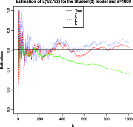
Figure 1: Estimation of $L(1/2,1/2)$ for the bivariate $\operatorname{Student}(2)$ law based on a sample of size 1000.

One can check from Figure 1 that the empirical estimator $\hat{L}_{k}$ behaves fairly well in terms of bias for small values of $k$. Besides, the bias is efficiently corrected by the two estimators $\accentset{\circ}{L}_{k}$ and $\tilde{L}_{k}$. Since the bias almost vanishes along the range of $k$, one can think about reducing the variance through an aggregation in $k$ (via mean or median) of $\accentset{\circ}{L}_{k}$ or $\tilde{L}_{k}$. This leads us to consider the two following estimators:

$$\accentset{\circ}{L}_{\mathrm{agg}} := \operatorname{Median}(\accentset{\circ}{L}_{k},k=1,\ldots,\kappa_{n}),$$

$$\tilde{L}_{\mathrm{agg}} := \operatorname{Median}(\tilde{L}_{k},k=1,\ldots,\kappa_{n}),$$

where $n$ is the sample size and $\kappa_{n}$ is an appropriate fraction of $n$. Their performance will be compared to those of the family $\{\hat{L}_{k},k=1,\ldots,n-1\}$. Simplified notation $\{\hat{L}_{k},k\}$ will be used instead of $\{\hat{L}_{k},k=1,\ldots,n-1\}$. Because any s.t.d.f. $L$ satisfies $\max(t,1-t)\leq L(1-t,t)\leq 1$, the competitors have been corrected so that they satisfy the same inequalities.

Remark 10.

If $\kappa_{n}$ satisfies the condition imposed on $k_{n}$ in Theorems 3 and 4, then the aggregated estimators $\accentset{\circ}{L}_{\mathrm{agg}}$ and $\tilde{L}_{\mathrm{agg}}$ would inherit the asymptotic properties of $\accentset{\circ}{L}_{k}$ and $\tilde{L}_{k}$. Indeed, all the estimators jointly converge, since they are based on a single process.

Remark 11.

In the following simulation study, $\kappa_{n}$ is arbitrarily fixed to $n-1$. Such a choice is open to criticism since it does not satisfy the theoretical assumptions mentioned in the previous remark. But it is motivated here by the fact that the bias happened to be efficiently corrected, even for very large values of $k$, as already illustrated on Figure 1. Note, however, that such a choice would not be systematically the right one. In presence of more complex models such as mixtures, $\kappa_{n}$ should not exceed the size of the subpopulation with heaviest tail. To illustrate this point, take, for example, the bivariate c.d.f. $F=pG+(1-p)H$, where $G$ is the c.d.f. of the bivariate $\operatorname{BPII}(3)$ model, and $H$ is the uniform c.d.f. on $[0,1]^{2}$. Then the s.t.d.f. is $L(x,y)=x+y-(1/x+1/y)^{-1}$, and only $p\%$ of the data belong to the targeted domain of attraction, so $\kappa_{n}$ should not exceed $pn$.

Classical criteria of quality of an estimator $\hat{\theta}$ of $\theta$ are the absolute bias (ABias) and the mean square error (MSE) defined by

$$\operatorname{ABias} = \frac{1}{N}\sum_{i=1}^{N}\bigl{|}\hat{\theta}^{(i)}-\theta\bigr{|},$$

$$\operatorname{MSE} = \frac{1}{N}\sum_{i=1}^{N}\bigl{(}\hat{\theta}^{(i)}-\theta\bigr{)}^{2},$$

where $N$ is the number of replicates of the experiment and $\hat{\theta}^{(i)}$ is the estimate from the $i$th sample. Note that what we call Abias is also referred as MAE (for Mean Absolute Error) in the literature. Figure 2 plots these criteria in the estimation of $L(1/2,1/2)$ for the bivariate $\operatorname{Student}(2)$ model when $n=1000$ and $N=200$.

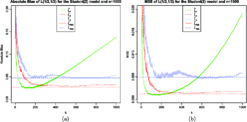
Figure 2: (a) ABias, (b) MSE for the estimation of $L(1/2,1/2)$ in the bivariate $\operatorname{Student}(2)$ model when $n=1000$ as a function of $k$.

Figure 2 exhibits the strong dependence of the behavior of $\hat{L}_{k}$ in terms of $k$, as well as the efficiency of the bias correction procedures. The estimator $\accentset{\circ}{L}_{k}$ given by (15) outperforms the estimator $\tilde{L}_{k}$ defined by (17), no matter the value of $k$. Moreover, the ABias and MSE curves associated to $\accentset{\circ}{L}_{k}$ almost reach the minimum of those of $\hat{L}_{k}$. Finally, the aggregated version $\accentset{\circ}{L}_{\mathrm{agg}}$ answers surprisingly well to the estimation problem of the s.t.d.f. $L$. First, its performance is similar to the best reachable from the original estimator $\hat{L}_{k}$. Second, it gets rid of the delicate choice of a threshold $k$ (or would at least simplify this choice; see Remark 11). These comparisons have also been made for five other models obtained from Section 4. The results are very similar to the ones obtained for the bivariate $\operatorname{Student}(2)$ distribution and are therefore not presented.

5.2 Comparisons in terms of $L^{1}$-error for $L$

The comparisons are now handled not only at a single point, but for the whole function using an $L^{1}$-error defined as follows:

$$\frac{1}{T+1}\sum_{t=1}^{T}\biggl{|}\hat{L}\biggl{(}1-\frac{t}{T},\frac{t}{T}\biggr{)}-L\biggl{(}1-\frac{t}{T},\frac{t}{T}\biggr{)}\biggr{|},$$ (21)

where $T$ is the size of the subdivision of $[0,1]$. Figure 3 gives the boxplots based on $N=100$ realizations of $\accentset{\circ}{L}_{\mathrm{agg}},\tilde{L}_{\mathrm{agg}}$ and $\{\hat{L}_{k},k\}$ for $T=30$ in the case of six bivariate models:

• First row: Cauchy and $\operatorname{Student}(2)$ models;

• Second row: $\operatorname{BPII}(3)$ model and Symmetric logistic model with $s=1/3$;

• Third row: Archimax model with logistic generator $L(x,y)=(x^{2}+y^{2})^{1/2}$ and mixed generator $L(x,y)=(x^{2}+y^{2}+xy)/(x+y)$.

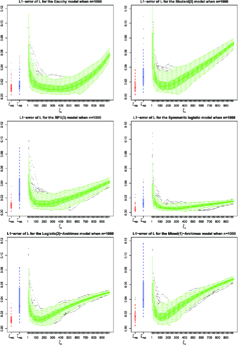
Figure 3: Boxplot of the $L^{1}$-error of function $L$ for the estimators $\accentset{\circ}{L}_{\mathrm{agg}},\tilde{L}_{\mathrm{agg}}$ and $\{\hat{L}_{k},k\}$. First row: bivariate Cauchy model (left) and bivariate $\operatorname{Student}(2)$ model (right). Second row: bivariate $\operatorname{BPII}(3)$ model (left) and bivariate Symmetric logistic model (right). Third row: bivariate Archimax model with logistic (left) and mixed generator (right).

As already observed in Figure 2, the estimator $\accentset{\circ}{L}_{\mathrm{agg}}$ is again very competitive compared to the best element of $\{\hat{L}_{k},k\}$, no matter the choice of model. Recall that the value of $k$ leading to the best $\hat{L}_{k}$ depends crucially on the model and is consequently unknown in practice, which invites any users to apply this new procedure.

The estimator $\tilde{L}_{\mathrm{agg}}$ is definitely less competitive compared to $\accentset{\circ}{L}_{\mathrm{agg}}$. Given these results we will not pursue with the $\tilde{L}_{\mathrm{agg}}$ estimator in the rest of this paper, and will focus our attention on the behavior of $\accentset{\circ}{L}_{\mathrm{agg}}$.

5.3 Comparisons between $\accentset{\circ}{L}_{\mathrm{agg}}$, a convex version of $\accentset{\circ}{L}_{\mathrm{agg}}$, and Peng’s estimator

A natural step is now to compare the performance of our best estimator $\accentset{\circ}{L}_{\mathrm{agg}}$ with an existing competitor, recently introduced by Peng (2010). In his work, Peng provides a data-driven method which chooses the threshold via estimating a s.t.d.f. Another interesting task is to compare $\accentset{\circ}{L}_{\mathrm{agg}}$ with a convexified version of itself, since any s.t.d.f. is a convex function; see, for example, Beirlant et al. [(2004), Section 8.2.2] or de Haan and Ferreira [(2006), Section 6.1.5]. Note that a general convexification procedure has been proposed in dimension 2 by Fils-Villetard, Guillou and Segers (2008); see also some alternative suggestions in Bücher, Dette and Volgushev (2011).

In order to take maximal advantage from this simulation study, the three different models implemented have been considered in two versions for each: the first model is the Gaussian one, simulated with Pearson’s correlation coefficient $\pm 0.5$. The Gaussian model is a particular case of elliptical distributions (see Section 4.2), which illustrates the asymptotic independent situation; cf. Remark 4. The second model is the bivariate Symmetric logistic one, introduced in Section 4.4, with two different strengths of dependence (close to independence on the left column, stronger dependence on the right column). The third model is the bivariate Student family, introduced in Sections 4.1 and 4.2 as a particular case. Two strengths of dependence have also been chosen, close to asymptotic independence on the left column and stronger dependence on the right column.

Our results, summarized in Figure 4, will thus exhibit in particular how the performance in the estimation of the s.t.d.f. depends on the distance to the asymptotic independence case. The $y$-axis scale has been fixed for all the six cases so that one can measure that the estimation of the s.t.d.f. is a more ambitious problem under asymptotic independence. However, our estimator $\accentset{\circ}{L}_{\mathrm{agg}}$ has still nice properties when comparing it to the empirical estimator $\hat{L}_{k}$.

The convex version $\accentset{\circ}{L}_{\mathrm{aggc}}$ performs quite equivalently as $\accentset{\circ}{L}_{\mathrm{agg}}$. A reason for this is that by construction our estimator is actually not far from a convex function. So balancing the cost of convexifying with the benefit in the performance motivates the simple use of $\accentset{\circ}{L}_{\mathrm{agg}}$.

Finally, regarding Peng’s estimator $\hat{L}_{P}$, one observes that this estimator is an interesting alternative to the original family $\{\hat{L}_{k},k\}$, which, however, never outperforms our proposal.

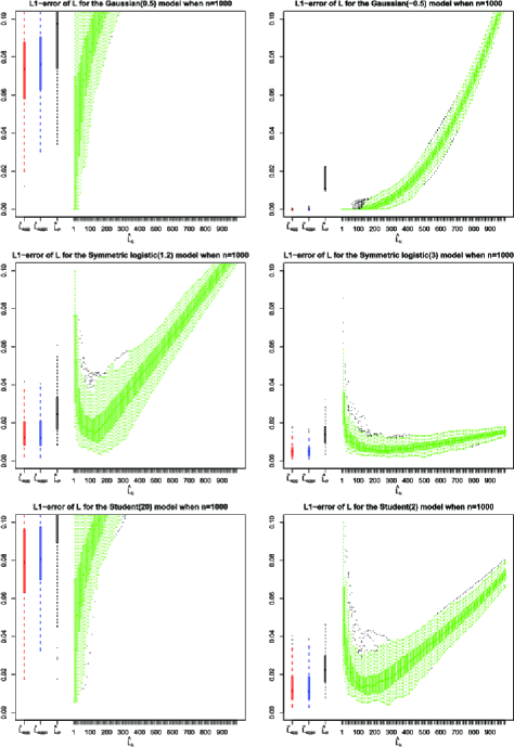
Figure 4: Boxplot of the $L^{1}$-error of function $L$ for the estimators $\accentset{\circ}{L}_{\mathrm{agg}},\accentset{\circ}{L}_{\mathrm{aggc}},\hat{L}_{P}$ and $\{\hat{L}_{k},k\}$. First row: bivariate Normal model with correlation $\tau$: $\tau=0.5$ (left) and $\tau=-0.5$ (right). Second row: bivariate Symmetric logistic$(s)$ model: $s=1/1.2$ (left) and $s=1/3$ (right). Third row: bivariate $\operatorname{Student}(\nu)$ model: $\nu=20$ (left) and $\nu=2$ (right).

5.4 Estimating a failure probability

Let us illustrate in this subsection the question of estimating an arbitrarily chosen failure probability $P(X>10^{4}$ or $Y>2\cdot 10^{4})$, where $(X,Y)$ comes from the $\operatorname{BPII}(3)$ model, so that $P(X>10^{4}$ or $Y>2\cdot 10^{4})=0.00011665$. Samples of size $n=1000$ are considered. Thus empirical estimation will be useless for evaluating the probability of exceeding such extreme values for $X$ or $Y$, and an extrapolation based on extreme value theory is thus needed.

First assume that it is known that the margins are standard Pareto. This probability can be approximated by

$$P\bigl{(}X>10^{4}\mbox{ or }Y>2\cdot 10^{4}\bigr{)}\simeq\bigl{(}10^{-4}+5\cdot 10^{-5}\bigr{)}L(2/3,1/3),$$

which naturally comes from (1), the projection on the simplex and the homogeneity of $L$. Estimating the unknown parameter $L(2/3,1/3)$ with our candidate $\accentset{\circ}{L}_{\mathrm{agg}}$ and the original family $\{\hat{L}_{k},k\}$ gives several boxplots (based on 500 replicates) that are presented in Figure 5. The comparison of these estimates is again favorable to $\accentset{\circ}{L}_{\mathrm{agg}}$.

Figure 5: Boxplot (based on 500 replicates) for the estimation of $P(X>10^{4}$ or $Y>2\cdot 10^{4})$ when $(X,Y)$ is drawn from the $\operatorname{BPII}(3)$ model with sample size $n=1000$ and assuming margins to be known.

Remark 12.

We also investigated the possible use of a second-order term in the approximation of the probability $P(X>10^{4}$ or $Y>2\cdot 10^{4})$, making use of the following estimators

$$\bigl{(}10^{-4}+5\cdot 10^{-5}\bigr{)}\accentset{\circ}{L}_{\mathrm{agg}}\biggl{(}\frac{2}{3},\frac{1}{3}\biggr{)}+\biggl{(}\frac{k}{n}\biggr{)}^{\hat{\rho}}\bigl{(}10^{-4}+5\cdot 10^{-5}\bigr{)}^{1-\hat{\rho}}\hat{\Delta}_{k,2^{-1/\hat{\rho}}}\biggl{(}\frac{2}{3},\frac{1}{3}\biggr{)}.$$

The results were so similar to those obtained in Figure 5 that we chose to skip them.

Second, when the margins are not assumed to be known, the estimation of $p_{1}=1-F_{1}(10^{4})$ and $p_{2}=1-F_{2}(2\cdot 10^{4})$ can be reached by the POT method [see, e.g., Beirlant et al. (2004), Section 7.4] for several values of a threshold. After the study of mean residual life plots and quantile plots, the thresholds have been fixed to be $X_{n-k,n}$ and $Y_{n-k,n}$ for $k=200$. The POT estimates deduced with these thresholds are, respectively, denoted by $\hat{p}_{1}$ and $\hat{p}_{2}$. The probability $P(X>10^{4}$ or $Y>2\cdot 10^{4})$ is then approximated by

$$P\bigl{(}X>10^{4}\mbox{ or }Y>2\cdot 10^{4}\bigr{)}\simeq(\hat{p}_{1}+\hat{p}_{2})L\biggl{(}\frac{\hat{p}_{1}}{\hat{p}_{1}+\hat{p}_{2}},\frac{\hat{p}_{2}}{\hat{p}_{1}+\hat{p}_{2}}\biggr{)}.$$

Estimating on each repetition the unknown parameter $L(\hat{p}_{1}/(\hat{p}_{1}+\hat{p}_{2}),\hat{p}_{2}/(\hat{p}_{1}+\hat{p}_{2}))$ with our candidate $\accentset{\circ}{L}_{\mathrm{agg}}$ and the original family $\{\hat{L}_{k},k\}$ gives several boxplots (based on 500 replicates) presented in Figure 6.

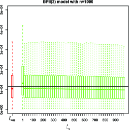
Figure 6: Boxplot (500 replicates) of the estimation of $P(X>10^{4}$ or $Y>2\cdot 10^{4})$ when $(X,Y)$ is drawn from the $\operatorname{BPII}(3)$ model with sample size $n=1000$ and estimating margins by POT method.

It seems clear that the uncertainty on the margins $F_{1}$ and $F_{2}$ has much more influence than that of the s.t.d.f. $L$. Such findings corroborate previous studies; see, for example, Bruun and Tawn (1998) and de Haan and Sinha (1999).

5.5 $Q$-curves

Another nice representation of a function of several variables is through its level sets. In the case of the function $L$, it consists of looking (for any positive real $c$) at sets of the form $\{(x,y)\in\mathbb{R}_{+}^{2},L(x,y)\leq c\}$. From homogeneity property, it is characterized by

$$Q:=\bigl{\{}(x,y)\in\mathbb{R}_{+}^{2},L(x,y)\leq 1\bigr{\}}.$$

Following de Haan and Ferreira [(2006), page 245], the boundary of this set can be written as

$$\partial Q=\bigl{\{}\bigl{(}b(\theta)\cos\theta,b(\theta)\sin\theta\bigr{)}:b(\theta)=\bigl{(}L(\cos\theta,\sin\theta)\bigr{)}^{-1},\theta\in[0,\pi/2]\bigr{\}}.$$

The estimation of $\partial Q$ is naturally obtained by replacing $L$ by any estimator, and this is done here for the estimators $\accentset{\circ}{L}_{\mathrm{agg}}$ and $\{\hat{L}_{k},k\}$. Figure 7 (left) exhibits the bias phenomenon (as $k$ increases) induced by $\hat{L}_{k}$ in the estimation of the $Q$-curve. The bias factor on $\hat{L}_{k}$ is illustrated with $k=50,k=100$ and $k=800$. The correction of the bias with $\accentset{\circ}{L}_{\mathrm{agg}}$ is effective. As in the previous section, the comparison of the different estimators is provided in terms of a global criterium based on the $L^{1}$-norm, given by

$$\frac{\pi}{2(T+1)}\sum_{t=0}^{T}\biggl{|}\hat{b}\biggl{(}\frac{\pi t}{2T}\biggr{)}-b\biggl{(}\frac{\pi t}{2T}\biggr{)}\biggr{|}\biggl{\{}\cos\biggl{(}\frac{\pi t}{2T}\biggr{)}+\sin\biggl{(}\frac{\pi t}{2T}\biggr{)}\biggr{\}}.$$

Figure 8 displays the boxplots of this measure, based on $N=100$ realizations and for $T=30$ under the six bivariate models given in the previous section.

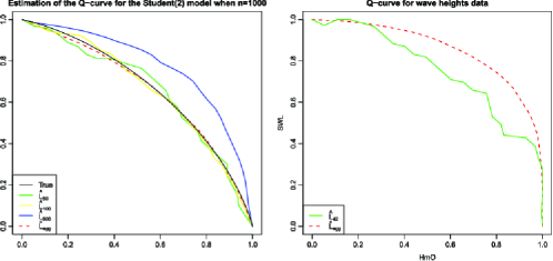
Figure 7: Left: Estimation of the $Q$-curve for the bivariate $\operatorname{Student}(2)$ law based on a sample of size 1000. Right: Estimated $Q$-curve for the wave heights data introduced in de Haan and Ferreira (2006).

The estimation of the $Q$-curve based on the original estimator $\hat{L}_{k}$ is strongly sensitive to the choice of $k$: the bias (resp., the variability) is an increasing (resp., decreasing) function of $k$. The performances of $\accentset{\circ}{L}_{\mathrm{agg}}$ is similar to that of the best $\hat{L}_{k}$, which is unknown in practice. These features corroborate the conclusions drawn in Section 5.2.

To close this section, let us illustrate the $Q$-curve estimation on the wave heights data set of de Haan and Ferreira (2006), page 207. As explained therein, wave height (HmO) and still water level (SWL) have been recorded during 828 storm events on the Dutch coast. The analogous Figure 7.2 from de Haan and Ferreira (2006) is reported in Figure 7 (right). Even if the two curves are not so close, the conclusion remains the same: the estimated boundary is concave, which indicates that the high values of the two variables are dependent.

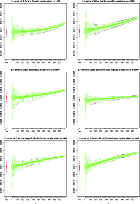
Figure 8: Boxplot of the $L^{1}$-error of $Q$-curve for the estimators $\accentset{\circ}{L}_{\mathrm{agg}}$ and $\{\hat{L}_{k},k\}$. First row: bivariate Cauchy model (left) and bivariate $\operatorname{Student}(2)$ model (right). Second row: bivariate $\operatorname{BPII}(3)$ model (left) and bivariate Symmetric logistic model (right). Third row: bivariate Archimax model with logistic (left) and mixed generator (right).

6 Estimation of second-order components $\rho$ and $M$

In this section, we focus on the estimation of the function $M$ coming from the second-order condition (– ‣ 2) and on the estimation of its homogeneity parameter $1-\rho$.

6.1 Second-order parameter $\rho$

A possible way to estimate $\rho$ is to use on each margin one of the techniques developed in the univariate setting; see, for example, Gomes, de Haan and Peng (2002) or Ciuperca and Mercadier (2010). Other methods make use of the multivariate structure of the data; see, for example, Peng (2010) and also Goegebeur and Guillou (2013) in a slightly different framework. The construction described here takes likewise advantage of the multivariate information of the sample. With this purpose, the following proposition shows that a variable of interest is the ratio of two terms $\hat{\Delta}_{k,a}$, defined by (11).

Proposition 5

Assume that the conditions of Proposition 1 are fulfilled and fix positive real numbers $r$ and $a\in(0,1)$. Assume moreover that the function $M$ never vanishes except on the axes. Then, as $n$ tends to infinity, for every $\varepsilon>0$ and $T>0$,

$$\sup_{\varepsilon\leq x_{1},\ldots,x_{d}\leq T}\biggl{|}\frac{\hat{\Delta}_{k,a}(r{\mathbf{x}})}{\hat{\Delta}_{k,a}({\mathbf{x}})}-r^{1-\rho}\biggr{|}\stackrel{{\scriptstyle\mathbb{P}}}{{\longrightarrow}}0.$$

Remark 13.

If the requirement that the function $M$ is either positive, or negative in the positive quadrant does not hold, one could consider the integral of $(\hat{\Delta}_{k,a}({\mathbf{x}}))^{2}$ over the set $\{{\mathbf{x}}=(x_{1},\ldots,x_{d})$ s.t. $x_{1}^{2}+\cdots+x_{d}^{2}=1\}$ and prove a result like Lemma 7 for this statistic. Then the integral of $M^{2}$ appears in the denominator in Proposition 5 instead of $M$ itself, and the sign of $M$ does not matter. This will be part of a future work.

A family of consistent estimators of the parameter $\rho$ can be derived from Proposition 5.

$$\hat{\rho}_{k,a,r}({\mathbf{x}}):=\biggl{(}1-\frac{1}{\log r}\log\biggl{|}\frac{\hat{\Delta}_{k,a}(r{\mathbf{x}})}{\hat{\Delta}_{k,a}({\mathbf{x}})}\biggr{|}\biggr{)}\wedge 0.$$ (22)

The following property can be obtained from the asymptotic expansion given in Proposition 2.

Proposition 6

Assume that the conditions of Proposition 2 are fulfilled, and fix positive real numbers $r$ and $a\in(0,1)$. Consider the estimator of $\rho$ defined by (22). Assume moreover that the function $M$ never vanishes except on the axes. Then, as $n$ tends to infinity,

$$\sqrt{k}\alpha\biggl{(}\frac{n}{k}\biggr{)}\bigl{\{}\hat{\rho}_{k,a,r}({\mathbf{x}})-\rho\bigr{\}}\stackrel{{\scriptstyle{d}}}{{\longrightarrow}}\hat{Z}_{\rho,a,r}({\mathbf{x}}),$$

in $D([\varepsilon,T]^{d})$ for every $\varepsilon>0$ and $T>0$, with

$$\hat{Z}_{\rho,a,r}({\mathbf{x}}):=\frac{a^{-1}Z_{L}(a{\mathbf{x}})-Z_{L}({\mathbf{x}})}{(a^{-\rho}-1)M({\mathbf{x}})\log r}-\frac{a^{-1}Z_{L}(ra{\mathbf{x}})-Z_{L}(r{\mathbf{x}})}{(a^{-\rho}-1)M({\mathbf{x}})r^{1-\rho}\log r}.$$

Figure 9 illustrates the finite sample behavior of this estimator of $\rho$ for a collection of bivariate models introduced in Section 4, for which the true value of $\rho$ is equal to $-$1.

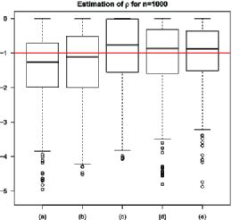
Figure 9: Boxplot of 500 estimations of $\rho$ given by (22) using samples of size 1000 drawn from six models: (a) $\operatorname{Student}(2)$; (b) $\operatorname{BPII}(3)$; (c) Symmetric Logistic with $s=1/3$; (d) Archimax model with logistic generator with $s=1/2$; (e) Archimax model with mixed generator. Red line indicates the true value of $\rho=-1$.

These boxplots show that the estimator performs reasonably well in median, no matter the choice of model, but the uncertainty is rather important. Fortunately this seems from simulation studies to have only minor influence on the estimation of $L$.

6.2 Second-order function $M$

Recall that from (12) the asymptotic bias of $\hat{L}_{k,a}({\mathbf{x}})$ is given by $\alpha(\frac{n}{k})a^{-\rho}M({\mathbf{x}})$. In order to circumvent an estimation of the term $\alpha(n/k)$, a renormalization is needed, focusing, for instance, on the estimation of $M({\mathbf{x}})/M({\mathbf{1}/2})$ where ${\mathbf{1}/2}=(1/2,\ldots,1/2)$. Thanks to (13), this ratio can be consistently estimated by

$$\frac{\hat{\Delta}_{k,a}({\mathbf{x}})}{\hat{\Delta}_{k,a}({\mathbf{1}/2})}$$

as soon as $k$ is a well-chosen intermediate sequence. The asymptotic normality can also be derived from analogous arguments to those used in the proof of Proposition 6. Details are not presented here for the sake of simplicity.

Figure 10 summarizes the behavior of the estimator of the curve $t\mapsto M(t,1-t)/M(1/2,1/2)$ through boxplots of the $L^{1}$-error, defined as in (21). We observe from this figure that the best estimation is reached for large values of $k$. This feature does not depend on the degree of asymptotic dependence in the Symmetric logistic model, nor on the strength of the bias of the original estimator $\hat{L}_{k}$ detected on Figure 3. These graphs confirm that the asymptotic bias is remarkably well estimated for large values of $k$. This helps to understand why the bias subtraction is accurate for large or very large choices of $k$, as also commented in Section 5.1.

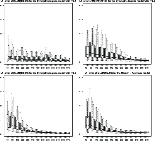
Figure 10: Boxplot of the $L^{1}$-error of $M(\cdot)/M(1/2,1/2)$-curve. First row: bivariate logistic model with $s=0.1$ (left) and with $s=0.5$ (right). Second row: bivariate logistic model with $s=0.9$ (left) and bivariate Archimax with mixed generator (right).

7 Concluding comments

This paper deals with the estimation of the extremal dependence structure in a multivariate context. Focusing on the s.t.d.f., the empirical counterpart is the nonparametric reference. A common feature when modeling extreme events is the delicate choice of the number of observations used in the estimation, and it spoils the good performance of this estimator. The aim of this paper has been to correct the asymptotic bias of the empirical estimator, so that the choice of the threshold becomes less sensitive. Two asymptotically unbiased estimators have been proposed and studied, both theoretically and numerically. The estimator defined in Section 3.2 proves to outperform the original estimator, whatever the model considered. Its aggregated version defined in Section 5.1 appears as a worthy candidate to estimate the s.t.d.f.

8 Proofs

Proof of Proposition 1 Denote by $U^{(j)}_{i}$ the uniform random variables $U^{(j)}_{i}=1-F_{j}(X^{(j)}_{i})$ for $j=1,\ldots,d$. Introducing

$$V_{k}({\mathbf{x}})=\frac{1}{k}\sum_{i=1}^{n}\mathbh{1}_{\{U^{(1)}_{i}\leq kx_{1}/n~{}\mathrm{or}~{}\ldots~{}\mathrm{or}~{}U^{(d)}_{i}\leq kx_{d}/n\}}$$

allows us to rewrite $\hat{L}_{k}$ as the following:

$$\hat{L}_{k}({\mathbf{x}})=V_{k}\biggl{(}\frac{n}{k}U^{(1)}_{[kx_{1}],n},\ldots,\frac{n}{k}U^{(d)}_{[kx_{d}],n}\biggr{)}.$$

Write

$$\hat{L}_{k}({\mathbf{x}})-L({\mathbf{x}})$$

$$\qquad=V_{k}\biggl{(}\frac{n}{k}U^{(1)}_{[kx_{1}],n},\ldots,\frac{n}{k}U^{(d)}_{[kx_{d}],n}\biggr{)}$$

$$\quad\qquad{}-\frac{n}{k}\bigl{[}1-F\bigl{\{}F_{1}^{-1}\bigl{(}1-U^{(1)}_{[kx_{1}],n}\bigr{)},\ldots,F_{d}^{-1}\bigl{(}1-U^{(d)}_{[kx_{d}],n}\bigr{)}\bigr{\}}\bigr{]}$$

$$\quad\qquad{}+\frac{n}{k}\bigl{[}1-F\bigl{\{}F_{1}^{-1}\bigl{(}1-U^{(1)}_{[kx_{1}],n}\bigr{)},\ldots,F_{d}^{-1}\bigl{(}1-U^{(d)}_{[kx_{d}],n}\bigr{)}\bigr{\}}\bigr{]}$$

$$\quad\qquad{}-L\biggl{(}\frac{n}{k}U^{(1)}_{[kx_{1}],n},\ldots,\frac{n}{k}U^{(d)}_{[kx_{d}],n}\biggr{)}$$

$$\quad\qquad{}+L\biggl{(}\frac{n}{k}U^{(1)}_{[kx_{1}],n},\ldots,\frac{n}{k}U^{(d)}_{[kx_{d}],n}\biggr{)}-L({\mathbf{x}}),$$

and denote $A_{1,k}({\mathbf{x}})$ [resp., $A_{2,k}({\mathbf{x}})$ and $A_{3,k}({\mathbf{x}})$] the first line (resp., second and third lines) of the right-hand side.

Applying de Haan and Ferreira [(2006), Proposition 7.2.3] leads to

$$\sqrt{k}A_{1,k}({\mathbf{x}})\stackrel{{\scriptstyle d}}{{\to}}W_{L}({\mathbf{x}}),$$

in $D([0,T]^{d})$ for every $T>0$ and for any intermediate sequence, where $W_{L}$ is a continuous centered Gaussian process with covariance structure specified in Proposition 2. Due to the Skorohod construction we can write

$$\sup_{0\leq x_{1},\ldots,x_{d}\leq T}\bigl{|}\sqrt{k}A_{1,k}({\mathbf{x}})-W_{L}({\mathbf{x}})\bigr{|}\to 0\qquad\mbox{a.s.},$$ (23)

which implies, since $\sqrt{k}\alpha(n/k)\to\infty$,

$$\sup_{0\leq x_{1},\ldots,x_{d}\leq T}\biggl{|}\frac{A_{1,k}({\mathbf{x}})}{\alpha(n/k)}\biggr{|}=O_{\mathbb{P}}\biggl{(}\frac{1}{\sqrt{k}\alpha(n/k)}\biggr{)}.$$

Again for any intermediate sequence, the proof of de Haan and Ferreira [(2006), Theorem 7.2.2] ensures the convergence for $j=1,\ldots,d$

$$\sup_{x\in[0,T]}\biggl{|}\sqrt{k}\biggl{(}\frac{n}{k}U^{(j)}_{[kx],n}-x\biggr{)}+W_{L}(x{\mathbf{e}}_{j})\biggr{|}\to 0\qquad\mbox{a.s.},$$ (24)

and finally

$$\sup_{0\leq x_{1},\ldots,x_{d}\leq T}\Biggl{|}\sqrt{k}A_{3,k}({\mathbf{x}})+\sum_{j=1}^{d}W_{L}(x_{j}{\mathbf{e}}_{j})\partial_{j}L({\mathbf{x}})\Biggr{|}\to 0\qquad\mbox{a.s.}$$ (25)

As previously, this yields

$$\sup_{0\leq x_{1},\ldots,x_{d}\leq T}\biggl{|}\frac{A_{3,k}({\mathbf{x}})}{\alpha(n/k)}\biggr{|}=O\biggl{(}\frac{1}{\sqrt{k}\alpha(n/k)}\biggr{)}.$$

Since the intermediate sequence satisfies $\sqrt{k}\alpha(\frac{n}{k})\to\infty$, it thus remains to prove that

$$\sup_{0\leq x_{1},\ldots,x_{d}\leq T}\biggl{|}\frac{A_{2,k}({\mathbf{x}})}{\alpha(n/k)}-M({\mathbf{x}})\biggr{|}\to 0\qquad\mbox{a.s.}$$

The second-order condition that holds uniformly on $[0,T]^{d}$ in (– ‣ 2) yields

$$\sup_{0\leq x_{1},\ldots,x_{d}\leq T}\biggl{|}\frac{A_{2,k}({\mathbf{x}})}{\alpha(n/k)}-M\biggl{(}\frac{n}{k}U^{(1)}_{[kx_{1}],n},\ldots,\frac{n}{k}U^{(d)}_{[kx_{d}],n}\biggr{)}\biggr{|}\to 0\qquad\mbox{a.s.}$$

Then the result follows from

$$\sup_{0\leq x_{1},\ldots,x_{d}\leq T}\biggl{|}M({\mathbf{x}})-M\biggl{(}\frac{n}{k}U^{(1)}_{[kx_{1}],n},\ldots,\frac{n}{k}U^{(d)}_{[kx_{d}],n}\biggr{)}\biggr{|}\to 0\qquad\mbox{a.s.},$$

which is obtained combining (24) and the continuity of the function $M$.

Proof of Proposition 2 We use the notation introduced in the proof of Proposition 1. Thanks to the Skorohod construction, we can start from (23). Combined with (25), it is sufficient to prove the convergence

$$\sup_{0\leq x_{1},\ldots,x_{d}\leq T}\biggl{|}\sqrt{k}\biggl{\{}A_{2,k}({\mathbf{x}})-\alpha\biggl{(}\frac{n}{k}\biggr{)}M({\mathbf{x}})\biggr{\}}\biggr{|}\to 0\qquad\mbox{a.s.}$$

Note that the third-order condition, the uniformity on $[0,T]^{d}$ of the convergence in (– ‣ 2) and the continuity of $N$ yield

$$A_{2,k}({\mathbf{x}})=\alpha\biggl{(}\frac{n}{k}\biggr{)}M\biggl{(}\frac{n}{k}U^{(1)}_{[kx_{1}],n},\ldots,\frac{n}{k}U^{(d)}_{[kx_{d}],n}\biggr{)}+O_{\mathbb{P}}\biggl{(}\alpha\biggl{(}\frac{n}{k}\biggr{)}\beta\biggl{(}\frac{n}{k}\biggr{)}\biggr{)}.$$

Thanks to (24) and to the existence of the first-order partial derivatives $\partial_{j}M$ $(j=1,\dots,d)$ of the function $M$, we have that

$$\sup_{0\leq x_{1},\ldots,x_{d}\leq T}\Biggl{|}\sqrt{k}\biggl{\{}M\biggl{(}\frac{n}{k}U^{(1)}_{[kx_{1}],n},\ldots,\frac{n}{k}U^{(d)}_{[kx_{d}],n}\biggr{)}-M({\mathbf{x}})\biggr{\}}$$

$$\hskip 121.0pt\qquad{}+\sum_{j=1}^{d}W_{L}(x_{j}{\mathbf{e}}_{j})\partial_{j}M({\mathbf{x}})\Biggr{|}$$

converges to 0 in probability, as $n$ tends to infinity. This implies that

$$\sup_{0\leq x_{1},\ldots,x_{d}\leq T}\biggl{|}\sqrt{k}\biggl{\{}A_{2,k}({\mathbf{x}})-\alpha\biggl{(}\frac{n}{k}\biggr{)}M({\mathbf{x}})\biggr{\}}\biggr{|}=O_{\mathbb{P}}\biggl{(}\biggl{|}\sqrt{k}\alpha\biggl{(}\frac{n}{k}\biggr{)}\beta\biggl{(}\frac{n}{k}\biggr{)}+\alpha\biggl{(}\frac{n}{k}\biggr{)}\biggr{|}\biggr{)},$$

which completes the proof, thanks to the choice of the intermediate sequence.

Proof of Theorem 3 Recall that $b=(a^{-\rho}+1)^{-1/\rho}$, and denote $\hat{b}=(a^{-\hat{\rho}}+1)^{-1/\hat{\rho}}$. Write

$$\accentset{\circ}{L}_{k,a,k_{\rho}}-L=\{\hat{L}_{k,a}-L\}+\{\hat{L}_{k}-L\}-\{\hat{L}_{k,\hat{b}}-L\},$$ (26)

which equals, thanks to (12) and under Skorohod’s construction,

$$\alpha\biggl{(}\frac{n}{k}\biggr{)}\bigl{(}a^{-\rho}+1\bigr{)}M({\mathbf{x}})+\frac{1}{\sqrt{k}}\bigl{(}a^{-1}Z_{L}(a{\mathbf{x}})+Z_{L}({\mathbf{x}})\bigr{)}$$

$$\quad{}-\alpha\biggl{(}\frac{n}{k}\biggr{)}\hat{b}^{-\rho}M({\mathbf{x}})-\frac{b^{-1}}{\sqrt{k}}Z_{L}(b{\mathbf{x}})+o\biggl{(}\frac{1}{\sqrt{k}}\biggr{)}$$

$$\qquad=\alpha\biggl{(}\frac{n}{k}\biggr{)}\bigl{(}\bigl{(}a^{-\rho}+1\bigr{)}-b^{-\rho}\bigr{)}M({\mathbf{x}})+\frac{1}{\sqrt{k}}\accentset{\circ}{Y}_{a}({\mathbf{x}})$$

$$\quad\qquad{}+\alpha\biggl{(}\frac{n}{k}\biggr{)}\bigl{(}b^{-\rho}-\hat{b}^{-\rho}\bigr{)}M({\mathbf{x}})+o\biggl{(}\frac{1}{\sqrt{k}}\biggr{)}$$

$$\qquad=\alpha\biggl{(}\frac{n}{k}\biggr{)}\bigl{(}\bigl{(}a^{-\rho}+1\bigr{)}-b^{-\rho}\bigr{)}M({\mathbf{x}})+\frac{1}{\sqrt{k}}\accentset{\circ}{Y}_{a}({\mathbf{x}})$$

$$\quad\qquad{}+\alpha\biggl{(}\frac{n}{k}\biggr{)}O_{\mathbb{P}}\biggl{(}\frac{1}{\sqrt{k_{\rho}}\alpha(n/k_{\rho})}\biggr{)}+o\biggl{(}\frac{1}{\sqrt{k}}\biggr{)}.$$

The first term is zero. Since both $k=o(k_{\rho})$ and $\alpha$ is regularly varying with negative index, the only the last term can be put into the term $o(\frac{1}{\sqrt{k}})$. Finally, the covariance function follows from the equality in law as processes between $Z_{L}(a{\mathbf{x}})$ and $\sqrt{a}Z_{L}({\mathbf{x}})$.

The proofs of Theorem 4 and Proposition 6 are based on the following auxiliary result.

Lemma 7

Assume that the conditions of Proposition 2 are fulfilled. Then for any positive real $r$, one has as $n$ tends to infinity,

$$\sqrt{k}\alpha\biggl{(}\frac{n}{k}\biggr{)}\biggl{\{}\frac{\hat{\Delta}_{k,a}(r{\mathbf{x}})}{\alpha(n/k)}-\bigl{(}a^{-\rho}-1\bigr{)}r^{1-\rho}M({\mathbf{x}})\biggr{\}}\stackrel{{\scriptstyle d}}{{\to}}a^{-1}Z_{L}(ra{\mathbf{x}})-Z_{L}(r{\mathbf{x}}),$$

in $D([0,T]^{d})$ for every $T>0$.

Proof of Lemma 7 Making use of the homogeneity of the function $L$, write

$$\hat{\Delta}_{k,a}(r{\mathbf{x}})=\bigl{\{}\hat{L}_{k,a}(r{\mathbf{x}})-L(r{\mathbf{x}})\bigr{\}}-\bigl{\{}\hat{L}_{k}(r{\mathbf{x}})-L(r{\mathbf{x}})\bigr{\}}.$$

Using the Skorohod construction, it follows from equations (8) and (12) that

$$\sup_{0\leq x_{1},\ldots,x_{d}\leq T/r}\biggl{|}\sqrt{k}\alpha\biggl{(}\frac{n}{k}\biggr{)}\biggl{\{}\frac{\hat{\Delta}_{k,a}(r{\mathbf{x}})}{\alpha(n/k)}-\bigl{(}a^{-\rho}-1\bigr{)}r^{1-\rho}M({\mathbf{x}})\biggr{\}}$$

$$\hskip 149.0pt{}-a^{-1}Z_{L}(ra{\mathbf{x}})+Z_{L}(r{\mathbf{x}})\biggr{|}$$

tends to 0 almost surely, as $n$ tends to infinity.

Proof of Theorem 4 Note that

$$\hat{L}_{k}({\mathbf{x}})\frac{\hat{\Delta}_{k_{\rho},a}(a{\mathbf{x}})}{\alpha(n/k_{\rho})}-\hat{L}_{k}(a{\mathbf{x}})\frac{\hat{\Delta}_{k_{\rho},a}({\mathbf{x}})}{\alpha(n/k_{\rho})}$$

$$\qquad=\hat{L}_{k}({\mathbf{x}})\biggl{(}\frac{\hat{\Delta}_{k_{\rho},a}(a{\mathbf{x}})}{\alpha(n/k_{\rho})}-a\frac{\hat{\Delta}_{k_{\rho},a}({\mathbf{x}})}{\alpha(n/k_{\rho})}\biggr{)}-a\frac{\hat{\Delta}_{k_{\rho},a}({\mathbf{x}})\hat{\Delta}_{k,a}({\mathbf{x}})}{\alpha(n/k_{\rho})}.$$

Under a Skorohod construction, Lemma 7 allows us to write the expansions of the terms $\hat{\Delta}_{k,a}({\mathbf{x}})$, $\hat{\Delta}_{k_{\rho},a}({\mathbf{x}})$ and $\hat{\Delta}_{k_{\rho},a}(a{\mathbf{x}})$, which implies on the one hand

$$\frac{\hat{\Delta}_{k_{\rho},a}(a{\mathbf{x}})}{\alpha(n/k_{\rho})}-a\frac{\hat{\Delta}_{k_{\rho},a}({\mathbf{x}})}{\alpha(n/k_{\rho})}$$

$$\qquad=a\bigl{(}a^{-\rho}-1\bigr{)}^{2}M({\mathbf{x}})$$

(27)

$$\qquad\quad{}+\frac{1}{\sqrt{k_{\rho}}\alpha(n/k_{\rho})}\bigl{\{}a^{-1}Z_{L}\bigl{(}a^{2}{\mathbf{x}}\bigr{)}-2Z_{L}(a{\mathbf{x}})+aZ_{L}({\mathbf{x}})\bigr{\}}$$

$$\quad\qquad{}+o\biggl{(}\frac{1}{\sqrt{k_{\rho}}\alpha(n/k_{\rho})}\biggr{)},$$

and

$$\frac{\hat{\Delta}_{k_{\rho},a}({\mathbf{x}})\hat{\Delta}_{k,a}({\mathbf{x}})}{\alpha(n/k_{\rho})} = \alpha(n/k)\bigl{(}a^{-\rho}-1\bigr{)}^{2}M^{2}({\mathbf{x}})$$

$${}+\bigl{(}a^{-\rho}-1\bigr{)}M({\mathbf{x}})\frac{a^{-1}Z_{L}(a{\mathbf{x}})-Z_{L}({\mathbf{x}})}{\sqrt{k}}$$

$${}+O_{\mathbb{P}}\biggl{(}\frac{\alpha(n/k)}{\sqrt{k_{\rho}}\alpha(n/k_{\rho})}+\frac{1}{\sqrt{k}\sqrt{k_{\rho}}\alpha(n/k_{\rho})}\biggr{)}+o\biggl{(}\frac{1}{\sqrt{k}}\biggr{)}$$

on the other hand, both uniformly for ${\mathbf{x}}\in[\varepsilon,T]^{d}$. Combining (8) and (8) with equation (8), one gets

$$\hat{L}_{k}({\mathbf{x}})\frac{\hat{\Delta}_{k_{\rho},a}(a{\mathbf{x}})}{\alpha(n/k_{\rho})}-\hat{L}_{k}(a{\mathbf{x}})\frac{\hat{\Delta}_{k_{\rho},a}({\mathbf{x}})}{\alpha(n/k_{\rho})}$$

$$\qquad=a\bigl{(}a^{-\rho}-1\bigr{)}^{2}M({\mathbf{x}})L({\mathbf{x}})+\frac{1}{\sqrt{k}}M({\mathbf{x}})\bigl{(}a^{-\rho}-1\bigr{)}\bigl{(}a^{1-\rho}Z_{L}({\mathbf{x}})-Z_{L}(a{\mathbf{x}})\bigr{)}$$

$$\quad\qquad{}+\frac{1}{\sqrt{k_{\rho}}\alpha(n/k_{\rho})}L({\mathbf{x}})\bigl{\{}a^{-1}Z_{L}\bigl{(}a^{2}{\mathbf{x}}\bigr{)}-2Z_{L}(a{\mathbf{x}})+aZ_{L}({\mathbf{x}})\bigr{\}}$$

$$\quad\qquad{}+o\biggl{(}\frac{1}{\sqrt{k}}\biggr{)}+o\biggl{(}\frac{1}{\sqrt{k_{\rho}}\alpha(n/k_{\rho})}\biggr{)}.$$

Since the last expression and equation (8) are, respectively, the numerator and denominator of $\tilde{L}_{k,k_{\rho},a}({\mathbf{x}})$, one obtains, after simplification,

$$\sqrt{k}\bigl{(}\tilde{L}_{k,k_{\rho},a}({\mathbf{x}})-L({\mathbf{x}})\bigr{)}=\frac{a^{-\rho}Z_{L}({\mathbf{x}})-a^{-1}Z_{L}(a{\mathbf{x}})}{a^{-\rho}-1}+o\biggl{(}\frac{\sqrt{k}}{\sqrt{k_{\rho}}\alpha(n/k_{\rho})}\biggr{)}+o(1),$$

since $M$ does not vanish by assumption. The choice of the sequences $k$ and $k_{\rho}$ allows us to conclude since $\sqrt{k}=O(\sqrt{k_{\rho}}\alpha(n/k_{\rho}))$.

Proof of Proposition 5 Applying Lemma 7, we have

$$\sup_{\varepsilon\leq x_{1},\ldots,x_{d}\leq T}\biggl{|}\frac{\hat{\Delta}_{k,a}({\mathbf{x}})}{\alpha(n/k)}-\bigl{(}a^{-\rho}-1\bigr{)}M({\mathbf{x}})\biggr{|}\stackrel{{\scriptstyle\mathbb{P}}}{{\longrightarrow}}0.$$ (29)

As a consequence,

$$\sup_{\varepsilon\leq x_{1},\ldots,x_{d}\leq T}\biggl{|}\frac{\hat{\Delta}_{k,a}(r{\mathbf{x}})}{\hat{\Delta}_{k,a}({\mathbf{x}})}-r^{1-\rho}\biggr{|}$$

$$\qquad=\sup_{\varepsilon\leq x_{1},\ldots,x_{d}\leq T}\biggl{|}\frac{\hat{\Delta}_{k,a}(r{\mathbf{x}})/\alpha(n/k)}{\hat{\Delta}_{k,a}({\mathbf{x}})/\alpha(n/k)}-r^{1-\rho}\biggr{|}$$

$$\qquad=O_{\mathbb{P}}\biggl{(}\sup_{\varepsilon\leq x_{1},\ldots,x_{d}\leq T}\biggl{|}\frac{\hat{\Delta}_{k,a}(r{\mathbf{x}})}{\alpha(n/k)}-r^{1-\rho}\frac{\hat{\Delta}_{k,a}({\mathbf{x}})}{\alpha(n/k)}\biggr{|}\biggr{)},$$

since $(a^{-\rho}-1)M({\mathbf{x}})\neq 0$ by assumption. Writing

$$\biggl{|}\frac{\hat{\Delta}_{k,a}(r{\mathbf{x}})}{\alpha(n/k)}-r^{1-\rho}\frac{\hat{\Delta}_{k,a}({\mathbf{x}})}{\alpha(n/k)}\biggr{|}$$

$$\qquad\leq\biggl{|}\frac{\hat{\Delta}_{k,a}(r{\mathbf{x}})}{\alpha(n/k)}-r^{1-\rho}\bigl{(}a^{-\rho}-1\bigr{)}M({\mathbf{x}})\biggr{|}$$

$$\quad\qquad{}+\biggl{|}r^{1-\rho}\bigl{(}a^{-\rho}-1\bigr{)}M({\mathbf{x}})-r^{1-\rho}\frac{\hat{\Delta}_{k,a}({\mathbf{x}})}{\alpha(n/k)}\biggr{|},$$

and using twice equation (29) leads to the conclusion.

Proof of Proposition 6 Define $Q_{k,a,r}({\mathbf{x}}):=\frac{\hat{\Delta}_{k,a}(r{\mathbf{x}})}{\hat{\Delta}_{k,a}({\mathbf{x}})}$. Lemma 7 used twice yields

$$\sqrt{k}\alpha\biggl{(}\frac{n}{k}\biggr{)}\bigl{(}Q_{k,a,r}({\mathbf{x}})-r^{1-\rho}\bigr{)}\stackrel{{\scriptstyle d}}{{\to}}-r^{1-\rho}\log r\hat{Z}_{\rho,a,r}({\mathbf{x}}),$$ (30)

where $\hat{Z}_{\rho,a,r}({\mathbf{x}})$ is defined in Proposition 6. Since $\hat{\rho}_{k,a,r}({\mathbf{x}})=1-\log(Q_{k,a,r}({\mathbf{x}}))/\log r$, the result follows straightforwardly from (30) and the Delta method.

References

- Abdous and Ghoudi (2005) {barticle}[mr] \bauthor\bsnmAbdous, \bfnmBelkacem\binitsB. and \bauthor\bsnmGhoudi, \bfnmKilani\binitsK. (\byear2005). \btitleNon-parametric estimators of multivariate extreme dependence functions. \bjournalJ. Nonparametr. Stat. \bvolume17 \bpages915–935. \biddoi=10.1080/10485250500336379, issn=1048-5252, mr=2192166 \bptokimsref\endbibitem
- Beirlant, Dierckx and Guillou (2011) {barticle}[mr] \bauthor\bsnmBeirlant, \bfnmJ.\binitsJ., \bauthor\bsnmDierckx, \bfnmG.\binitsG. and \bauthor\bsnmGuillou, \bfnmA.\binitsA. (\byear2011). \btitleBias-reduced estimators for bivariate tail modelling. \bjournalInsurance Math. Econom. \bvolume49 \bpages18–26. \biddoi=10.1016/j.insmatheco.2011.01.010, issn=0167-6687, mr=2811890 \bptokimsref\endbibitem
- Beirlant et al. (2004) {bbook}[mr] \bauthor\bsnmBeirlant, \bfnmJan\binitsJ., \bauthor\bsnmGoegebeur, \bfnmYuri\binitsY., \bauthor\bsnmTeugels, \bfnmJozef\binitsJ. and \bauthor\bsnmSegers, \bfnmJohan\binitsJ. (\byear2004). \btitleStatistics of Extremes: Theory and Applications. \bpublisherWiley, \blocationChichester. \biddoi=10.1002/0470012382, mr=2108013 \bptokimsref\endbibitem
- Bruun and Tawn (1998) {barticle}[author] \bauthor\bsnmBruun, \bfnmJ. T.\binitsJ. T. and \bauthor\bsnmTawn, \bfnmJ. A.\binitsJ. A. (\byear1998). \btitleComparison of approaches for estimating the probability of coastal flooding. \bjournalAppl. Statist. \bvolume47 \bpages405–423. \bptokimsref\endbibitem
- Bücher, Dette and Volgushev (2011) {barticle}[mr] \bauthor\bsnmBücher, \bfnmAxel\binitsA., \bauthor\bsnmDette, \bfnmHolger\binitsH. and \bauthor\bsnmVolgushev, \bfnmStanislav\binitsS. (\byear2011). \btitleNew estimators of the Pickands dependence function and a test for extreme-value dependence. \bjournalAnn. Statist. \bvolume39 \bpages1963–2006. \biddoi=10.1214/11-AOS890, issn=0090-5364, mr=2893858 \bptokimsref\endbibitem
- Caeiro, Gomes and Rodrigues (2009) {barticle}[mr] \bauthor\bsnmCaeiro, \bfnmFrederico\binitsF., \bauthor\bsnmGomes, \bfnmM. Ivette\binitsM. I. and \bauthor\bsnmRodrigues, \bfnmLígia Henriques\binitsL. H. (\byear2009). \btitleReduced-bias tail index estimators under a third-order framework. \bjournalComm. Statist. Theory Methods \bvolume38 \bpages1019–1040. \biddoi=10.1080/03610920802361415, issn=0361-0926, mr=2522545 \bptokimsref\endbibitem
- Cai, de Haan and Zhou (2013) {barticle}[mr] \bauthor\bsnmCai, \bfnmJuan-Juan\binitsJ.-J., \bauthor\bparticlede \bsnmHaan, \bfnmLaurens\binitsL. and \bauthor\bsnmZhou, \bfnmChen\binitsC. (\byear2013). \btitleBias correction in extreme value statistics with index around zero. \bjournalExtremes \bvolume16 \bpages173–201. \biddoi=10.1007/s10687-012-0158-x, issn=1386-1999, mr=3057195 \bptnotecheck related \bptokimsref\endbibitem
- Capéraà and Fougères (2000) {barticle}[mr] \bauthor\bsnmCapéraà, \bfnmPhilippe\binitsP. and \bauthor\bsnmFougères, \bfnmAnne-Laure\binitsA.-L. (\byear2000). \btitleEstimation of a bivariate extreme value distribution. \bjournalExtremes \bvolume3 \bpages311–329. \biddoi=10.1023/A:1012241624430, issn=1386-1999, mr=1870461 \bptokimsref\endbibitem
- Capéraà, Fougères and Genest (2000) {barticle}[mr] \bauthor\bsnmCapéraà, \bfnmPhilippe\binitsP., \bauthor\bsnmFougères, \bfnmAnne-Laure\binitsA.-L. and \bauthor\bsnmGenest, \bfnmChristian\binitsC. (\byear2000). \btitleBivariate distributions with given extreme value attractor. \bjournalJ. Multivariate Anal. \bvolume72 \bpages30–49. \biddoi=10.1006/jmva.1999.1845, issn=0047-259X, mr=1747422 \bptokimsref\endbibitem
- Ciuperca and Mercadier (2010) {barticle}[mr] \bauthor\bsnmCiuperca, \bfnmGabriela\binitsG. and \bauthor\bsnmMercadier, \bfnmCécile\binitsC. (\byear2010). \btitleSemi-parametric estimation for heavy tailed distributions. \bjournalExtremes \bvolume13 \bpages55–87. \biddoi=10.1007/s10687-009-0086-6, issn=1386-1999, mr=2593951 \bptokimsref\endbibitem
- Coles and Tawn (1991) {barticle}[mr] \bauthor\bsnmColes, \bfnmStuart G.\binitsS. G. and \bauthor\bsnmTawn, \bfnmJonathan A.\binitsJ. A. (\byear1991). \btitleModelling extreme multivariate events. \bjournalJ. Roy. Statist. Soc. Ser. B \bvolume53 \bpages377–392. \bidissn=0035-9246, mr=1108334 \bptokimsref\endbibitem
- de Haan and Ferreira (2006) {bbook}[mr] \bauthor\bparticlede \bsnmHaan, \bfnmLaurens\binitsL. and \bauthor\bsnmFerreira, \bfnmAna\binitsA. (\byear2006). \btitleExtreme Value Theory: An Introduction. \bpublisherSpringer, \blocationNew York. \biddoi=10.1007/0-387-34471-3, mr=2234156 \bptokimsref\endbibitem
- de Haan, Mercadier and Zhou (2014) {bmisc}[author] \bauthor\bparticlede \bsnmHaan, \bfnmL.\binitsL., \bauthor\bsnmMercadier, \bfnmC.\binitsC. and \bauthor\bsnmZhou, \bfnmC.\binitsC. (\byear2014). \bhowpublishedAdapting extreme value statistics to financial time series: Dealing with bias and serial dependence. Submitted. \bptokimsref\endbibitem
- de Haan and Resnick (1993) {barticle}[mr] \bauthor\bparticlede \bsnmHaan, \bfnmL.\binitsL. and \bauthor\bsnmResnick, \bfnmSidney I.\binitsS. I. (\byear1993). \btitleEstimating the limit distribution of multivariate extremes. \bjournalComm. Statist. Stochastic Models \bvolume9 \bpages275–309. \biddoi=10.1080/15326349308807267, issn=0882-0287, mr=1213072 \bptokimsref\endbibitem
- de Haan and Sinha (1999) {barticle}[mr] \bauthor\bparticlede \bsnmHaan, \bfnmLaurens\binitsL. and \bauthor\bsnmSinha, \bfnmAshoke Kumar\binitsA. K. (\byear1999). \btitleEstimating the probability of a rare event. \bjournalAnn. Statist. \bvolume27 \bpages732–759. \biddoi=10.1214/aos/1018031214, issn=0090-5364, mr=1714710 \bptokimsref\endbibitem
- Demarta and McNeil (2005) {barticle}[author] \bauthor\bsnmDemarta, \bfnmS.\binitsS. and \bauthor\bsnmMcNeil, \bfnmA. J.\binitsA. J. (\byear2005). \btitleThe t copula and related copulas. \bjournalInt. Stat. Rev. \bvolume73 \bpages111–129. \bptokimsref\endbibitem
- Einmahl, de Haan and Sinha (1997) {barticle}[mr] \bauthor\bsnmEinmahl, \bfnmJohn H. J.\binitsJ. H. J., \bauthor\bparticlede \bsnmHaan, \bfnmLaurens\binitsL. and \bauthor\bsnmSinha, \bfnmAshoke Kumar\binitsA. K. (\byear1997). \btitleEstimating the spectral measure of an extreme value distribution. \bjournalStochastic Process. Appl. \bvolume70 \bpages143–171. \biddoi=10.1016/S0304-4149(97)00065-3, issn=0304-4149, mr=1475660 \bptokimsref\endbibitem
- Einmahl, Krajina and Segers (2008) {barticle}[mr] \bauthor\bsnmEinmahl, \bfnmJohn H. J.\binitsJ. H. J., \bauthor\bsnmKrajina, \bfnmAndrea\binitsA. and \bauthor\bsnmSegers, \bfnmJohan\binitsJ. (\byear2008). \btitleA method of moments estimator of tail dependence. \bjournalBernoulli \bvolume14 \bpages1003–1026. \biddoi=10.3150/08-BEJ130, issn=1350-7265, mr=2543584 \bptokimsref\endbibitem
- Einmahl, Krajina and Segers (2012) {barticle}[mr] \bauthor\bsnmEinmahl, \bfnmJohn H. J.\binitsJ. H. J., \bauthor\bsnmKrajina, \bfnmAndrea\binitsA. and \bauthor\bsnmSegers, \bfnmJohan\binitsJ. (\byear2012). \btitleAn -estimator for tail dependence in arbitrary dimensions. \bjournalAnn. Statist. \bvolume40 \bpages1764–1793. \biddoi=10.1214/12-AOS1023, issn=0090-5364, mr=3015043 \bptokimsref\endbibitem
- Fils-Villetard, Guillou and Segers (2008) {barticle}[mr] \bauthor\bsnmFils-Villetard, \bfnmAmélie\binitsA., \bauthor\bsnmGuillou, \bfnmArmelle\binitsA. and \bauthor\bsnmSegers, \bfnmJohan\binitsJ. (\byear2008). \btitleProjection estimators of Pickands dependence functions. \bjournalCanad. J. Statist. \bvolume36 \bpages369–382. \biddoi=10.1002/cjs.5550360303, issn=0319-5724, mr=2456011 \bptokimsref\endbibitem
- Fraga Alves, de Haan and Lin (2003) {barticle}[mr] \bauthor\bsnmFraga Alves, \bfnmM. I.\binitsM. I., \bauthor\bparticlede \bsnmHaan, \bfnmL.\binitsL. and \bauthor\bsnmLin, \bfnmTao\binitsT. (\byear2003). \btitleEstimation of the parameter controlling the speed of convergence in extreme value theory. \bjournalMath. Methods Statist. \bvolume12 \bpages155–176. \bidissn=1066-5307, mr=2025356 \bptokimsref\endbibitem
- Goegebeur and Guillou (2013) {barticle}[mr] \bauthor\bsnmGoegebeur, \bfnmYuri\binitsY. and \bauthor\bsnmGuillou, \bfnmArmelle\binitsA. (\byear2013). \btitleAsymptotically unbiased estimation of the coefficient of tail dependence. \bjournalScand. J. Stat. \bvolume40 \bpages174–189. \biddoi=10.1111/j.1467-9469.2012.00800.x, issn=0303-6898, mr=3024038 \bptokimsref\endbibitem
- Gomes, de Haan and Peng (2002) {barticle}[mr] \bauthor\bsnmGomes, \bfnmM. Ivette\binitsM. I., \bauthor\bparticlede \bsnmHaan, \bfnmLaurens\binitsL. and \bauthor\bsnmPeng, \bfnmLiang\binitsL. (\byear2002). \btitleSemi-parametric estimation of the second order parameter in statistics of extremes. \bjournalExtremes \bvolume5 \bpages387–414. \biddoi=10.1023/A:1025128326588, issn=1386-1999, mr=2002125 \bptokimsref\endbibitem
- Gomes, de Haan and Rodrigues (2008) {barticle}[mr] \bauthor\bsnmGomes, \bfnmM. Ivette\binitsM. I., \bauthor\bparticlede \bsnmHaan, \bfnmLaurens\binitsL. and \bauthor\bsnmRodrigues, \bfnmLígia Henriques\binitsL. H. (\byear2008). \btitleTail index estimation for heavy-tailed models: Accommodation of bias in weighted log-excesses. \bjournalJ. R. Stat. Soc. Ser. B. Stat. Methodol. \bvolume70 \bpages31–52. \bidissn=1369-7412, mr=2412630 \bptokimsref\endbibitem
- Guillotte, Perron and Segers (2011) {barticle}[mr] \bauthor\bsnmGuillotte, \bfnmSimon\binitsS., \bauthor\bsnmPerron, \bfnmFrançois\binitsF. and \bauthor\bsnmSegers, \bfnmJohan\binitsJ. (\byear2011). \btitleNon-parametric Bayesian inference on bivariate extremes. \bjournalJ. R. Stat. Soc. Ser. B. Stat. Methodol. \bvolume73 \bpages377–406. \biddoi=10.1111/j.1467-9868.2010.00770.x, issn=1369-7412, mr=2815781 \bptokimsref\endbibitem
- Hall and Welsh (1985) {barticle}[mr] \bauthor\bsnmHall, \bfnmPeter\binitsP. and \bauthor\bsnmWelsh, \bfnmA. H.\binitsA. H. (\byear1985). \btitleAdaptive estimates of parameters of regular variation. \bjournalAnn. Statist. \bvolume13 \bpages331–341. \biddoi=10.1214/aos/1176346596, issn=0090-5364, mr=0773171 \bptokimsref\endbibitem
- Huang (1992) {bmisc}[author] \bauthor\bsnmHuang, \bfnmX.\binitsX. (\byear1992). \bhowpublishedStatistics of bivariate extremes. Ph.D. thesis, Erasmus Univ. Rotterdam, Tinbergen Institute Research series No. 22. \bptokimsref\endbibitem
- Joe (1990) {barticle}[mr] \bauthor\bsnmJoe, \bfnmHarry\binitsH. (\byear1990). \btitleFamilies of min-stable multivariate exponential and multivariate extreme value distributions. \bjournalStatist. Probab. Lett. \bvolume9 \bpages75–81. \biddoi=10.1016/0167-7152(90)90098-R, issn=0167-7152, mr=1035994 \bptokimsref\endbibitem
- Joe, Smith and Weissman (1992) {barticle}[mr] \bauthor\bsnmJoe, \bfnmHarry\binitsH., \bauthor\bsnmSmith, \bfnmRichard L.\binitsR. L. and \bauthor\bsnmWeissman, \bfnmIshay\binitsI. (\byear1992). \btitleBivariate threshold methods for extremes. \bjournalJ. Roy. Statist. Soc. Ser. B \bvolume54 \bpages171–183. \bidissn=0035-9246, mr=1157718 \bptokimsref\endbibitem
- Kotz, Balakrishnan and Johnson (2000) {bbook}[mr] \bauthor\bsnmKotz, \bfnmSamuel\binitsS., \bauthor\bsnmBalakrishnan, \bfnmN.\binitsN. and \bauthor\bsnmJohnson, \bfnmNorman L.\binitsN. L. (\byear2000). \btitleContinuous Multivariate Distributions: Models and Applications, \bedition2nd ed. \bseriesWiley Series in Probability and Statistics: Applied Probability and Statistics \bvolume1. \bpublisherWiley, \blocationNew York. \biddoi=10.1002/0471722065, mr=1788152 \bptokimsref\endbibitem
- Krajina (2012) {barticle}[mr] \bauthor\bsnmKrajina, \bfnmAndrea\binitsA. (\byear2012). \btitleA method of moments estimator of tail dependence in meta-elliptical models. \bjournalJ. Statist. Plann. Inference \bvolume142 \bpages1811–1823. \biddoi=10.1016/j.jspi.2012.01.020, issn=0378-3758, mr=2903392 \bptokimsref\endbibitem
- Ledford and Tawn (1996) {barticle}[mr] \bauthor\bsnmLedford, \bfnmAnthony W.\binitsA. W. and \bauthor\bsnmTawn, \bfnmJonathan A.\binitsJ. A. (\byear1996). \btitleStatistics for near independence in multivariate extreme values. \bjournalBiometrika \bvolume83 \bpages169–187. \biddoi=10.1093/biomet/83.1.169, issn=0006-3444, mr=1399163 \bptokimsref\endbibitem
- Ledford and Tawn (1997) {barticle}[mr] \bauthor\bsnmLedford, \bfnmAnthony W.\binitsA. W. and \bauthor\bsnmTawn, \bfnmJonathan A.\binitsJ. A. (\byear1997). \btitleModelling dependence within joint tail regions. \bjournalJ. Roy. Statist. Soc. Ser. B \bvolume59 \bpages475–499. \biddoi=10.1111/1467-9868.00080, issn=0035-9246, mr=1440592 \bptokimsref\endbibitem
- Peng (1998) {barticle}[mr] \bauthor\bsnmPeng, \bfnmL.\binitsL. (\byear1998). \btitleAsymptotically unbiased estimators for the extreme-value index. \bjournalStatist. Probab. Lett. \bvolume38 \bpages107–115. \biddoi=10.1016/S0167-7152(97)00160-0, issn=0167-7152, mr=1627906 \bptokimsref\endbibitem
- Peng (2010) {barticle}[mr] \bauthor\bsnmPeng, \bfnmLiang\binitsL. (\byear2010). \btitleA practical way for estimating tail dependence functions. \bjournalStatist. Sinica \bvolume20 \bpages365–378. \bidissn=1017-0405, mr=2640699 \bptokimsref\endbibitem
- Resnick (1986) {barticle}[mr] \bauthor\bsnmResnick, \bfnmSidney I.\binitsS. I. (\byear1986). \btitlePoint processes, regular variation and weak convergence. \bjournalAdv. in Appl. Probab. \bvolume18 \bpages66–138. \biddoi=10.2307/1427239, issn=0001-8678, mr=0827332 \bptokimsref\endbibitem
- Tawn (1988) {barticle}[mr] \bauthor\bsnmTawn, \bfnmJonathan A.\binitsJ. A. (\byear1988). \btitleBivariate extreme value theory: Models and estimation. \bjournalBiometrika \bvolume75 \bpages397–415. \biddoi=10.1093/biomet/75.3.397, issn=0006-3444, mr=0967580 \bptokimsref\endbibitem