KYUSHU-HET-153

Abstract

We study dynamics of a cosmic string in a metastable brane configuration in Type IIA string theory. We first discuss a decay process of the cosmic string via a fuzzy brane (equivalently bubble/string bound state) by neglecting gravitational corrections in ten-dimension. We find that depending on the strength of the magnetic field induced on the bubble, the decay rate can be either larger or smaller than that of $O(4)$ symmetric bubble. Then, we investigate gravitational corrections to the fuzzy brane by using the extremal black $NS$-five brane solution, which makes the lifetime of the metastable state longer.

1 Introduction

Remarkable progress on string compactification may suggest us that the potential of string theories has a complicated structure and admits a large number of metastable vacua [1]. This string landscape, if it is true, would open up a new avenue for cosmology at the early stage of the universe. One of interesting dynamics in the string landscape is transition between various metastable vacua (see [2, 3, 4, 5] and references therein for earlier works). It is fascinating to think that transitions between vacua occur several times at the early stage and eventually the system arrives at the present universe with small cosmological constant. In this sense, studies of the lifetime of various vacua would be important subject. However due to lack of full knowledge of the string landscape, analytic studies on this subject are quite hard. So it would be useful to take a limit in which we can neglect gravitational corrections and to extract lessons on longevity of vacua from “limited” string landscape.

In the first paper [6], the authors studied inhomogenious vacuum decay via a stringy monopole. The authors showed that dielectric branes [7], which are bound states of a spherical $D5$ brane and a $D3$ brane, are key objects for decays of false vacua. It can be either unstable or metastable depending on the magnetic flux originating from the dissolving $D3$ brane in the $D5$ brane. As emphasized, the lower energy vacuum filling in the bubble offers a force to enlarge the radius of the spherical bubble and in fact, a stable fuzzy monopole with finite size (dielectric brane) was formed without using background flux [7, 8] nor angular momentum [9]. This is a new mechanism for creating stable fuzzy branes. Also, when the induced magnetic flux is large enough, the fuzzy monopole becomes unstable and expands its radius without bound. This is remarkable because the lifetime of the false vacuum becomes drastically shorter due to the decay of the unstable monopole. A decay process exploiting a fuzzy brane was initially studied in [10] where anti-$D3$ branes create a fuzzy $NS5$ brane, and later extended to various decay channels in related models [11]. Recent progress on this subject can be seen in [12] and references therein.

The idea of the inhomogeneous decay of false vacua via solitons was initially pointed out by [13, 14, 15]. Then, in [16, 17, 18], applications to phenomenological model building were discussed in the context of field theories. Our first paper [6] can be regarded as the first realization of this idea in string theories. In this paper, we would like to go a step further toward including gravitational effects. To this goal, we use a brane configuration in Type IIA string theory. In this context, it is relatively easy to incorporate the gravitational corrections by means of replacing an $NS$-five brane with the extremal black-brane solution, which allows us to evaluate the decay rate explicitly within the validity of the brane-limit. This is one of advantages to use a metastable brane configuration to get an insight into decay processes under gravitational effects.

The plan of this paper is as follows. In section 2, we review a metastable configuration in Type IIA string theory [19, 20, 21, 22]. In section 3, after reviewing a cosmic string existing in the metastable configuration along the lines of [23], we investigate stability of a dielectric brane which is a bound state of the string and a tube-like domain wall connecting the false and true vacua. In section 4, we discuss gravitational corrections to the decay process affected by the $NS$-five brane background. Section 5 is devoted to conclusions and discussions.

2 Set-up of brane configuration

In this section, we quickly review false and true vacua in brane configuration in Type IIA string theory discussed in [19, 20, 21, 22]. See [24] for a recent review on supersymmetry (SUSY) breaking vacua in string theories. In contrast to the work [6], the potential barrier between false and true vacua is very shallow, because it is created by higher order corrections. Hence, estimation of the decay rate of the false vacuum is carried out by triangle approximation [25] rather than thin-wall approximation [26], which leads to a slightly different conclusion from [6]: existence of a soliton does not necessarily make the lifetime of false vacuum shorter.

To begin with, let us review the supersymmetry breaking brane configuration [19, 20, 21, 22]. It is useful to introduce the following parametrization for internal space,

$$v=x^{4}+ix^{5},\qquad w=x^{8}+ix^{9},\qquad y=x^{6}.$$ (2.1)

Consider three $NS$-five branes extending in $v$ or $w$ directions. We refer to branes placed at $(y,v)=(y_{1},0)$, $(y,v)=(y_{1}+\Delta y,\Delta v)$ and $(y,w)=(y_{NS},0)$ as $NS_{1}$, $NS_{2}$ and $NS_{3}$ branes respectively. There are $N$ $D4$ branes stretched between the $NS_{2}$ and $NS_{3}$ branes. Also, $n$ tilted $D4$ branes are stretched between the $NS_{1}$ and $NS_{2}$ branes.

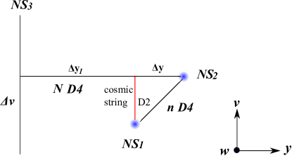
Figure 1: A metastable brane configuration. As we will discuss in the next section, a $D2$ brane filling $x^{4}$ direction in $v$ plane corresponds to a cosmic string [23]. We define $\Delta y_{1}=y_{1}-y_{NS}$ for later convenience.

If we take the field theory limit, $l_{s}\to 0$, while keeping the following quantities finite,

$$h^{2}={8\pi^{2}g_{s}l_{s}\over\Delta y},\qquad\mu^{2}={\Delta v\over 16\pi^{3}g_{s}l_{s}^{3}},$$ (2.2)

this brane configuration can be interpreted as the $U(N)$ gauge theory with $N+n$ flavors and the following superpotential [27],

$$W_{\rm mag}=hq^{j}_{\alpha}\Phi^{i}_{j}\tilde{q}_{i}^{\alpha}-h\mu^{2}\Phi_{i}^{i},$$ (2.3)

where $\Phi$ is a singlet in the $U(N)$ gauge group. $i,j$ run from $1$ to $N+n$ and $\alpha$ is the color index. The vacuum energy in this configuration is

$$V_{\rm meta}=n|h\mu^{2}|^{2}.$$ (2.4)

Note that in this brane configuration, there is an $n\times n$ matrix $X$ of massless fields corresponding to the positions of the tilted $D4$ branes in the $w$ direction. This is a flat direction of this brane configuration at tree level. Hereafter we assume $n=1$ for the sake of simplicity. As discussed in [27, 28], there are two kinds of corrections which lift the flat direction. One is the Coleman-Weinberg (CW) potential generated by open strings connecting between the $N$ $D4$ and the $n$ tilted $D4$ branes. The other comes from the gravitational effect originating from $NS_{3}$ brane as we will discuss in section 4 in detail. The second contribution becomes relevant in the so-called brane limit where $g_{s}$ is very small but $l_{s}$ is finite. In [27, 28], the explicit calculation has been done,

$$V_{\rm correction} = \left({\ln 4-1\over 8\pi^{2}}N|h^{2}\mu|^{2}+{\Delta v\over\sqrt{(\Delta y)^{2}+(\Delta v)^{2}}}{l_{s}\over y_{NS}^{2}}\right){\rm Tr}X^{\dagger}X+\cdots$$ (2.5)

$$= K_{0}|h^{2}\mu|^{2}{\rm Tr}X^{\dagger}X+\cdots,$$

where we have defined

$$K_{0}\equiv{\ln 4-1\over 8\pi^{2}}N+{\Delta v\over\sqrt{(\Delta y)^{2}+(\Delta v)^{2}}}{l_{s}\over y_{NS}^{2}}{1\over|h^{2}\mu|^{2}}.$$ (2.6)

The first term in the parenthesis is dominant when $\mu\ll 1/l_{s}$.

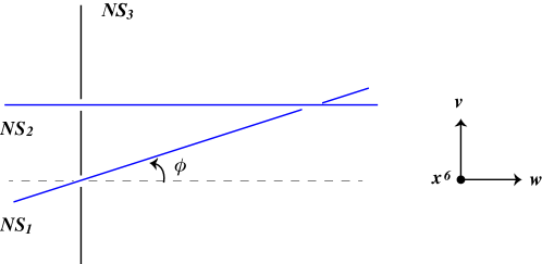
Figure 2: The $NS_{1}$ brane is rotated by the angle $\phi$ in $w-v$ plane.

Now, let us engineer a SUSY preserving vacuum within the validity of this brane configuration without disturbing metastability. To do this, we slightly rotate the $NS_{1}$ brane by an angle $\phi$ in $(v,w)$ space. See figure 2. This rotation can be interpreted as adding the mass term of the moduli $X$ to the superpotential [19, 20, 21, 22],

$$\Delta W={1\over 2}h^{2}\mu_{\phi}{\rm Tr}X^{2},\qquad\mu_{\phi}={\tan\phi\over 8\pi^{2}g_{s}l_{s}}.$$ (2.7)

From the second expression in (2.7), we see that the new parameter $\mu_{\phi}$ is described by geometric data. Adding this correction to the superpotential (2.3), we find that the SUSY preserving and breaking vacua are placed at

$$X_{\rm SUSY}={\mu^{2}\over h\mu_{\phi}},\qquad X_{\rm meta}\simeq{\mu_{\phi}\over hK_{0}}.$$ (2.8)

From this, we see that the metastable vacuum is slightly shifted away from the origin. For later convenience, we define

$$\Delta_{8}\equiv(X_{\rm SUSY}-X_{\rm meta})l_{s}^{2},\qquad x_{0}^{8}\equiv X_{\rm meta}l_{s}^{2}.$$ (2.9)

Finally, let us review the decay rate of the metastable vacuum. As in ISS model [27], we use the triangle approximation [25] for the evaluation since the depth of the potential near the metastable vacuum is shallow but the distance from the metastable vacuum to the SUSY vacuum is large. The transition can take place by creating a bubble in Minkowski space-time which corresponds to the domain wall $D4$ brane filling a subspace in the internal space. The tension of the bubble is

$$T_{\rm DW}=T_{D4}S_{2},\qquad S_{2}=\Delta_{8}\sqrt{(\Delta_{4})^{2}+(\Delta y)^{2}}\simeq\Delta_{8}\Delta_{4},$$ (2.10)

where $S_{2}$ is the area in $(x^{4},x^{6},x^{8})$ filled by the $D4$ brane. For the sake of simplicity, we assume $\Delta y\ll\Delta_{4}$ below. The lifetime of the metastable vacuum is estimated by using the results in [25],

$$\Gamma\sim\exp\left(-B_{\rm triangle}\right),\qquad B_{\rm triangle}={2\pi^{2}\over 3}{(\Delta X)^{4}\over\Delta V}.$$

In our setup, the distance between two vacua is given by $\Delta X\simeq X_{\rm SUSY}$. The vacuum energy of the metastable vacuum is

$$\Delta V=V_{\rm peak}-V_{\rm meta}=N_{\rm peak}h^{2}\mu^{4}.$$ (2.11)

Finding the peak of the potential is not a trivial task because in our approximation, this analysis is reliable only when

$$h\mu^{2}\gg h^{2}\mu_{\phi}X.$$ (2.12)

In other words, the behavior of the potential near the origin is reliable. However, the peak of the potential places far away from the origin, which makes the estimation slightly hard. Here, we roughly assume the place of the peak is given by the geometric mean of two vacua, $X_{\rm peak}={\mu\over h\sqrt{K_{0}}}$, and estimate the value of $N_{\rm peak}$. Plugging the geometric mean back into the potential, we get $V_{\rm peak}\sim 2V_{\rm meta}$, so we obtain $N_{\rm peak}=1$. Hereafter, we simply assume that $N_{\rm peak}$ is an ${\cal O}(1)$ constant.

3 Fuzzy cosmic string (without gravity)

3.1 Dielectric tube-like brane nucleated from cosmic string

Now we are ready to discuss vacuum decay via a dielectric brane. In the metastable vacuum there exists a string-like object firstly pointed out by [23]. A $D2$ brane connecting the $NS_{1}$ brane and the horizontal $D4$ branes can be seen as a string in Minkowski space-time. See figure 1. So the domain wall $D4$ brane and the $D2$ brane are stretching to the same directions in the internal space. Note that there is a small displacement in $x^{8}$ direction that requires the extra cost to form the bound state of $D2$/$D4$ branes [33]. However, since we mainly assume that $X_{\rm SUSY}\gg X_{\rm meta}$ this energy cost can be negligible in our argument below. By the $D2$ brane dissolving, the total energy of the system is given by

$$E_{\rm total} = \sqrt{\left(T_{D4}S_{2}2\pi RL\right)^{2}+\left(n_{D2}T_{D2}\Delta_{8}L\right)^{2}}-\Delta V\pi R^{2}L$$ (3.1)

$$= {4\pi T_{\rm DW}^{2}L\over\Delta V}\left[\sqrt{r^{2}+b^{2}}-r^{2}\right]$$

$$\equiv {4\pi T_{\rm DW}^{2}L\over\Delta V}E_{\rm num},$$

where we have defined,

$$r={\Delta V\over 2T_{\rm DW}}R,\qquad b={n_{D2}T_{D2}\Delta_{8}\Delta V\over 4\pi T_{\rm DW}^{2}}.$$ (3.2)

Here, we have neglected the constant contribution from the homogeneous vev of the metastable vacuum because it does not play any role for dynamics. Also, we assumed that the $D2$/$D4$ brane forms a loop with the size $L$. In figure 3, we show the energy behavior. We find that there is no metastable dielectric brane with finite size. The instability condition on the string-like object is

$$b\geq{1\over 2}~{},\qquad{\rm(unstable)}.$$ (3.3)

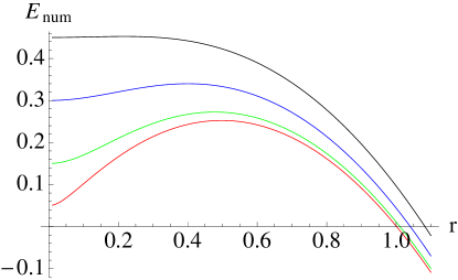
Figure 3: $b=1/20,3/20,6/20,9/20$ for the red, green, blue and black lines

3.2 Decay rate of metastable string

Now we have learnt the cosmic string can be either unstable or metastable depending on $b$. For the parameter region $b\geq{1/2}$, even if the vacuum has enough longevity, the vacuum decay via dielectric brane brings about the instant phase transition. On the other hand, when the condition $b<1/2$ is satisfied, the decay process is caused by an $O(2)$ symmetric instanton. In this subsection, we investigate this decay process. Fortunately, we can proceed the study basically along the lines of [30, 31, 32]. We assume the following embedding function,

$$X^{0}=t,\quad X^{1}=z,\quad X^{2}=R(t,z)\cos\theta,\quad X^{3}=R(t,z)\sin\theta,$$

$$X^{4}=x^{4},\quad(0\leq x^{4}\leq\Delta_{4}),\quad X^{8}=x^{8},\quad(x_{0}^{8}\leq x^{8}\leq x_{0}^{8}+\Delta_{8}),$$ (3.4)

where $X^{5,6,7,9}$ are constant. Since the cosmic string is along $z$ and $x^{4}$ directions in the $D4$ brane coordinates, the dissolved $D2$-brane yields the magnetic field in the $(\theta,x^{8})$ directions, Hence, the low energy effective action can be obtained by turning on $B\equiv 2\pi\alpha^{\prime}F_{\theta x^{8}}$. Exploiting the following expression,

$$\partial_{\alpha}X^{\mu}\partial_{\beta}X_{\mu}+2\pi\alpha^{\prime}F_{\alpha\beta}=\begin{pmatrix}-1+\dot{R}^{2}&\dot{R}R^{\prime}&0&0&0\\ \dot{R}R^{\prime}&1+R^{\prime 2}&0&0&0\\ 0&0&R^{2}&0&B\\ 0&0&0&1&0\\ 0&0&-B&0&1\end{pmatrix},$$ (3.5)

where $\alpha$ and $\beta$ are the indices of the world-sheet coordinates, the DBI action is given by

$$S=-T_{D4}\int d^{5}\xi\sqrt{(R^{2}+B^{2})(1-\dot{R}^{2}+R^{\prime 2})}+\int dt\,\pi R^{2}L\Delta V.$$ (3.6)

Below, for the sake of simplicity, we assume $R^{\prime}=0$. To estimate the decay rate, let us write down the Euclidean action,

$$S_{E}=\int d\tau\left[2\pi T_{\rm DW}L\sqrt{(R^{2}+B^{2})(1+\dot{R}^{2})}-\pi R^{2}L\Delta V\right],$$ (3.7)

where $T_{\rm DW}=T_{D4}\Delta_{4}\Delta_{8}$. It is useful to introduce the dimensionless parameters,

$$s={\Delta V\over 2T_{\rm DW}}\tau,\qquad r={\Delta V\over 2T_{\rm DW}}R,\qquad b={\Delta V\over 2T_{\rm DW}}B.$$ (3.8)

Then, the Euclidean action becomes

$$S_{E} = 2\pi\left({2T_{\rm DW}\over\Delta V}\right)^{2}T_{\rm DW}L\int ds\left[\sqrt{(r^{2}+b^{2})(1+\dot{r}^{2})}-r^{2}\right]$$ (3.9)

$$= {8\pi LT_{\rm DW}^{3}\over\Delta V^{2}}S_{\rm num}^{O(2)}.$$

The equation of motion can be described by the first order differential equation,

$$\sqrt{{r^{2}+b^{2}\over 1+\dot{r}^{2}}}-r^{2}=C,$$ (3.10)

where $C$ is the integration constant. From this expression, we can discuss the velocity of a solution, $\dot{r}$,

$$\dot{r}=\pm\sqrt{r^{2}+b^{2}-(C+r^{2})^{2}\over(C+r^{2})^{2}}.$$ (3.11)

Since the initial condition is $\dot{r}=0$ at the core of the string $r=0$, the solution of the equation should satisfy the following factorization condition,

$$r^{2}+b^{2}-(C+r^{2})^{2}=r(r_{\rm max}-r)(r^{2}+a_{1}r+a_{0}).$$ (3.12)

By solving this condition we find that $C=b$, $a_{0}=0$, $r_{\rm max}=a_{1}=\sqrt{1-2b}$. With this bounce solution, the velocity is written as follows,

$$\dot{r}=\pm{r\sqrt{r^{2}_{\rm max}-r^{2}}\over(b+r^{2})}.$$ (3.13)

Plugging this back into (3.9), we calculate the exponent of the decay rate,

$$B_{O(2)} = 2\cdot{8\pi LT_{\rm DW}^{3}\over\Delta V^{2}}\left(S^{O(2)}_{\rm num}(r_{\rm bounce})-S^{O(2)}_{\rm num}(0)\right)$$ (3.14)

$$= {16\pi LT_{\rm DW}^{3}\over\Delta V^{2}}\left[\int_{0}^{r_{\rm max}}dr{b+r^{2}\over r\sqrt{r_{\rm max}^{2}-r^{2}}}\left({r^{2}+b^{2}\over b+r^{2}}-r^{2}\right)-b\int_{0}^{r_{\rm max}}dr{b+r^{2}\over r\sqrt{r_{\rm max}^{2}-r^{2}}}\right]$$

$$= {16\pi LT_{\rm DW}^{3}\over\Delta V^{2}}\int_{0}^{r_{\rm max}}drr\sqrt{r_{\rm max}^{2}-r^{2}}$$

$$= {16\pi LT_{\rm DW}^{3}\over 3\Delta V^{2}}(1-2b)^{3\over 2}=B_{O(4)}l(1-2b)^{3\over 2},$$

where $l\equiv 2\left({2\over 3}\right)^{4}{\Delta V\over\pi T_{DW}}L$. Note that $B_{O(4)}$ is the bounce action of the thin-wall approximation [26]. Since we are neglecting the curvature effect of the torus, the size $L$ should be much larger than the string scale $l_{s}$, $L\gg l_{s}$. Thus, within the validity of our approximation we find $l>1$.

To estimate the decay rate, it is useful to rewrite $B_{\rm triangle}$ in terms of $B_{O(4)}$. Recalling that the domain wall tension is written by $\Delta X$, we obtain

$${B_{\rm triangle}\over B_{O(4)}}\equiv k_{0}={4\pi^{2}\over 9N_{\rm peak}}\left({\Delta V\over 3\pi(T_{D4}\Delta_{4}l_{s}^{2})^{2}}\right)^{2}<1.$$ (3.15)

The last inequality comes from the fact that the depth of the potential in the current setup is shallow and the triangle approximation is the dominant contribution. From (3.14) and (3.15), we find that there is the critical point where two bounce actions become equal,

$$k_{0}=l(1-2b_{\rm crit})^{3\over 2}.$$ (3.16)

As an illustration, we show a schematic behavior of the ratio of two bounce actions in figure 4. In the region $0\leq b<b_{\rm crit}$, since $B_{O(2)}>B_{\rm triangle}$, the decay via an $O(2)$ symmetric bubble is subdominant. On the other hand, In the region $b_{\rm crit}<b<{1\over 2}$, we see that $B_{O(2)}<B_{\rm triangle}$, so catalysis induced by the string plays an important role.

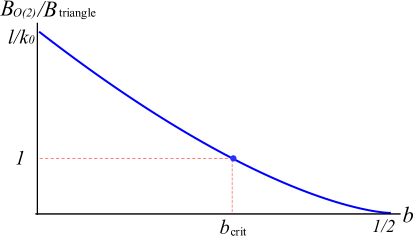
Figure 4: The ratio of two bounce actions for the case of parameter choice, $l>k_{0}$.

3.3 Adding fundamental string

Finally, let us briefly study effects of colliding fundamental strings to the fuzzy brane. First of all, we discuss the case when a fundamental string wraps in the $\theta$ direction, namely wraps on the smaller cycle of the torus. In this case, doing the same way as before, we obtain the Lagrangian written in terms of the electric density flux $D$ as follows:

$${S}=-\int dt\,\left[2\pi T_{\rm DW}L\sqrt{(1+D^{2})(R^{2}+B^{2})(1-\dot{R}^{2})}-\pi R^{2}L\Delta V\right].$$ (3.17)

By simply replacing the domain wall tension as $T_{\rm DW}\to T_{\rm DW}\sqrt{1+D^{2}}$, we can apply the analysis done in the subsection 3.2. Since the tension becomes large, stability of the dielectric brane enhances. Physical meaning of this effect is clear: wrapped fundamental strings try to shrink and generate forces making the radius of the dielectric brane small.

The other interesting situation is that fundamental strings are dissolving in the domain wall brane along the $x^{8}$ direction. In this case, by calculating the DBI action explicitly, we find again that the action, for $R^{\prime}=0$, becomes exactly the same as the one studied in [6]. The electric flux is along the $x^{8}$ direction while the magnetic flux is in $(\theta,x^{8})$ directions, the total action of the tube-like brane becomes

$$S=-\int dt\left[2\pi LT_{\rm DW}\sqrt{R^{2}(1-\dot{R}^{2}-E_{8}^{2})+B^{2}(1-\dot{R}^{2})}-\pi R^{2}L\Delta V\right].$$ (3.18)

Using the results shown in [6], we find that the critical value depends on the strength of the electric flux. The result is plotted in figure 5. Finally, when the fundamental string dissolves along the $z$-direction, we can easily obtain the decay rate by replacing $B^{2}\to B^{2}+D^{2}$.

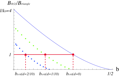
Figure 5: The ratio of two bounce actions for $l/k_{0}=4$. Blue and green dots correspond to $d=2/10$ and $d=1/10$. When $b>b_{\rm crit}$, decays through $O(2)$ symmetric instantons are dominant.

4 Gravitational corrections

In this section, we discuss gravitational interactions in ten-dimension between the branes and the fuzzy brane. As studied in [28], the interactions generate a non-negligible effective potential for light fields and modify the landscape of the potential. Here, we study dynamics of the fuzzy brane under such interactions. This is the first step to get insights into gravitational corrections for inhomogeneous vacuum decay in string landscape.

4.1 Stability of cosmic string corrected by gravity

At first, we review stability of the false vacuum under such gravitational interactions. The $NS_{1}$, $NS_{2}$ branes and the tilted $D4$ branes are mutually BPS, so there is no force between them. On the other hand, since the $NS_{3}$ brane and the tilted $D4$ branes are mutually non-BPS, they interact non-trivially, which leads to the most important correction in the following argument. When the distance of the $D4$-brane from the $NS_{3}$ brane is quite large, this correction can be treated as the classical background five-brane solution [28, 29]. We can take account of the gravitational correction to the DBI action by analyzing the motion of the $D4$ brane in the presence of this background. Also, the tilted $D4$ branes and the horizontal $D4$ branes are mutually non-BPS, so there is a force between them which has been already incorporated as loop corrections of open strings between them.

The classical solution of the $NS$-five brane discussed in [29] is

$$ds^{2}=dx_{\mu}dx^{\mu}+dvd\bar{v}+H(r_{\rm NS})[dy^{2}+(dx^{7})^{2}+dwd\bar{w}],$$

$$e^{2(\varphi-\varphi_{0})}=H(x^{n})$$ (4.1)

$$H_{lmn}=-\epsilon_{lmnp}\partial_{q}\varphi.$$ (4.2)

$H_{lmn}$ is the strength of the NS $B$ field, $dB_{2}$. The indices run $\mu,\nu=0,1,2,3$ and $l,m,n,p=6,7,8,9$. The exponential of dilaton, $e^{\varphi_{0}}$, is interpreted as the string coupling constant $g_{s}$. The harmonic function $H$ is given by

$$H(r_{\rm NS})=1+{l_{s}^{2}\over r^{2}_{\rm NS}},\qquad{\rm where}\quad r^{2}_{\rm NS}=(y-y_{NS})^{2}+(x^{7})^{2}+|w|^{2}.$$ (4.3)

As mentioned above, since the dominant gravitational correction comes from the $NS_{3}$ brane, so we apply this solution only to the $NS_{3}$ brane and study dynamics of the $n$ tilted $D4$ branes and the fuzzy $D4$ brane. By gravitational corrections, the minimum of the SUSY breaking vacuum shifts slightly. To see this, write down the DBI action of the tilted $D4$ brane in this background. The potential for the $D4$ brane becomes [28]

$$V={T_{4}\Delta y\over g_{s}}\left(\sqrt{1+{(2\pi)^{4}(l_{s}h\mu)^{2}\over H(r_{\rm NS})}}-1\right).$$ (4.4)

This depends on $w$, and we find that there is a force pulling the $D4$ brane back to the origin. When the $NS_{3}$ brane is far enough from the other $NS$ branes, $y_{NS}\to-\infty$, the energy of the metastable vacuum is given as the minimum of this potential plus the correction mentioned in the previous section, $V_{\rm correction}$. We do not need the actual value of this in the following discussion, then we formally write this minimum and the energy at the minimum as

$$w_{\rm meta}=x_{\rm meta},\qquad\Delta V={T_{4}\Delta y\over g_{s}}\left(\sqrt{1+{(2\pi)^{4}(l_{s}h\mu)^{2}\over H(x_{\rm meta})}}-1\right).$$ (4.5)

Here we have fixed the energy of the SUSY vacuum to be 0.

Now we have reviewed gravitational corrections to the metastable vacuum, we start to think gravitational corrections to the vacuum decay via the cosmic string. As in the previous section, suppose there is a string-like object corresponding to the $D2$ brane stretched between the $NS_{1}$ brane and the horizontal $D4$ branes, and assume that a tube-like domain wall connecting two vacua is induced by the string. The string on the top of the $D4$ brane is energetically unstable and dissolves into the $D4$ brane [33]. We investigate dynamics of the $D2$/$D4$ bound state. We take the embedding function of the $D4$ brane the same as in the previous section. In the background (4.2), the DBI action of the $D4$ brane becomes

$$\sqrt{-\det(\partial_{\alpha}X^{\mu}\partial_{\beta}X_{\mu}+2\pi\alpha^{\prime}F_{\alpha\beta})}=\sqrt{H(r_{\rm NS})R^{2}+B^{2}},$$ (4.6)

where we have assumed that the radius $R$ is constant along the string and time. We find the potential energy to be

$$E=\left(T_{D4}\Delta_{4}\Delta_{8}\right){1\over\Delta_{8}}\int dx^{8}\,2\pi L\sqrt{H(r_{\rm NS})R^{2}+B^{2}}-\pi R^{2}L\Delta V.$$ (4.7)

It is useful to introduce dimensionless variables,

$$x^{8}\equiv x_{\rm meta}\cdot q,\qquad\epsilon\equiv{x_{\rm meta}\over\Delta_{8}},\qquad L_{s}\equiv{l_{s}\over x_{\rm meta}},\qquad\Delta Y\equiv{\Delta y\over x_{\rm meta}}.$$ (4.8)

For the sake of simplicity, we assume that $x^{7}$ and $\Delta y$ dependences are negligible. So, we have $r^{2}_{\rm NS}=(\Delta y_{1})^{2}+(x^{8})^{2}$. By plugging these expressions, the energy function is written as follows:

$$E=2\pi T_{\rm DW}\left({2T_{\rm DW}\over\Delta V}\right)L\left[\epsilon\int_{1}^{1+1/\epsilon}dq\sqrt{\left(1+{L_{s}^{2}\over\Delta Y^{2}+q^{2}}\right)r^{2}+b^{2}}-r^{2}\right].$$ (4.9)

We have used the fact $x_{\rm SUSY}=x_{\rm meta}+\Delta_{8}$. As an illustration, we plot this potential in figure 6. Obviously, the potential barrier becomes higher by gravitational corrections, thus the metastable state is stabilized. This can be understood that a force generated by the black $NS$-five brane pulling back the domain wall $D4$ brane impedes the decay.

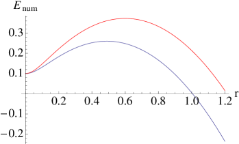
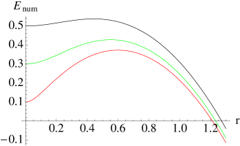
Figure 6: In the left panel. Red for $\Delta Y=5$, $L_{s}=5$, $b=1/10$, $\epsilon=1/10$. Blue corresponds to the case with $L_{s}=0$. In the right panel, $\Delta Y=5$, $L_{s}=5$, $\epsilon=1/10$ the red, green and black correspond to $b=1/10$, $3/10$ and $5/10$.

From this potential, we can read off the critical strength of the magnetic field that makes the fuzzy brane unstable. Differentiating $E$ with respect to $r$, we find that the local minimum exists at $r=0$, and the maximum at the radius satisfying the following condition,

$$\epsilon\int_{1}^{1+1/\epsilon}dq\left[{H\over\sqrt{Hr^{2}+b^{2}}}-2\right]=0.$$ (4.10)

In our assumption, the harmonic function is given by

$$H=1+{L_{s}^{2}\over\Delta Y^{2}+q^{2}}.$$ (4.11)

At the critical strength of the magnetic field these two points collide. This condition is written as

$$2b_{\rm unst}=\epsilon\int_{1}^{1+1/\epsilon}Hdq.$$ (4.12)

This integral is analytically solved and we find the critical value is described by

$$b_{\rm unst} = {1\over 2}+{\epsilon L_{s}^{2}\over 2\Delta Y}\left[\tan^{-1}\left({1\over\Delta Y}+{1\over\epsilon\Delta Y}\right)-\tan^{-1}\left({1\over\Delta Y}\right)\right]$$ (4.13)

$$= {1\over 2}+{\epsilon L_{s}^{2}\over 2\Delta Y}\tan^{-1}\left({\Delta Y\over\epsilon\Delta Y^{2}+\epsilon+1}\right).$$

In the limit $L_{s}\to 0$, this result reproduces the critical value shown in previous section. From the positivity of the second term, we can read off the tendency that the gravitational correction stabilizes the potential and that the critical value of the magnetic field becomes larger.

4.2 How decay rate changes with gravity

We have studied how gravitational corrections change the energy of the false vacuum and the critical value of the magnetic field. Also, we have studied existence of cosmic strings makes change of the decay rate in the previous section (see figure 4). Now we are ready to investigate how gravity affects on this phenomenon by evaluating the decay rate in a similar way. We start from writing down the Euclidean Lagrangian that respects the gravitational correction,

$$S_{E}=\int d\tau\left[2\pi T_{\rm DW}L{1\over\Delta_{8}}\int dx^{8}\sqrt{(1+\dot{R}^{2})(HR^{2}+B^{2})}-\pi R^{2}L\Delta V\right].$$ (4.14)

Again, introducing dimensionless variables

$$\tilde{b}={\Delta V\over 2HT_{\rm DW}}B,\qquad r={\Delta V\over 2\sqrt{H}T_{\rm DW}}R,\qquad s={\Delta V\over 2\sqrt{H}T_{\rm DW}}\tau,$$ (4.15)

we obtain

$$S_{E}={8\pi T_{\rm DW}^{3}L\over\Delta V^{2}}\int ds{1\over\Delta_{8}}\int_{x_{\rm meta}}^{x_{\rm meta}+\Delta_{8}}dx^{8}\,H^{3/2}\left[\sqrt{(1+\dot{r}^{2})(r^{2}+\tilde{b}^{2})}-r^{2}\right].$$ (4.16)

We wrote the second term in the form of integral with respect to $x^{8}$ as well as the first term. With the integration over $x^{8}$, it seems difficult to calculate the bounce action analytically. However, note that $x^{8}$ is time independent. Therefore we can fix $x^{8}$ once and calculate the bounce action in the same way as the previous section, then we integrate the analytic result over $x^{8}$. In this way, we obtain the bounce action

$$B_{O(2)}^{\rm grav} = {B_{O(4)}l\over\Delta_{8}}\int dx^{8}H^{3/2}(1-2\tilde{b})^{3\over 2}={B_{O(4)}l\over\Delta_{8}}\int dx^{8}H^{3/2}\left(1-2{b\over H}\right)^{3\over 2}$$ (4.17)

$$= {B_{O(4)}l\over\Delta_{8}}\Delta S^{O(2)}_{\rm num}.$$

It is convenient to evaluate the integral, $\Delta S_{\rm num}^{O(2)}$ numerically,

$$\Delta S^{O(2)}_{\rm num}=\int_{1}^{1+1/\epsilon}dq\left(H-2b\right)^{3\over 2},\quad{\rm where}\quad H=\left(1+{L_{s}^{2}\over\Delta Y^{2}+q^{2}}\right).$$ (4.18)

We plot this in figure 7. We may say the gravitational corrections stabilize the bubble.

Note that this calculation is able to do only when the bounce action can be evaluated analytically. If not, we have to numerically evaluate the bounce action with fixed $x^{8}$. However, $\tilde{b}$ depends on $x^{8}$, so we cannot integrate over $x^{8}$ after that. In the next subsection, we will meet one of such examples, which requires further assumption to proceed calculations.

Figure 7: Numerical plots of $\Delta S_{\rm num}^{O(2)}$ in (4.18) for the parameters $\epsilon=1/100$, $\Delta Y=9$ and $L_{s}=5$ (blue dots) and $\epsilon=1/100$, $\Delta Y=9$ and $L_{s}=9$ (red dots) . The blue line corresponds to $\epsilon=1/100$, $\Delta Y=9$ and $L_{s}=0$.

4.3 Adding fundamental string again

For completeness, let us again discuss the case with fundamental strings winding on the torus. At first, we deal with fundamental strings winding in $\theta$ direction. We take the same coordinates as before, and the fundamental strings dissolve and induce the electric field toward $\theta$ direction on the domain wall $D4$ brane. Then, the DBI action becomes

$$S=\int dt\left[-2\pi LT_{DW}{1\over\Delta_{8}}\int dx^{8}\sqrt{(H(r)R^{2}+B^{2})(-1+\dot{R}^{2})-E^{2}H(r)}+\pi R^{2}L\Delta V\right].$$ (4.19)

We make Legendre transformation and rewrite with the electric density flux $D$. Euclideanizing this, we get

$$S_{E}=\int dt\left[2\pi LT_{DW}{1\over\Delta_{8}}\int dx^{8}\sqrt{\frac{H+D^{2}}{H}}\sqrt{(H(r)R^{2}+B^{2})(1+\dot{R}^{2})}-\pi R^{2}L\Delta V\right].$$ (4.20)

Using the following dimensionless variables

$$r={\Delta V\over 2T_{\rm DW}\sqrt{H+D^{2}}}R,\qquad s={\Delta V\over 2T_{\rm DW}\sqrt{H+D^{2}}}\tau,\qquad\tilde{b}={\Delta V\over 2T_{\rm DW}\sqrt{H}\sqrt{H+D^{2}}}B,$$

$$l\equiv\left({2\over 3}\right)^{4}{\Delta VL\over\pi T_{DW}},$$ (4.21)

the action can be written as

$$S_{E}={l\over 2}B_{O(4)}\int ds\left[{1\over\Delta_{8}}\int dx^{8}\left(H+D^{2}\right)^{3/2}\left(\sqrt{(1+\dot{r}^{2})(r^{2}+\tilde{b}^{2})}-r^{2}\right)\right].$$ (4.22)

As in the previous section, we can easily find the critical value of the magnetic field beyond which the dielectric brane becomes unstable,

$$b_{\rm unst}={\int dx^{8}\sqrt{H}(H+D^{2})^{2}\over\int dx^{8}(H+D^{2})^{3/2}}.$$ (4.23)

Again, $x^{8}$ is independent of the time. We may find the bounce action with fixed $x^{8}$ first and then integrate over it after that,

$$B_{O(2)}^{\rm grav} = {1\over\Delta_{8}}\int dx^{8}l\left(H+D^{2}\right)^{3/2}B_{O(4)}\left(1-2\tilde{b}\right)^{3\over 2}$$ (4.24)

$$= {1\over\Delta_{8}}\int dx^{8}l\left(H+D^{2}\right)^{3/2}B_{O(4)}\left(1-{2{b}\over\sqrt{H(H+D^{2})}}\right)^{3\over 2}$$

$$= {l\over\Delta_{8}}B_{O(4)}\Delta S^{O(2)}_{\rm num}.$$

It is difficult to evaluate this analytically. So we plot the numerical results in figure 8. Again, we see that the large electric flux stabilizes the bubble.

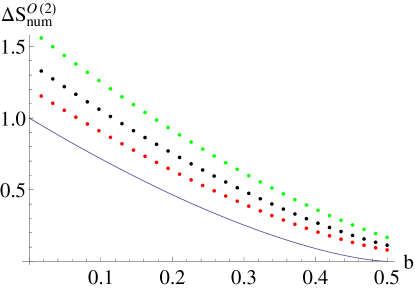
Figure 8: We take $\Delta Y=9$, $L_{s}=9$ and $\epsilon=1/100$. The red, black and green dots correspond to $D=0,1/3$ and $1/2$.

Finally, we briefly discuss effects adding the fundamental strings in $x^{8}$ direction. As we have done before, we find the Euclidean action after Legendre transformation to be

$$S_{E}=\int dt\left[2\pi LT_{DW}{1\over\Delta_{8}}\int dx^{8}{1\over R}\sqrt{(HR^{2}+B^{2})(1+\dot{R}^{2})(R^{2}+D^{2})}-\pi R^{2}L\Delta V\right].$$ (4.25)

Unfortunately in contrast to the previous cases, it is difficult to evaluate the bounce action even with fixed $x^{8}$. Thus, we have to require one more approximation and try to see the tendency of the gravitational correction to the bounce action. Suppose that $H$ is almost independent of $x^{8}$. This assumption limits the effective parameter region to be rather small. The harmonic function becomes

$$H_{0}\equiv 1+{L_{s}^{2}\over\Delta Y^{2}+q_{\rm meta}^{2}}.$$ (4.26)

By integrating over $x^{8}$, we obtain the simple expression

$$S_{E}=\int dt\left[2\pi LT_{DW}{1\over R}\sqrt{(H_{0}R^{2}+B^{2})(1+\dot{R}^{2})(R^{2}+D^{2})}-\pi R^{2}L\Delta V\right].$$ (4.27)

We use dimensionless variables

$$s={{\Delta V}\over 2\sqrt{H_{0}}T_{DW}}\tau,\quad r={{\Delta V}\over 2\sqrt{H_{0}}T_{DW}}R,\quad\tilde{b}={{\Delta V}\over 2H_{0}T_{DW}}B,\quad\tilde{d}={{\Delta V}\over 2\sqrt{H_{0}}T_{DW}}D.$$ (4.28)

Then,

$$S_{E} = \int ds{8\pi LT_{DW}^{3}\over{(\Delta V)^{2}}}H_{0}^{3/2}\left[{1\over r}\sqrt{(r^{2}+\tilde{b}^{2})(1+\dot{r}^{2})(r^{2}+\tilde{d}^{2})}-r^{2}\right]$$ (4.29)

$$= \int ds{8\pi LT_{DW}^{3}\over{(\Delta V)^{2}}}H_{0}^{3/2}\left[{1\over r}\sqrt{(r^{2}+{b^{2}\over{H_{0}^{2}}})(1+\dot{r}^{2})(r^{2}+{d^{2}\over{H_{0}}})}-r^{2}\right]$$

$$= {8\pi LT_{DW}^{3}\over{(\Delta V)^{2}}}S_{\rm num}^{O(2)}$$

$$= 3lB_{O(4)}S_{\rm num}^{O(2)},$$

where we have defined $l\equiv\left({2/3}\right)^{4}{\Delta VL/\pi T_{DW}}$. By defining the rescaled variables, $b/H_{0}$ and $d/\sqrt{H_{0}}$, the action becomes the same as the one in [6] up to overall factor $H^{3/2}_{0}$. Hence, we can easily evaluate the bounce action using the results in [6]. For the numerical estimation, it is useful to rewrite the bounce action formally as follows:

$$B_{O(2)}^{\rm grav} = {16\pi LT_{DW}^{3}\over{(\Delta V)^{2}}}\Delta S_{\rm num}^{O(2)}$$ (4.30)

$$= 6lB_{O(4)}\Delta S_{\rm num}^{O(2)}.$$

We plot $\Delta S_{\rm num}^{O(2)}$ as a function of $b$ in figure 9. Again we have found the tendency that the gravitational correction stabilizes the bubble, even with a string winding toward $x^{8}$ direction.

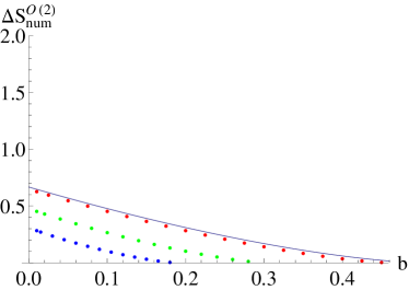
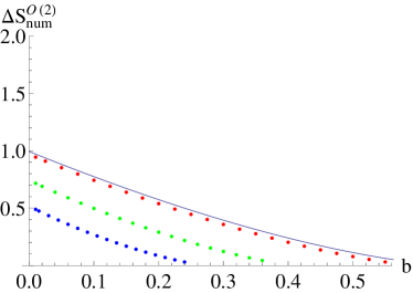
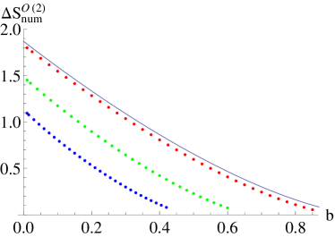
Figure 9: In each figure, the blue line corresponds to $d=0$. The red, green, and blue dots correspond to $d=1/100$, $d=1/10$, $d=2/10$ respectively. In the upper left panel, we take $\Delta Y=0,L_{s}=0$ (no gravity). In the upper right panel, we take $\Delta Y=9,L_{s}=5$. In the lower panel, we take $\Delta Y=9,L_{s}=9$.

5 Conclusions and discussions

In this paper, we have studied transitions between false and true vacua. These vacua were engineered by brane configurations in Type IIA string theory. We discussed the inhomogeneous vacuum decay via a $O(2)$ symmetric bubble induced by a cosmic string in the false vacuum. In the decay process, the bubble and the string formed a bound state which corresponds to the dielectric brane in the context of string theory. We found that the lifetime of the false vacuum becomes shorter in a wide range of parameter space. However, remarkably, when the induced magnetic field on the dielectric brane is smaller than the critical value, this catalysis does not work. This is in contrast to the results in the first paper [6]. We also discussed the leading order gravitational corrections in ten-dimension by treating the $NS_{3}$ brane as the background metric of the extremal black brane solution. This correction induced the force (basically) pulling the domain wall back to the origin in the internal space. And this force made the potential barrier higher and therefore the decay rate became smaller.

To proceed our studies further, it would be important to incorporate finite temperature effects. In the present brane setup, the finite temperature effects can be treated by using the non-extremal black brane solutions [34]. However, the analysis would become quite involved by the following two reasons. One is that since all $NS$-five branes are replaced by the black brane solutions, the original metastable configuration itself is distorted by the temperature effects. Therefore existence of the metastable state itself is not obvious in some parameter region. The other reason is that in a finite temperature system, the states are given by the Boltzmann distribution, so the initial point of the decay is not always the minimum of the potential. Thus we have to evaluate the thermally assisted decay rate and this analysis makes evaluation of the bounce action complicated. Also, to show generosity of inhomogenious decay in string landscape, it would be interesting to extend our studies of gravitational effects to geometrically induced metastable vacua [35, 36]. However, these studies are beyond the scope of this paper, so we would like to leave them future works.

References

- [1] R. Bousso and J. Polchinski, JHEP 0006, 006 (2000) [hep-th/0004134]: S. Kachru, R. Kallosh, A. D. Linde and S. P. Trivedi, Phys. Rev. D 68, 046005 (2003) [hep-th/0301240]: L. Susskind, In Carr, Bernard (ed.): Universe or multiverse? 247-266 [hep-th/0302219]: S. Ashok and M. R. Douglas, JHEP 0401, 060 (2004) [hep-th/0307049].
- [2] T. Banks, hep-th/0211160.
- [3] A. Aguirre and M. C. Johnson, Phys. Rev. D 77, 123536 (2008) [arXiv:0712.3038 [hep-th]]: A. Aguirre, T. Banks and M. Johnson, JHEP 0608, 065 (2006) [hep-th/0603107].
- [4] M. Dine, G. Festuccia and A. Morisse, JHEP 0909, 013 (2009) [arXiv:0901.1169 [hep-th]].
- [5] B. Greene, D. Kagan, A. Masoumi, D. Mehta, E. J. Weinberg and X. Xiao, Phys. Rev. D 88, no. 2, 026005 (2013) [arXiv:1303.4428 [hep-th]].
- [6] A. Kasai and Y. Ookouchi, arXiv:1502.01544 [hep-th].
- [7] R. C. Myers, JHEP 9912, 022 (1999) [hep-th/9910053].
- [8] R. Emparan, Phys. Lett. B 423, 71 (1998) [hep-th/9711106].
- [9] D. Mateos and P. K. Townsend, Phys. Rev. Lett. 87, 011602 (2001) [hep-th/0103030].
- [10] S. Kachru, J. Pearson and H. L. Verlinde, JHEP 0206, 021 (2002) [hep-th/0112197].
- [11] A. R. Frey, M. Lippert and B. Williams, Phys. Rev. D 68, 046008 (2003) [hep-th/0305018].
- [12] U. H. Danielsson and T. Van Riet, arXiv:1410.8476 [hep-th]: I. Bena, M. Grana, S. Kuperstein and S. Massai, arXiv:1410.7776 [hep-th]: U. H. Danielsson, arXiv:1502.01234 [hep-th].
- [13] P. J. Steinhardt, Nucl. Phys. B 190, 583 (1981); Phys. Rev. D 24, 842 (1981).
- [14] Y. Hosotani, Phys. Rev. D 27, 789 (1983).
- [15] U. A. Yajnik, Phys. Rev. D 34, 1237 (1986).
- [16] B. Kumar, M. B. Paranjape and U. A. Yajnik, Phys. Rev. D 82, 025022 (2010) [arXiv:1006.0693 [hep-th]]: B. Kumar and U. Yajnik, Nucl. Phys. B 831, 162 (2010) [arXiv:0908.3949 [hep-th]]: B. Kumar and U. A. Yajnik, Phys. Rev. D 79, 065001 (2009) [arXiv:0807.3254 [hep-th]].
- [17] T. Hiramatsu, M. Eto, K. Kamada, T. Kobayashi and Y. Ookouchi, JHEP 1401, 165 (2014) [arXiv:1304.0623 [hep-ph]]: K. Kamada, T. Kobayashi, K. Ohashi and Y. Ookouchi, JHEP 1305, 091 (2013) [arXiv:1303.2740 [hep-ph]]: M. Eto, Y. Hamada, K. Kamada, T. Kobayashi, K. Ohashi and Y. Ookouchi, JHEP 1303, 159 (2013) [arXiv:1211.7237 [hep-th]].
- [18] B. H. Lee, W. Lee, R. MacKenzie, M. B. Paranjape, U. A. Yajnik and D. h. Yeom, Phys. Rev. D 88, 085031 (2013) [arXiv:1308.3501 [hep-th]].
- [19] H. Ooguri and Y. Ookouchi, Phys. Lett. B 641, 323 (2006) [hep-th/0607183].
- [20] S. Franco, I. Garcia-Etxebarria and A. M. Uranga, JHEP 0701, 085 (2007) [hep-th/0607218].
- [21] I. Bena, E. Gorbatov, S. Hellerman, N. Seiberg and D. Shih, JHEP 0611, 088 (2006) [hep-th/0608157].
- [22] A. Giveon and D. Kutasov, Nucl. Phys. B 778, 129 (2007) [hep-th/0703135 [hep-th]]: Nucl. Phys. B 796, 25 (2008) [arXiv:0710.0894 [hep-th]].
- [23] M. Eto, K. Hashimoto and S. Terashima, JHEP 0703, 061 (2007) [hep-th/0610042].
- [24] R. Kitano, H. Ooguri and Y. Ookouchi, Ann. Rev. Nucl. Part. Sci. 60, 491 (2010) [arXiv:1001.4535 [hep-th]].
- [25] M. J. Duncan and L. G. Jensen, Phys. Lett. B 291, 109 (1992).
- [26] S. R. Coleman, Phys. Rev. D 15, 2929 (1977) [Erratum-ibid. D 16, 1248 (1977)].
- [27] K. A. Intriligator, N. Seiberg and D. Shih, JHEP 0604, 021 (2006) [hep-th/0602239].
- [28] A. Giveon, D. Kutasov, J. McOrist and A. B. Royston, Nucl. Phys. B 822, 106 (2009) [arXiv:0904.0459 [hep-th]].
- [29] G. T. Horowitz and A. Strominger, Nucl. Phys. B 360, 197 (1991).
- [30] K. Hashimoto, JHEP 0207, 035 (2002) [hep-th/0204203].
- [31] Y. Hyakutake, JHEP 0105, 013 (2001) [hep-th/0103146].
- [32] D. K. Park, S. Tamarian, Y. G. Miao and H. J. W. Muller-Kirsten, Nucl. Phys. B 606, 84 (2001) [hep-th/0011116]. D. K. Park, S. Tamarian and H. J. W. Muller-Kirsten, JHEP 0205, 009 (2002) [hep-th/0012108].
- [33] J. Polchinski, Cambridge University Press (1998): B. Zwiebach, Cambridge University Press (2009).
- [34] D. Kutasov, O. Lunin, J. McOrist and A. B. Royston, Nucl. Phys. B 833, 64 (2010) [arXiv:0909.3319 [hep-th]].
- [35] H. Ooguri and Y. Ookouchi, Nucl. Phys. B 755, 239 (2006) [hep-th/0606061]: M. Aganagic, C. Beem, J. Seo and C. Vafa, Nucl. Phys. B 789, 382 (2008) [hep-th/0610249]: R. Kitano, H. Ooguri and Y. Ookouchi, Phys. Rev. D 75, 045022 (2007) [hep-ph/0612139]: R. Argurio, M. Bertolini, S. Franco and S. Kachru, JHEP 0706, 017 (2007) [AIP Conf. Proc. 1031, 94 (2008)] [hep-th/0703236].
- [36] H. Ooguri, Y. Ookouchi and C. S. Park, Adv. Theor. Math. Phys. 12, 405 (2008) [arXiv:0704.3613 [hep-th]]: R. Auzzi and E. Rabinovici, JHEP 1008, 044 (2010) [arXiv:1006.0637 [hep-th]]: J. Marsano, H. Ooguri, Y. Ookouchi and C. S. Park, Nucl. Phys. B 798, 17 (2008) [arXiv:0712.3305 [hep-th]]: G. Pastras, JHEP 1310, 060 (2013) [arXiv:0705.0505 [hep-th]].