Some aspects of symmetric Gamma process mixtures

Abstract.

In this article, we present some specific aspects of symmetric Gamma process mixtures for use in regression models. We propose a new Gibbs sampler for simulating the posterior and we establish adaptive posterior rates of convergence related to the Gaussian mean regression problem.

1. Introduction

Recently, interest in a Bayesian nonparametric approach to the sparse regression problem based on mixtures emerged from works of Abramovich et al. (2000), de Jonge and van Zanten (2010) and Wolpert et al. (2011). The idea is to model the regression function as

$$f(\cdot)=\int_{\mathcal{X}}K(x;\cdot)Q(dx),\quad Q\sim\Pi_{*},$$ (1)

where $K:\mathcal{X}\times\operatorname{\mathbb{R}}^{d}\rightarrow\operatorname{\mathbb{R}}$ is a jointly measurable kernel function, and $\Pi_{*}$ a prior distribution on the space of signed measure over the measurable space $\mathcal{X}$. Although the model (1) is popular in density estimation Escobar and West (1994); Müller et al. (1996); Ghosal and van der Vaart (2007a); Shen et al. (2013); Canale and De Blasi (2013) and for modeling hazard rates in Bayesian nonparametric survival analysis Lo and Weng (1989); Peccati and Prünster (2008); De Blasi et al. (2009); Ishwaran and James (2012); Lijoi and Nipoti (2014), it seems that much less interest has been shown in regression.

Perhaps the little interest for mixture models in regression is due to the lack of variety in the choice of algorithms available, and in the insufficiency of theoretical posterior contraction results. To our knowledge, the sole algorithm existing for posterior simulations is to be found in Wolpert et al. (2011), when the mixing measure $Q$ is a Lévy process. On the other hand, The only contraction result available is to be found in de Jonge and van Zanten (2010) for a suitable semiparametric mixing measure.

Indeed, both designing an algorithm or establishing posterior contraction results heavily depends on the choice of $K$ and $\Pi_{*}$ in equation 1; but above all also on the observation model we consider. This last point makes the study of mixtures in regression nasty to handle because of the diversity of observation models possible. In this article, we focus on the situation when $Q$ is a symmetric Gamma process to propose both a new algorithm for posterior simulations and posterior contraction rates results.

In the first part of the paper, we propose a Gibbs sampler to get samples from the posterior distribution of symmetric Gamma process mixtures. The algorithm is sufficiently general to be used in all observation models for which the likelihood function is available. We begin with some preliminary theoretical result about approximating symmetric Gamma process mixtures, before stating the general algorithm. Finally, we make an empirical study of the algorithm, with comparison with the RJMCMC algorithm of Wolpert et al. (2011).

The second part of the paper is devoted to posterior contraction rates results. We consider the mean regression model with normal errors of unknown variance, and two types of mixture priors: location-scale and location-modulation. The latter has never been studied previously, mainly because it is irrelevant in density estimation models. However, we show here that it allows to get better rates of convergence than location-scale mixtures, and thus might be interesting to consider in regression.

2. Symmetric Gamma process mixtures

Let $(\Omega,\mathcal{E},\mathbb{P})$ be a probability space and $(\mathcal{X},\mathcal{A})$ be a measurable space. We call a mapping $Q:\Omega\times\mathcal{A}\rightarrow\operatorname{\mathbb{R}}\cup\{\pm\infty\}$ a signed random measure if $\omega\mapsto Q(\omega,A)$ is a random variable for each $A\in\mathcal{A}$ and if $A\mapsto Q(\omega,A)$ is a signed measure for each $\omega\in\Omega$.

Symmetric Gamma random measures are infinitely divisible and independently scattered random measures (the terminology Lévy base is also used in Barndorff-Nielsen and Schmiegel (2004), and Lévy random measure in Wolpert et al. (2011)), that is, random measures with the property that for each disjoint $A_{1},\dots,A_{k}\in\mathcal{A}$, the random variables $Q(A_{1}),\dots,Q(A_{k})$ are independent with infinitely divisible distribution. More precisely, given $\alpha,\eta>0$ and $F$ a probability measure on $\mathcal{X}$, a symmetric Gamma random measure assigns to all measurable set $A\in\mathcal{A}$ random variables with distribution $\mathrm{SGa}(\alpha F(A),\eta)$ (see appendix A). Existence and uniqueness of symmetric Gamma random measures is stated in Rajput and Rosinski (1989).

In the sequel, we shall always denote by $\Pi_{*}$ the distribution of a symmetric Gamma random measure with parameters $\alpha,\eta$ and $F$, and we refer $\alpha F$ as the base distribution of $Q\sim\Pi_{*}$, and $\eta$ as the scale parameter.

2.1. Location-scale mixtures

Given a measurable mother function $g:\operatorname{\mathbb{R}}^{d}\rightarrow\operatorname{\mathbb{R}}$, we define the location-scale kernel $K_{A}(x):=g(A^{-1}x)$, for all $x\in\operatorname{\mathbb{R}}^{d}$ and all $A\in\mathcal{E}$, where $\mathcal{E}$ denote the set of all $d\times d$ positive definite real matrices. Then we consider symmetric Gamma location-scale mixtures of the type

$$f(x;\omega):=\int_{\mathcal{E}\times\operatorname{\mathbb{R}}^{d}}K_{A}(x-\mu)\,Q(dAd\mu;\omega),\qquad\forall x\in\operatorname{\mathbb{R}}^{d},$$ (2)

where $Q:\mathcal{E}\times\operatorname{\mathbb{R}}^{d}\times\Omega\rightarrow[-\infty,\infty]$ is a symmetric Gamma random measure with base measure $\alpha F$ on $\mathcal{E}\times\operatorname{\mathbb{R}}^{d}$, and scale parameter $\eta>0$. The precise meaning of the integral in equation 2 is made clear in Rajput and Rosinski (1989).

2.2. Location-modulation mixtures

As in the previous section, given a measurable mother function $g:\operatorname{\mathbb{R}}^{d}\rightarrow\operatorname{\mathbb{R}}$, we define the location-modulation kernel $K_{\xi,\phi}(x):=g(x)\cos(\sum_{i=1}^{d}\xi x_{i}+\phi)$, for all $x\in\operatorname{\mathbb{R}}^{d}$, all $\xi\in\operatorname{\mathbb{R}}^{d}$ and all $\phi\in[0,\pi/2]$. Then we consider symmetric Gamma location-modulation mixtures of the type

$$f(x;\omega):=\int_{\operatorname{\mathbb{R}}^{d}\times\operatorname{\mathbb{R}}^{d}\times[0,\pi/2]}K_{\xi,\phi}(x-\mu)\,Q(d\xi d\mu d\phi;\omega),\qquad\forall x\in\operatorname{\mathbb{R}}^{d},$$ (3)

where $Q:\operatorname{\mathbb{R}}^{d}\times\operatorname{\mathbb{R}}^{d}\times[0,\pi/2]\times\Omega\rightarrow[-\infty,\infty]$ is a symmetric Gamma random measure with base measure $\alpha F$ on $\operatorname{\mathbb{R}}^{d}\times\operatorname{\mathbb{R}}^{d}\times[0,\pi/2]$, and scale parameter $\eta>0$.

2.3. Convergence of mixtures

Given a kernel $K:\mathcal{X}\times\operatorname{\mathbb{R}}^{d}\rightarrow\operatorname{\mathbb{R}}$ and a symmetric Gamma random measure $Q$, it is not clear a priori whether or not the mixture $y\mapsto\int K(x;y)\,Q(dx)$ converges or not, and in what sense. According to Rajput and Rosinski (1989) (see also Wolpert et al. (2011)), $y\mapsto\int K(x;y)\,Q(dx)$ converges almost-surely at all $y$ for which

$$\int_{\operatorname{\mathbb{R}}\times\mathcal{X}}(1\wedge|uK(x;y)|)|u|^{-1}e^{-|u|\eta}F(dx)<+\infty.$$

Moreover, from the same references (or also in Kingman (1992)), if $M$ is a complete normed space equipped with norm $\|\cdot\|$, then $y\mapsto\int K(x;y)\,Q(dx)$ converges almost-surely in $M$ if

$$\int_{\operatorname{\mathbb{R}}\times\mathcal{X}}(1\wedge|u|\|K(x;\cdot)\|)|u|^{-1}e^{-|u|\eta}F(dx)<+\infty.$$

Since by definition $F$ is a probability measure, we have for instance that the mixtures of equations 2 and 3 converges almost surely in $L^{\infty}$ as soon as $\|K_{A}\|_{\infty}<+\infty$ for $F$-almost every $A\in\mathcal{E}$, or $\|K_{\xi,\phi}\|_{\infty}<+\infty$ for $F$-almost every $(\xi,\phi)\in\operatorname{\mathbb{R}}^{d}\times[0,\pi/2]$.

3. Simulating the posterior

In this section we propose a Gibbs sampler for exploration of the posterior distribution of a mixture of kernels by a symmetric Gamma random measure. The sampler is based on the series representation of the next theorem, inspired from a result about Dirichlet processes from Favaro et al. (2012), adapted to symmetric Gamma processes. In theorem 1, we consider $\mathcal{M}(\mathcal{X})$ the space of signed Radon measures on the measurable space $(\mathcal{X},\mathcal{A})$. By the Riesz-Markov representation theorem (Rudin, 1974, Chapter 6), $\mathcal{M}(\mathcal{X})$ can be identified as the dual space of $\mathtt{C}_{c}(\mathcal{X})$, the space continuous functions with compact support. That said, we endow $\mathcal{M}(\mathcal{X})$ with the topology $\mathcal{T}_{v}$ of weak-* convergence (sometimes referred as the topology of vague convergence), that is, a sequence $\{\mu_{n}\in\mathcal{M}(\mathcal{X})\nonscript\,:\nonscript\,\mathopen{}\allowbreak n\in\operatorname{\mathbb{N}}\}$ converges to $\mu\in\mathcal{M}(\mathcal{X})$ with respect to the topology $\mathcal{T}_{v}$, if for all $f\in\mathtt{C}_{c}(\mathcal{X})$,

$$\int_{\mathcal{X}}f(x)\,d\mu_{n}(x)\rightarrow\int_{\mathcal{X}}f(x)\,d\mu(x).$$

Dealing with prior distributions on $\mathcal{M}(\mathcal{X})$, we shall equip $\mathcal{M}(\mathcal{X})$ with a $\sigma$-algebra. Here it is always considered the Borel $\sigma$-algebra of $\mathcal{M}(\mathcal{X})$ generated by $\mathcal{T}_{v}$.

Before stating the main theorem of this section, we recall that a sequence of random variables $\{X_{i}\in\mathcal{X}\nonscript\,:\nonscript\,\mathopen{}\allowbreak 1\leq i\leq n\}$ is a Pólya urn sequence with base distribution $\alpha F(\cdot)$, where $F$ is a probability distribution on $(\mathcal{X},\mathcal{A})$ and $\alpha>0$, if for all measurable set $A\in\mathcal{A}$,

$$P(X_{1}\in A)=F(A),\quad P(X_{k+1}\in A\,|\,X_{1},\dots,X_{k})=F_{k}(A)/F_{k}(\mathcal{X}),\ k=2,\dots,n-1,$$

where $F_{k}:=\alpha F+\sum_{i=1}^{k}\delta_{X_{i}}$. We are now in position to state the main theorem of this section, which proof is given in appendix A.

Theorem 1.

Let $\mathcal{X}$ be a Polish space with Borel $\sigma$-algebra, $p>0$ be integer, $T\sim\mathrm{Ga}(\alpha,\eta)$, independently, $J_{1},\dots,J_{p}\operatorname{\overset{\mathrm{i.i.d}}{\sim}}\mathrm{SGa}(1,1)$, and $\{X_{i}\in\mathcal{X}\nonscript\,:\nonscript\,\mathopen{}\allowbreak 1\leq i\leq p\}$ a Pólya urn sequence with base distribution $\alpha F(\cdot)$, independent of $T$ and of the $J_{i}$’s. Define the random measure, $Q_{p}:=\sqrt{T/p}\sum_{i=1}^{p}J_{i}\,\delta_{X_{i}}$. Then $Q_{p}\overset{d}{\rightarrow}Q$, where $Q$ is a symmetric Gamma random measure with base distribution $\alpha F(\cdot)$ and scale parameter $\sqrt{\eta}$.

3.1. Convergence of sequences of mixtures

In theorem 1, we proved weak convergence of the sequence of approximating measures $(Q_{p})_{p\geq 1}$ to the symmetric Gamma random measure, but it is not clear that mixtures of kernels by $Q_{p}$ also converge. The next proposition establish convergence in $L^{q}$ for general kernels, with $1\leq q<+\infty$, the proof is similar to the proof of Favaro et al. (2012, Theorem 2), thus we defer it into section 6.2. For any kernel $K:\mathcal{X}\times\operatorname{\mathbb{R}}^{d}\rightarrow\operatorname{\mathbb{C}}$, and any (signed) measure $Q$ on $(\mathcal{X},\mathcal{A})$, we write

$$f^{(Q)}(y):=\int_{\mathcal{X}}K(x;y)\,Q(dx).$$

Proposition 1.

If $x\mapsto K(x;y)$ is continuous for all $x\in\mathcal{X}$, vanishes outside a compact set, and bounded by a Lebesgue integrable function $h$, then for any $1\leq q<+\infty$ we have $\lim_{p\rightarrow\infty}\|f^{(Q_{p})}-f^{(Q)}\|_{q}=0$ almost-surely.

Under supplementary assumptions on $K$, we can say a little-more about uniform convergence of the approximating sequence of mixtures. Assuming that $y\mapsto K(x;y)$ is in $L^{1}$ for all $x\in\mathcal{X}$, we denote by $(x,u)\mapsto\widehat{K}(x;u)$ the $L^{1}$ Fourier transform on the second argument of $(x,y)\mapsto K(x;y)$.

Proposition 2.

Let $y\mapsto K(x;y)$ be in $L^{1}$ for all $x\in\mathcal{X}$ and $\widehat{K}$ satisfies the assumption of proposition 1. Then $\lim_{p\rightarrow\infty}\|f^{(Q_{p})}-f^{(Q)}\|_{\infty}=0$ almost-surely.

Proof.

We can assume without loss of generality that $f^{(Q_{p})}$ and $f^{(Q)}$ are defined on the same probability space $(\Omega,\mathcal{F},\mathbb{P})$. By duality, it is clear that $\|f^{(Q_{p})}(\cdot;\omega)-f^{(Q)}(\cdot;\omega)\|_{\infty}\leq\int_{\operatorname{\mathbb{R}}^{d}}|\widehat{f}^{(Q_{p})}(u,\omega)-\widehat{f}^{(Q)}(u;\omega)|\,du$, where $\widehat{f}$ denote the $L^{1}$ Fourier transform of $f$. Notice that by assumptions on $K$, $\widehat{f}^{(Q_{p})}$ and $\widehat{f}^{(Q)}$ are well-defined for almost all $\omega\in\Omega$ (see section 2.3). Then by Fubini’s theorem

$$\widehat{f}^{(Q_{p)}}(u;\omega) =\int_{\operatorname{\mathbb{R}}^{d}}\int_{\mathcal{X}}K(x;y)\,Q(dx;\omega)\,\operatorname{e}^{-iuy}\,dy$$

$$=\int_{\mathcal{X}}\int_{\operatorname{\mathbb{R}}^{d}}K(x;y)\operatorname{e}^{-iuy}\,dy\,Q(dx;\omega)=\int_{\mathcal{X}}\widehat{K}(x;u)\,Q(dx;\omega),$$

and the conclusion follows from proposition 1. ∎

3.2. General algorithm

From theorem 1, replacing $Q$ by $Q_{p}$ for sufficiently large $p$, we propose a Pólya urn Gibbs sampler adapted from algorithm 8 in Neal (2000). In the sequel, we refer to $Q_{p}$ as the particle approximation of $Q$ with $p$ particles.

Let $Y=(Y_{i})_{i=1}^{n}$ be observations coming from a statistical model with likelihood function $\mathcal{L}(f|Y)$, where $f:\operatorname{\mathbb{R}}^{d}\rightarrow\operatorname{\mathbb{R}}$ is the regression function on which we put a symmetric Gamma mixture prior distribution. Let $X=(X_{i})_{i=1}^{p}$ be a Pólya urn sequence, $J:=(J_{1},\dots,J_{p})$ a sequence of i.i.d. $\mathrm{SGa}(1,1)$ random variables, and $T\sim\operatorname{Ga}(\alpha,\eta)$ independent of $(X_{i})_{i=1}^{p}$ and $J$. We introduce the clustering variables $C:=(C_{1},\ldots,C_{p})$ such that $C_{i}=k$ if and only if $X_{i}=X_{k}^{\star}$ where $X^{\star}:=X_{1}^{\star},\ldots$ stands for unique values of $(X_{i})_{i=1}^{p}$. In the sequel, $C_{-i}$ stands for the vector obtained from removing the coordinate $i$ to $C$, and the same definition holds for $J$ mutatis mutandis. Given $J,C,X,T$ and a measurable kernel $K:\mathcal{X}\times\operatorname{\mathbb{R}}\rightarrow\operatorname{\mathbb{R}}$ we construct $f$ as

$$f(x)=\sqrt{\frac{T}{p}}\sum_{i=1}^{p}J_{i}\,K(X_{i};x).$$

We propose the following algorithm. At each iteration, successively sample from :

1. $C_{i}|C_{-i},Y,X,J,T$, for $1\leq i\leq p$. Let $n_{k,i}=\#_{\stackrel{{\scriptstyle 1\leq l\leq n}}{{l\neq i}}}\{C_{l}=k\}$, $\kappa^{(p)}$ the number of distinct $X_{k}$ values and $\kappa_{0}$ a chosen natural,

   $$C_{i} \stackrel{{\scriptstyle\text{ind}}}{{\sim}}\sum_{k=1}^{\kappa^{(p)}}n_{k,i}\,\mathcal{L}_{k,i}(X,J,T|Y)\,\delta_{k}(\cdot)+\frac{\alpha}{\kappa_{0}}\sum_{k=1}^{\kappa_{0}}\mathcal{L}_{k+\kappa^{(p)},i}(X,J,T|Y)\,\delta_{k+\kappa^{(p)}}(\cdot),$$

   where $\mathcal{L}_{k,i}(X,J,T|Y)$ stands for the likelihood under hypothesis that particle $i$ is allocated to component $k$ (note that the likelihood evaluation requires the knowledge of whole distribution $F$ under any allocation hypothesis).

2. $X|C,Y,J,T$. Random Walk Metropolis Hastings on parameters.

3. $J_{i}|J_{-i},K,Y,X,T$, for $1\leq i\leq p$. Independent Metropolis Hastings with prior $\mathrm{SGa}(1,1)$ taken as i.i.d. candidate distribution for $J_{i}$. Note that for $n\rightarrow\infty$, the posterior distribution of $J_{i}|J_{-i},C,Y,Z$ should be $\mathrm{SGa}(1,1)$, then the number of particles $p$ may be monitored using the acceptance ratio of the $J_{i}$’s.

4. $T|C,Y,X,J$. Random Walk Metropolis Hastings on scale parameter.

3.3. Assessing the convergence of the Markov Chain

The previous algorithm produces a Markov Chain whose invariant distribution is (an approximation of) the posterior distribution of a symmetric Gamma process mixture. However, if the Markov Chain is initialized in a region of low posterior probability mass, we may over-sample this region. To avoid such over-sampling, we discard the first $n_{0}$ samples of the chain using Geweke’s convergence diagnostic (Geweke, 1992).

More precisely, we monitor the convergence of the chain using the log-likelihood function. We start the algorithm with Markov Chain initialized at random from prior distribution. Then after $n\gg n_{0}$ iterations we compute Geweke’s $Z$-statistic for the log-likelihood using the whole chain; if the statistic is outside the $95\%$ confidence interval we continue to apply the diagnostic after discarding $10\%$, $20\%$, $30\%$ and $40\%$ of the chain. If the $Z$-statistic is still outside $95\%$ confidence interval, the chain is reported as failed to converge, and we restart the algorithm from a different initialization point.

Once we have discarded the first $n_{0}$ samples using Geweke’s test, we run the chain sufficiently longer to get an Effective Sample Size (ESS) of at least $1000$ samples, where we measure the ESS through the value of the log-likelihood at each iteration of the Markov Chain. A thinning of the chain is not required in general, however, we found in practice that a slight thinning improves the efficiency of the sampling.

In fig. 1, we draw some examples of temporal evolution of the log-likelihood on a simple univariate Gaussian mean regression problem. Here and after, we always choose step sizes in RWMH steps to achieve approximately 30% acceptance rates for each class of updates. Each subfigure represent 10 simulations with random starting point of the Markov Chain, distributed according to the prior distribution. We draw each subfigure varying the parameters liable to influence the mixing time of the chain, notably $m$ and the number of particles. We observe that the speed at which the chain reach equilibrium is fast, especially when the number of particles is high. This last remark have to be balanced with the complexity in time of the algorithm which is $O(mnp)$ for a naive implementation, and, depending on the nature of the likelihood, can be reduced to $O(mp)$ or $O(mp^{2})$.

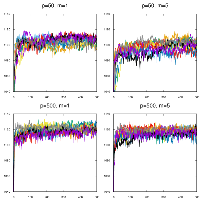
Figure 1. Time evolution of the log-likelihood for different starting point of the Markov Chain, chosen according to the prior distribution, and various parameters of the algorithm. The figure are taken from the test function blip of the section 4.1.

4. Examples of simulations

We now turn our attention to simulated examples to illustrate the performance of mixture models. First, we use mixtures as a prior distribution on the regression function in the univariate mean regression problem with normal errors. Of course, the interest for mixture comes when the statistical model is more involved. Hence, in a second time we present simulation results for the multivariate inverse problem of CT imaging.

4.1. Mean regression with normal errors

We present results of our algorithm on several standard test functions from the wavelet regression litterature (see Marron et al., 1998), following the methodology from Antoniadis et al. (2001) (i.e. Gaussian mean regression with fixed design and unknown variance). However, it should be noticed that mixtures are not a Bayesian new implementation of wavelet regression, and are much more general (see for instance the next section). For each test function, the noise variance is chosen so that the root signal-to-noise ratio is equal to 3 (a high noise level) and a simulation run was repeated 100 times with all simulation parameters constant, excepting the noise which was regenerated. We ran the algorithm for location-scale mixtures of Gaussians and Symmlet8, with normal $\mathrm{N}(0.5,0.3)$ distribution as prior distribution on translations, and a mixture of Gamma distributions for scales ($\mathrm{Ga}(30,0.06)$ and $\mathrm{Ga}(2,0.04)$ with expectation $500$ and $50$ respectively). In addition of the core algorithm of section 3.2, we also added

• a Gibbs step estimation of the noise variance, with Inverse-Gamma prior distributon,

• a $\mathrm{Ga}(2,0.5)$ (with expectation $4$) prior on $\alpha$, with sampling of $\alpha$ done through a Gibbs update according to the method proposed in West (1992),

• a Dirichlet prior on the weights of the mixture of $\mathrm{Ga}(20,0.2)$ and $\mathrm{Ga}(2,0.1)$, with sampling of the mixture weights done through Gibbs sampling in a standard way,

• a $\mathrm{Ga}(5,10)$ (with expectation $0.5)$ prior on $T$, instead of normally $\mathrm{Ga(\alpha,\eta})$, which add more flexibility.

The choice of the mixture distribution as prior on scales may appear surprising, but we found in practice that using bimodal distribution on scales substantially improve performance of the algorithm, especially when there are few data available and/or high noise, because in general both large and small scales components are needed to estimate the regression function.

We ran the algorithm for $n=128$ and $n=1024$ data, and the performance is measured by its average root mean square error, defined as the average of the square root of the mean squared error $n^{-1}\sum_{i=1}^{n}|\widehat{f}(x_{i})-f_{0}(x_{i})|^{2}$, with $\widehat{f}$ denoting the posterior mean and $f_{0}$ the true function. We ran on the same dataset the Translation-Invariant with hard thresholding algorithm (TI-H) and Symmlet8 wavelets (see Antoniadis et al. (2001)), which is one of the best performing algorithm on this collection of test functions. We ran our algorithm with Symmlet8 kernels to make this comparison more relevant, since the choice of the kernel has major impact on the performance of the algorithm (see section 4.1.4 below).

4.1.1. Alternatives

In Wolpert et al. (2011), authors develop a reversible-jump MCMC scheme where the random measure is thresholded, i.e. small jumps are removed, yielding to a compound Poisson process approximation of the random measure, with almost-surely a finite number of jumps, allowing numerical computations. We also ran their algorithm with a thresholding level of $\epsilon=0.05$ (which seems to give the best performance), a $\mathrm{Ga}(15,1)$ prior on $\eta$, and all other parameters being exactly the same as described in the previous section. We use the criteria of section 3.3 to stop the running of the chain.

4.1.2. Choosing the number of particles

It is not clear how to choose the number of particles in the algorithm. In theory, the higher is the better. In practice, however, we recommend choosing the number of particles according to the acceptance rate of particles weights move in step 3 of the algorithm. We found in practice that a level of acceptance between 20% and 30% is acceptable, as illustrated in fig. 2.

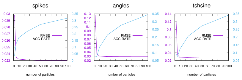
Figure 2. Mean over 100 runs of RMSE versus acceptance rate in step 3 of the algorithm for some typical test functions. For each signal the number of covariates is set to 128 and the RNSR is equal to 3.

4.1.3. Simulation results

In tables 1 and 2 we summarize the results for location-scale mixtures of Gaussians and Symmlet8 produced by the algorithm of section 3.2 and by the RJMCMC algorithm of Wolpert et al. (2011), with the TI-H method as reference. We used $p=150$ particles for both the datasets with $n=128$ covariates and $n=1024$ covariates, which is a nice compromise in terms of performance and computational cost. Regarding our algorithm and the RJMCMC algorithm, no particular effort was made to determine the value of the fixed parameters.

	TI-H	Gibbs		RJMCMC
Function	Symm8	Gauss	Symm8	Gauss	Symm8
step	0.0589	0.0517	0.0551	0.0550	0.0565
wave	0.0319	0.0323	0.0306	0.0342	0.0370
blip	0.0307	0.0301	0.0316	0.0323	0.0373
blocks	0.0464	0.0343	0.0374	0.0383	0.0418
bumps	0.0285	0.0162	0.0229	0.0224	0.0345
heavisine	0.0257	0.0267	0.0264	0.0280	0.0289
doppler	0.0443	0.0506	0.0418	0.0526	0.0493
angles	0.0293	0.0266	0.0282	0.0274	0.0305
parabolas	0.0344	0.0301	0.0307	0.0312	0.0396
tshsine	0.0255	0.0285	0.0277	0.0291	0.0339
spikes	0.0237	0.0178	0.0207	0.0199	0.0218
corner	0.0177	0.0171	0.0170	0.0182	0.0255

Table 1. Summary of root mean squared errors of different algorithms for $n=128$ covariates and a root signal to noise ratio of $3$.

	TI-H	Gibbs		RJMCMC
Function	Symm8	Gauss	Symm8	Gauss	Symm8
step	0.0276	0.0268	0.0289	0.0282	0.0300
wave	0.0088	0.0118	0.0108	0.0133	0.0117
blip	0.0148	0.0162	0.0172	0.0180	0.0183
blocks	0.0222	0.0230	0.0241	0.0247	0.0256
bumps	0.0122	0.0132	0.0182	0.0201	0.0232
heavisine	0.0154	0.0134	0.0139	0.0147	0.0147
doppler	0.0180	0.0207	0.0196	0.0261	0.0225
angles	0.0123	0.0120	0.0123	0.0125	0.0128
parabolas	0.0135	0.0124	0.0132	0.0147	0.0145
tshsine	0.0107	0.0109	0.0111	0.0131	0.0120
spikes	0.0110	0.0075	0.0095	0.0095	0.0103
corner	0.0077	0.0075	0.0081	0.0095	0.0085

Table 2. Summary of root mean squared errors of different algorithms for $n=1024$ covariates and a root signal to noise ratio of $3$.

Obviously the Gibbs algorithm allow for sampling the full posterior distribution, pemitting estimation of posterior credible bands, as illustrated in figs. 3 and 4, where the credible bands were drawn retaining the $95\%$ samples with the smaller $\ell_{2}$-distance with respect to the posterior mean estimator. Although the algorithm samples an approximated version of the model, it is found that the accuracy of credible bands is quite good since the true regression function almost never comes outside the sampled $95\%$ bands, as it is visible in the example of figs. 3 and 4. Despite the algorithm efficiency, future work should be done to develop new sampling techniques for regression with mixture models, mainly to improve computation cost.

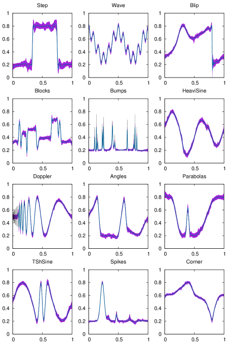
Figure 3. Example of simulation results using location-scale mixtures of Gaussians. The root signal-to-noise ratio is equal to 3 for sample size of 1024 design points. The true regression function is represented with dashes, the mean of the sampled posterior distribution in blue and sampled 95% credible bands in pink.

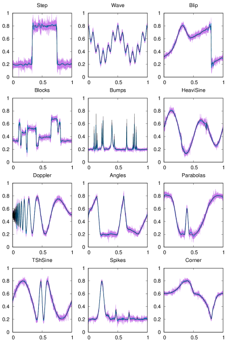
Figure 4. Example of simulation results using location-scale mixtures of Symmlet8. The root signal-to-noise ratio is equal to 3 for sample size of 1024 design points. The true regression function is represented with dashes, the mean of the sampled posterior distribution in blue and sampled 95% credible bands in pink.

4.1.4. Discussion

Obviously, the computation cost for our algorithm is high compared to TI-H, or any other classical wavelet thresholding method, even considering that it can intrinsically compute credible bands. But, as mentioned in Antoniadis et al. (2001), the choice of the kernel is crucial to the performance of estimators. The attractiveness of mixtures then comes because we are not restricted to location-scale or location-modulation kernels, and almost any function is acceptable as a kernel, which is not the case for most regression methods. Moreover, there is no requirements on how the data are spread, which makes the method interesting in inverse problems, such as in the next section.

4.2. Multivariate inverse problem example

Many medical imaging modalities, such as X-ray computed tomography imaging (CT), can be described mathematically as collecting data in a Radon transform domain. The process of inverting the Radon transform to form an image can be unstable when the data collected contain noise, so that the inversion needs to be regularized in some way. Here we model the image of interest as a measurable function $f:\mathbb{R}^{2}\rightarrow\mathbb{R}$, and we propose to use a location-scale mixtures of Gaussians to regularize the inversion of the Radon transform.

More precisely, the Radon transform $R_{f}:\mathbb{R}^{+}\times[0,\pi]\rightarrow\mathbb{R}$ of $f$ is such that $R_{f}(r,\theta)=\int_{-\infty}^{+\infty}f(r\cos\theta-t\sin\theta,r\sin\theta+\cos\theta)\,dt$. Then we consider the following model. Let $n,m\geq 1$. Assuming that the image is supported on $[-1,1]^{2}$ we let $r_{1},\dots,r_{n}$ equidistributed in $[-\sqrt{2},\sqrt{2}]$ and $\theta_{1},\dots,\theta_{m}$ equidistributed in $[0,\pi]$. Then,

$$Y_{nm}\sim\mathrm{N}(R_{f}(x_{n},\theta_{m}),\sigma^{2})\quad\forall n,m$$

$$f\sim\Pi,$$

where $\Pi$ is a symmetric Gamma process location-scale mixture with base measure $\alpha F_{A}\times F_{\mu}$ on $\mathcal{E}\times\mathbb{R}^{2}$, $\alpha>0$, and scale parameter $\eta>0$. In the sequel, we use a normal distribution with mean zero and covariance matrix $\mathrm{diag}(\tau,\tau)$ as distribution for $F_{\mu}$. Regarding $F_{A}$, the choice is more delicate; we choose a prior distribution over the set of shearlet-type matrices of the form

$$\begin{pmatrix}1&s\\ 0&1\end{pmatrix}\begin{pmatrix}a&0\\ 0&\sqrt{a}\end{pmatrix},$$

where we set a $\mathrm{N}(1,\sigma_{a}^{2})$ distribution over the coefficient $a$ and $\mathrm{N}(0,\sigma_{s}^{2})$ over the coefficient $s$. This type of prior distribution for $F_{A}$ is particularly convenient for capturing anisotropic features such as edges in images (Easley et al., 2009).

We ran our algorithm for $n=256$ and $m=128$ ($32768$ observations, a small amount), using the Shepp and Logan phantom as original image (Shepp and Logan, 1974). The variance of the noise is $\sigma^{2}=0.1$, whereas the image take value between $0$ and $2$. Both the original image and the reconstruction are visible in fig. 5. Finally, we should mention that the choice of the Gaussian kernel for the mixture is convenient since it allows to compute the likelihood analytically. However, from a practical side, a full implementation of the algorithm with the intention of reconstructing CT images may benefit from using a different kernel.

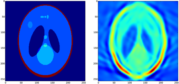
Figure 5. Simulation of X-ray computed tomography imaging using symmetric Gamma process location-scale mixture of Gaussians. On the left: the original image. On the right: the reconstructed image from $32768$ observations of the Radon transform of the original image in a Gaussian noise.

5. Rates of convergence

In this section, we investigate posterior convergence rates in fixed design Gaussian regression for both symmetric Gamma location-scale mixtures and symmetric Gamma location-modulation mixtures.

5.1. Notations

In the sequel we use repeatedly the following notations.

• The conventional multi-index notation, for all $\alpha=(\alpha_{1},\dots,\alpha_{d})\in\operatorname{\mathbb{N}}^{d}$ and all $z=(z_{1},\dots,z_{d})\in\operatorname{\mathbb{R}}^{d}$ we write $|\alpha|:=\alpha_{1}+\dots+\alpha_{d}$, $\alpha!:=\alpha_{1}!\dots\alpha_{d}!$, and $z^{\alpha}:=z_{1}^{\alpha_{1}}\dots z_{d}^{\alpha_{d}}$. Moreover, for all $f:\operatorname{\mathbb{R}}^{d}\rightarrow\operatorname{\mathbb{R}}$ with continuous $k$-th order partial derivatives at $x\in\operatorname{\mathbb{R}}^{d}$ we write

  $$D^{\alpha}f(x):=\frac{\partial^{|\alpha|}f}{\partial z_{1}^{\alpha_{1}}\dots\partial z_{n}^{\alpha_{d}}}(x),\quad|\alpha|\leq k.$$

• Let $\Omega$ be an open subset of $\operatorname{\mathbb{R}}^{d}$ and $\overline{\Omega}$ be the closure of $\Omega$. For any $\beta>0$, we define $\mathcal{C}^{\beta}(\overline{\Omega})$, the Hölder space on $\overline{\Omega}$, as the set of all functions on $\overline{\Omega}$ such that $\|f\|_{\mathcal{C}^{\beta}}:=\max_{|\alpha|\leq k}\sup_{x\in\Omega}|D^{\alpha}f(x)|+\max_{|\alpha|=k}\sup_{x\neq y\in\Omega}|D^{\alpha}f(x)-D^{\alpha}f(y)|/|x-y|^{\beta-k}$ is finite, where $k$ is the largest integer strictly smaller than $\beta$.

• We denote by $|\cdot|_{d}$ the standard euclidean norm on $\operatorname{\mathbb{R}}^{d}$, and, for any $x,y\in\operatorname{\mathbb{R}}^{d}$, $xy$ is the standard inner product. For any $d\times d$ matrix $A$ with real eigenvalues, we denote $\lambda_{1}(A)\geq\dots\geq\lambda_{d}(A)$ its eigenvalues in decreasing order, $\|A\|:=\sup_{x\neq 0}|Ax|_{d}/|x|_{d}$ its spectral norm, and $\|A\|_{\max}:=\max_{i,j}|A_{ij}|$, where $A_{ij}$ are the entries of $A$.

• Given a signed measure $\mu$ on a measurable space $(\mathcal{X},\mathcal{A})$, we let $\mu^{+}$ and $\mu^{-}$ denote respectively the positive and negative part of the Jordan decomposition of $\mu$. Also, $|\mu|=\mu^{+}+\mu^{-}$ denote the total variation measure of $\mu$.

• Inequalities up to a generic constant are denoted by the symbols $\lesssim$ and $\gtrsim$.

5.2. The model

We consider the problem of a random response $Y$ corresponding to a deterministic covariate vector $x$ taking values in $[-S,S]^{d}$ for some $S>0$. We aim at estimating the regression function $f:[-S,S]^{d}\rightarrow\operatorname{\mathbb{R}}$ such that $f(x_{i})=\operatorname{\mathbb{E}}Y_{i}$, based on independent observations of $Y$. More precisely, the nonparametric regression model we consider is the following,

$$Y_{i}|\epsilon_{i} =f(x_{i})+\epsilon_{i},\quad i=1,\dots,n,$$

$$\epsilon_{1},\dots,\epsilon_{n}|\sigma^{2} \overset{\mathrm{i.i.d}}{\sim}\mathcal{N}(0,\sigma^{2}),\quad\textrm{independently of $(f,\sigma)$},$$

$$(f,\sigma) \sim\Pi,$$

with $\Pi$ the distribution on an abstract space $\Theta$, given by $\sigma\sim P^{\sigma}$ independently of $f$ drawn from the distribution of a symmetric Gamma process mixture.

5.3. A general result

Let $P_{\theta,i}$ denote the distribution of of $Y_{i}$ under the parameter $\theta=(f,\sigma)$, $P_{\theta}^{n}$ denote the joint distribution of $(Y_{1},\dots,Y_{n})$, $P_{\theta}^{\infty}$ the distribution of the infinite sequence $(Y_{1},\dots,Y_{\infty})$, and $\|f\|_{2,n}^{2}:=n^{-1}\sum_{i=1}^{n}|f(x_{i})|^{2}$. Let define the distance $\rho_{n}(\theta_{0},\theta_{1}):=\|f-f_{0}\|_{2,n}+|\log\sigma_{0}-\log\sigma_{1}|$. For the regression method based on $\Pi$, we say that its posterior convergence rate at $\theta_{0}$ in the metric $\rho_{n}$ is $\epsilon_{n}$ if there is $M<+\infty$ such that

$$\lim_{n\rightarrow\infty}\Pi\left(\left\{\theta\in\Theta\nonscript\,:\nonscript\,\mathopen{}\allowbreak\rho_{n}(\theta,\theta_{0})>M\epsilon_{n}\right\}|Y_{1},\dots,Y_{n}\right)=0\quad P_{\theta_{0}}^{\infty}\textrm{-a.s}.$$ (4)

Most of the approach to rates of convergence rely on idea coming from density mixtures models (Ghosal et al., 2000; Shen et al., 2013; Canale and De Blasi, 2013). Indeed, we prove that equation 4 hold by verifying a set of sufficient conditions established in theorem 2. For $\epsilon>0$ and any subset $A$ of a metric space equipped with metric $\rho$, let $N(\epsilon,A,\rho)$ denote the $\epsilon$-covering number of $A$, i.e. the smallest number of balls of radius $\epsilon$ needed to cover $A$. Also, for all $i=1,\dots,n$, define $K_{i}(\theta_{0},\theta):=\int(\log dP_{\theta_{0},i}/dP_{\theta,i})\,dP_{\theta_{0},i}$ and $V_{2,i}(\theta_{0},\theta):=\int(\log dP_{\theta_{0},i}/dP_{\theta,i}-K_{i}(\theta_{0},\theta))^{2}\,dP_{\theta_{0},i}$, and let

$$K_{n}(\theta_{0},\epsilon):=\left\{\theta\nonscript\,:\nonscript\,\mathopen{}\allowbreak\frac{1}{n}\sum_{i=1}^{n}K_{i}(\theta_{0},\theta)\leq\epsilon^{2},\ \frac{1}{n}\sum_{i=1}^{n}V_{2,i}(\theta_{0},\theta)\leq\epsilon^{2}\right\},$$

be the Kullback-Leibler ball of size $\epsilon$ around $\theta_{0}:=(f_{0},\sigma_{0})$. Theorem 2 is the analogue of theorem 5 in Ghosal and van der Vaart (2007b) for the Gaussian mean regression with fixed design ; the major difference reside on constructing suitable test functions, and extra cares have to taken regarding the fact that observations are not i.i.d. The proof of theorem 2 is given in section 7.

Theorem 2.

Let $K:=3(32\vee 4\sigma_{0}^{2})^{-1}$, and $\epsilon_{n}\rightarrow 0$ with $n\epsilon_{n}^{2}\rightarrow\infty$. Suppose that $\Theta_{n}\subset\Theta$ is such that $\Pi(\Theta_{n}^{c})\lesssim\operatorname{e}^{-3n\epsilon_{n}^{2}}$ for $n$ large enough. Assume that $\Theta_{n}\subseteq\cup_{j}\Theta_{n,j}$ is such that for some $M>0$,

$$\textstyle\lim_{n}\sum_{j}\sqrt{N(M\epsilon_{n},\Theta_{n,j},\rho_{n})}\sqrt{\Pi(\Theta_{n,j})}\operatorname{e}^{-(KM^{2}-2)n\epsilon_{n}^{2}}=0,$$

$$\Pi(K_{n}(\theta_{0},\epsilon_{n}))\gtrsim\operatorname{e}^{-n\epsilon_{n}^{2}}.$$

Then $\Pi(\theta\in\Theta\,:\,\rho_{n}(\theta_{0},\theta)>11M\epsilon_{n}|Y_{1},\dots,Y_{n})\rightarrow 0$ in $P_{\theta_{0}}^{n}$-probability.

5.4. Supplementary assumptions

In order to derive rates of convergence (and only for this) we make supplementary assumptions on the choice of the mother function $g$ and of the base measure $\alpha F$.

5.4.1. Location-scale mixtures

We restrict our discussion to priors for which the following conditions are verified. We assume that

• $g:\mathbb{R}^{d}\rightarrow\mathbb{R}$ is a non zero Schwartz function such that $|g(x)|\lesssim\exp(-C_{0}|x|_{d}^{\tau})$ for some $C_{0},\tau>0$. We assume that there is $0\leq\gamma<1$ such that $\sup_{|\alpha|=k}|D^{\alpha}g(0)|\lesssim\exp(\gamma k\log k)$ for all $k$ large enough ; this last assumption is not obvious, it is for example met with $\gamma=1/2$ if $g$ is a multivariate Gaussian (see proposition 14 in appendix).

• $\alpha F:=\alpha F_{A}\times F_{\mu}$, where $F_{A}$ is a probability measure on $\mathcal{E}_{s}$, the space of symmetric positive definite $d\times d$ reals matrices, and $F_{\mu}$ a probability measure on $[-2S,2S]^{d}$. We also assume that there exist positive constants $\kappa>0$, $\kappa^{*}>d(d-1)$, $a_{1},\dots,a_{5}$, $b_{1},\dots,b_{6}$, $C_{1},\dots,C_{3}$ such that for any $0<s_{1}\leq\dots\leq s_{d}$, any $z_{0}\in[-2S,2S]^{d}$, all $t\in(0,1)$ and all $x>0$ sufficiently large

  $$F_{\mu}(z\ :\ |z-z_{0}|\leq t)\geq b_{1}t^{a_{1}},$$ (5)

  $$F_{A}(A\ :\ \lambda_{d}(A^{-1})\geq x)\leq b_{2}\exp(-C_{2}x^{a_{2}}),$$ (6)

  $$F_{A}(A\ :\ \lambda_{1}(A^{-1})<1/x)\leq b_{3}x^{-a_{3}},$$ (7)

  $$F_{A}\left(A\ :\ s_{j}<\lambda_{j}(A^{-1})<s_{j}(1+t),\ 1\leq j\leq d\right)\geq b_{4}s_{d}^{a_{4}}t^{a_{5}}\exp(-C_{3}s_{d}^{\kappa/2}),$$ (8)

  $$F_{A}(A\ :\ \lambda_{1}(A)/\lambda_{d}(A)>x)\leq b_{6}x^{-\kappa^{*}}.$$ (9)

  Equations 6, 7 and 8 are classical and are met for instance with $\kappa=2$ if $F_{A}$ is the inverse-Wishart distribution (Shen et al., 2013, lemma 1). For a thorough discussion about equation 9 we refer to Canale and De Blasi (2013) and references therein.

• $P^{\sigma}$ is a probability distribution on $(0,\infty)$. We also assume that there are positive constants $a_{7},a_{8},a_{9}$, $b_{7},b_{8}$, $C_{8}$, and $b_{9}$ eventually depending on $\sigma_{0}>0$, such that for all $t\in(0,1)$

  $$P^{\sigma}(\sigma\ :\ \sigma>x)\leq b_{7}x^{-a_{7}},$$ (10)

  $$P^{\sigma}(\sigma\ :\ \sigma\leq 1/x)\leq b_{8}\exp(-C_{8}x^{a_{8}}),$$ (11)

  $$P^{\sigma}\left(\sigma\ :\ \sigma_{0}\leq\sigma\leq\sigma_{0}(1+t)\right)\geq b_{9}t^{a_{9}}.$$ (12)

5.4.2. Location-modulation mixtures

We restrict our discussion to priors for which the following conditions are verified. We assume that

• $g:\mathbb{R}^{d}\rightarrow\mathbb{R}$ is a non zero Schwartz function such that $g(x)\geq 0$ for all $x\in\mathbb{R}^{d}$ and $|g(x)|\lesssim\exp(-C_{0}|x|_{d}^{\tau})$ for some $C_{0}>0$ and $\tau>1$. We assume that there is a set $E\subseteq[-\pi,\pi]^{d}$ with strictly positive Lebesgue measure and a constant $C>0$ such that $g(x)\geq C$ on $E$. We also assume that there is $0\leq\gamma<1$ such that $\sup_{|\alpha|=k}|D^{\alpha}g(0)|\lesssim\exp(\gamma k\log k)$ for all $k$ large enough. As in the previous section, these assumptions are met for the multivariate Gaussian with $E=[-\pi,\pi]^{d}$, $\gamma=1/2$ and $\tau=2$ (see proposition 14 in appendix).

• $\alpha F:=\alpha F_{\xi}\times F_{\mu}\times F_{\phi}$, where $F_{\xi}$ is a probability measure on $\mathbb{R}^{d}$, $F_{\mu}$ a probability measure on $[-2S,2S]^{d}$, and $F_{\phi}$ a probability measure on $[0,\pi/2]$. For all $t\in(0,1)$ and all $z_{0}\in[-2S,2S]^{d}$ we assume that $F_{\mu}$ satisfies equation 5. We assume that there is positive constants $a_{10},b_{10}$ such that for all $t\in(0,1)$ and all $\phi_{0}\in[0,\pi/2]$ we assume that $F_{\phi}(\phi\ :\ |\phi-\phi_{0}|\leq t)\geq b_{10}t^{a_{10}}$. We also assume that there exist positive constants $\eta>(d-1)/2$, $a_{12},a_{13},b_{11},b_{12}$ such that for all $t\in(0,1)$, all $\xi_{0}\in\mathbb{R}^{d}$ and for all $x>0$

  $$F_{\xi}(\xi\ :\ |\xi|_{d}\geq x)\leq b_{11}(1+x)^{-2(\eta+1)}$$ (13)

  $$F_{\xi}(\xi\ :\ |\xi-\xi_{0}|_{d}\leq t)\geq b_{12}|\xi_{0}|_{d}^{-a_{12}}t^{a_{13}}.$$ (14)

• $P^{\sigma}$ satisfies the same assumptions of equations 10, 11 and 12.

5.5. Results

Theorem 2 serves as a starting point for proving rates of contraction for symmetric Gamma process location-scale and location-modulation mixtures in the model of section 5.2. The proofs of the next theorems resemble to de Jonge and van Zanten (2010), but, they consider only a location mixture with locations taken on a lattice, allowing for a very specific construction of the sets $\Theta_{n}$. Here, we do not assume that locations are spread over a lattice, which makes the construction of $\Theta_{n}$ more involved. Our construction is inspired from Shen et al. (2013) for Dirichlet processes mixtures, but adapted to symmetric Gamma processes (indeed, the same construction should work for many Lévy processes). Also, theorem 2 allows for partitioning $\Theta_{n}$ onto slices $\Theta_{n,j}$, a step which is unnecessary for location mixtures (de Jonge and van Zanten, 2010; Shen et al., 2013), but yields to better rates and weaker assumptions on the prior when dealing with location-scale (Canale and De Blasi, 2013) and location-modulation mixtures.

Regarding the model of section 5.2, with deterministic covariates $x_{1},\dots,x_{n}$ arbitrary spread in $[-S,S]^{d}$, we have the following theorem for location-scale mixtures. We notice that unlike de Jonge and van Zanten (2010), we do not assume that the covariates are spread on a strictly smaller set than $[-S,S]^{d}$, i.e. the support of the covariates and the domain of the regression function are the same.

Theorem 3.

Let $\zeta=1\vee 2/(\tau-\gamma\tau)$. Suppose that $f_{0}\in\mathcal{C}^{\beta}[-S,S]^{d}$ for some $S>0$. Under the assumptions of section 5.4, the equation 4 holds for the location-scale prior with $\epsilon_{n}^{2}=n^{-2\beta/(2\beta+d+\kappa/2)}(\log n)^{2\beta d(\zeta-1)/(2\beta+d+\kappa/2)}$.

Theorem 3 gives a rate of contraction analogous to the rates found in Canale and De Blasi (2013), that is to say, suboptimal with respect to the frequentist minimax rate of convergence. Indeed, if one use an Inverse-Wishart distribution for $F_{A}$, then $\kappa=2$; we can achieve $\kappa=1$ with a distribution supported on diagonal matrices which assign square of inverse gamma random variables to non-null element of the matrix. Obviously, the choice of $F_{A}$ matters since it has a direct influence on the rates of contraction of the posterior. Also notice that the rates depends on $\kappa/2$, which is slightly better than the $\kappa$ dependency found Canale and De Blasi (2013). The reason is relatively artificial, since this follows from the fact that we put a prior on dilation matrices of the mixture, whereas they set a prior on square of dilation matrices (covariance matrices).

Location-modulation mixtures were never considered before, because they are not satisfactory for estimating a density. In comparison with location-scale mixtures, the major difference in proving contraction rates rely on approximating sufficiently well the true regression function. We use a new approximating scheme, based on standard of Fourier series analysis, yielding the following theorem.

Theorem 4.

Suppose that $f_{0}\in\mathcal{C}^{\beta}[-S,S]^{d}$ for some $S>0$. Under the assumptions of section 5.4, the equation 4 holds for the location-modulation prior with

$$\epsilon_{n}^{2}=n^{-2\beta/(2\beta+d)}(\log n)^{2\beta(2d+1)/(2\beta+d)}.$$

Although it was not surprising that location-scale mixtures yield suboptimal rates of convergence, we would have expected that location-modulation mixtures could be suboptimal too, which is not the case (up to a power of $\log n$ factor). Moreover, location-modulation mixtures seem less stiff than location mixtures (Shen et al., 2013), hence they might be interesting to consider in regression.

Finally, it should be mentioned that all the rates here are adaptive with respect to $\beta>0$; that is location-scale and location-modulation mixtures achieve these rates simultaneously for all $\beta>0$.

6. Proofs of section 3

6.1. Preliminaries on convergence of signed random measures

It is well known for random (non-negative) measures that it is enough to show weak convergence of finite dimensional distributions on a semiring of bounded sets generating $\mathcal{A}$ to prove vague convergence of the distribution, see for instance Kallenberg (1983, Theorem 4.2) or Daley and Vere-Jones (2007, Theorem 11.1.VII). This fact remains true for random signed measures, but not in a obvious way. Indeed, it is well known that the vague topology is not metrizable on $\mathcal{M}(\mathcal{X})$, even if $\mathcal{X}$ is Polish (for example, see Remark 1.2 in Del Barrio et al. (2007)), making the vague topology nasty to handle on $\mathcal{M}(\mathcal{X})$. In particular, it is not as direct as in the case of non-negative measures to prove that the $\sigma$-algebra generated by the sets $\{\{\mu\in\mathcal{M}(\mathcal{X})\nonscript\,:\nonscript\,\mathopen{}\allowbreak\mu(B)\in A\}\nonscript\,:\nonscript\,\mathopen{}\allowbreak A\in\mathscr{B}(\operatorname{\mathbb{R}}),\ B\in\mathcal{R}\}$, where $\mathcal{R}$ is a ring of bounded sets generating $\mathcal{A}$, coincides with the Borel $\sigma$-algebra of $\mathcal{M}(\mathcal{X})$, given the topology of vague convergence. However, once this last fact is proved, everything in the proof of Kallenberg (1983, Theorem 4.2) remains valid for signed random measures.

Surprisingly, there is not so much literature on vague convergence of signed random measures, and as our knowledge, the only reference available on this subject is Jacob and Oliveira (1995). We state here the result of interest for us, with only a sketch of the proof, as the details can be found in the original article.

Lemma 1.

Let $\mathcal{R}\subset\mathcal{A}$ denote the ring of bounded Borel sets of $\mathcal{X}$. Then the Borel $\sigma$-algebra of $\mathcal{M}(\mathcal{X})$ (given the weak-* topology) coincides with the $\sigma$-algebra generated by the sets $\{\{\mu\in\mathcal{M}\nonscript\,:\nonscript\,\mathopen{}\allowbreak\mu(B)\in A\}\nonscript\,:\nonscript\,\mathopen{}\allowbreak A\in\mathscr{B}(\operatorname{\mathbb{R}}),\ B\in\mathcal{R}\}$ and also $\{\{\mu\in\mathcal{M}\nonscript\,:\nonscript\,\mathopen{}\allowbreak\mu(f)\in A\}\nonscript\,:\nonscript\,\mathopen{}\allowbreak A\in\mathscr{B}(\operatorname{\mathbb{R}}),\ f\in\mathtt{C}_{c}(\mathcal{X})\}$.

Sketch of proof.

First, we shall prove that $\mathcal{S}:=\sigma\{\{\mu\in\mathcal{M}\nonscript\,:\nonscript\,\mathopen{}\allowbreak\mu(B)\in A\}\nonscript\,:\nonscript\,\mathopen{}\allowbreak A\in\mathscr{B}(\operatorname{\mathbb{R}}),\ B\in\mathcal{R}\}=\sigma\{\{\mu\in\mathcal{M}\nonscript\,:\nonscript\,\mathopen{}\allowbreak\mu(f)\in A\}\nonscript\,:\nonscript\,\mathopen{}\allowbreak A\in\mathscr{B}(\operatorname{\mathbb{R}}),\ f\in\mathtt{C}_{c}(\mathcal{X})\}$. Using the Hahn-Jordan decomposition of signed measures, this is a straightforward adaptation of Kallenberg (1983, Lemma 1.4).

Also, the argument of Kallenberg (1983, Lemma 4.1) for proving $\mathcal{S}\subset\mathscr{B}(\mathcal{M})$ remains valid here, but the converse inclusion is not as direct. Let $\mathcal{M}^{+}\subset\mathcal{M}$ denote the cone of non-negative measures, and endow $\mathcal{M}^{+}$ with the topology $\mathcal{T}^{+}_{v}$ of vague convergence (i.e. $\mu_{n}$ converges to $\mu$ if $\mu_{n}(f)\rightarrow\mu(f)$ for any $f\in\mathtt{C}_{c}^{+}$) and corresponding Borel $\sigma$-algebra $\mathscr{B}(\mathcal{M}^{+})$. We denote $\mathcal{S}^{+}$ the trace of $\mathcal{S}$ over $\mathcal{M}^{+}$. Hence, it suffices to prove that

1. $\mathcal{S}^{+}=\mathscr{B}(\mathcal{M}^{+})$,

2. $P:(\mathcal{M},\mathcal{S})\rightarrow(\mathcal{M}^{+}\times\mathcal{M}^{+},\mathcal{S}^{+}\times\mathcal{S}^{+})$, such that $P(\mu):=(\mu^{+},\mu^{-})$, is measurable,

3. $R:(\mathcal{M}^{+}\times\mathcal{M}^{+},\mathscr{B}(\mathcal{M}^{+})\times\mathscr{B}(\mathcal{M}^{+}))\rightarrow(\mathcal{M},\mathscr{B}(\mathcal{M}))$, such that $R(\mu,\nu):=\mu-\nu$, is measurable.

These 3 conditions imply that $R\circ P:(\mathcal{M},\mathcal{S})\rightarrow(\mathcal{M},\mathscr{B}(\mathcal{M}))$ is $\mathcal{S}/\mathscr{B}(\mathcal{M})$-measurable, and since $R\circ P$ is just the identity mapping, this implies $\mathscr{B}(\mathcal{M})\subset\mathcal{S}$, as required. ∎

6.2. Proofs

Proof of theorem 1.

In the whole proof, we use the Pochhammer symbols $x^{(n)}$ and $(x)_{n}$ for respectively the $n$th power of the increasing factorial of $x$, and the $n$th power of the decreasing factorial of $x$. Once we took care of subtlety coming with section 6.1, the rest of the proof is identical to the proof of Proposition A.1 in Favaro et al. (2012), which we resume here for the sake of completeness. According to section 6.1 it is enough to check that

$$(Q_{p}(A_{1}),\dots,Q_{p}(A_{k}))\overset{d}{\longrightarrow}(Q(A_{1}),\dots,Q(A_{k})),$$ (15)

for any collection of disjoints bounded measurable sets $A_{1},\dots,A_{k}\in\mathcal{A}$, where $Q$ is a symmetric Gamma random measure with parameters $\alpha F(\cdot),\eta$. Oviously, for any vector $(v_{1},\dots,v_{k})\in\operatorname{\mathbb{R}}^{k}$ the random variable $v_{1}Q(A_{1})+\dots+v_{k}Q(A_{k})$ has symmetric Gamma distribution, and hence is determined by its moments (because of proposition 10), by Billingsley (2008, Theorem 30.2) the equation 15 holds if

$$\operatorname{\mathbb{E}}\left[Q_{p}(A_{1})^{r_{1}}\dots Q_{p}(A_{k})^{r_{k}}\right] \longrightarrow\operatorname{\mathbb{E}}\left[Q(A_{1})^{r_{1}}\dots Q(A_{k})^{r_{k}}\right]$$ (16)

holds for any disjoints bounded measurable sets $A_{1},\dots,A_{k}\in\mathcal{A}$ and any positive integers $r_{1},\dots,r_{k}$. From now, for all collection of measurable sets $A_{1},\dots,A_{k}\in\mathcal{A}$, we set $A^{c}:=\mathcal{X}\backslash\cup_{i=1}^{k}A_{i}$. We recall that if $\{X_{i}\in\mathcal{X}\nonscript\,:\nonscript\,\mathopen{}\allowbreak i\leq 1\leq p\}$ is a Pólya urn sequence with base distribution $\alpha F(\cdot)$, and $A_{1},\dots,A_{k}\in\mathcal{A}$ are disjoints, then

$$P(\#\{i\nonscript\,:\nonscript\,\mathopen{}\allowbreak X_{i}\in A_{1}\}=j_{1},\dots,\#\{i\nonscript\,:\nonscript\,\mathopen{}\allowbreak X_{i}\in A_{k}\}=j_{k})\\ =\binom{p}{j_{1}\dots j_{k}}\frac{(\alpha F(A_{1}))^{(j_{1})}\dots(\alpha F(A_{k}))^{(j_{k})}(\alpha F(A^{c}))^{(p-\sum_{i=1}^{k}j_{i})}}{(p-\sum_{i=1}^{k}j_{i})!\,\alpha^{(p)}},$$

where $(j_{1},\dots,j_{k})\in\mathcal{E}_{k,p}$, with $\mathcal{E}_{k,p}:=\{(j_{1},\dots,j_{k})\in\{0,\dots,p\}^{k}\nonscript\,:\nonscript\,\mathopen{}\allowbreak\sum_{i=1}^{k}j_{i}\leq p\}$. It is straightforward to show that both the lhs and the rhs of equation 16 are null whenever one of the $r_{i}$’s is odd. Therefore we shall only consider equation 16 for even exponents. We deduce from proposition 10 that for any disjoints bounded measurable sets $A_{1},\dots,A_{k}\in\mathcal{A}$ and any positive integers $r_{1},\dots,r_{k}$,

$$\operatorname{\mathbb{E}}\left[Q_{p}(A_{1})^{2r_{1}}\dots Q_{p}(A_{k})^{2r_{k}}\right]=\alpha^{(r_{1}+\dots+r_{k})}\left(\prod_{i=1}^{k}\frac{(2r_{i})!/r_{i}!}{(\sqrt{\eta})^{2r_{i}}p^{r_{i}}}\right)\\ \times\sum_{(j_{1},\dots,j_{k})\in\mathcal{E}_{k,p}}\binom{p}{j_{1}\dots j_{k}}\frac{(\alpha F(A_{1}))^{(j_{1})}\dots(\alpha F(A_{k}))^{(j_{k})}(\alpha F(A^{c}))^{(p-\sum_{i=1}^{k}j_{i})}}{(p-\sum_{i=1}^{k}j_{i})!\,\alpha^{(p)}}\\ \times(j_{1})^{(r_{1})}\dots(j_{k})^{(r_{k})}.$$

Introducing $s(\cdot,\cdot)$ and $S(\cdot,\cdot)$ are the Stirling numbers of the first and second kind, we can mimic Favaro et al. (2012, Appendix A.1) to find that

$$\operatorname{\mathbb{E}}\left[Q_{p}(A_{1})^{2r_{1}}\dots Q_{p}(A_{k})^{2r_{k}}\right]=\alpha^{(r_{1}+\dots+r_{k})}\left(\prod_{i=1}^{k}\frac{(2r_{i})!/r_{i}!}{(\sqrt{\eta})^{2r_{i}}p^{r_{i}}}\right)\\ \times\sum_{m_{1}=0}^{r_{1}}|s(r_{1},m_{1})|\sum_{s_{1}=0}^{m_{1}}S(m_{1},s_{1})\dots\sum_{m_{k}=0}^{r_{k}}|s(r_{k},m_{k})|\sum_{s_{k}=0}^{m_{k}}S(m_{k},s_{k})\\ \times\frac{(\alpha F(A_{1}))^{(s_{1})}\dots(\alpha F(A_{k}))^{s_{k}}}{\alpha^{(s_{1}+\dots+s_{k})}}(p)_{s_{1}+\dots+s_{k}}.$$

Therefore, we conclude that,

$$\lim_{p\rightarrow\infty}\operatorname{\mathbb{E}}\left[Q_{p}(A_{1})^{2r_{1}}\dots Q_{p}(A_{k})^{2r_{k}}\right] =\prod_{i=1}^{k}\left(\frac{(2r_{i})!}{r_{i}!}\frac{(\alpha F(A_{i}))^{(r_{i})}}{(\sqrt{\eta})^{2r_{i}}}\right).\qed$$

Proof of proposition 1.

We can assume that all the $Q_{p}$ and $Q$ are defined on the same probability space $(\Omega,\mathcal{F},\mathbb{P})$. The proof is an adaption of Favaro et al. (2012, Theorem 2). We just have to take care that here, we proved $Q_{p}\rightarrow Q$ vaguely in theorem 1, which does not necessarily imply that $f^{(Q_{p})}(x)\rightarrow f^{(Q)}(x)$ pointwise. But by assumption, $x\mapsto K(x;y)$ is continuous and vanishes outside a compact set, and it is easily seen that the sequence of total mass $|Q|(\cdot;\omega)$ is almost-surely bounded, then by Bauer (2001, Theorem 30.6) (which remains valid for signed measures), we have $f^{(Q_{p})}(x)\rightarrow f^{(Q)}(x)$ pointwise, almost-surely. The end of the proof is identical to Favaro et al. (2012, Theorem 2) for convergence in $L^{1}$, and extension to $L^{q}$ with $1\leq q<+\infty$ is straightforward. ∎

7. Proofs of section 5.3

Proof of theorem 2.

The proof is similar to Ghosal and van der Vaart (2007b, theorem 5). The event $A_{n}$ that $\int\prod_{i=1}^{n}\frac{dP_{\theta,i}}{dP_{\theta_{0},i}}(Y_{i})\,d\Pi(\theta)\geq\operatorname{e}^{-2n\epsilon_{n}^{2}/2}$ satisfies $P_{\theta_{0}}^{n}(A_{n}^{c})\rightarrow 0$ by Lemma 10 in Ghosal and van der Vaart (2007a) and assumptions on $\Pi$. Therefore,

$$P_{\theta_{0}}^{n}\Pi(\Theta_{n}^{c}|Y_{1},\dots,Y_{n}) \leq P_{\theta_{0}}^{n}[\Pi(\Theta_{n}^{c}|Y_{1},\dots,Y_{n})\operatorname{\mathbbm{1}}_{A_{n}}]+P_{\theta_{0}}^{n}(A_{n}^{c})$$

$$\leq e^{2n\epsilon_{n}^{2}}P_{\theta_{0}}^{n}\int_{\Theta_{n}^{c}}\prod_{i=1}^{n}\frac{dP_{\theta,i}}{dP_{\theta_{0},i}}(Y_{i})\,d\Pi(\theta)+P_{\theta_{0}}^{n}(A_{n}^{c})$$

$$\leq e^{2n\epsilon_{n}^{2}}\Pi(\Theta_{n}^{c})+P_{\theta_{0}}^{n}(A_{n}^{c})\rightarrow 0,$$

where the last lines follows by Fubini’s theorem. For $0<\alpha_{j}\leq 1$, and $n$ large enough, the lemma 2 states the existence of tests functions $\psi_{n,j}$ such that

$$P_{\theta_{0}}^{n}\psi_{n,j}\leq 2\alpha_{j}N(M\epsilon_{n},\Theta_{n,j},\rho_{n})\operatorname{e}^{-KM^{2}n\epsilon_{n}^{2}},\qquad P_{\theta}^{n}(1-\psi_{n,j})\leq\alpha_{j}^{-1}\operatorname{e}^{-KM^{2}n\epsilon_{n}^{2}},$$

for all $\theta\in\Theta_{n,j}$ with $\rho_{n}(\theta,\theta_{0})>11M\epsilon_{n}$. Letting $U_{\epsilon}:=\{\theta\in\Theta\nonscript\,:\nonscript\,\mathopen{}\allowbreak\rho_{n}(\theta_{0},\theta)>11M\epsilon_{n}\}$,

$$P_{\theta_{0}}^{n}[\Pi(U_{\epsilon}\cap\Theta_{n,j}|Y_{1},\dots,Y_{n})\operatorname{\mathbbm{1}}_{A_{n}}]\\ \begin{aligned} &\leq P_{\theta_{0}}^{n}\psi_{n,j}+P_{\theta_{0}}^{n}\left((1-\psi_{n,j})\int_{U_{\epsilon}\cap\Theta_{n,j}}\textstyle\prod_{i=1}^{n}\frac{dP_{\theta,i}}{dP_{\theta_{0},i}}(Y_{i})\,d\Pi(\theta)\right)\operatorname{e}^{2K_{1}n\epsilon_{n}^{2}}\\ &\leq P_{\theta_{0}}^{n}\psi_{n,j}+\sup_{U_{\epsilon}\cap\Theta_{n,j}}P_{\theta}^{n}(1-\psi_{n,j})\Pi(\Theta_{n,j})\operatorname{e}^{2K_{1}n\epsilon_{n}^{2}}\\ &\leq 2\alpha_{j}N(M\epsilon_{n},\Theta_{n,j},\rho_{n})\operatorname{e}^{-KM^{2}n\epsilon_{n}^{2}}+\alpha_{j}^{-1}\Pi(\Theta_{n,j})\operatorname{e}^{-(KM^{2}-2)n\epsilon_{n}^{2}/2},\end{aligned}$$

where we used Fubini’s theorem again. Put $\alpha_{j}=\sqrt{\Pi(\Theta_{n,j})/N(M\epsilon_{n},\Theta_{n,j},\rho_{n}})$ (notice that $\alpha_{j}\leq 1$) and sum over $j$ to obtain the result in view of the last equation. ∎

7.1. Existence of tests

Here we construct the test functions required in the proof of theorem 2. We proceed in two steps. First, we construct tests for testing the hypothesis that $\theta=\theta_{0}$ against $\theta$ belongs to a ball of radius $\epsilon/12$ centered at $\theta_{1}$ with $\rho_{n}(\theta_{0},\theta_{1})>\epsilon$ ; then in lemma 2 we construct the tests used in the proof of theorem 2.

Let $\theta_{0}=(f_{0},\sigma_{0})$, $\theta_{1}=(f_{1},\sigma_{1})$, $\theta_{10}=(f_{1},\sigma_{0})$, $\delta=\sqrt{\epsilon^{2}+(108/n)\log(1/\alpha)}$, and define,

$$A_{n}:=\left\{y\in\operatorname{\mathbb{R}}^{n}\nonscript\,:\nonscript\,\mathopen{}\allowbreak\sum_{i=1}^{n}\log\frac{dP_{\theta_{0},i}}{dP_{\theta_{10},i}}(y_{i})<-\frac{n\epsilon^{2}}{96\sigma_{0}^{2}}+2\log\alpha\right\},$$

$$B_{n}^{c}:=\left\{y\in\operatorname{\mathbb{R}}^{n}\nonscript\,:\nonscript\,\mathopen{}\allowbreak n(1-\delta/3)\leq\sum_{i=1}^{n}\left(\frac{y_{i}-f_{0}(x_{i})}{\sigma_{0}}\right)^{2}\leq n(1+\delta/3)\right\}.$$

Then we construct the sequence $(\phi_{n})_{n\geq 0}$ as

$$\phi_{n}(Y_{1},\dots,Y_{n})\\ :=\operatorname{\mathbbm{1}}_{A_{n}}(Y_{1},\dots,Y_{n})+\operatorname{\mathbbm{1}}_{B_{n}}(Y_{1},\dots,Y_{n})-\operatorname{\mathbbm{1}}_{A_{n}}(Y_{1},\dots,Y_{n})\operatorname{\mathbbm{1}}_{B_{n}}(Y_{1},\dots,Y_{n}).$$

Proposition 3.

Let $K=3(32\vee 4\sigma_{0}^{2})^{-1}$. The tests $\phi_{n}$ defined above satisfy $P_{\theta_{0}}^{n}\phi_{n}\leq\operatorname{e}^{-Kn\epsilon^{2}/144}$ and $\sup_{\theta\in\Theta\,:\,\rho_{n}(\theta,\theta_{1})<\epsilon/12}P_{\theta}^{n}(1-\phi_{n})\leq\operatorname{e}^{-Kn\epsilon^{2}/144}$ for all $\theta_{1}\in\Theta$ with $\rho_{n}(\theta_{0},\theta_{1})>\epsilon$ and all $0<\epsilon\leq 1$.

Proof.

Type I error of $\phi_{n}$. It is clear that $P_{\theta_{0}}^{n}\phi_{n}\leq P_{\theta_{0}}^{n}(A_{n})+P_{\theta_{0}}^{n}(B_{n})$. Moreover, by proposition 4 in Birgé (2006), we have $P_{\theta_{0}}^{n}(A_{n})\leq\alpha\operatorname{e}^{-n\epsilon^{2}/(192\sigma_{0}^{2})}$, and regarding the proof of lemma 7 in Choi and Schervish (2007), the bound $P_{\theta_{0}}^{n}(B_{n})\leq 2\operatorname{e}^{-n\delta^{2}/108}=2\alpha\operatorname{e}^{-n\epsilon^{2}/108}$ holds for $n$ sufficiently large.

Type II error of $\phi_{n}$. Let $\theta=(f,\sigma)$ be such that $\rho_{n}(\theta,\theta_{1})\leq\epsilon/12$. Clearly, $P_{\theta}^{n}(1-\phi_{n})=P_{\theta}^{n}(1-\operatorname{\mathbbm{1}}_{A_{n}})(1-\operatorname{\mathbbm{1}}_{B_{n}})\leq P_{\theta}^{n}(A_{n}^{c})\wedge P_{\theta}^{n}(B_{n}^{c})$. We should consider two situations, either $|\log\sigma_{0}-\log\sigma_{1}|\leq\epsilon/2$, or $|\log\sigma_{0}-\log\sigma_{1}|>\epsilon/2$.

• If $|\log\sigma_{0}-\log\sigma_{1}|\leq\epsilon/2$, then $\rho_{n}(\theta_{0},\theta_{1})>\epsilon$ implies $\|f_{0}-f_{1}\|_{2,n}>\epsilon/2$, and for all $\theta$ with $\rho_{n}(\theta,\theta_{1})\leq\epsilon/12$, it is clear that $\|f-f_{1}\|_{2,n}\leq\epsilon/12$. It follows from proposition 4 in Birgé (2006) that

  $$P_{\theta}^{n}(A_{n}^{c}) \leq\exp\left[-\frac{n\|f_{0}-f_{1}\|_{2,n}^{2}-n\epsilon^{2}/8+24\sigma_{0}^{2}\log\alpha}{24\sigma_{0}^{2}}\right]\leq\frac{1}{\alpha}\exp\left[-\frac{n\epsilon^{2}}{64\sigma_{0}^{2}}\right].$$

• If $|\log\sigma_{0}-\log\sigma_{1}|>\epsilon/2$, then $\rho_{n}(\theta,\theta_{1})\leq\epsilon/12$ implies $|\log\sigma-\log\sigma_{0}|>5\epsilon/12$. We should again subdivise this case, considering either $\sigma/\sigma_{0}\geq 1$ or not. For both cases we mimick and adapt the proof of lemma 7 in Choi and Schervish (2007).

  • If $\sigma/\sigma_{0}\geq 1$, because $|\log\sigma-\log\sigma_{0}|>\epsilon/3$ we have $\sigma>\sigma_{0}\operatorname{e}^{\epsilon/3}$, and thus $\sigma>(1+\epsilon/3)\sigma_{0}$ for any $\epsilon>0$. Let $W\sim\chi_{n}^{2}$ and let $W^{\prime}$ have a noncentral $\chi^{2}$ distribution with $n$ degrees of freedom and noncentrality parameter $\sum_{i=1}^{n}(f(x_{i})-f_{0}(x_{i}))^{2}$. Then,

    $$P_{\theta}^{n}(B_{n}^{c}) \leq P_{\theta}^{n}\left(\sum_{i=1}^{n}\left(\frac{Y_{i}-f_{0}(x_{i})}{\sigma_{0}}\right)^{2}\leq n\left(1+\frac{\delta}{3}\right)\right)$$

    $$=\Pr\left(W^{\prime}\leq n\frac{\sigma_{0}^{2}}{\sigma^{2}}\left(1+\frac{\delta}{3}\right)\right)\leq\Pr\left(W\leq n\frac{\sigma_{0}^{2}}{\sigma^{2}}\left(1+\frac{\delta}{3}\right)\right).$$

    But whenever $0<\alpha\leq 2$, we have

    $$\frac{\sigma_{0}^{2}}{\sigma^{2}}\left(1+\frac{\delta}{3}\right)\leq\frac{1+\delta/3}{(1+\epsilon/3)^{2}}\leq\frac{1}{1+\epsilon/3}+\frac{(108/n)\log(1/\alpha)}{6\epsilon(1+\epsilon/3)^{2}}.$$

    Therefore, by Markov’s inequality we get for all $t<1/2$

    $$P_{\theta}^{n}(B_{n}^{c}) \leq\exp\left\{-t\frac{108\log(1/\alpha)}{6\epsilon(1+\epsilon/3)^{2}}\right\}\exp\left\{-\frac{nt}{1+\epsilon/3}\right\}(1-2t)^{-n/2}.$$

    Choosing $t=-\epsilon/18$ leads to

    $$P_{\theta}^{n}(B_{n}^{c}) \leq\exp\left\{\frac{\log(1/\alpha)}{(1+\epsilon/3)^{2}}\right\}\exp\left\{\frac{n}{2}\left(\frac{\epsilon/9}{1+\epsilon/3}-\log(1+\epsilon/9)\right)\right\}$$

    $$\leq\frac{1}{\alpha}\exp\left\{-\frac{7n\epsilon^{2}}{648}\right\}\leq\frac{1}{\alpha}\exp\left\{-\frac{n\epsilon^{2}}{93}\right\},$$

    because we have $0<\epsilon\leq 1$. This concludes the proof when $\sigma/\sigma_{0}\geq 1$.

  • On the other direction, $\sigma/\sigma_{0}<1$ and $|\log\sigma-\log\sigma_{0}|>5\epsilon/12$ imply that $\sigma<(1-\epsilon/3)\sigma_{0}$ for any $0<\epsilon\leq 1$. Using the same strategy as in the previous item it is possible to show that the bound $P_{\theta}^{n}(B_{n}^{c})\leq(1/\alpha)\operatorname{e}^{-n\epsilon^{2}/1536}$ holds. ∎

Lemma 2.

Let $\Theta_{n}\subset\Theta$ and $K:=3(32\vee 4\sigma_{0}^{2})^{-1}$. Then for any $0<\alpha\leq 1$ there exists a collection of tests functions $(\psi_{n})_{n\geq 1}$ such that for any $0<\epsilon\leq 1/12$ and any $n\geq 1$

$$P_{\theta_{0}}^{n}\psi_{n}\leq 2\alpha N(\epsilon,\Theta_{n},\rho_{n})\operatorname{e}^{-Kn\epsilon^{2}},\qquad\sup_{\theta\in\Theta_{n}\,:\,\rho_{n}(\theta,\theta_{0})>11\epsilon}P_{\theta}^{n}(1-\psi_{n})\leq\alpha^{-1}e^{-Kn\epsilon^{2}}.$$

Proof.

Let $N\equiv N(\epsilon/12,\Theta_{n},\rho_{n})$ denote the number of balls of radius $\epsilon/12$ needed to cover $\Theta_{n}$. Let $(B_{1},\dots,B_{N})$ denote the corresponding covering and $(\zeta_{1},\dots,\zeta_{N})$ denote the centers of $(B_{1},\dots,B_{N})$. Now let $J$ be the index set of balls $B_{j}$ with $\rho_{n}(\theta_{0},\zeta_{j})>\epsilon$. Using proposition 3 for $0<\epsilon\leq 1$ and for any ball $B_{j}$ with $j\in J$, we can build a test function $\phi_{n,j}$ satisfying

$$P_{\theta_{0}}^{n}\phi_{n,j}\leq 2\alpha\operatorname{e}^{-Kn\epsilon^{2}/144},\qquad\sup_{\theta\in B_{j}}P_{\theta}^{n}(1-\phi_{n,j})\leq\alpha^{-1}\operatorname{e}^{-Kn\epsilon^{2}/144},$$

Let $\psi_{n}:=\max_{j\in J}\phi_{n,j}$. Then $P_{\theta_{0}}^{n}\psi_{n}\leq\sum_{j\in J}P_{\theta_{0}}^{n}\phi_{n,j}\leq 2\alpha N(\epsilon/12,\Theta_{n},\rho_{n})\operatorname{e}^{-Kn\epsilon^{2}/144}$ and also $P_{\theta}^{n}(1-\psi_{n})\leq\min_{j\in J}\sup_{\theta^{\prime}\in B_{j}}P_{\theta^{\prime}}^{n}(1-\phi_{n,j})\leq\alpha^{-1}\operatorname{e}^{-Kn\epsilon^{2}/144}$ for any $\theta\in\Theta_{n}$ with $\rho_{n}(\theta,\theta_{0})>11\epsilon/12$. ∎

8. Proof of theorem 3

We prove theorem 3 by verifying the set of sufficient conditions established in theorem 2.

8.1. Sieve construction

For constants $H,M>0$ to be determined later, we define the sets

$$\mathcal{D}_{n}:=\left\{A\in\mathcal{E}_{s}\nonscript\,:\nonscript\,\mathopen{}\allowbreak n^{-1/a_{2}}\leq\lambda_{i}(A)\leq n^{-1/a_{2}}(1+M\epsilon_{n}/n)^{n^{2}},\quad i=1,\dots,d\right\},$$

$$\Theta_{n}:=\left\{(f,\sigma)\nonscript\,:\nonscript\,\mathopen{}\allowbreak\begin{array}[]{l}n^{-2/a_{8}}<\sigma^{2}\leq n^{-2/a_{8}}(1+M\epsilon_{n})^{n},\ f(x)=\int K_{A}(x-\mu)Q(dAd\mu),\\ Q=\sum_{i=1}^{\infty}u_{i}\delta_{A_{i},\mu_{i}},\ \operatorname{supp}Q=\mathcal{E}_{s}\times[-2S,2S]^{d},\ \sum_{i=1}^{\infty}|u_{i}|\leq n,\\ \#\{i\nonscript\,:\nonscript\,\mathopen{}\allowbreak|u_{i}|>n^{-1},\ A_{i}\in\mathcal{D}_{n}\}\leq Hn\epsilon_{n}^{2}/\log n,\\ \sum_{i=1}^{\infty}|u_{i}|\operatorname{\mathbbm{1}}\{A_{i}\notin\mathcal{D}_{n}\}\leq M\epsilon_{n},\quad\sum_{i=1}^{\infty}|u_{i}|\operatorname{\mathbbm{1}}\{|u_{i}|\leq n^{-1}\}\leq M\epsilon_{n}\end{array}\right\}.$$

In the sequel, we assume without loss of generality that the jumps of $Q$ in the definition of $\Theta_{n}$ are ordered so that there is no jump with $|u_{i}|>n^{-1}$ and $A_{i}\in\mathcal{D}_{n}$ when $i>Hn\epsilon_{n}^{2}/\log n$. Moreover, we consider the following partition of $\Theta_{n}$. Let $H_{n}$ the largest integer smaller than $Hn\epsilon_{n}^{2}/\log n$. Then for any $j=(j_{1},\dots,j_{H_{n}})\in\{1,2,\dots\}^{H_{n}}$, inspired by Canale and De Blasi (2013, theorem 2) we define the slices

$$\Theta_{n,j}:=\left\{(f,\sigma)\in\Theta_{n}\nonscript\,:\nonscript\,\mathopen{}\allowbreak n^{2^{j_{i}-1}}<\lambda_{1}(A_{i})/\lambda_{d}(A_{i})\leq n^{2^{j_{i}}}\quad\forall i\leq H_{n}\right\}.$$

Lemma 3.

Assume that there is $0<\gamma_{1}<1$ such that $\epsilon_{n}^{2}\geq n^{-\gamma_{1}}$ for all $n$ large enough. Then for $H=6(1-\gamma_{1})^{-1}$ it holds $\Pi(\Theta_{n}^{c})\lesssim\exp(-3n\epsilon_{n}^{2})$ as $n\rightarrow\infty$.

Proof.

From the definition of $\Theta_{n}$, it is clear that

$$\Pi(\Theta_{n}^{c})\leq\Pi\left(\#\{i\nonscript\,:\nonscript\,\mathopen{}\allowbreak|u_{i}|>n^{-1}\}>Hn\epsilon_{n}^{2}/\log n\right)+\Pi\left(\textstyle\sum_{i=1}^{\infty}|u_{i}|>n\right)\\ +\Pi\left(\textstyle\sum_{i=1}^{\infty}|u_{i}|\operatorname{\mathbbm{1}}\{|u_{i}|\leq n^{-1}\}>M\epsilon_{n}\right)+\Pi\left(\textstyle\sum_{i=1}^{\infty}|u_{i}|\operatorname{\mathbbm{1}}\{(A_{i},\mu_{i})\notin\mathcal{D}_{n}\}>M\epsilon_{n}\right)\\ +P^{\sigma}(\sigma^{2}\leq n^{-2/a_{8}})+P^{\sigma}(\sigma^{2}>n^{-2/a_{8}}(1+M\epsilon_{n})^{n}).$$ (17)

The bounds on the two last terms are obvious in view of equations 10 and 11.

By the superposition theorem (Kingman, 1992, section 2), for any measurable set $A\subseteq\mathcal{E}\times\operatorname{\mathbb{R}}^{d}$ we have $Q(A):=Q_{1}(A)+Q_{2}(A)$ where $Q_{1}$ and $Q_{2}$ are independent signed random measures with total variation having Laplace transforms (for all measurable $A\subseteq\mathcal{E}\times\operatorname{\mathbb{R}}^{d}$ and all $t\in\operatorname{\mathbb{R}}$ for which the integrals in the expression converge)

$$\operatorname{\mathbb{E}}\operatorname{e}^{t|Q_{1}|(A)}=\exp\left\{2\alpha F(A)\int_{n^{-1}}^{\infty}(\operatorname{e}^{tx}-1)x^{-1}\operatorname{e}^{-\eta x}dx\right\},$$ (18)

$$\operatorname{\mathbb{E}}\operatorname{e}^{t|Q_{2}|(A)}=\exp\left\{2\alpha F(A)\int_{0}^{n^{-1}}(\operatorname{e}^{tx}-1)x^{-1}\operatorname{e}^{-\eta x}dx\right\}.$$ (19)

The random measures $Q_{1}$ and $Q_{2}$ are almost-surely purely atomic, the magnitudes of the jumps of $Q_{1}$ are all $\geq n^{-1}$, whereas $Q_{2}$ has jumps magnitudes all $<n^{-1}$ (almost-surely). Also, the number of jumps of $Q_{1}$ is distributed according to a Poisson law with intensity $\alpha E_{1}(n^{-1}/\eta)$, where $E_{1}$ is the exponential integral $E_{1}$ function. Recalling that $E_{1}(x)\asymp\gamma+\log(1/x)$ for $x$ small, it follows $\alpha(\gamma+\log\eta)\leq\alpha E_{1}(n^{-1}/\eta)\leq 2\alpha\log n\ll Hn\epsilon_{n}^{2}/\log n$ when $n$ is large. Then using Chernoff’s bound on Poisson law, we get

$$\Pi\left(\#\{i\nonscript\,:\nonscript\,\mathopen{}\allowbreak|u_{i}|>n^{-1}\}>Hn\epsilon_{n}^{2}/\log n\right)\\ \begin{aligned} &\leq\operatorname{e}^{-\alpha E_{1}(n^{-1}/\eta)}\frac{(\operatorname{e}\alpha E_{1}(n^{-1}/\eta)^{Hn\epsilon_{n}^{2}/\log n}}{(Hn\epsilon_{n}^{2}/\log n)^{Hn\epsilon_{n}^{2}/\log n}}\\ &\leq(\eta e^{\gamma})^{\alpha}\exp\left\{-\frac{Hn\epsilon_{n}^{2}}{\log n}\left(\log\frac{Hn\epsilon_{n}^{2}}{\log n}-\log(2e\alpha\log n)\right)\right\}.\end{aligned}$$

But,

$$\log\frac{Hn\epsilon_{n}^{2}}{\log n}-\log(2e\alpha\log n)\geq(1-\gamma_{1})\log n-2\log\log n+\log\frac{H}{2e\alpha},$$

which is in turn greater than $(1/2)(1-\gamma_{1})\log n$ when $n$ becomes large. This gives the proof for the first term of the rhs of equation 17.

Regarding the second term of the rhs of equation 17, it suffices to remark that the random variable $\sum_{i=1}^{n}|u_{i}|$ has Gamma distribution with parameters $(2\alpha,\eta)$. Then the upper bound on $\Pi(\sum_{i=1}^{n}|u_{i}|>n)$ follows from Markov’s inequality. With the same argument, we have that the random variable $\sum_{i=1}^{\infty}|u_{i}|\operatorname{\mathbbm{1}}\{|u_{i}|\leq n^{-1}\}$ is equal in distribution to $|Q_{2}|(\mathcal{E}\times\mathbb{\operatorname{\mathbb{R}}}^{d})$, thus the bound for the fourth term of the rhs of equation 17 follows from Markov’s inequality and equation 19, because

$$\Pi\left(e^{3n\epsilon_{n}|Q_{2}|}>e^{3n\epsilon_{n}^{2}}\right)\leq\operatorname{e}^{-3n\epsilon_{n}^{2}}\exp\left\{2\alpha\int_{0}^{n^{-1}}(e^{n\epsilon_{n}x}-1)x^{-1}\operatorname{e}^{-\eta x}dx\right\}\lesssim e^{-3n\epsilon_{n}^{2}}.$$

The fifth term of the rhs of equation 17 is bounded using Chebychev’s inequality. Indeed, with the same argument as before, the random variable $X:=\sum_{i=1}^{n}|u_{i}|\operatorname{\mathbbm{1}}\{A_{i}\notin\mathcal{D}_{n}\}$ has Gamma distribution with parameters $(2\alpha F_{A}(\mathcal{D}_{n}^{c}),\eta)$. Hence for $n$ sufficiently large we have $\mathbb{E}X=2\alpha F_{A}(\mathcal{D}_{n}^{c})/\eta\leq\epsilon_{n}/2$, and

$$\Pi(X>\epsilon_{n})\leq\Pi(X-\mathbb{E}X>\epsilon_{n}/2)\leq\frac{8\alpha F_{A}(\mathcal{D}_{n}^{c})}{\eta^{2}\epsilon_{n}^{2}}.$$

Then the result follows from equations 6 and 7. ∎

Lemma 4.

Let $\epsilon_{n}\rightarrow 0$ with $n\epsilon_{n}^{2}\rightarrow\infty$ and $K=3(32\vee 4\sigma_{0}^{2})$. Then there exists $M>0$ such that it holds $\sum_{j}\sqrt{N(M\epsilon_{n},\Theta_{n,j},\rho_{n})}\sqrt{\Pi(\Theta_{n,j})}\operatorname{e}^{-(KM^{2}-2)n\epsilon_{n}^{2}}\rightarrow 0$.

Proof.

Define the random measures $Q_{1}$ and $Q_{2}$ as in the proof of lemma 3. Then using the Poisson construction of $Q_{1}$ (see for instance Wolpert et al. (2011, section 2.3.1)), it follows from equation 9 that for any $j\in\{1,2,\dots\}^{H_{n}}$

$$\Pi(\Theta_{n,j}) \leq\textstyle\prod_{i\leq H_{n}}F_{A}(A\ :\ \lambda_{1}(A)/\lambda_{d}(A)\geq n^{2^{j_{i}-1}})\leq b_{6}^{H_{n}}\prod_{i\leq H_{n}}n^{-\kappa^{*}2^{j_{i}-1}}.$$

Moreover, using proposition 4 we can find a constant $C>0$ independent of $M$ such that $N(M\epsilon_{n},\Theta_{n,j},\rho_{n})\leq\operatorname{e}^{-2CHn\epsilon_{n}^{2}}n^{d(d-1)/2\sum_{i\leq H_{n}}2^{j_{i}}}$ when $n$ is large. Therefore,

$$\textstyle\sqrt{N(M\epsilon_{n},\Theta_{n,j},\rho_{n})}\sqrt{\Pi(\Theta_{n,j})}\leq\exp\left\{Hn\epsilon_{n}^{2}\left(C+\frac{\log b_{6}}{2\log n}\right)\right\}\prod_{i\leq H_{n}}n^{\frac{1}{2}[d(d-1)-\kappa^{*}]2^{j_{i}-1}}.$$

For $n$ large enough we have $\log b_{6}\leq 2C\log n$ ; then provided $\kappa^{*}>d(d-1)$, we can sum over $j\in\{1,2,\dots\}^{H_{n}}$ the last expression to get

$$\textstyle\sum_{j}\sqrt{N(M\epsilon_{n},\Theta_{n,j},\rho_{n})}\sqrt{\Pi(\Theta_{n,j})} \leq\exp\left\{2CHn\epsilon_{n}^{2}\right\}\left(\textstyle\sum_{k\geq 1}n^{\frac{1}{2}[d(d-1)-\kappa^{*}]2^{k-1}}\right)^{H_{n}}$$

$$\leq\exp\left\{H(2C+\kappa^{*}/2)n\epsilon_{n}^{2}\right\}.$$

Now choose $M>0$ satisfying $KM^{2}>2+H(2C+\kappa^{*}/2)$ to obtain the conclusion of the lemma. ∎

Proposition 4.

For $n$ large enough there is a constant $C>0$ independent of $M$ such that for any sequence $\epsilon_{n}\rightarrow 0$ with $n\epsilon_{n}^{2}\rightarrow\infty$, the following holds for any $j\in\{1,2,\dots\}^{H_{n}}$.

$$\log N(M\epsilon_{n},\Theta_{n,j},\rho_{n})\leq CHn\epsilon_{n}^{2}+\frac{d(d-1)}{2}\log n\sum_{i\leq H_{n}}2^{j_{i}}.$$

Proof.

The proof is based on arguments from Shen et al. (2013), it uses the fact that the covering number $N(M\epsilon_{n},\Theta_{n},\rho_{n})$ is the minimal cardinality of an $M\epsilon_{n}$-net over $\Theta_{n}$ in the distance $\rho_{n}$. Let $\delta_{n}:=M\epsilon_{n}n^{-(1+1/a_{2})}$, $\widehat{R}_{n}$ be a $\delta_{n}$-net of $[-2S,2S]^{d}$, $\widehat{\Delta}_{n}$ be a $M\epsilon_{n}$-net of $\{(u_{1},\dots,u_{H_{n}})\in\operatorname{\mathbb{R}}^{H_{n}}\nonscript\,:\nonscript\,\mathopen{}\allowbreak\sum_{i=1}^{H_{n}}|u_{i}|\leq n\}$ in the $\ell_{1}$-distance, and $\widehat{S}_{n}:=\{\sigma>0\nonscript\,:\nonscript\,\mathopen{}\allowbreak\sigma^{2}=n^{-2/a_{8}}(1+M\epsilon_{n})^{k},\ k\in\mathbb{N},\ k\leq n\}$. Also, for any $k\geq 1$ let $\widehat{\mathcal{O}}_{k}$ be a $n^{-(2^{k}+1)}M\epsilon_{n}$-net of the group of $d\times d$ orthogonal matrices equipped with spectral norm $\|\cdot\|$, and define

$$\widehat{\mathcal{D}}_{n,k}:=\left\{A\in\mathcal{D}_{n}\nonscript\,:\nonscript\,\mathopen{}\allowbreak\begin{array}[]{l}A=P\Lambda P^{\top},\ P\in\widehat{\mathcal{O}}_{k},\ \Lambda=\mathrm{diag}(\lambda_{1},\dots,\lambda_{d}),\\ \lambda_{j}=n^{-1/a_{2}}(1+M\epsilon_{n}/n)^{k},\ k\in\mathbb{N},\ k\leq n^{2},\ j=1,\dots,d\end{array}\right\}.$$

Pick $(f,\sigma)\in\Theta_{n,j}$ with $f(x)=\sum_{i=1}^{\infty}u_{i}\,K_{A_{i}}(x-\mu_{i})$. Clearly we can find $\widehat{u}\in\widehat{\Delta}$ such that $\sum_{i\leq H_{n}}|u_{i}-\widehat{u}_{i}|\leq M\epsilon_{n}$, $\widehat{\mu}\in\widehat{R}_{n}^{H_{n}}$ such that $|\mu_{i}-\widehat{\mu}_{i}|_{d}\leq\delta_{n}$ for all $i=1,\dots,H_{n}$, and $\widehat{\sigma}\in\widehat{S}_{n}$ such that $|\log\sigma-\log\widehat{\sigma}|\leq M\epsilon_{n}$. We also claim that we can find $\widehat{A}_{i}\in\widehat{\mathcal{D}}_{n,j_{i}}$ such that $\|I-A^{-1}_{i}\widehat{A}_{i}^{-1}\|\leq 3dM\epsilon_{n}/n$ for all $i\leq H_{n}$. We defer the proof of the claim to later. Let $\widehat{f}(x)=\sum_{i\leq H_{n}}\widehat{u}_{i}\,K_{\widehat{A}_{i}}(x-\widehat{\mu}_{i})$ denote the function built from the parameters chosen as above ; it follows

$$\|f-\widehat{f}\|_{2,n} \leq\sum_{i>H_{n}}|u_{i}|+\sum_{i\leq H_{n}}|u_{i}-\widehat{u}_{i}|+\sum_{i\leq H_{n}}|u_{i}|\|K_{A_{i}}(\cdot-\mu_{i})-K_{\widehat{A}_{i}}(\cdot-\widehat{\mu}_{i})\|_{2,n}$$

$$\leq 2M\epsilon_{n}+C^{\prime}\sum_{i\leq H_{n}}|u_{i}|\|I-A_{i}^{-1}\widehat{A}_{i}\|+C^{\prime}\sum_{i\leq H_{n}}|u_{i}|\|A^{-1}_{i}\||\mu_{i}-\widehat{\mu}_{i}|_{d}$$

$$\leq M(2+C^{\prime}+3C^{\prime}d)\epsilon_{n},$$

where the two last inequalities hold by proposition 12 for a constant $C^{\prime}>0$ depending only on $g$, and because $\|A_{i}^{-1}\|\leq n^{1/a_{2}}$ for all $i\leq H_{n}$. Thus a $(2+C^{\prime}+3C^{\prime}d)M\epsilon_{n}$-net of $\Theta_{n,j}$ in the distance $\rho_{n}$ can be constructed with $(\widehat{f},\widehat{\sigma})$ as above. Recall that $\#\widehat{R}_{n}\leq(4S/\delta_{n})^{d}$, $\#\widehat{\Delta}_{n}\leq(n/(M\epsilon_{n}))^{H_{n}}$, $\#\widehat{S}_{n}=n$ and $\#\widehat{\mathcal{O}}_{k}\leq(n^{-(2^{k}+1)}M\epsilon_{n})^{-d(d-1)/2}$. It turns out that $\#\widehat{\mathcal{D}}_{n,k}\leq n^{2d}\times\#\widehat{\mathcal{O}}_{k}$. Then the total number of $(\widehat{f},\widehat{\sigma})$ is bounded by a multiple constant of

$$n\times\left(\frac{4S}{\delta_{n}}\right)^{H_{n}}\times\left(\frac{n}{M\epsilon_{n}}\right)^{H_{n}}\prod_{i\leq H_{n}}\left(n^{2d}\times\left(\frac{n^{2^{j_{i}}+1}}{M\epsilon_{n}}\right)^{d(d-1)/2}\right).$$

Finally, $H_{n}|\log M|\ll H_{n}\log n$ when $n$ is large proving that the constant $C>0$ can be chosen independent of $M$, and the constant factor $2+C^{\prime}+3C^{\prime}d$ can be absorbed into the bound.

It remains to prove that for any $A\in\mathcal{D}_{n}$ with $\lambda_{1}(A)/\lambda_{d}(A)\leq n^{2^{k}}$ we can find $\widehat{A}\in\widehat{\mathcal{D}}_{n,k}$ such that $\|I-A^{-1}\widehat{A}\|\leq 3dM\epsilon_{n}/n$. Let $A=:P\Lambda P^{\top}$ denote the spectral decomposition of $A$ (recall that $A$ is symmetric). Clearly, we can find a matrix $\widehat{A}:=\widehat{P}\widehat{\Lambda}\widehat{P}^{\top}$ in $\widehat{\mathcal{D}}_{n,k}$ with $\|P-\widehat{P}\|\leq n^{-(2^{k}+1)}M\epsilon_{n}$ and $1\leq\lambda_{j}(\Lambda)/\lambda_{j}(\widehat{\Lambda})\leq 1+M\epsilon_{n}/n$ for all $j=1,\dots,d$. Let $\widetilde{A}:=\widehat{P}\Lambda\widehat{P}^{\top}$ and remark that

$$\|I-A^{-1}\widehat{A}\| \leq\|I-A^{-1}\widetilde{A}\|+\|A^{-1}\widetilde{A}\|\|I-\widetilde{A}^{-1}\widehat{A}\|$$

$$\leq\|I-A^{-1}\widetilde{A}\|+\|I-\widetilde{A}^{-1}\widehat{A}\|(1+\|I-A^{-1}\widetilde{A}\|).$$ (20)

Let $B:=P^{\top}\widehat{P}-I$, so that $\|B\|_{\max}\leq\|B\|\leq\|P^{\top}\widehat{P}-I\|\leq\|P-\widehat{P}\|\leq n^{-(2^{k}+1)}M\epsilon_{n}$, and $I-A^{-1}\widetilde{A}=P(B-\Lambda^{-1}B\Lambda)\widehat{P}^{\top}$. It follows,

$$\|I-A^{-1}\widetilde{A}\| \leq\|B-\Lambda^{-1}B\Lambda\|\leq d\|B\|_{\max}\frac{\lambda_{1}(\Lambda)}{\lambda_{d}(\Lambda)}\leq dM\epsilon_{n}/n,$$

because the entries of $B-\Lambda^{-1}B\Lambda$ are equal to $B_{ij}(1-\Lambda_{j}/\Lambda_{i})$ and $\|\cdot\|\leq d\|\cdot\|_{\max}$. Moreover, $I-\widetilde{A}^{-1}\widehat{A}=\widehat{P}(I-\Lambda^{-1}\widehat{\Lambda})\widehat{P}^{\top}$ implies $\|I-\Lambda^{-1}\widehat{\Lambda}\|\leq dM\epsilon_{n}/n$. Then the conclusion follows from equation 20. ∎

8.2. Approximation of functions

In order to prove the prior positivity of Kullback-Leibler balls around $\theta_{0}$, we need to approximate $f_{0}\in\mathcal{C}^{\beta}[-S,S]^{d}$ by finite location-scale mixtures of kernels. We mostly follow the approach of de Jonge and van Zanten (2010, lemma 3.4).

Nevertheless, as mentioned in de Jonge and van Zanten (2010), we shall extend $f_{0}$ defined on $[-S,S]^{d}$ onto a (smooth) function defined on $\mathbb{R}^{d}$ to be able to approximate properly $f_{0}$; otherwise we could have troubles at the boundaries of $[-S,S]^{d}$. Clearly, without any precaution, $h^{-d}K_{hI}*f_{0}(x)\rightarrow f_{0}(x)/2$ as $h\rightarrow 0$ when $x$ belongs to the boundary of $[-S,S]^{d}$. de Jonge and van Zanten (2010) assume that the covariates are spread onto $[a,b]^{d}$ with $a>-S$ and $b<S$ and extend $f_{0}$ by multiplying it by a smooth function that equal $1$ on $[a,b]^{d}$ and $0$ outside $[-S,S]^{d}$. Here we assume that the covariates are spread onto $[-S,S]^{d}$ and we use Whitney’s extension theorem (Whitney, 1934) to find a function $\widetilde{f}_{0}:\mathbb{R}^{d}\rightarrow\mathbb{R}$ such that $\widetilde{f}_{0}\in\mathcal{C}^{\beta}(\mathbb{R}^{d})$ and $D^{\alpha}\widetilde{f}_{0}(x)=D^{\alpha}f_{0}(x)$ for all $x\in[-S,S]^{d}$ and all $|\alpha|\leq\beta$. Then we apply the method of de Jonge and van Zanten (2010, lemma 3.4) to $\widetilde{f}_{0}$. We find this approach more elegant since we do not have to assume that $f_{0}$ is defined on a larger set than the support of the covariates.

For each $\alpha\in\mathbb{N}^{d}$, let $\mathfrak{m}_{\alpha}^{h}:=h^{-d}\int x^{\alpha}K_{hI}(x)\,dx$. For $\alpha\in\mathbb{N}^{d}$ with $|\alpha|\geq 1$, define two sequences of numbers by the following recursion. If $|\alpha|=1$ set $c_{\alpha}=0$ and $d_{\alpha}=-1/\alpha!$, and for $|\alpha|\geq 2$ define

$$c_{\alpha}:=\sum_{\begin{subarray}{c}l+k=\alpha\\ |l|\geq 1,\,|k|\geq 1\end{subarray}}\frac{(-1)^{|\alpha|}}{\alpha!}\left(\frac{\mathfrak{m}_{l}^{h}\mathfrak{m}_{k}^{h}}{\mathfrak{m}_{\alpha}^{h}}\right)d_{k},\quad d_{\alpha}:=\frac{(-1)^{|\alpha|}}{\alpha!}-c_{\alpha}.$$ (21)

Given $\beta>0$, $h>0$ and $p$ the largest integer strictly smaller than $\beta$, define

$$f_{\beta}:=\widetilde{f}_{0}-\sum_{1\leq|\alpha|\leq p}d_{\alpha}\mathfrak{m}_{\alpha}^{h}D^{\alpha}\widetilde{f}_{0}.$$

Proposition 5.

Let $h>0$. For any $\beta>0$ and any function $f_{0}\in\mathcal{C}^{\beta}[-S,S]^{d}$ there is a positive constant $M_{\beta}$ such that $|h^{-d}K_{hI}*f_{\beta}(x)-f_{0}(x)|\leq M_{\beta}h^{\beta}$ for all $x\in\mathbb{[}-S,S]^{d}$.

Proof.

Noticing that $\mathfrak{m}_{\alpha}^{h}\lesssim h^{|\alpha|}$, the proof follows from the same argument as in (Shen et al., 2013, lemma 2), because $\widetilde{f}_{0}(x)=f_{0}(x)$ for all $x\in[-S,S]^{d}$. ∎

The proposition 5 shows that any sufficiently regular function can be approximated by continuous location mixtures of $K_{hI}$, provided $h$ is chosen small enough and $g$ has enough finite moments. In the sequel, we will need slightly more, that is approximating any $\beta$-Hölder continuous function by discrete mixtures of $K_{hI}$ ; this is done by discretizing the convolution operator in the next proposition. Compared to Ghosal and van der Vaart (2001, lemma 3.1), we need to take extra cares regarding the fact that $f_{0}$ can take negative values, and also to control the “total mass” of the mixing measure.

Proposition 6.

Let $h>0$ be small enough and $\zeta=1\vee 2/(\tau-\gamma\tau)$. There exists a discrete mixture $f(x)=\sum_{i=1}^{N}\alpha_{i}\,K_{hI}(x-\mu_{i})$ with $N\lesssim h^{-d}(\log h^{-1})^{d(\zeta-1)}$, $\mu_{i}\in[-2S,2S]^{d}$ for all $i=1,\dots,N$; such that $|f(x)-f_{0}(x)|\lesssim h^{\beta}$ for all $x\in[-S,S]^{d}$. Moreover $\sum_{i=1}^{N}|\alpha_{i}|\lesssim h^{-d}$, and $|\mu_{i}-\mu_{j}|_{d}\geq h^{\beta+1}$ for any $i\neq j$.

Proof.

Let $Q$ be the signed measure defined by $A\mapsto\int_{A}f_{\beta}(y)dy$ for any measurable set $A\subseteq\mathbb{R}^{d}$. Let $M_{h}:=(C_{0}^{-1}(\beta+d)\log h^{-1})^{1/\tau}$. To any $j\in\mathbb{Z}^{d}$ we associate the cube $B_{j}:=hM_{h}(j+[0,1]^{d})$ and the signed measure $Q_{j}$ such that $Q_{j}(A):=Q(A\cap B_{j})$ for all measurable $A\subseteq\mathbb{R}^{d}$. Let $Q_{j}^{+}$, $Q_{j}^{-}$ denote respectively the positive and negative part of the Jordan decomposition of $Q_{j}$. It is a classical result from Tchakaloff (1957) that we can construct discrete (positive) measures $P_{j,k}^{+}$, $P_{j,k}^{-}$ each having at most $(k+d)!/(k!d!)$ atoms and satisfying $\int R(x)Q_{j}^{\pm}(dx)=\int R(x)P_{j}^{\pm}(dx)$ for any polynomial $R(x)$ of degree $|\alpha|\leq k$. Let $\Lambda_{h}:=\{j\in\mathbb{Z}^{d}\nonscript\,:\nonscript\,\mathopen{}\allowbreak|j|\leq 1+S/(hM_{h})\}$ and for any $x\in\mathbb{R}^{d}$ let $N_{x}:=\{j\in\Lambda_{h}\nonscript\,:\nonscript\,\mathopen{}\allowbreak\inf\{|x-y|_{d}\nonscript\,:\nonscript\,\mathopen{}\allowbreak y\in B_{j}\}\leq hM_{h}\}$. For the signed measure $P_{k}:=\sum_{j\in\Lambda_{h}}(P_{j,k}^{+}-P_{j,k}^{-})$ the total variation of $P_{k}$ satisfy the bound

$$|P_{k}|\leq\sum_{j\in\Lambda_{h}}P_{j,k}^{+}+\sum_{j\in\Lambda_{h}}P_{j,k}^{-}\leq\sum_{j\in\mathbb{Z}^{d}}(P_{j,k}^{+}+P_{j,k}^{-})=|Q|.$$

Notice that $|Q|<+\infty$ since we have $f_{\beta}\in L^{1}(\mathbb{R}^{d})$. Moreover, letting $P_{j,k}=P_{j,k}^{+}-P_{j,k}^{-}$

$$\int K_{hI}(x-y)(Q-P_{k})(dy)=\sum_{j\notin\Lambda_{h}}\int_{B_{j}}g\left(\frac{x-y}{h}\right)Q_{j}(dy)\\ +\sum_{j\in\Lambda_{h}\backslash N_{x}}\int_{B_{j}}g\left(\frac{x-y}{h}\right)(Q_{j}-P_{j,k})(dy)+\sum_{j\in N_{x}}\int_{B_{j}}g\left(\frac{x-y}{h}\right)(Q_{j}-P_{j,k})(dy).$$ (22)

By assumptions on $g$, for any $x\in[-S,S]^{d}$ the first term of the rhs of equation 22 is bounded by $|Q|h^{\beta+d}$. With the same argument, using the definition of $N_{x}$, the second term of the rhs of equation 22 is bounded by $2|Q|h^{\beta+d}$. Regarding the last term, using multivariate Taylor’s formula we write

$$\int_{B_{j}}g\left(\frac{x-y}{h}\right)(Q_{j}-P_{j,k})(dy)=\sum_{|\alpha|\leq k}\frac{D^{\alpha}g(0)}{\alpha!}\int_{B_{j}}\left(\frac{x-y}{h}\right)^{\alpha}(Q_{j}-P_{j,k})(dy)\\ +\int_{B_{j}}R_{k}\left(\frac{x-y}{h}\right)(Q_{j}-P_{j,k})(dy),$$ (23)

where $|R_{k}(x)|\leq\sup_{|\alpha|=k}|D^{\alpha}g(0)||x|_{d}^{k}/k!$. The first term of the rhs of equation 23 vanishes by construction of $P_{j,k}$. For any $j\in N_{x}$ and any $y\in B_{j}$ it holds $|x-y|_{d}\leq 2hM_{h}$ ; then using Stirling’s formula and assumptions on $D^{\alpha}g$ the second term of the rhs of equation 23 is bounded by

$$\sup_{|\alpha|=k}|D^{\alpha}g(0)|\frac{(2eM_{h})^{k}}{\sqrt{2\pi k}k^{k}}\int_{B_{j}}|Q_{j}-P_{j,k}|(dy)\leq K_{1}\exp\left\{-k(1-\gamma)\log k+k\log(2eM_{h})\right\},$$

whenever $j\in N_{x}$, for a constant $K_{1}$ depending only on $f_{0}$, $\beta$ and $g$. Therefore, choosing $k\geq(2eM_{h})^{2/(1-\gamma)}$, we deduce from equations 22 and 23 that

$$\left|\int K_{hI}(x-y)(Q-P_{k})(dy)\right|\leq 3|Q|h^{\beta+d}+K_{1}\exp\left\{-\frac{1-\gamma}{2}k\log k\right\}.$$ (24)

Now if $(2eM_{h})^{2/(1-\gamma)}\geq 2(\beta+d)/(1-\gamma)\log h^{-1}$ set $k$ to be the smaller integer larger than $(2eM_{h})^{2/(1-\gamma)}$ ; otherwise set $k$ to be the larger integer greater than $2(\beta+d)/(1-\gamma)\log h^{-1}$. This yields the first part of the proposition with $f(x)=h^{-d}\int K_{hI}(x-y)P_{k}(dy)$ because of equation 24, of proposition 5 and because each of the $P_{j,k}$ has a number of atoms proportional to $(\log h^{-1})^{d\zeta}$ by Tchakaloff’s theorem, all in $[-2S,2S]^{d}$ if $h$ is small enough.

It remains to prove the separation between the atoms of $Q^{\prime}_{k}$. But the cost to the supremum norm of moving one $\mu_{i}$ of $h^{\beta+1}$ is proportional to $h^{\beta}$ by proposition 12. Hence we can assume that the support point of $Q_{k}^{\prime}$ are chosen on a regular grid with $h^{\beta+1}$ separation within nodes (see also Shen et al. (2013, corollary B1)). ∎

8.3. Kullback-Leibler property

A simple computation shows that (see for instance Choi and Schervish (2007)) for $\theta_{0}=(f_{0},\sigma_{0})$ and $\theta=(f,\sigma)$,

$$K_{i}(\theta_{0},\theta)=\log\frac{\sigma}{\sigma_{0}}-\frac{1}{2}\left(1-\frac{\sigma_{0}^{2}}{\sigma^{2}}\right)+\frac{1}{2}\frac{|f_{0}(x_{i})-f(x_{i})|^{2}}{\sigma^{2}},$$

$$V_{2;i}(\theta_{0},\theta)=\frac{1}{2}\left(1-\frac{\sigma_{0}^{2}}{\sigma^{2}}\right)^{2}+\frac{\sigma_{0}^{4}}{\sigma^{4}}|f_{0}(x_{i})-f(x_{i})|^{2}.$$

Therefore, for all $0<\epsilon\leq 1/2$, there exists a constant $C_{0}>0$ (depending only on $\theta_{0}$) such that one has the inclusions

$$K_{n}(\theta_{0},\epsilon) \supseteq\left\{(f,\sigma)\nonscript\,:\nonscript\,\mathopen{}\allowbreak\|f-f_{0}\|_{\infty}^{2}\leq C_{0}\epsilon^{2},\ \sigma_{0}\leq\sigma\leq\sigma_{0}(1+C_{0}\epsilon^{2})\right\},$$ (25)

hence probabilities of Kullback-Leibler balls around $\theta_{0}$ are lower bounded by the probability of the sets defined in the rhs of equation 25. Now we state and prove the main result of this section.

Lemma 5.

Let $f_{0}\in\mathcal{C}^{\beta}[-S,S]^{d}$, and $\zeta>1$ as in proposition 6. Then there exists a constant $C>0$, not depending on $n$, such that $\Pi(K_{n}(\theta_{0},\epsilon_{n}))\gtrsim\exp(-n\epsilon_{n}^{2})$ for

$$\epsilon_{n}^{2}=Cn^{-2\beta/(2\beta+d+\kappa/2)}(\log n)^{2\beta d(\zeta-1)/(2\beta+d+\kappa/2)}.$$

Proof.

By proposition 6 for any $h>0$ sufficiently small, there is $N\lesssim h^{-d}(\log h^{-1})^{d(\zeta-1)}$ and a function $f_{h}(x)=\sum_{j=1}^{N}\alpha_{j}\,K_{hI}(x-\mu_{j})$ such that $|f_{h}(x)-f_{0}(x)|\lesssim h^{\beta}$ for all $x\in[-S,S]^{d}$, with $\alpha_{j}\in\operatorname{\mathbb{R}}$ for all $j=1,\dots N$, $\mu_{i}\in[-2S,2S]^{d}$ for all $i=1,\dots,N$, and $|\mu_{i}-\mu_{j}|_{d}\geq h^{\beta+1}$ whenever $i\neq j$. Let define

$$\mathcal{E}_{s,h} :=\left\{A\in\mathcal{E}_{s}\nonscript\,:\nonscript\,\mathopen{}\allowbreak h^{-1}\leq\lambda_{i}(A^{-1})\leq h^{-1}(1+h^{\beta+d}),\quad i=1,\dots,d\right\}.$$

We construct a partition of $\mathcal{E}_{s}\times[-2S,2S]^{d}$ in the following way : for all $j=1,\dots,N$, let $U_{j}$ be the closed ball of radius $h^{\beta+d+1}$ centered at $\mu_{j}$ (observe that these balls are disjoint), and set $V_{j}:=\mathcal{E}_{s,h}\times U_{j}$, $V^{c}:=\mathcal{E}_{s}\times[-2S,2S]^{d}\backslash U_{j=1}^{N}V_{j}$. Let $\mathcal{Q}$ denote the set of signed measures on $\mathcal{E}_{s}\times[-2S,2S]^{d}$ satisfying $Q\in\mathcal{Q}\Rightarrow|Q(V_{j})-\alpha_{h,j}|\leq h^{\beta}N^{-1}$ for all $j=1,\dots,N$, and $|Q|(V^{c})\leq h^{\beta}$. Notice that for any $Q\in\mathcal{Q}$ we have $|Q|\leq\sum_{j=1}^{N}|Q(V_{j})-\alpha_{h,j}|+\sum_{j=1}^{N}|\alpha_{h,j}|\lesssim h^{\beta}+h^{-d}\lesssim h^{-d}$ because of proposition 6. Then for any $Q\in\mathcal{Q}$ and all $x\in[-S,S]^{d}$, using proposition 12,

$$\left|\int_{\mathcal{E}_{s}\times[-2S,2S]^{d}}K_{A}(x-\mu)\,Q(dAd\mu)-f_{h}(x)\right|\lesssim\sum_{j=1}^{N}|Q(V_{j})-\alpha_{h,j}|+|Q|(V^{c})\\ +\sum_{j=1}^{N}\int_{V_{j}}\left|K_{A}(x-\mu)-K_{hI}(x-\mu_{j})\right|\,|Q|(dAd\mu)\lesssim h^{\beta}.$$

Thus for all $Q\in\mathcal{Q}$ and all $x\in[-S,S]^{d}$, we have $|\int K_{A}(x-\mu)\,Q(dAd\mu)-f_{0}(x)|\leq|\int K_{A}(x-\mu)\,Q(dAd\mu)-f_{h}(x)|+|f_{h}(x)-f_{0}(x)|\leq K_{1}h^{\beta}$ for a constant $K_{1}>0$ not depending on $h$. By the assumptions of equations 5 and 8 we have for any $j=1,\dots,N$

$$\alpha F_{A}(\mathcal{E}_{s,h})F_{\mu}(U_{j}) \geq\alpha b_{1}b_{4}h^{a_{1}(\beta+d+1)-a_{4}+a_{5}(\beta+d)}\exp(-C_{3}h^{-\kappa/2})$$

$$=:K_{2}h^{q}\exp(-C_{3}h^{-\kappa/2}),$$

where $q:=a_{1}(\beta+d+1)-a_{4}+a_{5}(\beta+d)$ and the constant $K_{2}>0$ not depending on $h$.

For $h>0$ sufficiently small, it is clear that $K_{2}h^{q}\exp(-C_{3}h^{-\kappa/2})<F(V_{j})\leq 1$ for all $j=1,\dots,N$. We also assume without loss of generality that $K_{2}h^{q}\exp(-C_{3}h^{-\kappa/2})\leq F(V^{c})\leq 1$ and we set $V_{N+1}:=V^{c}$, $\alpha_{h,N+1}:=0$ ; otherwise we subdivide $V^{c}$ onto smaller subsets for which the relation is verified. Because $F$ is a probability measure, this can be done with a finite number of subsets not depending on $h$. Now let $W:=\{\sigma>0\nonscript\,:\nonscript\,\mathopen{}\allowbreak\sigma_{0}\leq\sigma\leq\sigma_{0}(1+C_{0}\epsilon_{n}^{2})\}$ and $\epsilon_{n}=C_{0}^{-1}K_{1}h^{\beta}$. Notice that $P^{\sigma}(W)\geq K_{3}\epsilon_{n}^{2a_{9}}$ with a constant $K_{3}>0$ eventually depending on $\theta_{0}$. The sets $\mathcal{E}_{s,h}\times U_{j}$ are disjoint, hence by equation 12 and proposition 11 we deduce that there is a constant $K_{4}>0$ such that

$$\Pi(K_{n}(\theta_{0},\epsilon_{n})) \geq P^{\sigma}(W)\Pi_{*}(\mathcal{Q})\gtrsim\epsilon_{n}^{2a_{9}}\prod_{i=1}^{N+1}\left(\frac{h^{\beta}N^{-1}\operatorname{e}^{-(3+\eta)|\alpha_{j}|}}{\Gamma(\alpha(F_{A}(\mathcal{E}_{h})F_{\mu}(U_{j}))}\right)$$

$$\geq\exp\left\{-K_{4}h^{-(d+\kappa/2)}(\log h^{-1})^{d(\zeta-1)}\right\},$$

where we used that $N\lesssim h^{-d}(\log h^{-1})^{d(\eta-1)}$, $\sum_{j=1}^{N}|\alpha_{h,j}|\lesssim h^{-d}$ and $\Gamma(x)\lesssim x^{-1}$ for $x>0$ sufficiently small. This concludes the proof. ∎

9. Proof of theorem 4

As in section 5, the proof of theorem 4 consists on verifying the condition established in theorem 3.

9.1. Sieve construction

For constants $H,M>0$ to be determined later, we define

$$\small\Theta_{n}:=\left\{(f,\sigma)\nonscript\,:\nonscript\,\mathopen{}\allowbreak\begin{array}[]{l}f(x)=\int K_{\xi,\phi}(x-\mu)Q(d\xi d\mu d\phi),\ \operatorname{supp}Q=\mathbb{R}^{d}\times[-2S,2S]^{d}\times[0,\pi/2],\\ Q=\sum_{i=1}^{\infty}u_{i}\delta_{\xi_{i},\mu_{i},\phi_{i}},\ n^{-2/a_{8}}<\sigma^{2}\leq n^{-2/a_{8}}(1+M\epsilon_{n})^{n}\\ \sum_{i=1}^{\infty}|u_{i}|\leq n,\ \#\{i\nonscript\,:\nonscript\,\mathopen{}\allowbreak|u_{i}|>n^{-1},\ |\xi_{i}|_{d}\leq\operatorname{e}^{2n\epsilon_{n}^{2}}\}\leq Hn\epsilon_{n}^{2}/\log n,\\ \sum_{i=1}^{\infty}|u_{i}|\operatorname{\mathbbm{1}}\{|\xi_{i}|_{d}>\operatorname{e}^{2n\epsilon_{n}^{2}}\}\leq M\epsilon_{n},\quad\sum_{i=1}^{\infty}|u_{i}|\operatorname{\mathbbm{1}}\{|u_{i}|\leq n^{-1}\}\leq M\epsilon_{n}\end{array}\right\}.$$

In the sequel, we assume without loss of generality that the jumps of $Q$ in the definition of $\Theta_{n}$ are ordered so that there is no jump with $|u_{i}|>n^{-1}$ and $|\xi_{i}|_{d}\leq\operatorname{e}^{2n\epsilon_{n}^{2}}$ when $i>Hn\epsilon_{n}^{2}/\log n$. Moreover, we consider the following partition of $\Theta_{n}$. Let $H_{n}$ be the largest integer smaller than $Hn\epsilon_{n}^{2}/\log n$. Then for any $j=(j_{1},\dots,j_{H_{n}})\in\{1,2,\dots\}^{H_{n}}$ we define the slices

$$\Theta_{n,j}:=\left\{(f,\sigma)\in\Theta_{n}\nonscript\,:\nonscript\,\mathopen{}\allowbreak\sqrt{n}(j_{i}-1)\leq|\xi|_{d}<\sqrt{n}j_{i},\quad\forall i\leq H_{n}\right\}.$$

Lemma 6.

Assume that there is $0<\gamma_{1}<1$ such that $\epsilon_{n}^{2}\geq n^{-\gamma_{1}}$ for all $n$ large enough. Then for $H=6(1-\gamma_{1})^{-1}$ it holds $\Pi(\Theta_{n}^{c})\lesssim\exp(-3n\epsilon_{n}^{2})$ as $n\rightarrow\infty$.

Proof.

According to the proof of lemma 3, the result holds if $F_{\xi}(\xi\ :\ |\xi_{d}|\geq\operatorname{e}^{2n\epsilon_{n}^{2}})\lesssim\epsilon_{n}^{2}\exp(-3n\epsilon_{n}^{2})$ for $n$ sufficiently large. Then the conclusion follows from equation 13 because $\eta>0$. ∎

Lemma 7.

Let $\epsilon_{n}\rightarrow 0$ with $n\epsilon_{n}^{2}\rightarrow\infty$ and $K=3(32\vee 4\sigma_{0}^{2})$. Then there exists $M>0$ such that it holds $\sum_{j}\sqrt{N(M\epsilon_{n},\Theta_{n,j},\rho_{n})}\sqrt{\Pi(\Theta_{n,j})}\operatorname{e}^{-(KM^{2}-2)n\epsilon_{n}^{2}}\rightarrow 0$.

Proof.

With the same argument as in lemma 4, it follows from equation 13 that for any $j\in\{1,2,\dots\}^{H_{n}}$

$$\Pi(\Theta_{n,j}) \leq\textstyle\prod_{i\leq H_{n}}F_{\xi}(\xi\ :\ |\xi|_{d}\geq\sqrt{n}(j_{i}-1))\leq b_{11}^{H_{n}}\prod_{i\leq H_{n}}(1+\sqrt{n}(j_{i}-1))^{-2(\eta+1)}.$$

Moreover, using proposition 7 we can find a constant $C>0$ independent of $M$ such that $N(M\epsilon_{n},\Theta_{n,j},\rho_{n})\leq\exp(2CHn\epsilon_{n}^{2})\prod_{i\leq H_{n}}j_{i}^{d-1}$ when $n$ is large. Therefore, for those $n$

$$\textstyle\sqrt{N(M\epsilon_{n},\Theta_{n,j},\rho_{n})}\sqrt{\Pi(\Theta_{n,j})}\\ \leq\exp\left\{Hn\epsilon_{n}^{2}\left(C+\frac{\log b_{11}}{2\log n}\right)\right\}\prod_{i\leq H_{n}}j_{i}^{(d-1)/2}[1+\sqrt{n}(j_{i}-1)]^{-(\eta+1)}.$$

For $n$ large enough we have $\log b_{11}\leq 2C\log n$ ; then provided $\eta>(d-1)/2$, we can sum over $j\in\{1,2,\dots\}^{H_{n}}$ the last expression to get

$$\textstyle\sum_{j}\sqrt{N(M\epsilon_{n},\Theta_{n,j},\rho_{n})}\sqrt{\Pi(\Theta_{n,j})}\\ \begin{aligned} &\leq\exp\left\{2CHn\epsilon_{n}^{2}\right\}\left(\textstyle\sum_{k\geq 1}k^{(d-1)/2}[1+\sqrt{n}(k-1)]^{-(\eta+1)}\right)^{H_{n}}\\ &\leq\exp\left\{2CHn\epsilon_{n}^{2}\right\}\left(1+n^{-(\eta+1)/2}\textstyle\sum_{k\geq 1}k^{(d-1)/2-(\eta+1)}\right)^{H_{n}}\lesssim\exp\{3CHn\epsilon_{n}^{2}\},\end{aligned}$$

where the last inequality holds for $n$ sufficiently large. Now choose $M>0$ satisfying $KM^{2}>2+3CH$ to obtain the conclusion of the lemma. ∎

Proposition 7.

For $n$ large enough there is a constant $C>0$ independent of $M$ such that for any sequence $\epsilon_{n}\rightarrow 0$ with $n\epsilon_{n}^{2}\rightarrow\infty$, the following holds for any $j\in\{1,2,\dots\}^{H_{n}}$.

$$\log N(M\epsilon_{n},\Theta_{n,j},\rho_{n})\leq CHn\epsilon_{n}^{2}+(d-1)\sum_{i\leq H_{n}}\log j_{i}.$$

Proof.

The proof is similar to proposition 4. Let $\widehat{R}_{n}$ be a $(M\epsilon_{n}/n)$-net of $[-2S,2S]^{d}$, $\widehat{\Delta}_{n}$ be a $M\epsilon_{n}$-net of $\{(u_{1},\dots,u_{H_{n}})\in\operatorname{\mathbb{R}}^{H_{n}}\nonscript\,:\nonscript\,\mathopen{}\allowbreak\sum_{i=1}^{H_{n}}|u_{i}|\leq n\}$ in the $\ell_{1}$-distance, $\widehat{S}_{n}:=\{\sigma>0\nonscript\,:\nonscript\,\mathopen{}\allowbreak\sigma^{2}=n^{-2/a_{8}}(1+M\epsilon_{n})^{k},\ k\in\mathbb{N},\ k\leq n\}$, $\widehat{U}_{n}$ be a $(M\epsilon_{n}/n)$-net of $[0,\pi/2]$, and for all $k=1,\dots,H_{n}$, let $\widehat{V}_{n,k}$ a $(M\epsilon_{n}/n)$-net of $\{\xi\in\mathbb{R}^{d}\nonscript\,:\nonscript\,\mathopen{}\allowbreak\sqrt{n}(k-1)\leq|\xi|_{d}<\sqrt{n}k\}$. Pick $(f,\sigma)\in\Theta_{n,j}$ with $f(x)=\sum_{i=1}^{\infty}u_{i}\,K_{\xi_{i},\phi_{i}}(x-\mu_{i})$. Clearly we can find $\widehat{u}\in\widehat{\Delta}$ such that $\sum_{i\leq H_{n}}|u_{i}-\widehat{u}_{i}|\leq M\epsilon_{n}$, $\widehat{\mu}\in\widehat{R}_{n}^{H_{n}}$ such that $|\mu_{i}-\widehat{\mu}_{i}|_{d}\leq M\epsilon_{n}/n$ for all $i=1,\dots,H_{n}$, $\widehat{\phi}\in\widehat{U}_{n}^{H_{n}}$ such that $|\phi_{i}-\widehat{\phi}_{i}|\leq M\epsilon_{n}/n$ for all $i=1,\dots,H_{n}$, $\widehat{\xi}_{i}\in\widehat{V}_{n,j_{i}}$ such that $|\xi_{i}-\widehat{\xi}_{i}|_{d}\leq M\epsilon_{n}/n$ for all $i=1,\dots,H_{n}$, and $\widehat{\sigma}\in\widehat{S}_{n}$ such that $|\log\sigma-\log\widehat{\sigma}|\leq M\epsilon_{n}$. Let $\widehat{f}(x)=\sum_{i\leq H_{n}}\widehat{u}_{i}\,K_{\widehat{\xi}_{i},\widehat{\phi}_{i}}(x-\widehat{\mu}_{i})$ denote the function built from the parameters chosen as above ; it follows

$$\|f-\widehat{f}\|_{2,n} \leq\sum_{i>H_{n}}|u_{i}|+\sum_{i\leq H_{n}}|u_{i}-\widehat{u}_{i}|+\sum_{i\leq H_{n}}|u_{i}|\|K_{\xi_{i},\phi_{i}}(\cdot-\mu_{i})-K_{\widehat{\xi}_{i},\widehat{\phi}_{i}}(\cdot-\widehat{\mu}_{i})\|_{2,n}$$

$$\leq 2M\epsilon_{n}+C^{\prime}\sum_{i\leq H_{n}}|u_{i}||\xi_{i}-\widehat{\xi}_{i}|_{d}+C^{\prime}\sum_{i\leq H_{n}}|u_{i}||\mu_{i}-\widehat{\mu}_{i}|_{d}+C^{\prime}\sum_{i\leq H_{n}}|u_{i}||\phi_{i}-\widehat{\phi}_{i}|$$

$$\leq 2M(1+3C)\epsilon_{n},$$

for a constant $C^{\prime}>0$ depending only on $g$, because of proposition 12. Thus a $2(1+3C^{\prime})M\epsilon_{n}$-net of $\Theta_{n,j}$ in the distance $\rho_{n}$ can be constructed with $(\widehat{f},\widehat{\sigma})$ as above. Recall that $\#\widehat{R}_{n}\leq(4Sn/(M\epsilon_{n})^{d}$, $\#\widehat{\Delta}_{n}\leq(n/(M\epsilon_{n}))^{H_{n}}$, $\#\widehat{S}_{n}=n$, $\#\widehat{U}_{n}\leq\pi n/(2M\epsilon_{n})$ and $\#\widehat{V}_{k}\leq(n^{3/2}k/(M\epsilon_{n})+1)^{d}-(n^{3/2}(k-1)/(M\epsilon_{n})-1)^{d}\lesssim(n^{3/2}/(M\epsilon_{n}))^{d}k^{d-1}$, where we used $u^{d}-v^{d}\leq d(u-v)u^{-1}$ for $v>u$. Then the end of the proof is identical to proposition 4. ∎

9.2. Approximation of functions

Let $\xi>0$ and $m,r\geq 1$ be two positive integers. Let define the approximating kernel $L_{m,\xi}:\operatorname{\mathbb{R}}^{d}\rightarrow\operatorname{\mathbb{R}}$ by the expression

$$L_{m,r}^{\xi}(x):=\lambda_{m,r}^{\xi}g(x)\prod_{i=1}^{d}\sin^{2r}(m\xi x_{i})/\sin^{2r}(\xi x_{i}),$$

where $\lambda_{m,r}^{\xi}>0$ is chosen so that $\int_{\mathbb{R}^{d}}L_{m,r}^{\xi}(x)\,dx=1$. Also let $\widetilde{f}_{0}$ denote a suitable Whitney extension of $f_{0}$ from $[-S,S]^{d}$ to $\mathbb{R}^{d}$ (see the proof of proposition 5). We may assume that $\widetilde{f}_{0}$ and all its derivatives (up to order $\beta$) are zero outside $[-2S,2S]^{d}$. If it is not the case, it suffices to multiply $\widetilde{f}_{0}$ by a smooth function that equal $1$ on $[-S,S]^{d}$ and $0$ outside $[-2S,2S]^{d}$ (for instance, think about the convolution of a bump function with a proper indicator set function).

In order to achieve good order of approximation of $f_{0}$ when $\beta$ is large, we construct a transformation of $\widetilde{f}_{0}$ as follows. In the sequel we let $p$ be the largest integer strictly smaller than $\beta$. For all multi-index $\alpha\in\mathbb{N}^{d}$, we define $\mathfrak{m}_{\alpha}^{m,r,\xi}:=\int_{\mathbb{R}^{d}}x^{\alpha}L_{m,r}^{\xi}(x)\,dx$. By definition of $L_{m,r}^{\xi}$, the $\mathfrak{m}_{\alpha}^{m,r,\xi}$’s are always finite. Then we define

$$f_{\beta}\equiv f_{\beta}^{m,r,\xi}:=\widetilde{f}_{0}-\sum_{1\leq|\alpha|\leq p}d_{\alpha}\mathfrak{m}_{\alpha}^{m,r,\xi}D^{\alpha}\widetilde{f}_{0},$$

where the coefficients $(d_{\alpha})$ are defined in the same fashion as equation 21, with obvious modifications.

Proposition 8.

Let $m,r\geq 1$ be integers. For any $\beta>0$ and any function $f_{0}\in\mathcal{C}^{\beta}[-S,S]^{d}$ there is a constant $M_{\beta}>0$ such that $|L_{m,\xi}^{r}*f_{\beta}(x)-f_{0}(x)|\leq M_{\beta}(\log m/m)^{\beta}$ for all $x\in[-S,S]^{d}$ if $2r\geq p+1$ and $\xi=K_{0}(\log m)^{-1}$ for a constant $K_{0}$ depending only on $g$, $\beta$ and $r$.

Proof.

First assume $0<\beta\leq 1$. By assumptions on $f_{0}$, there is $M>0$ such that for all $x,y\in\mathbb{R}^{d}$ we have $|\widetilde{f}_{0}(x)-\widetilde{f}_{0}(y)|\leq M|x-y|_{d}^{\beta}$. Then,

$$\left|\widetilde{f}_{0}(x)-L_{m,r}^{\xi}*\widetilde{f}_{0}(x)\right| \leq\int_{\operatorname{\mathbb{R}}^{d}}\left|\widetilde{f}_{0}(x)-\widetilde{f}_{0}(y)\right||L_{m,r}^{\xi}(x-y)|\,dy$$

$$\leq M\int_{\operatorname{\mathbb{R}}^{d}}|x-y|_{d}^{\beta}|L_{m,r}^{\xi}(x-y)|\,dy.$$

Remark that for any $\tau>0$ and all $u\in\mathbb{R}^{d}$ we have $\sum_{i=1}^{d}|u_{i}|^{\tau}\leq d\max_{i=1,\dots,d}|u_{i}|^{\tau}\leq d(\sum_{i=1}^{d}|u_{i}|^{2})^{\tau/2}$ and $|x-y|_{d}^{\beta}=(\sum_{i=1}^{d}|x_{i}-y_{i}|^{2})^{\beta/2}\leq d^{\beta/2}\max_{i=1,\dots,d}|x_{i}-y_{i}|^{\beta}\leq d^{\beta/2}\sum_{i=1}^{d}|x_{i}-y_{i}|^{\beta}$. Then, because $|g(x)|\lesssim\exp(-C_{0}|x|^{\tau}_{d})$,

$$\left|\widetilde{f}_{0}(x)-L_{m,r}^{\xi}*\widetilde{f}_{0}(x)\right|$$

$$\ \lesssim\lambda_{m,r}^{\xi}\sum_{i=1}^{d}\int_{\operatorname{\mathbb{R}}^{d}}|u_{i}|^{\beta}\exp\left(-C_{0}d^{-1}\textstyle\sum_{j=1}^{d}|u_{j}|^{\tau}\right)\prod_{j=1}^{d}\frac{\sin^{2r}(m\xi u_{j})}{\sin^{2r}(\xi u_{j})}\,du$$

$$\ \lesssim\lambda_{m,r}^{\xi}\left(\int_{\mathbb{R}}|u|^{\beta}\operatorname{e}^{-C_{0}|u|^{\tau}/d}\frac{\sin^{2r}(m\xi u)}{\sin^{2r}(\xi u)}\,du\right)\left(\int_{\mathbb{R}}\operatorname{e}^{-C_{0}|u|^{\tau}/d}\frac{\sin^{2r}(m\xi u)}{\sin^{2r}(\xi u)}\,du\right)^{d-1}.$$ (26)

We now bound the first integral of the rhs of equation 26. Let split the domain into three parts : $D_{1}:=(-1/(\xi m),1/(\xi m))$, $D_{2}:=[-1/(\xi m),-\pi/\xi]\cup[1/(\xi m),\pi/\xi]$ and $D_{3}:=\mathbb{R}\backslash(D_{1}\cup D_{2})$. On $D_{1}$ and $D_{3}$ we always have $\sin^{2}(m\xi u)/\sin^{2}(\xi u)\lesssim m^{2}$, whereas on $D_{2}$ it holds $\sin^{2}(m\xi u)/\sin^{2}(\xi u)\lesssim 1/(\xi x)^{2}$. Therefore,

$$\int_{\mathbb{R}}|u|^{\beta}\operatorname{e}^{-|u|^{\tau}/d}\frac{\sin^{2}(m\xi u)}{\sin^{2}(\xi u)}\,du$$

$$\ \lesssim m^{2r}\int_{D_{1}}|u|^{\beta}\,du+\xi^{-2r}\int_{D_{2}}|u|^{\beta-2r}\,du+m^{2r}\int_{D_{3}}|u|^{\beta}\operatorname{e}^{-C_{0}|u|^{\tau}/d}\,du=:I_{1}+I_{2}+I_{3}.$$

The bounds $I_{1}\lesssim m^{-\beta+(2r-1)}\xi^{-(\beta+1)}$ and $I_{2}\lesssim\xi^{-(\beta+1)}(1+m^{-\beta+(2r-1)})$ are obvious. Now we bound $I_{3}$. By Markov’s inequality, for any $t<C_{0}/d$, we have

$$\int_{\pi/\xi}^{\infty}u^{\beta}\exp(-C_{0}u^{\tau}/d)\leq\operatorname{e}^{-\pi/\xi}\int_{0}^{\infty}u^{\beta}\exp(-C_{0}u^{\tau}/d+ut)\,du.$$

Now it is clear that $I_{3}\lesssim m^{2r}\exp(-\pi/\xi)$ since by assumption $\tau>1$ and we can choose $t<C_{0}/d$. It follows $I_{3}\lesssim\xi^{-(\beta+1)}$ if $\xi=K_{0}(\log m)^{-1}$ for a suitable constant $K_{0}>0$ depending only on $g$, $\beta$ and $r$. The same reasoning applies to the second integral of the rhs of equation 26, yielding the bound

$$\left|\widetilde{f}_{0}(x)-L_{m,\xi}*\widetilde{f}_{0}(x)\right|\lesssim\lambda_{m,r}^{\xi}m^{-\beta+d(2r-1)}(\log m)^{\beta+d},$$ (27)

whenever $\xi=K_{0}(\log m)^{-1}$. Hence, it remains to bound $\lambda_{m,r}^{\xi}$. By assumption, we have $g(x)\geq 0$ for all $x\in\mathbb{R}^{d}$ and a constant $C>0$ such that $g(x)>C$ on a set $E\subseteq[-\pi,\pi]^{d}$ ; thus

$$\frac{1}{\lambda_{m,r}^{\xi}}\geq\int_{E}g(x)\prod_{i=1}^{d}\frac{\sin^{2r}(m\xi x_{i})}{\sin^{2r}(\xi x_{i})}\,dx\gtrsim Cm^{2dr}\int_{E}\prod_{i=1}^{d}\frac{\sin^{2r}(m\xi x_{i})}{(m\xi x_{i})^{2r}}\,dx\\ \gtrsim\frac{m^{d(2r-1)}}{\xi^{d}}\int_{E^{\prime}}\prod_{i=1}^{d}\frac{\sin^{2}(u_{i})}{u_{i}^{2}}\,du\gtrsim\frac{m^{d(2r-1)}}{\xi^{d}},$$

where $E^{\prime}:=\{m\xi x\nonscript\,:\nonscript\,\mathopen{}\allowbreak x\in E\}$ has non-null Lebesgue measure by assumption. Combining the last result with equation 27, we get the estimate $|\widetilde{f}_{0}(x)-L_{m,\xi}*\widetilde{f}_{0}(x)|\lesssim m^{-\beta}(\log m)^{\beta}$ for all $x\in\mathbb{R}^{d}$ provided $\xi\leq K_{0}(\log m)^{-1}$.

Now assume that $\beta>1$. Acting as in the previous paragraph, we can have $\mathfrak{m}_{\alpha}^{m,r,\xi}\leq m^{-|\alpha|}(\log m)^{|\alpha|}$ for all $|\alpha|\leq p$, provided $2r>p+1$ and $\xi=K_{0}^{\prime}(\log m)^{-1}$ for a suitable constant $K_{0}^{\prime}>0$. Then the proof is identical to Shen et al. (2013, lemma 2). ∎

Proposition 9.

Let $m\geq 1,r\geq(\beta+1)/2$ be integers and $\xi=K_{0}(\log m)^{-1}$, with $K_{0}$ as in proposition 8. There exists a discrete mixture $f(x)=\sum_{i=1}^{N}\alpha_{i}\,K_{\xi_{i},\phi_{i}}(x-\mu_{i})$ with $N\lesssim(m\log m)^{d}$ and for all $i=1,\dots,N$ : $\mu_{i}\in[-2S,2S]^{d}$, $\xi_{i}\in[0,2rK_{0}m/\log m]^{d}$, $\phi_{i}\in[0,\pi/2]$ ; such that $|f(x)-f_{0}(x)|\lesssim(\log m/m)^{\beta}$ for all $x\in[-S,S]^{d}$. Moreover $\sum_{i=1}^{N}|\alpha_{i}|\lesssim 1$, and for any $i\neq j$ it holds $|\xi_{i}-\xi_{j}|_{d}\geq 2(\log m/m)^{\beta}$, $|\mu_{i}-\mu_{j}|_{d}\geq 2(\log m/m)^{\beta}$ and $|\phi_{i}-\phi_{j}|\geq 2(\log m/m)^{\beta}$.

Proof.

We rewrite $L_{m,r}^{\xi}$ in a more convenient form for the sequel. Let $a_{0}:=1$ and $a_{k}=2(1-k/m)$ for all $k=1,\dots,m-1$. Then first step is to notice that

$$L_{m,r}^{\xi}(x)=m^{dr}\lambda_{m,r}^{\xi}\,g(x)\prod_{i=1}^{d}\left[\sum_{k=0}^{m-1}a_{k}\cos(2\xi kx_{i})\right]^{r}.$$

From here, letting $\mathcal{I}_{r}:=\{0,\dots,m-1\}^{r}$ and $\mathcal{S}=\{-1,1\}$,

$$L_{m,r}^{\xi}(x)=m^{dr}\lambda_{m,r}^{\xi}\,g(x)\prod_{i=1}^{d}\left[\sum_{k\in\mathcal{I}_{r}}a_{k}^{\prime}2^{-r}\sum_{e\in\mathcal{S}^{r}}\cos\left(2\xi x_{i}\textstyle\sum_{j=1}^{r}e_{j}k_{j}\right)\right],$$

where $a_{k}^{\prime}:=a_{k_{1}}\dots a_{k_{r}}$, and because $\prod_{j=1}^{r}\cos(2\xi k_{j}x_{i})=2^{-r}\sum_{e\in\mathcal{S}^{r}}\cos(2\xi\sum_{j=1}^{r}e_{j}k_{j}x_{i})$. Notice that $|a_{k}^{\prime}|2^{-r}\leq 1$ for all $k\in\mathcal{I}_{r}$, and that $2|\sum_{j=1}^{r}e_{j}k_{j}|$ can take at most $1+r(m-1)$ values ; we denote these unique values $\omega_{j}$ with $j\in\mathcal{J}:=\{0,\dots,r(m-1)\}$. Then we can rewrite,

$$L_{m,r}^{\xi}(x)=m^{dr}\lambda_{m,r}^{\xi}\,g(x)\prod_{i=1}^{d}\left[\sum_{k\in\mathcal{J}}a_{k}^{\prime\prime}\cos(\xi\omega_{j}x_{i})\right],$$

where the coefficients $a_{k}^{\prime\prime}$ satisfy $|a_{k}^{\prime\prime}|\leq 2\#(\mathcal{I}_{r}\times\mathcal{S}^{r})\leq 2(2m)^{r}$. Finally, for all $k\in\mathcal{J}^{d}$ letting $b_{k}:=2^{-d}a^{\prime\prime}_{k_{1}}\dots a^{\prime\prime}_{k_{d}}$ and $\omega_{k,i}:=\omega_{k_{i}}$, with the same arguments as previously,

$$L_{m,r}^{\xi}(x)=m^{dr}\lambda_{m,r}^{\xi}\,g(x)\sum_{k\in\mathcal{J}^{d}}\sum_{e\in\mathcal{S}^{d}}b_{k}\cos\left(\xi\textstyle\sum_{i=1}^{d}\omega_{k,i}e_{i}x_{i}\right),$$

where $|b_{k}|\leq(2m)^{dr}$ for all $k\in\mathcal{J}^{d}$. Therefore,

$$(m^{dr}\lambda_{m,r}^{\xi})^{-1}L_{m,r}^{\xi}*f_{\beta}(x)$$

$$\qquad=\sum_{k\in\mathcal{J}^{d}}\sum_{e\in\mathcal{S}^{d}}b_{k}\int_{\mathbb{R}^{d}}f_{\beta}(y)g(x-y)\cos\left(\xi\textstyle\sum_{i=1}^{d}\omega_{k,i}e_{i}(x_{i}-y_{i})\right)\,dy$$

$$\qquad=\sum_{k\in\mathcal{J}^{d}}\sum_{e\in\mathcal{S}^{d}}b_{k}\cos\left(\xi\textstyle\sum_{i=1}^{d}\omega_{k,i}e_{i}x_{i}\right)\int_{\mathbb{R}^{d}}f_{\beta}(y)g(x-y)\cos\left(\xi\textstyle\sum_{i=1}^{d}\omega_{k,i}e_{i}y_{i}\right)\,dy$$

$$\qquad\quad+\sum_{k\in\mathcal{J}^{d}}\sum_{e\in\mathcal{S}^{d}}b_{k}\sin\left(\xi\textstyle\sum_{i=1}^{d}\omega_{k,i}e_{i}x_{i}\right)\int_{\mathbb{R}^{d}}f_{\beta}(y)g(x-y)\sin\left(\xi\textstyle\sum_{i=1}^{d}\omega_{k,i}e_{i}y_{i}\right)\,dy.$$

We finish the proof by discretizing the integrals in the last equation. Obviously the proof are identical for both integrals, hence we only consider the first one. To ease notations, we set $h_{k}(x):=f_{\beta}(x)\prod_{i=1}^{d}\cos(\xi\sum_{i=1}^{d}\omega_{k,i}e_{i}x_{i})$. For any integer $q\geq 1$, proceed as in the proof of proposition 6 to find a signed measure $P_{k,q}=:\sum_{l\in\mathcal{L}}p_{k,l}\delta_{x_{k,l}}$ such that $\int_{[-2S,2S]^{d}}R(x)\,dP_{k,q}(x)=\int_{[-2S,2S]^{d}}R(x)\,h_{k}(x)dx$ for all polynomials $R(x)$ of degree $\leq q$, with $\#\mathcal{L}\leq(q+d)!/(q!d!)$ and $\sum_{l\in\mathcal{L}}|p_{k,l}|=\int_{[-2S,2S]^{d}}|h_{k}(x)|\,dx\leq M$ for a positive constant $M$ (recall that by construction of $f_{\beta}$, we have $\|f_{\beta}\|_{\infty}<+\infty$, and $\operatorname{supp}f_{\beta}\subseteq[-2S,2S]^{d}$). Then for any $x\in\operatorname{\mathbb{R}}^{d}$,

$$\left|\int_{\mathbb{R}^{d}}h_{k}(y)g(x-y)\,dy-\int_{[-2S,2S]^{d}}g(x-y)\,dP_{k,q}(y)\right|\\ \leq\sum_{|\alpha|\leq r}\frac{|D^{\alpha}g(0)|}{\alpha!}\left|\int_{[-2S,2S]^{d}}(x-y)^{\alpha}\,h_{k}(y)dy-\int_{[-2S,2S]^{d}}(x-y)^{\alpha}\,dP_{k,q}(y)\right|\\ +\int_{[-2S,2S]^{d}}|R_{q}(y)|\,|h_{k}(y)|dy+\int_{[-2S,2S]^{d}}|R_{q}(y)|\,d|P_{k,q}|(y),$$ (28)

where $|R_{q}(y)|\leq\sup_{|\alpha|=q}|D^{\alpha}g(0)||y|_{d}^{q}/q!$. The first term of the rhs of equation 28 is null by construction of $P_{k,q}$. As in the proof of proposition 6, the two last terms of equation 28 are bounded by a constant multiple of

$$\exp\left\{-(1-\gamma)q\log q+q(1+\log(2\sqrt{d}S))\right\}.$$

Then the error of approximating the integrals is $o(m^{-\beta})$ if $q=K_{1}\log m$ for a suitable constant $K_{1}>0$ depending only on $\beta$ and $\gamma$. Since for $\xi=K_{0}^{\prime}(\log m)^{-1}$ we have,

$$m^{dr}\lambda_{m,r}^{\xi}\sum_{k\in\mathcal{J}^{d}}\sum_{e\in\mathcal{S}^{d}}|b_{k}|\lesssim m^{dr}\times m^{-d(2r-1)}\times(\log m)^{-d}\times\#\mathcal{J}^{d}\times m^{dr}\lesssim(\log m)^{-d},$$

the error of approximating $L_{m,r}^{\xi}*f_{\beta}$ by the discretized version does not exceed $o(m^{-\beta})$ when $q=K_{1}\log m$. The conclusion of the proposition follows from elementary manipulation of trigonometric functions and because $\#\mathcal{L}\lesssim q^{d}\lesssim(\log m)^{d}$.

It remains to prove the separation between the atoms of the mixing measure, but this follows from proposition 13 with the same argument as in proposition 6. ∎

9.3. Kullback-Leibler condition

Lemma 8.

Let $f_{0}\in\mathcal{C}^{\beta}[-S,S]^{d}$. Then there exists a constant $C>0$, not depending on $n$, such that $\Pi(K_{n}(\theta_{0},\epsilon_{n}))\gtrsim\exp(-n\epsilon_{n}^{2})$ for $\epsilon_{n}^{2}=Cn^{-2\beta/(2\beta+d)}(\log n)^{2\beta(2d+1)/(2\beta+d)}$.

Proof.

Let $f_{m}(x)=\sum_{i=1}^{N}\alpha_{i}\,K_{\xi_{i},\phi_{i}}(x-\mu_{i})$ be as in proposition 9. For any $i=1,\dots,N$ define the sets $U_{i}:=\{\xi\in\mathbb{R}^{d}\nonscript\,:\nonscript\,\mathopen{}\allowbreak|\xi-\xi_{i}|_{d}\leq(\log m/m)^{\beta}\}$, $V_{i}:=\{\mu\in[-2S,2S]^{d}\nonscript\,:\nonscript\,\mathopen{}\allowbreak|\mu-\mu_{i}|_{d}\leq(\log m/m)^{\beta}\}$ and $W_{i}:=\{\phi\in[0,\pi/2]\nonscript\,:\nonscript\,\mathopen{}\allowbreak|\phi-\phi_{i}|\leq(\log m/m)^{\beta}\}$. Notice that these sets are disjoint, and for any $i=1,\dots,N$ we have

$$\alpha F(U_{i}\times V_{i}\times W_{i})\gtrsim|\xi_{i}|_{d}^{-a_{12}}(\log m/m)^{\beta(a_{1}+a_{10}+a_{13})}\gtrsim(\log m/m)^{q},$$

where $q:=da_{12}+\beta(a_{1}+a_{10}+a_{13})$. Then proceed as in lemma 5, to find constants $K_{1},K_{4}>0$ such that with $\epsilon_{n}=C_{0}^{-1}K_{1}(\log m/m)^{\beta}$,

$$\Pi(K_{n}(\theta_{0},\epsilon_{n}))\geq\exp\left\{-K_{4}m^{d}(\log m)^{d+1}\right\}.\qed$$

Appendix A Symmetric Gamma distribution

The symmetric Gamma distribution $\mathrm{SGa}(a,b)$, with $a,b>0$ is the distribution having Fourier transform $t\mapsto(1+t^{2}/b^{2})^{-a}$. It is easily seen that if $X\sim\operatorname{Ga}(a,b)$ and $Y\sim\operatorname{Ga}(a,b)$, with $X$ and $Y$ independent, then $X-Y$ has $\mathrm{SGa}(a,b)$ distribution.

Proposition 10.

Let $Z\sim\mathrm{SGa}(a,b)$. Then for any positive integer $n$,

$$\operatorname{\mathbb{E}}Z^{2n}=\frac{(2n)!}{n!}\frac{(a)^{(n)}}{b^{2n}},\qquad\operatorname{\mathbb{E}}Z^{2n+1}=0.$$

Moreover, the distribution $\mathrm{SGa}(a,b)$ is determined by its moments (in the sense that $\mathrm{SGa}(a,b)$ is the only distribution with this sequence of moments).

Proof.

From definition of $\mathrm{SGa}(a,b)$, the random variable $Z$ is distributed as $X-Y$, where $X,Y\sim\mathrm{Ga}(a,b)$ and $X,Y$ are independent. Then it is obvious that all odd moments must vanish. For the even moments, we write,

$$\operatorname{\mathbb{E}}(X-Y)^{2n} =\sum_{k=0}^{2n}\binom{2n}{k}(-1)^{k}\operatorname{\mathbb{E}}X^{2n-k}\operatorname{\mathbb{E}}Y^{k}$$

$$=\frac{1}{b^{2n}}\sum_{k=0}^{2n}\binom{2n}{k}(-1)^{k}(a)^{(2n-k)}(a)^{(k)}=\frac{(2n)!}{n!}\frac{(a)^{(n)}}{b^{2n}},$$

where the last equality can be obtained after some algebra. To see that $\mathrm{SGa}(a,b)$ is determined by its moments, we check that Carleman’s criteria applies (Gut, 2006), which is straightforward. ∎

Proposition 11.

Let $X\sim\mathrm{SGa}(\alpha,\eta)$, with $0<\alpha\leq 1$ and $\eta>0$. Then there is a constant $C>0$ such that for any $x\in\mathbb{R}$ and any $0<\delta\leq(3+\eta)^{-1}$ we have $\Pr(|X-x|\leq\delta)\geq C\delta\operatorname{e}^{-(3+\eta)|x|}\Gamma(\alpha)^{-1}$.

Proof.

Assume for instance that $x\geq 0$. Recalling that $X$ is distributed as the difference of two independent $\mathrm{Ga}(\alpha,\eta)$ distributed random variables, it follows

$$\Pr(|X-x|\leq\delta) \geq\frac{1}{\Gamma(\alpha)}\int_{0}^{\infty}y^{\alpha-1}\operatorname{e}^{-\eta y}\frac{1}{\Gamma(\alpha)}\int_{x+y}^{x+y+\delta}z^{\alpha-1}\operatorname{e}^{-\eta z}\,dz\,dy.$$

Because $\alpha\leq 1$, the mapping $z\mapsto z^{\alpha-1}e^{-\eta z}$ is monotonically decreasing on $\mathbb{R}^{+}$, then the last integral in the rhs of the previous equation is lower bounded by $\delta(x+y+\delta)^{\alpha-1}\operatorname{e}^{-\eta(x+y+\delta)}\geq\delta\operatorname{e}^{-(3+\eta)(x+y+\delta)}$. Then

$$\Pr(|X-x|\leq\delta) \geq\frac{\delta\operatorname{e}^{-(3+\eta)(x+\delta)}}{\Gamma(\alpha)^{2}}\int_{0}^{\infty}y^{\alpha-1}\operatorname{e}^{-(3+2\eta)y}\,dy$$

$$=\frac{\delta\operatorname{e}^{-(3+\eta)(x+\delta)}}{(3+2\eta)^{\alpha}\Gamma(\alpha)}\geq\frac{\delta\operatorname{e}^{-(3+\eta)|x|}}{\operatorname{e}(3+2\eta)^{\alpha}\Gamma(\alpha)}.$$

The proof when $x<0$ is obvious. ∎

Appendix B Auxiliary results

Proposition 12.

Let $K_{A}(x)=g(A^{-1}x)$, and assume that for all multi-index $k\in\operatorname{\mathbb{N}}^{d}$ with $|k|=0,1,2$ the mapping $x\mapsto x^{k}g(x)$ belongs to $L^{1}(\operatorname{\mathbb{R}}^{d})$. Let $\|\cdot\|$ be the spectral norm on $\mathcal{E}$. Then there is a constant $C>0$ such that for all $x,\mu_{1},\mu_{2}\in\operatorname{\mathbb{R}}^{d}$ and all $A_{1},A_{2}\in\mathcal{E}$ arbitrary with $\|I-A_{1}^{-1}A_{2}\|\wedge\|I-A_{2}^{-1}A_{1}\|$ small enough,

$$|K_{A_{1}}(x-\mu_{1})-K_{A_{2}}(x-\mu_{2})|\leq C\|I-A_{1}^{-1}A_{2}\|\wedge C\|I-A_{2}^{-1}A_{1}\|\\ +C\left(\|A_{1}^{-1}\|\wedge\|A_{2}^{-1}\|\right)|\mu_{1}-\mu_{2}|_{d}.$$

Proof.

Starting from the triangle inequality, we have

$$|K_{A_{1}}(x-\mu_{1})-K_{A_{2}}(x-\mu_{2})|\leq|K_{A_{1}}(x-\mu_{2})-K_{A_{2}}(x-\mu_{2})|\\ +|K_{A_{1}}(x-\mu_{1})-K_{A_{1}}(x-\mu_{2})|$$ (29)

We recall that $K_{A}(x):=g(A^{-1}x)$. To bound the first term, it is enough to bound $g(x)-g(A_{1}^{-1}A_{2}x)$ for all $x\in\operatorname{\mathbb{R}}^{d}$. Let $(B_{n})_{n\in\operatorname{\mathbb{N}}}$ and $(C_{n})_{n\in\operatorname{\mathbb{N}}}$ be two arbitrary sequences in $\mathcal{E}$ such that $\|I-B_{n}^{-1}C_{n}\|\leq 1/n$, and let $\widehat{g}$ denote the Fourier transform of $g$. Then,

$$\sup_{x\in\operatorname{\mathbb{R}}^{d}}\left|g(x)-g(B_{n}^{-1}C_{n}x)\right| \leq\int_{\operatorname{\mathbb{R}}^{d}}\left|\widehat{g}(\xi)-|\det(B_{n}^{-1}C_{n})|\,\widehat{g}(B_{n}^{-1}C_{n}\xi)\right|\,d\xi.$$

Remark that $|\det B_{n}^{-1}C_{n}|\leq 1+|\det(I-B_{n}^{-1}C_{n})|$, and $\|I-B_{n}^{-1}C_{n}\|\leq 1/n$ implies that $|\det(I-B_{n}^{-1}C_{n})|\leq\sqrt{d}/n^{d}$. Also, $|B_{n}^{-1}C_{n}\xi|_{d}\leq\|I-B_{n}^{-1}C_{n}\||\xi|_{d}+|\xi|_{d}\leq(1+1/n)|\xi|_{d}$. It turns out that,

$$\lim_{n\rightarrow\infty}|\det B_{n}^{-1}C_{n}|\,\widehat{g}(B_{n}^{-1}C_{n}\xi)=\widehat{g}(\xi).$$

We now prove that $\{|\det B_{n}^{-1}C_{n}|\,\widehat{g}(B_{n}^{-1}C_{n}\xi)\nonscript\,:\nonscript\,\mathopen{}\allowbreak n\geq 2\}$ is dominated. By assumption, $g\in L^{1}(\operatorname{\mathbb{R}}^{d})$, as well as $x\mapsto x^{k}g(x)$ with $|k|=1,2$. This implies that $|\widehat{g}(\xi)|\leq C(1+|\xi|_{d})^{-2}$ for some $C>0$. We already saw that $|\det B_{n}^{-1}C_{n}|\leq 1+1/n^{d}$, and $|\xi|_{d}\leq|B_{n}^{-1}C_{n}\xi|_{d}+|(I-B_{n}^{-1}C_{n})\xi|_{d}$ implies $|B_{n}^{-1}C_{n}\xi|_{d}\geq(1-1/n)|\xi|_{d}$. Therefore, for any $n\geq 2$,

$$|\det B_{n}^{-1}C_{n}|\,\widehat{g}(B_{n}^{-1}C_{n}\xi) \leq\frac{C|\det B_{n}^{-1}C_{n}|}{(1+|B_{n}^{-1}C_{n}\xi|_{d})^{2}}\leq\frac{C(1+2^{-d})}{(1+|\xi|_{d}/2)^{2}}.$$

Then the dominated convergence applies, and

$$\lim_{n\rightarrow\infty}\sup_{x\in\operatorname{\mathbb{R}}^{d}}|g(x)-g(B_{n}^{-1}C_{n}x)|=0.$$

The second term of the rhs of equation 29 is bounded above by $|A_{1}^{-1}(\mu_{1}-\mu_{2})|_{d}\leq\|A_{1}^{-1}\|\,|\mu_{1}-\mu_{2}|_{d}$, using Lipshitz continuity of $g$. Using a symmetry argument, the conclusion of the proposition follows. ∎

Proposition 13.

Let $K_{\xi,\phi}(x)=g(x)\cos(\sum_{i=1}^{d}\xi_{i}x_{i}+\phi)$, and assume that for all multi-index $k\in\operatorname{\mathbb{N}}^{d}$ with $|k|\leq 1$ we have $\sup_{x\in\operatorname{\mathbb{R}}^{d}}|x^{k}g(x)|<+\infty$ and $\sup_{x\in\operatorname{\mathbb{R}}^{d}}|D^{k}g(x)|$. Then there is a constant $C>0$ such that for all $x,\mu_{1},\mu_{2},\xi_{1},\xi_{2}\in\operatorname{\mathbb{R}}^{d}$ and all $\phi_{1},\phi_{2}\in[0,\pi/2]$

$$|K_{\xi_{1}}(x-\mu_{1})-K_{\xi_{2}}(x-\mu_{2})|\leq C|\xi_{1}-\xi_{2}|_{d}+C|\mu_{1}-\mu_{2}|_{d}+C|\phi_{1}-\phi_{2}|.$$

Proof.

We write,

$$|K_{\xi_{1},\phi_{1}}(x-\mu_{1})-K_{\xi_{2},\phi_{2}}(x-\mu_{2})|\leq|K_{\xi_{1},\phi_{1}}(x-\mu_{1})-K_{\xi_{1},\phi_{1}}(x-\mu_{2})|\\ +|K_{\xi_{1},\phi_{1}}(x-\mu_{2})-K_{\xi_{1},\phi_{2}}(x-\mu_{2})|+|K_{\xi_{1},\phi_{2}}(x-\mu_{2})-K_{\xi_{2},\phi_{2}}(x-\mu_{2})|.$$

Because $g$ has bounded first derivatives, it is Lipschitz continuous for some Lipschitz contant $K>0$, then the first term of the rhs is bounded above by $K|\mu_{1}-\mu_{2}|_{d}$. With the same argument, the second term is bounded by a constant multiple of $\|g\|_{\infty}|\phi_{1}-\phi_{2}|$. The last term of the rhs is easily bounded, because for all $x\in\operatorname{\mathbb{R}}^{d}$:

$$|K_{\xi_{1},\phi_{2}}(x)-K_{\xi_{2},\phi_{2}}(x)| \leq|\cos(\textstyle\sum_{i=1}^{d}\xi_{1,i}x_{i}+\phi_{2})-\cos(\textstyle\sum_{i=1}^{d}\xi_{2,i}x_{i}+\phi_{2})||g(x)|$$

$$\leq\sum_{i=1}^{d}|\xi_{1,i}x_{i}-\xi_{2,i}x_{i}||g(x)|$$

$$\leq\left(\sum_{i=1}^{d}|\xi_{1i}-\xi_{2i}|^{2}\right)^{1/2}\left(\sum_{i=1}^{d}|x_{i}g(x)|^{2}\right)^{1/2},$$

where the last line holds by Hölder’s inequality. Then the conclusion follows $x\mapsto x^{k}g(x)$ is bounded for all $|k|=1$. ∎

Proposition 14.

Let $g(x)=\exp(-|x|_{d}^{2}/2)$. Then $\sup_{x\in\mathbb{R}^{d}}|D^{\alpha}g(x)|\lesssim\exp(\frac{1}{2}|\alpha|\log|\alpha|)$ for all $\alpha\in\mathbb{N}^{d}$.

Proof.

For any $\alpha\in\mathbb{N}^{d}$, let $k=|\alpha|=\sum_{i=1}^{d}\alpha_{i}$. When $k<2$, the result is obvious. Now assume that $k\geq 2$. By Fourier duality, we have for all $x\in\mathbb{R}^{d}$

$$|D^{\alpha}g(x)| \leq\int|u^{\alpha}g(u)|\,du\lesssim 2^{k/2}\prod_{i=1}^{d}\Gamma\left(\frac{\alpha_{i}+1}{2}\right)\lesssim 2^{k/2}\prod_{i=1}^{d}\left(\frac{2}{\alpha_{i}+1}\right)\left(\frac{\alpha_{i}+1}{2e}\right)^{\frac{\alpha_{i}+1}{2}},$$

where the last inequality follows from Stirling formula. Then it is clear that,

$$|D^{\alpha}g(0)| \lesssim\exp\left\{-\frac{k}{2}-\frac{1}{2}\sum_{i=1}^{d}\log(1+\alpha_{i})+\frac{1}{2}\sum_{i=1}^{d}\alpha_{i}\log(1+\alpha_{i})\right\}.$$

The result follows because for all $k\geq 2$ we have $\sum_{i=1}^{d}\alpha_{i}\log(1+\alpha_{i})\leq\sum_{i=1}^{d}\alpha_{i}\log(1+k)\leq(1/2+\log k)\sum_{i=1}^{d}\alpha_{i}\leq k/2+k\log k$. ∎

References

- Abramovich et al. (2000) F. Abramovich, T. Sapatinas, and B. Silverman. Stochastic expansions in an overcomplete wavelet dictionary. Probability Theory and Related Fields, 117(1):133–144, 2000. ISSN 1432-2064. doi: 10.1007/s004400050268. URL http://dx.doi.org/10.1007/s004400050268.
- Antoniadis et al. (2001) A. Antoniadis, J. Bigot, and T. Sapatinas. Wavelet estimators in nonparametric regression: a comparative simulation study. Journal of Statistical Software, 6:1–83, 2001. URL http://hal.archives-ouvertes.fr/hal-00823485/.
- Barndorff-Nielsen and Schmiegel (2004) O. E. Barndorff-Nielsen and J. Schmiegel. Lévy-based spatial-temporal modelling, with applications to turbulence. Russian Mathematical Surveys, 59(1):65, 2004. URL http://stacks.iop.org/0036-0279/59/i=1/a=R06.
- Bauer (2001) H. Bauer. Measure and integration theory, volume 26. Walter de Gruyter, 2001.
- Billingsley (2008) P. Billingsley. Probability and measure. John Wiley & Sons, 2008.
- Birgé (2006) L. Birgé. Model selection via testing: an alternative to (penalized) maximum likelihood estimators. Annales de l’Institut Henri Poincare (B) Probability and Statistics, 42(3):273–325, 2006. ISSN 0246-0203. doi: http://dx.doi.org/10.1016/j.anihpb.2005.04.004. URL http://www.sciencedirect.com/science/article/pii/S0246020305000841.
- Canale and De Blasi (2013) A. Canale and P. De Blasi. Posterior asymptotics of nonparametric location-scale mixtures for multivariate density estimation. ArXiv e-prints, June 2013.
- Choi and Schervish (2007) T. Choi and M. J. Schervish. On posterior consistency in nonparametric regression problems. Journal of Multivariate Analysis, 98(10):1969 – 1987, 2007. ISSN 0047-259X. doi: http://dx.doi.org/10.1016/j.jmva.2007.01.004. URL http://www.sciencedirect.com/science/article/pii/S0047259X07000048.
- Daley and Vere-Jones (2007) D. J. Daley and D. Vere-Jones. An introduction to the theory of point processes: volume II: general theory and structure, volume 2. Springer Science & Business Media, 2007.
- De Blasi et al. (2009) P. De Blasi, G. Peccati, and I. Prünster. Asymptotics for posterior hazards. Ann. Statist., 37(4):1906–1945, 08 2009. doi: 10.1214/08-AOS631. URL http://dx.doi.org/10.1214/08-AOS631.
- de Jonge and van Zanten (2010) R. de Jonge and J. H. van Zanten. Adaptive nonparametric bayesian inference using location-scale mixture priors. Ann. Statist., 38(6):3300–3320, 12 2010. doi: 10.1214/10-AOS811. URL http://dx.doi.org/10.1214/10-AOS811.
- Del Barrio et al. (2007) E. Del Barrio, P. Deheuvels, and S. Van De Geer. Lectures on empirical processes. European Mathematical Society, 2007.
- Easley et al. (2009) G. R. Easley, F. Colonna, and D. Labate. Improved radon based imaging using the shearlet transform, 2009. URL http://dx.doi.org/10.1117/12.820066.
- Escobar and West (1994) M. D. Escobar and M. West. Bayesian density estimation and inference using mixtures. Journal of the American Statistical Association, 90(430):577–588, 1994.
- Favaro et al. (2012) S. Favaro, A. Guglielmi, and S. G. Walker. A class of measure-valued markov chains and bayesian nonparametrics. Bernoulli, 18(3):1002–1030, 08 2012. doi: 10.3150/11-BEJ356. URL http://dx.doi.org/10.3150/11-BEJ356.
- Geweke (1992) J. Geweke. Evaluating the accuracy of sampling-based approaches to the calculation of posterior moments. In IN BAYESIAN STATISTICS, pages 169–193. University Press, 1992.
- Ghosal and van der Vaart (2007a) S. Ghosal and A. van der Vaart. Convergence rates of posterior distributions for noniid observations. Ann. Statist., 35(1):192–223, 02 2007a. doi: 10.1214/009053606000001172. URL http://dx.doi.org/10.1214/009053606000001172.
- Ghosal and van der Vaart (2007b) S. Ghosal and A. van der Vaart. Posterior convergence rates of dirichlet mixtures at smooth densities. Ann. Statist., 35(2):697–723, 04 2007b. doi: 10.1214/009053606000001271. URL http://dx.doi.org/10.1214/009053606000001271.
- Ghosal and van der Vaart (2001) S. Ghosal and A. W. van der Vaart. Entropies and rates of convergence for maximum likelihood and bayes estimation for mixtures of normal densities. Ann. Statist., 29(5):1233–1263, 10 2001. doi: 10.1214/aos/1013203452. URL http://dx.doi.org/10.1214/aos/1013203452.
- Ghosal et al. (2000) S. Ghosal, J. K. Ghosh, and A. W. van der Vaart. Convergence rates of posterior distributions. Ann. Statist., 28(2):500–531, 04 2000. doi: 10.1214/aos/1016218228. URL http://dx.doi.org/10.1214/aos/1016218228.
- Gut (2006) A. Gut. Probability: A Graduate Course. Springer Science & Business Media, 2006.
- Ishwaran and James (2012) H. Ishwaran and L. F. James. Computational methods for multiplicative intensity models using weighted gamma processes. Journal of the American Statistical Association, 2012.
- Jacob and Oliveira (1995) P. Jacob and P. E. Oliveira. A representation of infinitely divisible signed random measures. Portugaliae Mathematica, 52(2):211–220, 1995.
- Kallenberg (1983) O. Kallenberg. Random measures. Academic Pr, 1983.
- Kingman (1992) J. F. C. Kingman. Poisson processes, volume 3. Oxford university press, 1992.
- Lijoi and Nipoti (2014) A. Lijoi and B. Nipoti. A class of hazard rate mixtures for combining survival data from different experiments. Journal of the American Statistical Association, 109(506):802–814, 2014. doi: 10.1080/01621459.2013.869499. URL http://dx.doi.org/10.1080/01621459.2013.869499.
- Lo and Weng (1989) A. Y. Lo and C.-S. Weng. On a class of bayesian nonparametric estimates: Ii. hazard rate estimates. Annals of the Institute of Statistical Mathematics, 41(2):227–245, 1989. ISSN 1572-9052. doi: 10.1007/BF00049393. URL http://dx.doi.org/10.1007/BF00049393.
- Marron et al. (1998) J. S. Marron, S. Adak, I. M. Johnstone, M. H. Neumann, and P. Patil. Exact risk analysis of wavelet regression. Journal of Computational and Graphical Statistics, 7(3):278–309, 1998. doi: 10.1080/10618600.1998.10474777. URL http://amstat.tandfonline.com/doi/abs/10.1080/10618600.1998.10474777.
- Müller et al. (1996) P. Müller, A. Erkanli, and M. West. Bayesian curve fitting using multivariate normal mixtures. Biometrika, 83(1):67–79, 1996. doi: 10.1093/biomet/83.1.67. URL http://biomet.oxfordjournals.org/content/83/1/67.abstract.
- Neal (2000) R. M. Neal. Markov chain sampling methods for dirichlet process mixture models. Journal of Computational and Graphical Statistics, 9(2):249–265, 2000. doi: 10.1080/10618600.2000.10474879. URL http://amstat.tandfonline.com/doi/abs/10.1080/10618600.2000.10474879.
- Peccati and Prünster (2008) G. Peccati and I. Prünster. Linear and quadratic functionals of random hazard rates: An asymptotic analysis. Ann. Appl. Probab., 18(5):1910–1943, 10 2008. doi: 10.1214/07-AAP509. URL http://dx.doi.org/10.1214/07-AAP509.
- Rajput and Rosinski (1989) B. S. Rajput and J. Rosinski. Spectral representations of infinitely divisible processes. Probability Theory and Related Fields, 82(3):451–487, 1989. ISSN 1432-2064. doi: 10.1007/BF00339998. URL http://dx.doi.org/10.1007/BF00339998.
- Rudin (1974) W. Rudin. Real and Complex Analysis, 1966. McGraw-Hill, New York, 1974.
- Shen et al. (2013) W. Shen, S. T. Tokdar, and S. Ghosal. Adaptive bayesian multivariate density estimation with dirichlet mixtures. Biometrika, 100(3):623–640, 2013. doi: 10.1093/biomet/ast015. URL http://biomet.oxfordjournals.org/content/100/3/623.abstract.
- Shepp and Logan (1974) L. A. Shepp and B. F. Logan. The fourier reconstruction of a head section. IEEE Transactions on Nuclear Science, 21(3):21–43, June 1974. ISSN 0018-9499. doi: 10.1109/TNS.1974.6499235.
- Tchakaloff (1957) V. Tchakaloff. Formules de cubatures mécaniques à coefficients non négatifs. Bull. Sci. Math, 81(2):123–134, 1957.
- West (1992) M. West. Hyperparameter estimation in Dirichlet process mixture models. Citeseer, 1992.
- Whitney (1934) H. Whitney. Analytic extensions of differentiable functions defined in closed sets. Transactions of the American Mathematical Society, 36(1):63–89, 1934.
- Wolpert et al. (2011) R. L. Wolpert, M. A. Clyde, and C. Tu. Stochastic expansions using continuous dictionaries: Lévy adaptive regression kernels. Ann. Statist., 39(4):1916–1962, 08 2011. doi: 10.1214/11-AOS889. URL http://dx.doi.org/10.1214/11-AOS889.