Information cascade on networks

Abstract

In this paper, we discuss a voting model by considering three different kinds of networks: a random graph, the Barabási-Albert(BA) model, and a fitness model. A voting model represents the way in which public perceptions are conveyed to voters. Our voting model is constructed by using two types of voters–herders and independents–and two candidates. Independents conduct voting based on their fundamental values; on the other hand, herders base their voting on the number of previous votes. Hence, herders vote for the majority candidates and obtain information relating to previous votes from their networks. We discuss the difference between the phases on which the networks depend. Two kinds of phase transitions, an information cascade transition and a super-normal transition, were identified. The first of these is a transition between a state in which most voters make the correct choices and a state in which most of them are wrong. The second is a transition of convergence speed. The information cascade transition prevails when herder effects are stronger than the super-normal transition. In the BA and fitness models, the critical point of the information cascade transition is the same as that of the random network model. However, the critical point of the super-normal transition disappears when these two models are used.

In conclusion, the influence of networks is shown to only affect the convergence speed and not the information cascade transition. We are therefore able to conclude that the influence of hubs on voters’ perceptions is limited.

*Financial Services Agency, Kasumigaseki 1-6-5, Chiyoda-ku, Tokyo 100-8967, Japan

†Department of Physics, School of Science, Kitasato University, Kitasato 1-15-1, Sagamihara, Kanagawa 252-0373, Japan

1 Introduction

Collective herding behavior has become a research topic in many research fields. This kind of behavior is of interest in multi-disciplinary areas, such as sociology [1], social psychology [2], ethnology [3],[4], and economics. We consider statistical physics to be an effective tool for analyzing macro phenomena such as this. In fact, the study of topics of this nature has led to the development of an associated research field known as sociophysics [5]. For example, in statistical physics, anomalous fluctuations in financial markets [6],[7] and opinion dynamics [8],[9],[10],[11] have been discussed. Recently, the effects of topologies on these dynamics has attracted considerable attention [12],[13].

Human beings estimate public perception by observing the actions of other individuals, following which they exercise a choice similar to that of others. This phenomenon is also referred to as social learning or imitation. Because it is usually sensible to do what other people are doing, collective herding behavior is assumed to be the result of a rational choice according to public perception. In ordinary situations this is the correct strategy. However, this approach may lead to arbitrary or even erroneous decisions as a macro phenomenon, and is known as an information cascade [14].

How do people obtain public perception? In our previous paper we discussed the case in which people obtain information from previous $r$ voters using mean-field approximations [15]. The model is based on a one-dimensional (1D) extended lattice. In the real world people obtain information from their friends and influencers. A well-known example is the bunk run on the Toyokawa Credit Union in 1973. The incident was caused by a false rumor, the process of which was subsequently analyzed by [16] and [17]. In fact, a rumor process such as this depends on individual relations. The influencers became the hubs and affected many of those involved. Hence, in this work we consider a voting model in terms of different kinds of graphs, namely random graphs, the Barabási-Albert(BA) model [18], and the fitness model　[19],[20], and compare the results to determine the effect of networks.

In our previous paper, we introduced a sequential voting model [21], which is based on a process in which one voter votes for one of two candidates at each time step $t$. In the model, public perception is represented by allowing the $t$-th voter to see all previous votes, i.e., $(t-1)$ votes. Thus, there are two types of voters–herders and independents–and two candidates.

Herders’ behavior is known as the influence response function. Threshold rules have been derived for a variety of relevant theoretical scenarios as the influence response function. Some empirical and experimental evidence has confirmed the assumptions that individuals follow threshold rules when making decisions in the presence of social influence [22]. This rule posits that individuals will switch between two choices only when a sufficient number of other persons have adopted the choice. We refer to individuals such as these as digital herders. From our experiments, we observed that human beings exhibit behavior between that of digital and analog herders [23]. Analog herders vote for each candidate with probabilities that are proportional to candidates’ votes. In this paper, we restrict the discussion to digital herders to simplify the problem.

Here, we discuss a similar voting model based on two candidates. We define two types of voters–independents and herders. Independent voters base their voting on their fundamental values and rationale. They collect information independently. On the other hand, herders exercise their voting based on the number of previous votes candidates have received, which is visible to them in the form of public perceptions. In this study, we consider the case wherein a voter can see $r$ previous votes, which depends on several graphs.

In the upper limit of $t$, the independents cause the distribution of votes to converge to a Dirac measure against herders. This model contains two kinds of phase transitions. The first is a transition of super and normal diffusions, and contains three phases–two super diffusion phases and a normal diffusion phase. In super diffusion phases, the voting rate converges to a Dirac measure slower than in a binomial distribution. In a normal phase, the voting rate converges as in a binomial distribution. The other kind of phase transition is referred to as an information cascade transition. As the fraction of herders increases, the model features a phase transition beyond which a state in which most voters make the correct choice coexists with one in which most of them are wrong. This would cause the distribution of votes to change from one peak to two peaks. The purpose of our research is to clarify the way in which the network of references affects these two phase transitions.

The remainder of this paper is organized as follows. In section 2, we introduce our voting model and mathematically define the two types of voters–independents and herders. In section 3, we derive a stochastic differential equation and discuss the voting model on the random graph. In section 4, we discuss the voting model in terms of the BA model. In section 5, we discuss the fitness model. This model uses hubs which affect the voters to a greater extent than the BA model. In section 6, we verify these transitions through numerical simulations. Finally, the conclusions are presented in section 7.

2 Model

We model the voting behavior of two candidates, $C_{0}$ and $C_{1}$, at time $t$, and $C_{0}$ and $C_{1}$ have $c_{0}(t)$ and $c_{1}(t)$ votes, respectively. In each time step, one voter votes for one candidate, which means that the voting is sequential. Hence, at time $t$, the $t$-th voter votes, after which the total number of votes is $t$. Voters are allowed to see $r$ previous votes for each candidate; thus, they are aware of public perception. Here $r$ is a constant number. The selections that were made when $r$ previous votes were cast depend on the networks to which voters have access.

In our model we assume an infinite number of voters of each of the two types–independents and herders. The independents vote for candidates $C_{0}$ and $C_{1}$ with probabilities $1-q$ and $q$, respectively. Their votes are independent of others’ votes, i.e., their votes are based on their fundamental values. Here we assume $q\geq 1/2$.

On the other hand, the herders’ votes are based on the number of previous $r$ votes. Here the voter does not necessarily refer to the latest $r$ votes. We consider previous $r$ votes to mean those that were selected by the voters’ network. Therefore, at time $t$, $r$ previous votes are the number of votes for $C_{0}$ and $C_{1}$, which is represented by $c_{0}^{r}(t)$ and $c^{r}_{1}(t)$, respectively. Hence, $c_{0}^{r}(t)+c_{1}^{r}(t)=r$ holds. If $r>t$, voters can see $t$ previous votes for each candidate. In the limit $r\rightarrow\infty$, voters can see all previous votes. We define the number of all previous votes for $C_{0}$ and $C_{1}$ as $c_{0}^{\infty}(t)\equiv c_{0}(t)$ and $c_{1}^{\infty}(t)\equiv c_{1}(t)$. In the real world the number of references $r$ depends on the number of voters, but here we specify $r$ to be constant.

In this paper, a herder is considered to be a digital herder [15],[21]. Here we define $c(t)^{r}_{1}/r=1-c(t)^{r}_{0}/r=Z_{r}(t)$. A herder’s behavior is defined by the function $f(z)=\theta(Z_{r}-1/2)$, where $\theta(Z)$ is a Heaviside function.

The independents and herders appear randomly and vote. We set the ratio of independents to herders as $(1-p)/p$. In this study, we mainly focus on the upper limit of $t$, which refers to the voting of an infinite number of voters.

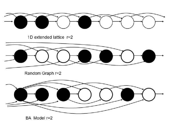
Figure 1: Representation of graphs. Shown is an extended 1D lattice, random graph, and BA model when $r=2$. The white (black) dot is a voter who voted for the candidate $C_{0}(C_{1})$. Two arrows pointing toward a dot represent a voter who refers to two voters when $r=2$. In the case of an extended 1D lattice, a voter refers to the latest two voters. In the case of a random graph, a voter refers to two previous voters who are selected randomly. In the case of the BA model, a voter refers to two previous voters who are selected via connectivity. Hence, there are voters who play the role of a hub in the BA model. In the above figure, the first voter in the network graph is a hub who influences many other voters.

We consider the voter to be able to see $r$ previous votes. The problem becomes one of determining how the voter selects $r$ previous votes. The influence of the reference voters is represented as a voting model on networks. How the network affects the voting model is our problem. In this paper, we analyze cases by comparing models based on a random graph, Barabási-Albert(BA) model case, and fitness model. In Figure 1 we illustrate each one of these three cases for $r=2$. We have previously discussed 1D extended lattice cases and showed that the analog and digital herder cases resemble the Kirman’s ant colony and kinetic Ising models, respectively [24]. In the figure, a white (black) dot is a voter who voted for candidate $C_{0}(C_{1})$. Two arrows point toward a dot, which means a voter refers to two other voters when $r=2$. In the case of the 1D extended lattice, a voter refers to the latest two voters. In the case of a random graph, a voter refers two previous voters who are selected randomly. In the case of the BA model, a voter refers to two previous voters who are selected through the voter’s connectivity network, which is introduced in the BA model [18]. The BA model has the characteristics of a scale-free network with hubs. The power index of the BA model is three, whereas that of the fitness model depends on the distribution of fitness. In the case of a uniform distribution, it is 2.25, which is below three. Hence, there are voters who play the role of a hub to connect other voters. In the above figure, the first voter in the BA model corresponds to a hub.

3 Random Graph

We are interested in the limit $t\rightarrow\infty$. At time $t$, the $t$-th voter selects $r$ voters who have already voted. The $t$-th voter is able to see the total number of votes of selected different $r$ voters to obtain the information. In this section we consider the case in which the voter selects $r$ votes randomly. Hence, this model is a voting model based on the random graph.

Herders vote for a majority candidate as follows. If $c_{0}^{r}(t)>c_{1}^{r}(t)$, the majority of herders vote for the candidate $C_{0}$. If $c_{0}^{r}(t)<c_{1}^{r}(t)$, the majority of herders vote for the candidate $C_{1}$. If $c_{0}^{r}(t)=c_{1}^{r}(t)$, herders vote for $C_{0}$ and $C_{1}$ with the same probability, i.e.,$1/2$. Here at time $t$, the selected information of $r$ previous votes are the number of votes for $C_{0}$ and $C_{1}$, namely $c_{0}^{r}(t)$ and $c^{r}_{1}(t)$, respectively. The herders in this section are known as digital herders.

We define $P_{1}^{r}(t)$ as the probability of the $t$-th voter voting for $C_{1}$.

$$P_{1}^{r}(t)=\begin{cases}p+(1-p)q,\hskip 56.9055pt\,\,\,\,c_{1}^{r}(t)>r/2\\ p/2+(1-p)q,\hskip 45.52458pt\,\,\,\,c_{1}^{r}(t)=r/2\\ (1-p)q,\hskip 78.24507pt\,\,\,\,c_{1}^{r}(t)<r/2\\ \end{cases}$$ (1)

In the scaling limit $t=c_{0}(t)+c_{1}(t)=c_{0}^{\infty}+c_{1}^{\infty}\rightarrow\infty$, we define

$$\frac{c_{1}(t)}{t}=Z(t)\Longrightarrow Z_{\infty}.$$ (2)

$Z(t)$ is the ratio of voters who vote for $C_{1}$ at $t$.

Here we define $\pi$ as the majority probability of binomial distributions of $Z$. In other words, the probability of $c_{1}^{r}(t)>1/2$. When $r$ is odd,

$$\pi(Z)=\sum_{g=\frac{r+1}{2}}^{r}\left(\begin{array}[]{cc}r\\ g\end{array}\right)Z^{g}(1-Z)^{r-g}\equiv\Omega_{r}(Z).$$ (3)

When $r$ is even, from the definition of the behavior of the herder,

$$\pi(Z) = \sum_{g=\frac{r}{2}+1}^{r}\left(\begin{array}[]{cc}r\\ g\end{array}\right)Z^{g}(1-Z)^{r-g}+\frac{1}{2}\left(\begin{array}[]{cc}r\\ r/2\end{array}\right)Z^{g}(1-Z)^{r/2}$$ (8)

$$= \sum_{g=\frac{r}{2}}^{r-1}\left(\begin{array}[]{cc}r-1\\ g\end{array}\right)Z^{g}(1-Z)^{r-1-g}=\Omega_{r-1}(Z).$$ (11)

The majority probability $\pi$ in the even case becomes the odd case $r-1$. Hereafter we consider only the odd case $r=2n+1$, where $n=0,1,2,\dots$.

The value of $\pi$ can be calculated as follows,

$$\pi(Z)=\frac{(2n+1)!}{(n!)^{2}}\int_{0}^{Z}x^{n}(1-x)^{n}dx=\frac{1}{B(n+1,n+1)}\int_{0}^{Z}x^{n}(1-x)^{n}dx.$$ (12)

Equation (12) can be applied when the referred voters are selected to overlap. In fact, in reality the referred voters are not selected to overlap. However, in this paper we use this approximation to study a large $t$ limit.

We can rewrite (1) for the random graph as

$$c_{1}(t) = k\rightarrow k+1:P_{k,t}=p\pi(k/t)+(1-p)q,$$

$$c_{1}(t) = k\rightarrow k:Q_{k,t}=1-P_{k,t},$$ (13)

We define a new variable $\Delta_{t}$ such that

$$\Delta_{t}=2c_{1}(t)-t=c_{1}(t)-c_{0}(t).$$ (14)

We change the notation from $k$ to $\Delta_{t}$ for convenience. Then, we have $|\Delta_{t}|=|2k-t|<t$. Thus, $\Delta_{t}$ holds within $\{-t,t\}$. Given $\Delta_{t}=u$, we obtain a random walk model:

$$\Delta_{t} = u\rightarrow u+1:P_{u,t}=\pi(\frac{1}{2}+\frac{u}{2t})p+(1-p)q,$$

$$\Delta_{t} = u\rightarrow u-1:Q_{u,t}=1-P_{u,t}.$$

We now consider the continuous limit $\epsilon\rightarrow 0$,

$$X_{\tau}=\epsilon\Delta_{[\tau/\epsilon]},$$ (15)

where $\tau=t\epsilon$. Approaching the continuous limit, we can obtain the stochastic differential equation (see Appendix A):

$$\textrm{d}X_{\tau}=[(1-p)(2q-1)-p+2p\frac{(2n+1)!}{(n!)^{2}}\int_{0}^{\frac{1}{2}+\frac{X_{\tau}}{2\tau}}x^{n}(1-x)^{n}dx]\textrm{d}\tau+\sqrt{\epsilon}.$$ (16)

In the case $r=1$, the equation becomes

$$\textrm{d}X_{\tau}=[(1-p)(2q-1)+p\frac{X_{\tau}}{\tau}]\textrm{d}\tau+\sqrt{\epsilon}.$$ (17)

The voters vote for each candidate with probabilities that are proportional to the candidates’ votes. We refer to these herders as a kind of analog herders [21].

We are interested in the behavior at the limit $\tau\rightarrow\infty$. The relation between $X_{\infty}$ and the voting ratio to $C_{1}$ is $2Z-1=X_{\infty}/\tau$. We consider the solution $X_{\infty}\sim\tau^{\alpha}$, where $\alpha\leq 1$, since the maximum speed is $\tau$ when $q=1$. The slow solution is $X_{\infty}\sim\tau^{\alpha}$, where $\alpha<1$ is hidden by the fast solution $\alpha=1$ in the upper limit of $\tau$. Hence, we can assume a stationary solution as

$$X_{\infty}=\bar{v}\tau+(1-p)(2q-1)\tau,$$ (18)

where $\bar{v}$ is constant. Substituting (18) into (16), we can obtain

$$\bar{v}=-p+\frac{2p\cdot(2n+1)!}{(n!)^{2}}\int_{0}^{\frac{1}{2}+\frac{(1-p)(2q-1)}{2}+\frac{\bar{v}}{2}}x^{n}(1-x)^{n}dx.$$ (19)

This is the self-consistent equation.

Equation (19) admits one solution below the critical point $p\leq p_{c}$ and three solutions for $p>p_{c}$. When $p\leq p_{c}$, we refer to the phase as the one-peak phase. When $p>p_{c}$, the upper and lower solutions are stable; on the other hand, the intermediate solution is unstable. Then, the two stable solutions correspond to good and bad equilibria, respectively, and the distribution becomes the sum of the two Dirac measures. We refer to this phase as a two-peaks phase.

If $r=2n+1\geq 3$, a phase transition occurs in the range $0\leq p\leq 1$. If the voter obtains information from three of the above voters, as the number of herders increases, the model features a phase transition beyond which the state in which most voters make the correct choice coexists with one in which most of them are wrong. If the voter only obtains information from one or two other voters, there is no phase transition. We refer to this transition as an information cascade transition [15].

Next, we consider the phase transition resulting from convergence. This type of transition has been studied for analog herders [21]. We expand $X_{\tau}$ around the solution $\bar{v}\tau+(1-p)(2q-1)\tau$.

$$X_{\tau}=\bar{v}\tau+(1-p)(2q-1)\tau+W_{\tau}.$$ (20)

Here, we set $X_{\tau}\gg W_{\tau}$, that is $\tau\gg 1$. We rewrite (16) using (20) and obtain the following:

$$\textrm{d}W_{\tau} = p\frac{(2n+1)!}{(n!)^{2}\cdot 2^{2n}}\frac{W_{\tau}}{\tau}[1-\{\bar{v}+(1-p)(2q-1)\}^{2}]^{n}\textrm{d}\tau+\sqrt{\epsilon}.$$ (21)

We use relation (18) and consider the first term of the expansion. If we set $L=p(2n+1)!/\{(n!)^{2}\cdot 2^{2n}\}[1-\{\bar{v}+(1-p)(2q-1)\}^{2}]^{n}$, then (53) is identical to (21).

The phase transition of convergence is obtained from the explanation in Appendix B. The critical point $p_{vc}$ is the solution of

$$p\frac{(2n+1)!}{(n!)^{2}\cdot 2^{2n}}[1-\{\bar{v}+(1-p)(2q-1)\}^{2}]^{n}=\frac{1}{2},$$ (22)

and the self-consistent equation (19).

Here we consider the symmetric case, $q=1/2$. The self-consistent equation (19) becomes

$$\bar{v}=-p+\frac{2p\cdot(2n+1)!}{(n!)^{2}}\int_{0}^{\frac{1}{2}+\frac{\bar{v}}{2}}x^{n}(1-x)^{n}dx.$$ (23)

The right-hand side (RHS) of (23) rises at $\bar{v}=0$. If $r=1,2$, there is only one solution $\bar{v}=0$ in all regions of $p$. In this case, $Z$ only has one peak, at $0.5$, which indicates the one-peak phase. In the case $r=1,2$, we do not observe an information cascade transition [15]. On the other hand, in the case $r\geq 3$, there are two stable solutions and an unstable solution $\bar{v}=0$ above $p_{c}$. The votes ratio for $C_{1}$ attains a good or bad equilibrium. This is the so-called spontaneous symmetry breaking. In one sequence, $Z$ is taken as $\bar{v}/2+1/2$ in the case of a good equilibrium, or as $-\bar{v}/2+1/2$ in the case of a bad equilibrium, where $\bar{v}$ is the solution of (23). This indicates the two-peaks phase, and the critical point is $p_{c}=\frac{(n!)^{2}}{(2n+1)!}2^{2n}$, where the gradient of the RHS of (23) at $\bar{v}=0$ is $1$. In the case of $r=3(n=1)$, $p_{c}=2/3$ and $r=5(n=2)$, $p_{c}=8/15$. As $r$ increases, $p_{c}$ moves towards $0$. In the large limit $r\rightarrow\infty$, $p_{c}$ becomes $0$. This is consistent with the case in which herders obtain information from all previous voters.[25]

Next, we consider the normal-to-super transition of the symmetric case $q=1/2$ by considering the case $r=2n+1\geq 3$. In this case, we observe an information cascade transition. If $r\leq 2$, we do not observe an information cascade transition and we can only observe a part of the phases, as described below.

In the one-peak phase $p\leq p_{c}$, the only solution is $\bar{v}=0$. $p_{c}$ is the critical point of the information cascade transition. The first critical point of convergence is $p_{vc1}=\frac{(n!)^{2}}{(2n+1)!}2^{2n-1}=\frac{p_{c}}{2}$. When $p\leq p_{c}$, $p_{vc1}$ is the solution of (23) and (22). If $0<p<p_{vc1}$, the voting rate for $C_{1}$ becomes $1/2$, and the distribution converges as in a binomial distribution. If $p_{c}>p\geq p_{vc1}$, candidate $C_{1}$ gathers $1/2$ of all the votes, also in the scaled distributions. However, the rate at which the voting rate converges is lower than in a binomial distribution. We refer to these phases as super diffusion phases. There are two phases, $p=p_{vc1}$ and $p_{c}>p>p_{vc1}$ and they differ in terms of their convergence speed. If $r\leq 2$, we can observe these three phases.

Above $p_{c}$, in the two-peaks phase, we can obtain two stable solutions that are not $\bar{v}=0$. At $p_{c}$, $\bar{v}$ moves from $0$ to one of these two stable solutions. In one voting sequence, the votes converge to one of these stable solutions. If $p_{c}<p\leq p_{vc2}$, the voting rate for $C_{1}$ becomes $\bar{v}/2+1/2$ or $-\bar{v}/2+1/2$, and the convergence occurs at a lower rate than in a binomial distribution. Here, $\bar{v}$ is the solution of (23). We refer to this phase as a super diffusion phase. $p_{vc2}$ is the second critical point of convergence from the super to the normal diffusion phase, and it is the solution of the simultaneous equations (23) and (22) when $p>p_{c}$. In the case $r=3$ we can obtain $p_{vc2}=5/6$ at $\bar{v}=\pm\sqrt{(3p-2)/p}$. If $p>p_{vc2}$, the voting rate for $C_{1}$ becomes $\bar{v}/2+1/2$ or $-\bar{v}/2+1/2$. However, the distribution converges as in a binomial distribution. This is a normal diffusion phase. A total of six phases can be observed.

4 Barabási-Albert model

In this section we consider the case in which the voter selects $r$ different voters who will be selected based on popularity. The popularity is proportional to the connectivity of the voter $i$, such that $l_{i}/\sum_{j}l_{j}$, where $l_{i}$ is the sum of the number of voters whom voter $i$ gave the information and from whom voter $i$ obtained information, referenced against $r$ voters. The total number of $l_{i}$ after the $t$-th voter has voted is $\sum_{j}l_{j}=2r(t-r+1)$, where $t\geq r$. The sum $l_{i}$ corresponds to the connectivity in the BA model [18]. Hence, this model is the voting model based on the BA model. The difference in the connectivity is represented by different colors. The color depends on whether the voter voted for candidate $C_{1}$ or $C_{0}$. In Figure 2, voters who voted for $C_{1}$($C_{0}$) are represented by black(white) circles. We define the total connectivity number of voters who voted for candidate $C_{1}$($C_{0}$) at $t$ as $g_{1}(t)$($g_{0}(t)$). Hence, $g_{0}(t)+g_{1}(t)=2r(t-r+1)$, where $t\geq r$. In the scaling limit $g_{0}(t)+g_{1}(t)=2r(t-r+1)\rightarrow\infty$, we define

$$\frac{g_{1}(t)}{2r(t-r+1)}=\hat{Z}(t)\Longrightarrow\hat{Z}_{\infty},$$ (24)

$\hat{Z}(t)$ is $g_{1}(t)/2r(t-r+1)$ at $t$.

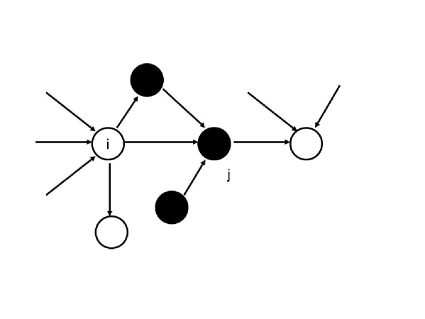
Figure 2: The sample graph BA model with $r=3$. The voter $i$, who refers three voters and is referred by three voters, is represented by a white circle, because they voted for candidate $C_{0}$. The connectivity of $i$ is six. The voter $j$ refers three voters and is referred by a voter and is represented by a black circle, because of voting for candidate $C_{1}$. The connectivity of $j$ is four.

We can write the evolution of connectivity as

$$g_{1}(t)=\hat{k}\rightarrow\hat{k}+i:$$

$$(3r+1)/2\leq i\leq 2r P_{\hat{k},t}(i)={}_{r}C_{2r-i}\hat{Z}^{i-r}(1-\hat{Z})^{2r-i}[(1-p)q+p],$$

$$r+1\leq i\leq(3r-1)/2 P_{\hat{k},t}(i)={}_{r}C_{2r-i}\hat{Z}^{i-r}(1-\hat{Z})^{2r-i}(1-p)q,$$

$$i=r P_{\hat{k},t}(i)=(1-\hat{Z})^{r}(1-p)q+\hat{Z}^{r}(1-p)(1-q),$$

$$(r+1)/2\leq i\leq r-1 P_{\hat{k},t}(i)={}_{r}C_{r-i}\hat{Z}^{i}(1-\hat{Z})^{r-i}(1-p)(1-q),$$

$$0\leq i\leq(r-1)/2 P_{\hat{k},t}(i)={}_{r}C_{r-i}\hat{Z}^{i}(1-\hat{Z})^{r-i}[(1-p)(1-q)+p].$$

Here we consider the self-consistent equations for connectivity at a large $t$ limit.

$$2r\hat{Z}_{\infty}=\sum_{i=1}^{2r}P_{\hat{k},t}(i)\cdot i=r(1-p)q+rp\pi(\hat{Z}_{\infty})+r\hat{Z}_{\infty}.$$ (26)

Hence, we can obtain

$$\hat{Z}_{\infty}=(1-p)q+p\pi(\hat{Z}_{\infty}).$$ (27)

On the other hand, the evolution equation for the voting ratio $Z_{\infty}$ is

$$Z_{\infty}=(1-p)q+p\pi(\hat{Z}_{\infty}).$$ (28)

Comparing (27) and (28), we can obtain $Z_{\infty}\sim\hat{Z}_{\infty}$. It means the behavior of the voting ratio, $Z_{\infty}$ is the same as that of the connectivity ratio, $\hat{Z}_{\infty}$. Hereafter, we only analyze the behavior of the connectivity.

We define a new variable $\hat{\Delta}_{t}$ such that

$$\hat{\Delta}_{t}=g_{1}(t)-r(t-r+1)=\frac{1}{2}\{g_{1}(t)-g_{0}(t)\}.$$ (29)

We change the notation from $\hat{k}$ to $\hat{\Delta}_{t}$ for convenience. Thus, $\hat{\Delta}_{t}$ holds within $\{-r(t-r+1),r(t-r+1)\}$. Given $\hat{\Delta}_{t}=\hat{u}$, we obtain a random walk model:

$$\hat{\Delta}=\hat{u}\rightarrow\hat{u}+i:$$

$$(r+1)/2\leq i\leq r P_{\hat{u},t}(i)={}_{r}C_{r-i}\hat{Z}^{i}(1-\hat{Z})^{r-i}[(1-p)q+p],$$

$$1\leq i\leq(r-1)/2 P_{\hat{u},t}(i)={}_{r}C_{r-i}\hat{Z}^{i}(1-\hat{Z})^{r-i}(1-p)q,$$

$$i=0 P_{\hat{u},t}(i)=(1-\hat{Z})^{r}(1-p)q+\hat{Z}^{r}(1-p)(1-q),$$

$$(-r+1)/2\leq i\leq-1 P_{\hat{u},t}(i)={}_{r}C_{-i}\hat{Z}^{r+i}(1-\hat{Z})^{-i}(1-p)(1-q),$$

$$-r\leq i\leq-(r+1)/2 P_{\hat{u},t}(i)={}_{r}C_{-i}\hat{Z}^{r+i}(1-\hat{Z})^{-i}[(1-p)(1-q)+p],$$

where $\hat{Z}=\hat{k}/(2r(t-r+1))=\hat{u}/(2r(t-r+1))+1/2$.

We now consider the continuous limit $\epsilon\rightarrow 0$,

$$\hat{X}_{\tau}=\epsilon\hat{\Delta}_{[\tau/\epsilon]},$$ (31)

where $\tau=t\epsilon$. Approaching the continuous limit, we can obtain the stochastic partial differential equation (see Appendix A):

$$\textrm{d}\hat{X}_{\tau} = [r(1-p)q-\frac{r}{2}+\frac{\hat{X}_{\tau}}{2(\tau-r+1)}$$ (32)

$$+rp\frac{(2n+1)!}{(n!)^{2}}\int_{0}^{\frac{1}{2}+\frac{\hat{X}_{\tau}}{2r(\tau-r+1)}}x^{n}(1-x)^{n}dx]\textrm{d}\tau+\sqrt{\epsilon}.$$

For $r=1$, the equation becomes

$$\textrm{d}\hat{X}_{\tau}=[(1-p)(q-\frac{1}{2})+\frac{p+1}{2}\frac{\hat{X}_{\tau}}{\tau}]\textrm{d}\tau+\sqrt{\epsilon}.$$ (33)

The voters also vote for each candidate with probabilities that are proportional to $\hat{X}_{\tau}$. However, equation (33) is different from (17). The relation between the voting ratio for $C_{1}$ and $\hat{X}_{\infty}$ is

$$\frac{\hat{X}_{\infty}}{2r(\tau-r+1)}=\hat{Z}_{\infty}-\frac{1}{2}.$$ (34)

We can assume a stationary solution as

$$\hat{X}_{\infty}=r\bar{\hat{v}}\tau+r(1-p)(2q-1)\tau,$$ (35)

where $\bar{\hat{v}}$ is constant. Since (34) and $0\leq\hat{Z}\leq 1$, we can obtain

$$-1\leq\bar{\hat{v}}+(1-p)(2q-1)\leq 1.$$ (36)

Substituting (35) into (32), we can obtain

$$\bar{\hat{v}}=-p+\frac{2p\cdot(2n+1)!}{(n!)^{2}}\int_{0}^{\frac{1}{2}+\frac{(1-p)(2q-1)}{2}+\frac{\bar{\hat{v}}}{2}}x^{n}(1-x)^{n}dx.$$ (37)

This is the self-consistent equation and it agrees with (19). Then, in the BA model the information cascade transition behaves the same as in the random graph case. When $p\leq p_{c}$, we refer to the phase as the one-peak phase. Equation (37) admits three solutions for $p>p_{c}$. When $p>p_{c}$, the upper and lower solutions are stable; on the other hand, the intermediate solution is unstable. The two stable solutions correspond to good and bad equilibria, respectively, and the distribution becomes the sum of the two Dirac measures. This is the two-peaks phase. The phase transition point $p_{c}$ in the case of the BA model is the same as that in the random graph case. If $r=2n+1\geq 3$, a phase transition occurs in the range $0\leq p\leq 1$. If the voter obtains information from either one or two voters, there is no phase transition.

Next, we consider the phase transition of convergence. We expand $\hat{X}_{\tau}$ around the solution $r\bar{\hat{v}}\tau+r(1-p)(2q-1)\tau$.

$$X_{\tau}=r\bar{\hat{v}}\tau+r(1-p)(2q-1)\tau+r\hat{W}_{\tau}.$$ (38)

Here, we set $X_{\tau}\gg W_{\tau}$. This indicates $\tau\gg 1$. We rewrite (33) using (38) and obtain the following:

$$\textrm{d}\hat{W}_{\tau} = [1+p\frac{(2n+1)!}{(n!)^{2}\cdot 2^{2n}}(1-\{\bar{\hat{v}}+(1-p)(2q-1)\}^{2})^{n}]\frac{W_{\tau}}{2\tau}\textrm{d}\tau+\sqrt{\epsilon}.$$ (39)

We use relation (37) and consider the first term of the expansion. If we set $L=1/2[1+p(2n+1)!/\{(n!)^{2}\cdot 2^{2n}\}(1-\{\bar{\hat{v}}+(1-p)(2q-1)\}^{2})^{n}]$, (53) is identical to (39).

From Appendix B, we can obtain the phase transition of convergence. The critical point $p_{vc}$ is the solution of

$$[1+p\frac{(2n+1)!}{(n!)^{2}\cdot 2^{2n}}(1-\{\bar{\hat{v}}+(1-p)(2q-1)\}^{2})^{n}]\frac{1}{2}=\frac{1}{2},$$ (40)

and (37). The RHS of (40) is not less than $1/2$. Using (36) we can obtain $p_{vc}=0$. There is no normal phase in the case of the BA model. The speed of convergence is always lower than normal in all regions of $p$.

5 Fitness model

In this section we consider the fitness model, which includes the BA model [19], [20]. We set the fitness of each voter equal to the weight of the connectivity. When the fitness has a constant distribution, the fitness model becomes the BA model. These models lead to the appearance of stronger hubs. The problem is whether the stronger hubs affect the phase transition points $p_{c}$ and $p_{vc}$.

The popularity is proportional to the weighted connectivity of voter $i$, such that $\eta_{i}l_{i}/\sum_{j}\eta_{j}l_{j}$, where $l_{i}$ is the sum of the number of voters to whom voter $i$ gave the information and from whom voter $i$ obtained information, referenced against $r$ voters. Further, $\eta_{i}$ is the fitness of voter $i$ and it is chosen from the distribution $u$. The total number of weighted $l_{i}$ after the $t$-th voter has voted is $\sum_{j}l_{j}=2r(t-r+1)\bar{\eta}$, where $t\geq r$ and $\bar{\eta}$ is the average of the fitness. When $u$ is a constant distribution, the fitness model becomes the BA model. In the next section we discuss the cases for which the distribution of $\eta$ is constant, and uniform and exponential distributions for numerical simulations. We define the total number of weighted connectivity of the voters who voted for candidate $C_{1}$($C_{0}$) at $t$ as $g_{1}(t)$($g_{0}(t)$). Hence, $g_{0}(t)+g_{1}(t)=2r\bar{\eta}(t-r+1)$, where $t\geq r$. In the scaling limit $g_{0}(t)+g_{1}(t)=2\bar{\eta}r(t-r+1)\rightarrow\infty$, we define

$$\frac{g_{1}(t)}{2r\bar{\eta}(t-r+1)}\Longrightarrow\hat{Z}_{\infty},$$ (41)

where $\hat{Z}(t)$ is $g_{1}(t)/2r\bar{\eta}(t-r+1)$ at $t$.

Here we consider the self-consistent equations for connectivity in the large $t$ limit. We set the condition under which voter $i$ votes and $\hat{Z}_{\infty}$ does not change as equilibrium. Using (13) we obtain:

$$r\bar{\eta}\hat{Z}_{\infty}+r\eta_{i}\hat{Z}_{\infty}=r(1-p)q\eta_{i}+rp\pi(\hat{Z}_{\infty})\eta_{i}+r\bar{\eta}\hat{Z}_{\infty}.$$ (42)

Hence, we can obtain

$$\hat{Z}_{\infty}=(1-p)q+p\pi(\hat{Z}_{\infty}).$$ (43)

which is the same as (27). This means that the transition point $p_{c}$ of the fitness model is that same as that of the BA model, for which there is no super-normal transition. From this result, we can estimate that there is no super-normal transition for the fitness models, details of which are discussed in the next section.

6 Numerical Simulations

In this section, we present a study of the voting model using several kinds of networks for which we use a numerical method. As fitness models, we consider three types of networks, which are constructed based on the mechanism of preferential attachment of nodes. The type of the degree distribution is determined by the distribution $u$ of the fitness $\eta$ of each node. We denote the networks C,U, and E, as the distribution $u$ is Constant, obeys Uniform distribution, and obeys Exponential distribution. C corresponds to the BA model. In addition, we also study the voting models in a Random graph and a 1D extended Lattice. We name the networks L and R, respectively, and adopt the model parameters $(r,q,p)$ as $r\in\{3,9\},q\in\{0.5,0.8\}$ and change the control parameter $p\in[0,1]$. We performed Monte Carlo simulations for time horizon $T$ as $T=3.2\times 10^{4}$ and gathered $10^{5}$ samples. We calculated the average values of the macroscopic quantities with $S=10^{2}$ network samples.

The fitness model contains a phase transition similar to a Bose-Einstein (BE) condensation [20]. The BE condensation represents a ”winner-takes-all” phenomenon for networks; in other words, a few voters play the role of a large hub. The cases C and U correspond to a scale-free phase and the case E corresponds to a BE condensation phase.

6.1 Convergence of $Var(Z)$

Figure 3 shows the simulations performed for the symmetric independent voter case, i.e., $q=1/2$. Convergence of distribution is observed in the C, U, E, L, and R cases for the symmetric case $q=1/2$. MF is the theoretical line obtained in the previous sections. The reference number is $r=3$ and $r=9$. Cases $q=0.5$ and $q=0.8$ represent independent voters. The horizontal axis represents the ratio of herders $p$, and the vertical axis represents the speed of convergence $\gamma$. We define $\gamma$ as $Var(Z)=\tau^{-\gamma}$, where $Var(Z)$ is the variance of $Z$. Here, $\gamma=1$ is the normal phase and $0<\gamma<1$ is the super diffusion phase.

As discussed in the previous sections, the critical point at which the transition converges from normal diffusion to super diffusion is $p_{vc}\sim 0$ for the C, U, and E cases. This means there is no normal phase for these cases. These models only have a super phase because of the hubs. The case $L$ also does not have a phase transition from super to normal and only has a normal phase. On the other hand, we can observe a phase transition from super to normal in the R case.

At the critical point of the information cascade transition, the distribution splits into two delta functions and the exponent $\gamma$ becomes $0$. For the C, U, E, and R cases, the critical point $p_{c}$ seems to be the same. In the L case, there is no information cascade transition [24]. In the next subsection, we discuss phase transitions from the viewpoint of scaling.

.

Figure 3: Plot $\gamma$ vs. $p$. $q=0.5,r=3$ (Top Left),$q=0.5,r=9$ (Top Right),$q=0.8,r=3$ (Bottom Left) and $q=0.8,r=9$ (Bottom Right). $t=3.2\times 10^{4}$. C($\Box$),U($\bigcirc$),E($\bigtriangleup$),R$(\bigtriangledown)$ and L($\diamond$). The solid and dotted lines show the theoretical results of mean-field approximations for the R and C cases.

6.2 Estimator for $l$ and Var$(Z)$

The phase transition of the voting models was detected by considering that the normalized correlation function $C(t)$ between the first voter’s choice and $(t+1)$-th voter’s choice plays a key role[26],[27]. The function is defined as the covariance divided by the variance of the first voter’s choice. The asymptotic behavior of $C(t)$ depends on the phase of the system and the expansion coefficient $l$. In the one-peak phase, the leading term of $C(t)$ shows a power law dependence on $t$ as $t^{l-1}$. In the two-peaks phase, the limit value $c\equiv\lim_{t\to\infty}C(t)$ is positive and plays the role of the order parameter of the information cascade phase transition. The sub-leading term depends on $t$ as $t^{l-1}$ and $l$ is the larger value $l_{max}$ of the two expansion coefficients $\{l_{+},l_{-}\}$ at the two peaks. We summarize the asymptotic behavior of $C(t)$ as

$$C(t)\simeq\begin{cases}a\cdot t^{l-1},\,\,\,\,c=0\\ c+a\cdot t^{l-1},\,\,\,\,c>0.\end{cases}$$ (44)

Here, we write the coefficient of the term proportional to $t^{l-1}$ as $a$. $c$ is equal to the limit value of $\lim_{t\to\infty}\mbox{Var}(Z(t))$ divided by the variance of the first voter’s choice. On the phase boundary between the one-peak and two-peaks phase, the result for a generalized Pólya urn process suggests the following asymptotic behavior [27].

$$C(t)\simeq c+a\cdot\log t^{-\alpha}+o(\log t^{-\alpha}).$$ (45)

For the (a)symmetric case $q=\frac{1}{2}(\neq\frac{1}{2})$, $c=0(>0)$ and $\alpha\simeq\frac{1}{2}(1)$.

To estimate $c$ and $l$, the integrated correlation time $\tau(t)$ and the second-moment correlation length $\xi(t)$ are useful. The values of the latter two parameters are defined through the $n$-th moment of $C(t)$ as,

$$\tau(t)\equiv M_{0}(t)\,\,\,\,,\,\,\,\,\xi(t)\equiv\sqrt{\frac{M_{n}(t)}{M_{0}(t)}}\,\,\,\,,\,\,\,\,M_{n}(t)\equiv\sum_{s=0}^{t-1}C(s)s^{n}.$$ (46)

We estimate the limit value of $\xi_{t}(t)\equiv\xi(t)/t$ and $\tau_{t}(t)\equiv\tau(t)/t$ using the asymptotic behavior of $C(t)$ in eq.(44) as

$$\lim_{t\to\infty}\tau_{t}(t)=\lim_{t\to\infty}c+\frac{a}{l}t^{l-1}=c\,\,\,\,,\,\,\,\,\lim_{t\to\infty}\xi_{t}(t)=\begin{cases}\sqrt{\frac{l}{l+2}},\,\,\,\,c=0\\ \sqrt{\frac{1}{3}},\,\,\,\,c>0.\end{cases}$$ (47)

We can determine the one-peak phase or two-peaks phase by the limit value of $\tau_{t}(t)$. In the one-peak phase, the limit value $\lim_{t\to\infty}\xi_{t}(t)$ can be used to estimate $l$. On the phase boundary and in the two-peaks phase $l=1$.

6.3 Order parameter $c$

Figure 4: Plot $\tau_{t}(t)$ vs. $p$. $q=0.5,r=3$ (Top Left),$q=0.5,r=9$ (Top Right),$q=0.8,r=3$ (Bottom Left) and $q=0.8,r=9$ (Bottom Right). $t=3.2\times 10^{4}$. C($\Box$),U($\bigcirc$),E($\bigtriangleup$),R$(\bigtriangledown)$ and L($\diamond$). The broken line shows the position of $p_{c}(q,r)$ for each case. For the C, U, E, and R cases, $p_{c}(q,r)$ is the same. In the L case, there is no phase transition.

We estimate $\tau_{t}(t)$ for $t=T=3.2\times 10^{5}$ as a function of $p$ for C, U, E, R, and L. The results for $r\in\{3,9\}$ and $q\in\{0.5,0.8\}$ are plotted in Figure 4.

In the case L, $p_{c}=1$ and $\tau_{t}(t)$ is almost zero for $p<1$ and becomes 1 at $p=1$. In other cases, $\tau_{t}(t)$ becomes an increasing function of $p$. The broken line shows the common position of $p_{c}$ in (19) and (37) for C, U, E, and R. If $p>p_{c}$, $\tau(t)/t$ is positive for $t=3.2\times 10^{4}$. If $p$ is sufficiently small and $p<p_{c}$, $\tau(t)/t$ is almost zero. In the region $p\simeq p_{c}$ and for $p<p_{c}$, the limit value $\lim_{t\to\infty}\tau_{t}(t)$ should be zero as the system is in the one-peak phase. However, as can clearly be seen, the finite-size corrections are large and $\tau_{t}(t)$ assumes a large positive value. To see the limit $\lim_{t\to\infty}\tau_{t}(t)$ it is necessary to study the scale transformation $t\to\sigma t$ and the limit $\sigma\to\infty$. The plots of $\tau_{t}(t)$ suggest that the value of $p_{c}$ is equal for C, U, E, and R.

On the phase boundary $p=p_{c}$, the situation is subtle and requires further careful study to examine the limit value of $\tau_{t}(t)$. We think that the decrease of $\tau_{t}(t)$ with $t$ obeys a power law of $\log t$ as in eq.(45). A naïve extrapolation of the numerical results are not expected to work and it may be necessary to use finite-size scaling analysis to study the limit.

6.4 Exponent $l$ in the one-peak phase

We calculate $\xi(t)$ for $t=T$ and estimate $l$ by using the relation $\lim_{t\to\infty}\xi_{t}(t)=\sqrt{l/l+2}$. $l$ determines whether the system is in the one-peak phase or the two-peaks phase by the condition $l<1$ or $l=1$. Furthermore, it also uses the condition $l>1/2$ or $l<1/2$ to determine whether the system is super-diffusive or normal diffusive.

As $\tau(t)\simeq ct+\frac{a}{l}t^{l}$ from eq.(47), one can derive the scaling relation for $\tau(t)$ under the scale transformation $t\to\sigma t$ as

$$\frac{\tau(\sigma t)}{\tau(t)}=\sigma^{l}.$$ (48)

In the two-peaks phase, we adopt $l=1$ in the relation. Under the scale transformation, $\tau_{t}(t)$ does not change and the limit value $\lim_{t\to\infty}\tau_{t}(t)$ is positive if it is positive for sufficiently large $t$. In the one-peak phase, $l<1$ and the limit value of $\tau_{t}(t)$ vanishes.

Figure 5: Plot of $\log_{2}\tau(2t)/\tau(t)$ vs. $l$. $2t=T$,$(r,q)\in\{(3,0.5),(9,0.8)\}$ and C,U,E,and R networks.

Figure 5 plots the logarithm of $\tau(2t)/\tau(t)$ with $2t=T$ as function of $l$. We use the data for $(r,q)\in\{(3,0.5),(9,0.8)\}$ and C,U,E,and R networks. One sees that the data lie on the diagonal and the relation (48) holds for the models in the C,U,E, and R networks. About L, $\tau(t)$ obeys another scaling relation [26].

Figure 6: Plot of $l$ estimated by $\xi_{t}(t)=\sqrt{l/(l+2)}$. The solid and dotted lines show the results of mean-field theory for $l_{max}$ in C and R networks, respectively. The broken line shows the position of $p_{c}$ for each case. The parameters selections and the symbols are the same as those in Figure 4.

Figure 6 plots $l$ as a function of $p$. In L with $r=3$, $l=0$ for $p<p_{c}=1$ and the system is in the one-peak phase. $\tau_{t}$ are vanishingly small for $p<1$. For $p\simeq 1$ with $r=9$, $l$ has a large positive value and touches 1 at $p<1$. This is an artefact of the finite-size correction. If one estimates $l$ by using the large $T$ data, it should vanish for $p<1$.

The broken line shows the common position of $p_{c}$ for C, U, E, and R networks. We also plotted the theoretical results for $l$ in (19),(37) by using thin solid and dotted lines for the C and R networks. If $p>p_{c}$, $l$ is 1 and the systems are in the two-peaks phase. If $p<p_{c}$, $l$ is less than 1 and it is in the one-peak phase. The theoretical results for $l_{max}$ provide a good description of the behavior of $l$ in the one-peak phase.

For $q=0.5$ and C, $l$ is always larger than $0.5$ for $p>0$ and the system is in the super-diffusive phase. In case R, $l$ changes continuously from 0 to 1 with $p$, which suggests the normal-diffusive phase transition. For $q=0.8$, one see some discrepancy between the two estimates of $l$. It suggests that the time horizon $T=3.2\times 10^{4}$ is insufficiently large, preventing the system from reaching the scaling region. In case C with $r=3$, $l>1/2$, which means that the system might be in the super-diffusive phase for $p>0$. In case C with $r=9$, we cannot deny the normal-diffusive phase with $l<0.5$. As the finite-size correction is large for case R, we cannot deny the super-diffusive phase between the one-peak normal-diffusive phase and the two-peaks phase. For U and E, the plots confirm that $p_{c}$ is common with C and R. As $l$ for U and E is always larger than that of C, the system might be in the one-peak super-diffusive phase for $p<p_{c}$.

7 Concluding Remarks

In this paper we present a voting model with collective herding behavior for the random graph, BA model, and fitness model cases. We investigated the phase differences between three different networks as models for the source of voter information. This is based on the consideration that voters obtain their information from a network including hubs. The BA and fitness models have networks that are similar to real networks with hubs. At the continuous limit, we could obtain stochastic differential equations, which were subsequently used to analyze the difference between the models.

Our proposed model uses two kinds of phase transitions, one of which is the information cascade transition. As the number of herders increased, the model featured a phase transition beyond which a state in which most voters make the correct choice coexisted with one in which most of them are wrong. At this transition, the distribution of votes changed from the one-peak phase to the two-peaks phase.

The other phase transition occurred at the convergence of the super and normal diffusions. In the one-peak phase, a decrease in the number of herders caused the rate at which the variance converged to be slower than in the binomial distribution. This is the transition from normal diffusion to super diffusion. This transition was also found in the two-peaks phase, in which sequential voting converged to one of the two peaks.

In the case of the random graph model, all of these phases can be observed. However, in the case of the BA and fitness models, it is only possible to observe the super phase in the one-peak and two-peaks phases. On the other hand, in the case of the 1D extended lattice phase, the only phase that exists is the one-peak phase, which represents a normal convergence without any phase transition [24].

The critical point $p_{c}$ is the same, regardless of whether the random graph, BA, or fitness models are used. However, the difference can be observed in the normal and super phases. In the case of the BA model, there is only a super phase of which the convergence speed is slower than for the normal phase. In the case of the random network model, the super phase and normal phase coexist. The fitness model, which has stronger hubs than the BA model, has the same phase as the BA model. In conclusion, the influence of hubs can only be seen in the convergence speed and cannot be seen in the phase transition between the one-peak and two-peaks phases.

In [22] the ”influential hypothesis” was discussed and negative opinions were expressed. The hypothesis holds that influence, i.e., the existence of hubs, is important for the formation of public opinion. In our model the network does not affect the critical point at which an information cascade transition occurs. In this work hubs are only affected by the critical point of super-normal transitions for a large $t$ limit. The phase transition is the transition of the speed of convergence. Hence, although the existence of hubs affects the standard deviation of the votes, they are unable to change the final outcome. Therefore, we can conclude that a hub has limited influence.

In this paper we discussed the case that herders’ threshold is one half, i.e., that there is an equal probability of herders voting for either one of two candidates. To confirm our conclusions, we will make a two-choice quiz experiment on networks which is similar to [23]. In the real world, the threshold is not a half. We discussed the bunk run case of Toyokawa Credit Union [16], [17]. In this case we are required to go to a bank without immediate confirmation. Because we are sensitive about rumors such as this, the threshold is reduced to much below a half. In next paper, we plan to study the case for which the threshold is a variable and compare to observations [10], [11].

Considering the intermediate case between a 1D extended lattice and a random network, in the previous paper, we showed that a 1D extended lattice is characterized by the absence of a phase transition and the presence of a one-peak phase [24]. In contrast, a random network has both information cascade and super-normal transitions. Investigating intermediate phases would be an interesting problem. These networks are nothing but small-world networks [28]. Investigation of a voting model on a small-world network is a future problem.

Appendix Appendix A Derivation of stochastic differential equation

We use $\delta X_{\tau}=X_{\tau+\epsilon}-X_{\tau}$ and $\zeta_{\tau}$, a standard i.i.d. Gaussian sequence with the objective to identify the drift $f_{\tau}$ and the variance $g^{2}_{\tau}$ such that

$$\delta X_{\tau}=f_{\tau}(X_{\tau})\epsilon+\sqrt{\epsilon}g_{\tau}(X_{\tau})\zeta_{\tau+\epsilon}.$$ (49)

Given $X_{\tau}=x$, using the transition probabilities of $\Delta_{n}$, we obtain

$$\textrm{E}(\delta X_{\tau}) = \epsilon\textrm{E}(\Delta_{[\tau/\epsilon]+1}-\Delta_{[\tau/\epsilon]})=\epsilon(2p_{[\frac{l/\epsilon+\tau/\epsilon}{2}],\tau/\epsilon}-1)$$ (50)

$$= \epsilon[(1-p)(2q-1)-p+2p\frac{(2n+1)!}{(n!)^{2}}\int_{0}^{\frac{1}{2}+\frac{X_{\tau}}{2\tau}}x^{n}(1-x)^{n}dx].$$

Then, the drift term is $f_{\tau}(x)=(1-p)(2q-1)+p\tanh(\lambda x/2\tau)$. Moreover,

$$\sigma^{2}(\delta X_{\tau})=\epsilon^{2}[1^{2}p_{[\frac{l/\epsilon+\tau/\epsilon}{2}],\tau/\epsilon}+(-1)^{2}(1-p_{[\frac{l/\epsilon+\tau/\epsilon}{2}],\tau/\epsilon})]=\epsilon^{2},$$ (51)

such that $g_{\epsilon,\tau}(x)=\sqrt{\epsilon}.$ We can obtain $X_{\tau}$ such that it obeys a diffusion equation with small additive noise:

$$\textrm{d}X_{\tau}=[(1-p)(2q-1)-p+2p\frac{(2n+1)!}{(n!)^{2}}\int_{0}^{\frac{1}{2}+\frac{X_{\tau}}{2\tau}}x^{n}(1-x)^{n}dx]\textrm{d}\tau+\sqrt{\epsilon}.$$ (52)

Appendix Appendix B Behavior of solutions of the stochastic differential equation

We consider the stochastic differential equation

$$\textrm{d}x_{\tau}=(\frac{Lx_{\tau}}{\tau})\textrm{d}\tau+\sqrt{\epsilon},$$ (53)

where $\tau\geq 1$.

Let $\sigma^{2}_{1}$ be the variance of $x_{1}$. If $x_{1}$ is Gaussian $(x_{1}\sim\textrm{N}(x_{1},\sigma^{2}_{1}))$ or deterministic $(x_{1}\sim\delta_{x1})$, the law of $x_{\tau}$ ensures that the Gaussian is in accordance with density

$$p_{\tau}(x)\sim\frac{1}{\sqrt{2\pi}\sigma_{\tau}}\textrm{e}^{-(x-\mu_{\tau})^{2}/2\sigma_{\tau}^{2}},$$ (54)

where $\mu_{\tau}=\textrm{E}(x_{\tau})$ is the expected value of $x_{\tau}$ and $\sigma^{2}_{\tau}\equiv\nu_{\tau}$ is its variance. If $\Phi_{\tau}(\xi)=\log(\textrm{e}^{\textrm{i}\xi x_{\tau}})$ is the logarithm of the characteristic function of the law of $x_{\tau}$, we have

$$\partial_{\tau}\Phi_{\tau}(\xi)=\frac{L}{\tau}\xi\partial_{\xi}\Phi_{\tau}(\xi)-\frac{\epsilon}{2}\xi^{2},$$ (55)

and

$$\Phi_{\tau}(\xi)=\textrm{i}\xi\mu_{\tau}-\frac{\xi^{2}}{2}\nu_{\tau}.$$ (56)

Identifying the real and imaginary parts of $\Phi_{\tau}(\xi)$, we obtain the dynamics of $\mu_{\tau}$ as

$$\dot{\mu}_{\tau}=\frac{L}{\tau}\mu_{\tau}.$$ (57)

The solution for $\mu_{\tau}$ is

$$\mu_{\tau}=x_{1}\tau^{L}.$$ (58)

The dynamics of $\nu_{\tau}$ are given by the Riccati equation

$$\dot{\nu}_{\tau}=\frac{2L}{\tau}\nu_{\tau}+\epsilon.$$ (59)

If $\nu\neq 1/2$, we get

$$\nu_{\tau}=\nu_{1}\tau^{2L}+\frac{\epsilon}{1-2L}(\tau-\tau^{2L}).$$ (60)

If $l=1/2$, we get

$$\nu_{\tau}=\nu_{1}\tau+\epsilon\tau\textrm{log}\tau.$$ (61)

We can summarize the temporal behavior of the variance as

$$\nu_{\tau}\sim\frac{\epsilon}{1-2L}\tau\hskip 28.45274pt\textrm{if}\hskip 14.22636ptL<\frac{1}{2},$$ (62)

$$\nu_{\tau}\sim(\nu_{1}+\frac{\epsilon}{2L-1})\tau^{2L}\hskip 28.45274pt\textrm{if}\hskip 14.22636ptL>\frac{1}{2},$$ (63)

$$\nu_{\tau}\sim\epsilon\tau\textrm{log}(\tau)\hskip 28.45274pt\textrm{if}\hskip 14.22636ptL=\frac{1}{2}.$$ (64)

This model has three phases. If $L>1/2$ or $L=1/2$, $x_{\tau}/\tau$ converges slower than in a binomial distribution. These phases are the super diffusion phases. If $0<p<1/2$, $x_{\tau}/\tau$ converges as in a binomial distribution. This is the normal phase [21].

Appendix Appendix C Mean field approximation and Stochastic differential equation

Here we discuss the relation between the stochastic differential equation and mean-field approximation.

At first we discuss the random graph case. The relation between $X_{\infty}$ and the voting ratio to $C_{1}$ is $2Z_{\infty}-1=X_{\infty}/\tau$. Hence, we can obtain from (18)

$$2Z_{\infty}-1=\bar{v}+(1-p)(2q-1).$$ (65)

Substituting (65) into (19) we can obtain

$$Z_{\infty}=q(1-p)+\frac{p\cdot(2n+1)!}{(n!)^{2}}\int_{0}^{Z_{\infty}}x^{n}(1-x)^{n}dx=q(1-p)+p\pi(Z_{\infty}).$$ (66)

The first term of (66) is the contribution from independent voters and the second term is from herders as the sum of probabilities of every combination of majorities in the difference of previous $r$ voters. In Fig7, we show the relations between (66) and information phase transition. Below the critical point $p_{c}$, we can obtain one solution Fig7 (a). We refer to this phase as the one-peak phase. In contrast, above the critical point, we obtain three solutions. Two of them are stable and one is unstable Fig7 (b). We refer to this phase as the two-peaks phase.

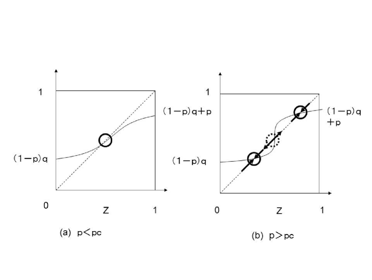
Figure 7: Solutions of self-consistent equation (66). (a) $p\leq p_{c}$ and (b) $p>p_{c}$. Below the critical point $p_{c}$, we can obtain one solution (a). We refer to this phase as the one-peak phase. In contrast, above the critical point, we obtain three solutions. Two of them are stable and one is unstable (b). We refer to this phase as the two-peaks phase.

For the network case, the self-consistent equations for the network case (37) and for the random graph case (19) are the same. Hence, we can obtain the mean-field approximation for the connectivity as (27).

References

- [1] Tarde G 1890 Les lois de l’imitation (Paris: Felix Alcan)
- [2] Milgram S, Bickman L, and Berkowitz L 1969 J. Per. Soc. Psyco. 13 79
- [3] Partridge B L 1982 Sci. Am. 245 90
- [4] Couzin I D, Krause J, James R, Ruxton G R, and Franks N R 2002 J. Theor. Biol. 218 1
- [5] Galam G 1990 Stat. Phys. 61 943
- [6] Cont R and Bouchaud J 2000 Macroecon. Dyn. 4 170
- [7] Eguíluz V and Zimmermann M 2000 Phys. Rev. Lett. 85 5659
- [8] Stauffer D 2001 Adv.Complex Syst. 4 19
- [9] Curty P and Marsili M 2006 JSTAT P03013
- [10] Araújo N A M, Andrade Jr. J S, and Herrmann H J 2010 PLOS ONE 5 e12446
- [11] Araripe L E, Costa Filho R N, Herrmann H J, Andrade Jr. J S 2006 Int. J. Mod. Phys. C17 1809
- [12] Castellano C, Fortunato S and Loreto V 2009 Rev. Mod. Phys. 81 591
- [13] Moreira A A , Paula D R, Costa Filho R N C and. Andrade Jr. J S 2006 Phys. Rev. E 73 065101(R)
- [14] Bikhchandani S, Hirshleifer D, and Welch I 1992 J. Polit. Econ. 100 992
- [15] Hisakado M and Mori S 2011 J. Phys. A 22 275204
- [16] Ito Y , Ogawa K and Sakakibara H 1974 July Stu Jour 11(3) 70 (in Japaneese)
- [17] Ito Y , Ogawa K and Sakakibara H 1974 October Stu Jour 11(4) 100 (in Japaneese)
- [18] Barabáshi A -L and Albert R 1999 Science 286 559
- [19] Bianconi G and Barabáshi A -L 2001 Euro Phys Lett54 436
- [20] Bianconi G and Barabáshi A -L 2001 Phy. Rev.Lett 865632
- [21] Hisakado M and Mori S 2010 J. Phys. A 43 3152 7
- [22] Watts D J and Dodds PS 2007 J. Consumer Research 34 441
- [23] Mori S, Hisakado M, and Takahashi T 2012 Phys. Rev. E 86 26109
- [24] Hisakado M and Mori S 2015 Physica A 417 63
- [25] Hisakado M, Kitsukawa K, and Mori S 2006 J. Phys. A 39 15365
- [26] Mori S and Hisakado M, Finite-size scaling analysis of binary stochastic processes and universality classes of information cascade phase transition, J. Phys. Soc. Jpn. 84 054001.
- [27] Mori S and Hisakado M, Correlation function for generalized Pólya urns: Finite-size scaling analysis ,arXiv:1501.00764
- [28] Watts D J and Strogatz S H 1998 Nature 393 440