Galaxy clusters in the SDSS Stripe 82
based on galaxy photometric redshifts

Abstract

Context. The discovery of new galaxy clusters is important for two reasons. First, clusters are interesting per se, since their detailed analysis allows us to understand how galaxies form and evolve in various environments and second, they play an important part in cosmology because their number as a function of redshift gives constraints on cosmological parameters.

Aims. We have searched for galaxy clusters in the Stripe 82 region of the Sloan Digital Sky Survey, and analysed various properties of the cluster galaxies.

Methods. Based on a recent photometric redshift (hereafter photo$-z$) galaxy catalogue, we built a cluster catalogue by applying the Adami & MAzure Cluster FInder (AMACFI). Extensive tests were made to fine-tune the AMACFI parameters and make the cluster detection as reliable as possible. The same method was applied to the Millennium simulation to estimate our detection efficiency and the approximate masses of the detected clusters. Considering all the cluster galaxies (i.e. within a 1 Mpc radius of the cluster to which they belong and with a photo$-z$ differing by less than $\pm 0.05$ from that of the cluster), we stacked clusters in various redshift bins to derive colour–magnitude diagrams and galaxy luminosity functions (GLFs). For each galaxy brighter than ${\rm M_{r}}<-19.0$, we computed the disk and spheroid components by applying SExtractor, and by stacking clusters we determined how the disk-to-spheroid flux ratio varies with cluster redshift and mass.

Results. We detected 3663 clusters in the redshift range $0.15\leq z\leq 0.70$, with estimated mean masses between $\sim 10^{13}$ and a few 10¹⁴ M_⊙. We cross-matched our catalogue of candidate clusters with various catalogues extracted from optical and/or X-ray data. The percentages of redetected clusters are at most 40% because in all cases we detect relatively massive clusters, while other authors detect less massive structures. By stacking the cluster galaxies in various redshift bins, we find a clear red sequence in the $(g^{\prime}-r^{\prime})$ versus $r^{\prime}$ colour-magnitude diagrams, and the GLFs are typical of clusters, though with a possible contamination from field galaxies. The morphological analysis of the cluster galaxies shows that the fraction of late-type to early-type galaxies shows an increase with redshift (particularly in 9$\sigma$ clusters) and a decrease with detection level, i.e. cluster mass.

Conclusions. From the properties of the cluster galaxies, the majority of the candidate clusters detected here seem to be real clusters with typical cluster properties.

1 Introduction

The cluster count technique (e.g. Gioia et al. 1990, Allen et al. 2011) is used to constrain cosmological parameters, and requires catalogues with large numbers of clusters at various redshifts, including high redshifts (z$\geq$1), and in extended fields of view (several tens of square degrees). This is why, with the advent of large cameras on 4m class telescopes, cluster searches at optical wavelengths have increased in number and redshift depth over these last ten years (see e.g. Durret et al. 2011b and references therein).

Several techniques have been applied to search for clusters, among which we particularly want to mention the ORCA (Overdense Red-sequence Cluster Algorithm) method, developed for the Panoramic Survey Telescope and Rapid Response System (Pan-STARRS) described in detail by Murphy et al. (2012) and applied by Geach et al. (2011, hereafter GMB; see below) to the same Stripe 82 region used in the present paper.

Other cluster searches were based on the red sequence in the colour magnitude diagram (Erben et al. 2009, Thanjavur et al. 2009). Among other techniques used to search for clusters in large imaging surveys, a matched filter detection algorithm was applied to the Canada France Hawaii Telescope Legacy Survey (CFHTLS) Deep fields (Olsen et al. 2007, 2008, Grove et al. 2009, Milkeraitis et al. 2010). The combination of optical and infrared imaging surveys has recently led to the discovery of many high redshift ($z>1.1$) groups and clusters (Bielby et al. 2010). Lensing techniques were employed to detect massive structures (i.e. with masses larger than $10^{13}$ M_⊙) in the CFHTLS (e.g. Cabanac et al. 2007, Gavazzi $\&$ Soucail 2007, Bergé et al. 2008, Limousin et al. 2009). More recently, weak lensing mass measurements were made for clusters in part of the CFHTLS Wide survey (Shan et al. 2012). A Bayesian cluster finder has been applied to detect galaxy clusters in the CFHTLS by Ascaso et al. (2012) and in the Deep Lens Survey by Ascaso et al. (2014). Van Breukelen & Clewley (2009) developed yet another algorithm, named 2TecX, to search for high redshift clusters in optical/infrared imaging surveys. This method is based on photometric redshifts (hereafter photo$-z$s) estimated from the full redshift probability function and on the identification of cluster candidates by cross-checking two different selection techniques (adaptations of the Voronoi tessellations and of the friends-of-friends method). The most recent technique, redMapper, has been developed by Rykoff et al. (2014) and applied to the SDSS DR8.

Geach et al. (2011) have searched for clusters in Stripe 82, a region of the Sloan Digital Sky Survey (SDSS) covering a surface of 270 deg² across the celestial equator in the Southern Galactic Cap ($-50^{\circ}<\alpha<59^{\circ}$, $|\delta|\leq 1.25^{\circ}$). They found 4098 clusters up to redshift $z\sim 0.6$ with a median redshift z=0.32. To do this, they applied an algorithm that searches for statistically significant overdensities of galaxies in a Voronoi tessellation of the projected sky. They define a cluster as having at least five galaxy members, so we expect them to detect a higher number of clusters than that obtained with our method. Geach et al. (2011) published a full cluster catalogue, allowing us to compare our results directly to theirs.

We have developed a method to search for clusters in large multiband imaging surveys: AMACFI (Adami & MAzure Cluster FInder, Adami & Mazure 1999). We have applied it to the CFHTLS Deep and Wide fields (Mazure et al. 2007, Adami et al. 2010, Durret et al. 2011b, hereafter M07, A10, and D11, respectively). We have recently confirmed spectroscopically two clusters at $z=0.61$ and $z=0.74$ detected in the CFHTLS Deep 3 field (Adami et al. 2015a), and a third one at $z=0.53$ (Adami et al. 2015b), and this gives us yet more confidence in our method. We have also applied AMACFI to the Stripe 82 data and present our results below.

We must keep in mind that all these cluster searches produce lists of cluster candidates. It is therefore important to see whether different methods lead to the same cluster detections, and we will therefore compare our list of cluster candidates with other available cluster catalogues.

The paper is organized as follows. The data and method used to search for clusters is briefly summarized in Section 2. Results on cluster candidates are described in Section 3: catalogue and redshift distribution. In Section 4 we compare our cluster candidates to those found with other detection algorithms. By stacking clusters in redshift bins of 0.1, we obtained colour-magnitude diagrams and galaxy luminosity functions, and discuss these results in Section 5. We then compute in Section 6 the fraction of early- to late-type galaxies in stacked clusters as a function of redshift and of cluster mass. A brief discussion and conclusions are given in Section 7.

In this paper we assume H₀ = 70 km s^-1 Mpc^-1, $\Omega_{m}$=0.3, $\Omega_{\Lambda}$=0.7.

2 Data and method

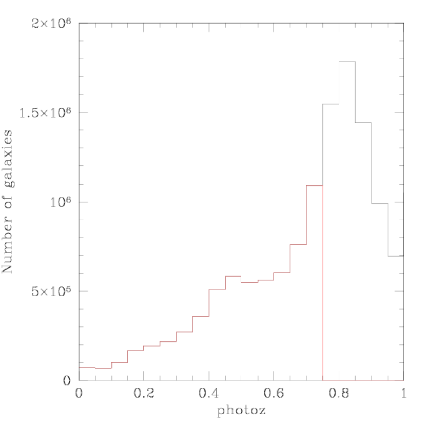
Figure 1: Photometric redshift histogram for the initial sample of 13,621,717 objects (black) and for the selected sample of 6,110,921 objects with z${}_{phot}\leq 0.75$ (red).

The SDSS has obtained many scans in the so-called Stripe 82 (hereafter S82) field, defined by right ascension approximately in the range 310${}^{\circ}-59^{\circ}$ and declination $|\delta|\leq 1.25^{\circ}$ (J2000). Five photometric bands are available: $u^{\prime},\ g^{\prime},\ r^{\prime},\ i^{\prime}$, and $z^{\prime}$. These repeated observations have been averaged to produce deeper and more accurate photometry than the nominal 2% single-scan photometric accuracy (Ivezić et al. 2004).

2.1 Stripe 82 catalogues

We started with the Msplit catalogue of 13,621,717 objects available in the SDSS database. For each object this catalogue contains the SDSS identification (19 digit number), right ascension, declination, photo$-z$, and error on the photo$-z$ made by Reis et al. (2012), and is limited in magnitude to $r^{\prime}<24.5$. The photo$-z$ histogram of these 13,621,717 objects is shown in Fig. 1. To avoid incompleteness (which becomes apparent in Fig. 1 for z${}_{phot}\sim 0.8$), we cut this catalogue at z${}_{phot}\leq 0.75$ and were then left with 6,110,921 objects. This photo$-z$ catalogue was used to detect cluster candidates.

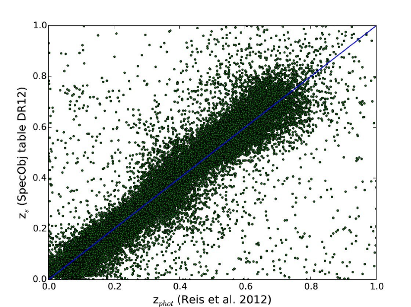
Figure 2: Spectroscopic redshifts in the S82 region taken from SDSS DR12 versus photometric redshifts from Reis et al. (2012) for 105,613 galaxies. The blue line shows the diagonal of the square.

As a check to the quality of the Reis photo$-z$ catalogue, we cross-correlated it with the SDSS spectroscopic catalogue, SpecObj table of the recent data release DR12. The result is shown in Fig. 2 for 105,613 galaxies. For the difference $|z_{p,{\rm Reis}}-z_{s}|$ between the Reis photo$-z$s $z_{p,{\rm Reis}}$ and the spectroscopic redshifts $z_{s}$, the mean value is 0.027, the median is 0.016, and the standard deviation is 0.047. As a comparison, we made the same correlation between the DR12 photo$-z$s extracted from the Photoz table and the spectroscopic redshifts $|z_{p,{\rm DR12}}-z_{s}|$ and found a mean value of 0.038, a median of 0.023, and a standard deviation of 0.053. This confirms that the Reis photo$-z$ catalogue is better than the general Photoz DR12 catalogue, and we will therefore use the Reis catalogue for our analysis. The fact that there are very few spectroscopic redshifts above $z\sim 0.8$ to calibrate the photo$-z$s justifies our cut at $z_{phot}=0.75$.

We also retrieved the dereddened magnitude catalogue of 8,485,885 objects (Annis et al. 2014) which we later cross-correlated with the photo$-z$ catalogue to obtain a complete catalogue of 4,999,968 galaxies that was fed into the Le Phare software (Arnouts et al. 1999, Ilbert et al. 2006) to compute the absolute magnitudes that we will exploit further in the paper.

We first considered the curves shown in Fig. 8 of Annis et al. (2014) to estimate the 90% completeness limit of our magnitude catalogue. These give the following approximate values: $u^{\prime}_{lim}$=23.1, $g^{\prime}_{lim}$=22.8, $r^{\prime}_{lim}$=22.4, $i^{\prime}_{lim}$=22.1, and $z^{\prime}_{lim}$=20.4. However, when drawing the magnitude histograms in the five photometric bands (see Fig. 16) and superimposing these limits (marked as dotted vertical lines), we found that although in the $u^{\prime}$ and $g^{\prime}$ bands the Annis limits seemed acceptable (i.e. brighter than the magnitude when incompleteness becomes obvious), in the $r^{\prime}$ and $i^{\prime}$ bands these limits were obviously too faint while in the $z^{\prime}$ band the limit was too bright. We therefore take the following (rather conservative) 90% completeness limits: $u^{\prime}_{lim}$=23.0, $g^{\prime}_{lim}$=22.8, $r^{\prime}_{lim}$=22.1, $i^{\prime}_{lim}$=21.5, and $z^{\prime}_{lim}$=21.2 (marked as full vertical lines in Fig.16).

2.2 Method for cluster detection

2.2.1 Overall description of the method

We applied to this photo$-z$ catalogue the same treatment as in M07, A10, and D11, where a full description is given. This method has also been applied by A10 to the Millennium simulation (Springel et al. 2005) to assess the quality of the detections and to obtain a rough estimate of the relation between the cluster masses and the significance level at which clusters were detected. We have done the same for the S82 data, as described below.

We first divided the photo$-z$ catalogue in slices of 0.1 in redshift, each slice overlapping the previous one by 0.05 (i.e. the first slice covers redshifts 0.1 to 0.2, the second 0.15 to 0.25, etc. and the last slice is 0.65–0.75). As discussed by A10, the 0.1 redshift width of the studied slices is the best compromise between the redshift resolution and the possible dilution of the density signal due to typical photometric redshift uncertainties. Then, to make the data manageable (in ram-active CPU memory), each subcatalogue was then divided into slices of 1.1 deg in right ascension, with an overlap of 0.1 deg between slices. No cut was made in declination.

We built galaxy density maps for each redshift slice, based on the adaptative kernel technique described in M07, with a pixel size (originally taken to be 1 arcmin) that will be discussed below and 100 bootstrap resamplings of the maps to estimate the background level correctly.

We then detected structures in these density maps with the SExtractor software (Bertin & Arnouts 1996) in the different redshift bins at various significance levels: 3$\sigma$, 4$\sigma$, 5$\sigma$, 6$\sigma$, and 9$\sigma$ (as defined by SExtractor).

The structures were then assembled in larger structures (called $detections$ in the following) using a minimal spanning tree friends-of-friends algorithm (see Adami & Mazure 1999). Two $detections$ with centres distant by less than 2 arcmin (twice the pixel size defined originally) were merged into a single one which was assigned the redshift of the $detection$ having the highest S/N. We did not merge $detections$ within 2 arcmin into a single one if their photometric redshifts differed by more than 0.09 to avoid losing clusters that could be almost aligned along the line of sight but located at very different redshifts. With this separation limit (hereafter called the separation parameter), the typical uncertainty on cluster positions is therefore about 2 arcmin. This respectively corresponds to 310 kpc and 860 kpc at $z=0.15$, the lowest redshift, and $z=0.7$, the highest redshift in our cluster sample. We also briefly discuss below the influence of the choice of this separation limit on the final cluster catalogue.

2.2.2 Choice of pixel size for the density maps and of the separation parameter

We initially built galaxy density maps for each redshift slice, with a pixel size of $1.002\times 1.002$ arcmin². With this pixel size we obtained a cluster catalogue containing 956 clusters in the redshift range of 0.15–0.7. Since S82 covers an area of 270 deg², the spatial density of this catalogue is 956/270 = 3.54 clusters deg^-2, while if we consider the clusters detected in the CFHTLS–Wide 1, Wide 2, Wide 3, and Wide 4 (D11) in the same redshift range ($0.15\leq z\leq 0.70$), we find respective densities of 17.0, 15.9, 14.8, and 16.6 clusters deg^-2, using a pixel size of 0.54 arcmin and a separation parameter of 3 arcmin. When the search for clusters in the CFHTLS was made, the separation parameter was still an angle, while in the minimal spanning tree code we now implement a separation in Mpc, which is more physical. So our detection level in S82 was smaller than that of the CFHTLS–Wide by a factor between 4.2 and 4.8. A first explanation could be that the S82 catalogue is shallower than that of the CFHTLS, and does not reach similar redshifts and/or magnitudes. However, if we compare the galaxy photo$-z$ histogram of the S82 to that of the CFHTLS Wide survey (Fig. 2 in D11, black line), we can see that the S82 histogram starts decreasing for z$>$0.85, while the CFHTLS–Wide starts decreasing for z$>$0.90, so the photo$-z$ completeness limit of S82 is lower than that of the CFHTLS–Wide only by $\sim 0.05$. If we compare the magnitude completeness limits of the two surveys, the S82 90% completeness limit is reached for r$\sim 22.1$ according to Annis et al. (2014). In the CFHTLS–Wide, incompleteness begins to show for $i^{\prime}\sim 23.5$, which corresponds to $r^{\prime}$ between 22.5 and 23 (for an elliptical galaxy at redshift 0.2 or 0.5, respectively), showing that the S82 catalogue is shallower that the CFHTLS–Wide only by approximately half a magnitude. So the discrepancy by a factor of 4 between the density of clusters detected with AMACFI in the two surveys seems too large to be explained only by their difference in depth. This led us to question our method and to make several tests, first on the pixel size chosen to compute the density maps on which our cluster detection is based, and second on the separation parameter.

Since the CPU time necessary to compute density maps increases dramatically as the pixel size decreases (and hence the number of pixels increases), we made the following tests on a subregion of S82 covering $1<$RA$<10$ deg, with the full declination range $|\delta|\leq 1.25^{\circ}$. We considered pixel sizes of $30\times 30$ arcsec², $15\times 15$ arcsec², and $10\times 10$ arcsec². As the pixel size decreases, the number of structures detected increases, so the completeness of the cluster catalogue increases. However, we must be careful not to start detecting very small structures that cannot be clusters, because in this case the purity of the cluster catalogue will decrease.

As mentioned above, we took a separation parameter of 2 Mpc. Since the separation parameter could have an influence on the number of candidate clusters detected, we made tests with separation parameters of 1 Mpc, 2 Mpc, and 3 Mpc, and the results are given below.

We also tested how the quality of the photo$-z$s could influence the numbers of candidate clusters detected by applying two different selections. First, we considered only the galaxies with an error $\delta_{zp}\leq 0.1$ on their photo$-z$. Such a cut reduces the number of galaxies with photo$-z\leq 0.75$ from 6,110,921 to 2,458,235, and therefore excludes 59.8% of the galaxies. Second, we considered only the galaxies with a relative error smaller than 50%: $\delta_{zp}/z_{p}\leq 0.5$. In this case, the total number of galaxies drops from 6,110,921 to 4,469,271, and thus we exclude 26.9% of the galaxies.

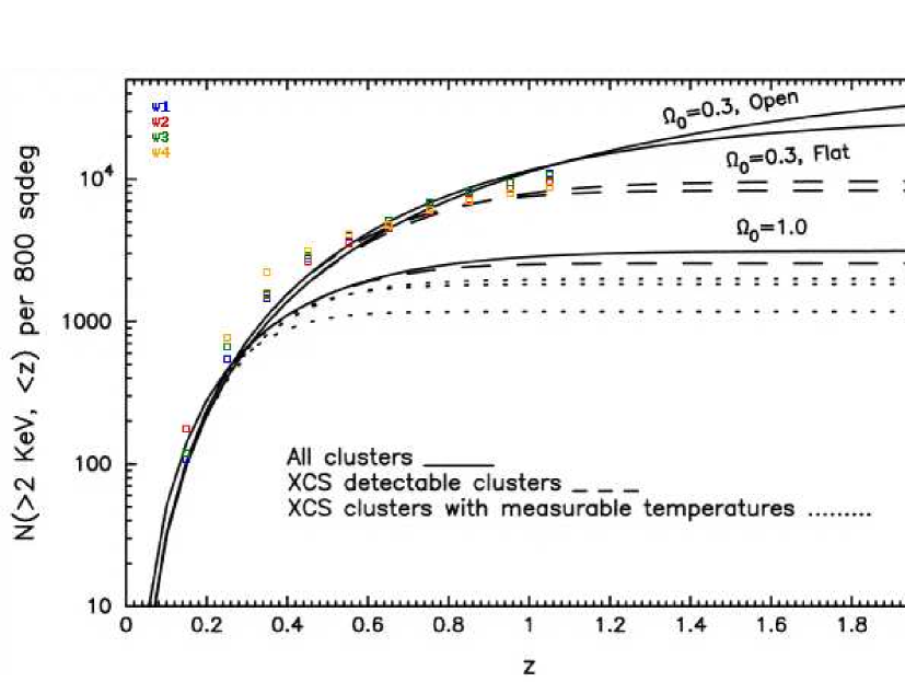
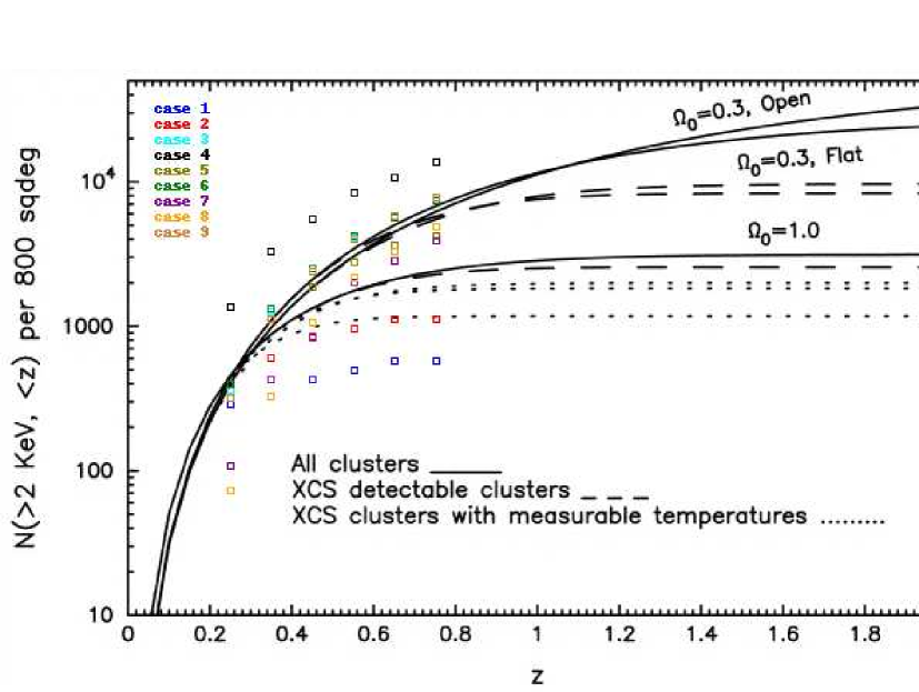
Figure 3: Cumulative number of clusters hotter than 2 keV expected in a region of 800 deg² for different cosmologies as a function of redshift, taken from Romer et al. (2001), Fig. 5. The numbers of clusters in the four CFHTLS–Wide fields are shown in the top figure, and the numbers detected in Stripe 82 for the various cases described in Table 1 (see text) are plotted in the bottom figure. Only clusters detected at a 4$\sigma$ level and above are taken into account.

In order to have an objective criterium for the choice of the cluster detection parameters, we considered the plots showing the cumulative number of clusters hotter than 2 keV expected in a region of 800 deg² for different cosmologies as a function of redshift, taken from Romer et al. (2001), Fig. 5b. The mass-temperature relation of Xu et al. (2001) implies that kT$>$2 keV corresponds to clusters of masses M${}_{r200}>(1.2-1.6)\times 10^{14}$ M_⊙. As a first test, we overplotted on these curves the densities of clusters detected by D11 in the four CFHTLS Wide fields. We found a very good agreement between our cluster densities and the Romer curves for $\Omega_{0}=0.3$ when considering the clusters detected at 4$\sigma$ and above, as illustrated in Fig. 3 (top). We then overplotted on the same curves the densities of clusters detected at a 4$\sigma$ level in a subregion of S82 defined by $1<$RA$<10$ deg and $|\delta|\leq 1.25^{\circ}$ for the nine cases summarized in Table 1.

Table 1: Cases considered in the various tests on cluster detection parameters. The columns are: (1) running number of test; (2) pixel size chosen to compute the density maps; (3) separation, that is the minimum value above which two detected structures are considered to be different if they differ by more than 0.09 in redshift; (4) cut depending on the photometric redshift uncertainty when applicable.

Case	pixel size	separation	cut on $z_{p}$
	(arcsec$\times$ arcsec)	(Mpc)
1	60$\times$60	2	$-$
2	30$\times$30	2	$-$
3	10$\times$10	2	$-$
4	10$\times$10	1	$-$
5	15$\times$15	2	$-$
6	10$\times$10	2	$\Delta z_{p}/z_{p}\leq 0.5$
7	10$\times$10	3	$\Delta z_{p}/z_{p}\leq 0.5$
8	10$\times$10	3	$\Delta z_{p}\leq 0.1$
9	10$\times$10	3	$-$

In Table 1, for each case we give the pixel size chosen to compute the density maps and the “separation”, that is the minimum value above which two detected structures are considered to be different if they differ by more than 0.09 in redshift. In some cases we have also applied a cut based on the error on the photo$-z$.

We now compare the numbers of clusters detected at a 4$\sigma$ level and higher in Stripe 82 to the Romer et al. (2001) curves, as shown in Fig. 3 (bottom). First, we can see that our original choice of parameters (case 1) leads to a number of clusters that is much too small. Pixel sizes of $30\times 30$ arcsec² (case 2) and $15\times 15$ arcsec² (case 5) also lead to too few clusters. If we take a separation equal to 1 Mpc or 3 Mpc (cases 4 and 7, respectively), the numbers of clusters fall clearly above and below the Romer curve, so we decided to keep a separation of 2 Mpc. The number of clusters detected in case 8 is also much too small. The best match with the Romer et al. curves is obtained for cases 3, 6, and 9. In order to keep our sample as similar as possible to the cluster sample extracted in the CFHTLS-W, we chose to make the cluster detection on the full catalogue (limited to $z_{p}\leq 0.75,$ but with no condition on the photo$-z$ error) with a pixel size of $10\times 10$ arcsec² and a separation of 2 Mpc (case 3).

In this way we obtained a final catalogue of 3663 candidate clusters detected at a significance level from 3$\sigma$ to 9$\sigma$. This catalogue– including for each cluster the coordinates, photo$-z$, detection level and number of cluster galaxies– will be available at the VizieR interface of the Simbad database.

3 Cluster catalogue

3.1 Significance level and spatial distribution of the candidate clusters

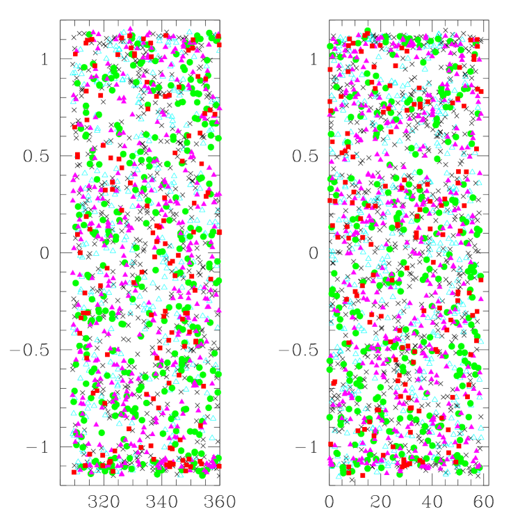
Figure 4: Projected spatial distribution of the 3663 candidate clusters, colour coded as follows: red squares: S/N=$9\sigma$, magenta filled triangles:S/N$=6\sigma$, green filled circles: S/N$=5\sigma$, cyan empty triangles: S/N$=4\sigma$, black crosses: S/N$=3\sigma$.

In the catalogue of 3663 cluster candidates, the numbers of clusters detected at the various significance levels of 3$\sigma$, 4$\sigma$, 5$\sigma$, 6$\sigma$, and 9$\sigma$ are: 1133, 792, 623, 820, and 295, respectively. In Sections 5 and 6 we concentrate on the properties of the 2530 clusters detected at $4\sigma$ and above to limit our analysis to the objects that are the most likely to be real clusters.

The projected spatial distribution of all the detected clusters is shown in Fig. 4 with different symbols for the various significance levels. We can see concentrations of candidate clusters at the edges in declination, for $|\delta|\sim 1.1-1.2$, which are most probably spurious detections. We keep these objects in our final catalogue for the sake of completeness, but we note this shortcoming.

3.2 Redshift distribution of the candidate clusters

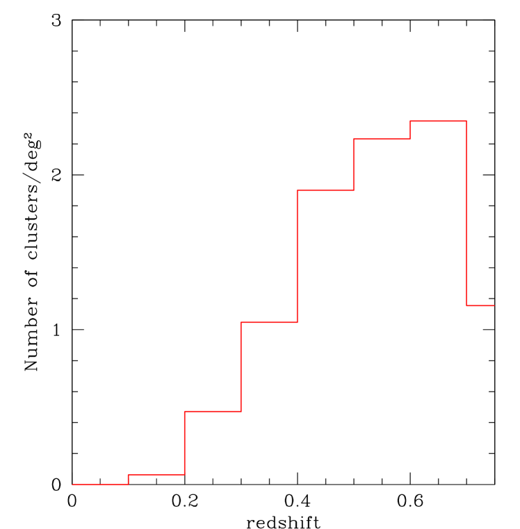
Figure 5: Histogram of the surface density of cluster candidates in S82 as a function of photometric redshift.

The photometric redshift distribution of the 3663 candidate clusters detected in S82 in the redshift range 0.15–0.7 (divided by 270 deg² to obtain a surface density directly comparable to those found in the literature) is shown in Fig. 5. This photo$-z$ distribution has a mean value of 0.51 and a median of 0.53, with dispersions of 0.15 around these values. The median redshift of our clusters is notably higher than the median redshift z=0.32 found by Geach et al. (2011) for their sample of 4098 clusters, and the comparison between both samples will be made in Section 4.

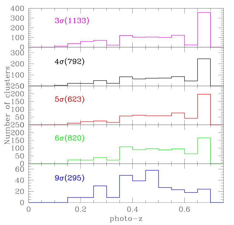
Figure 6: Photometric redshift histograms of the 3663 candidate clusters detected in S82 for various detection significance levels (indicated in each plot, together with the corresponding number of clusters in parentheses). For clarity, the scale of the y-axis is not the same for each plot.

The photo$-z$ histograms for clusters detected at different significance levels are shown in Fig. 6.

3.3 Cluster masses

By applying the same detection method to the Millennium simulation, we have shown (see A10, Table 2) that there is a rough correspondence between the cluster detection level and its mass. We have redone the same exercise, selecting data from the Millennium simulation and adapting them to the conditions of the S82 data analysed here, in terms of photometric redshift precision and photometric catalogue depth.

Table 2: Percentages of Millennium haloes detected with our method as a function of lower mass cutoff. The columns are: (1) halo mass in units of $10^{12}$ M_⊙; (2)–(7) percentages of redetected haloes in the following redshift intervals: $z1:z\leq 0.2$, $z2:0.2<z\leq 0.3$, $z3:0.3<z\leq 0.4$, $z4:0.4<z\leq 0.5$, $z5:0.5<z\leq 0.6$, and $z6:0.6<z\leq 0.8$.

${\rm M_{halo}}$	$z1$	$z2$	$z3$	$z4$	$z5$	$z6$
250	-	100	66	33	20	0
65	66	68	54	10	5	0
20	75	68	59	2	1	0
7.5	76	63	67	2	1	0
3.0	67	64	59	1	1	0

We ran AMACFI on this catalogue, exactly in the same way as for the S82 galaxy catalogue, and detected 30 structures. The percentages of detected haloes are given in Table 2 for five classes with masses ranging from $3.0\times 10^{12}$ M_⊙ to $2.5\times 10^{14}$ M_⊙ in six redshift bins: $z\leq 0.2$, $0.2<z\leq 0.3$, $0.3<z\leq 0.4$, $0.4<z\leq 0.5$, $0.5<z\leq 0.6$, and $0.6<z\leq 0.8$.

We can see that for all the haloes the percentage of detections is larger than about 60% up to $z\sim 0.4$. In the next redshift bin, this percentage drops to 33% and 10% for the two most massive haloes and becomes extremely low for the three least massive haloes. The corresponding orders of magnitude for the masses are that clusters detected at 3$\sigma$ and 4$\sigma$ have masses in the approximate range [$10^{13}-10^{14}$ M_⊙], while clusters detected at 6$\sigma$ have masses larger than $10^{14}$ M_⊙. As in A10, because the Millennium simulation only covers an area corresponding to 1 deg², it includes no cluster corresponding to a 9$\sigma$ detection in our study, so we cannot estimate the typical mass of the clusters detected at a 9$\sigma$ level; all we can say is that these clusters must have masses larger than $10^{14}$ M_⊙.

By varying the detection parameters used in SExtractor, we estimate that the errors on these halo masses are of the order of 5%.

3.4 Cluster spatial density

We found 3663 clusters in a region of about 270 deg² in the redshift range 0.15–0.70, which gives a detection rate of about 13.6 clusters per square degree. Geach et al. (2011) detected 3896 clusters in the same redshift range, corresponding to about 14.4 clusters per square degree, a detection rate 1.06 times higher than ours. This small difference is most probably due to the fact that they call “a cluster” any structure with five galaxies or more. The application of our cluster detection method to the Millennium simulation shows that the minimum mass of a $3\sigma$ detected cluster is $\sim 10^{13}$ M_⊙, and we therefore do not detect less massive structures.

We can also compare the cluster density that we find in S82 with that found in the four CFHTLS Wide fields. In these fields, we have detected 4061 candidate clusters at 3$\sigma$ and above, corresponding to between 21 and 28 clusters per square degree (depending on the field considered), reaching redshift 1.15 (see D11). The corresponding cluster densities for $0.15\leq z\leq 0.7$ are between 14.8 and 17.0 clusters per square degree. The cluster density detected in S82 is therefore of the same order of magnitude as in the CFHTLS, as seen from the comparison of Fig. 5 in the present paper with Fig. 7 (bottom) in D11.

3.5 Number and magnitude distributions of the cluster galaxies

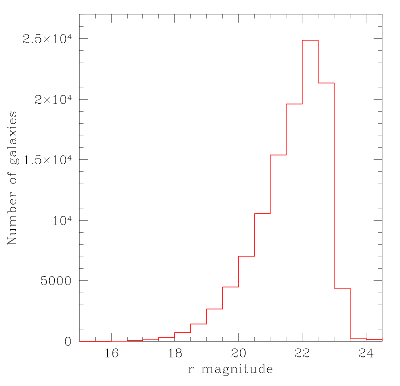
Figure 7: Magnitude histogram of the cluster galaxies in the r band.

We define cluster galaxies as the galaxies located within a circle of 1 Mpc radius around each cluster and within $\pm 0.05$ of the redshift of the cluster to which they belong. The magnitude histogram of the 113,411 cluster galaxies in the r band is shown in Fig. 7.

4 Comparison with optically and X-ray detected clusters in S82

Table 3: Common systems in our cluster catalogue and in other optically and X-ray selected cluster catalogues within a search radius of 2 Mpc. The percentages of recovered systems in the published catalogues are given in parentheses.

Catalogue	$z_{phot}$ range	NClG	NClG,match	NClG,match
			$\Delta z<0.05$	$\Delta z<0.1$
GMB	$0.15\leq z_{p}\leq 0.70$	3896	472 (12%)	838 (22%)
WHL12	$0.15\leq z_{p}\leq 0.70$	2901	538 (19%)	838 (29%)
RedMaPPer	$0.15\leq z_{p}\leq 0.55$	665	188 (28%)	268 (40%)
XCS-DR1	$0.15\leq z_{p}\leq 0.70$	28	5 (18%)	7 (25%)
XMM/SDSS	$0.15\leq z_{p}\leq 0.68$	30	5 (17%)	6 (20%)

We have cross-correlated our catalogue of candidate clusters with several catalogues extracted from optical and/or X-ray data: GMB, WHL12 (Wen et al. 2012), RedMaPPer (Rykoff et al. 2014), XCS-DR1 (Mehrtens et al. 2012), and XMM/SDSS (Takey et al. 2013, 2014). The matching criteria were a linear separation smaller than 2 Mpc and a redshift difference smaller than 0.05 or 0.1 (see e.g. Hao et al. 2010). The numbers of clusters in common are given in Table 3.

Geach et al. (2011) detected 4098 clusters in the S82 region, but with a different definition, since they consider that a cluster begins with five galaxies. The number of recovered clusters from the GMB catalogue is 22%, a rather low number. This can be explained by the fact that 73% of the GMB clusters have less than ten members, while the clusters in our sample with the lowest richness have several tens of galaxies.

The rather low number of recovered clusters from the WHL12 catalogue (29%) can be explained in the same way: 30% of the clusters in WHL12 have 10 members or fewer (in the $r^{\prime}_{200}$ radius), and 86% have 20 members or fewer, so WHL12 detect clusters that are mostly less massive than ours.

In the RedMaPPer catalogue, Ryckoff et al. (2014) give two parameters ($\Lambda$ and S) that can be used to determine the number of cluster galaxies $N=\Lambda/S$, where $N$ is in the range 20–203. About 64% of their clusters have $N<30$ and their cluster masses are M${}_{r200}\geq 10^{14}$ M_⊙. We recover 40% of their clusters.

Since the detection of our candidate clusters as diffuse X-ray sources would be an obvious way to confirm that they are real clusters, we also correlate our detections with the XCS-DR1 catalogue (Mehrtens et al. 2012). This X-ray catalogue has 41 clusters in the S82 region (as defined in Section 1), among which 28 are in the same redshift range as ours. Our matching percentage is 25%.

A similar survey to the XCS is the 2XMMi/SDSS galaxy cluster survey (Takey et al. 2011, 2013, 2014) that provided 35 clusters in the S82 region. Of these, 30 clusters are almost in the same redshift range [0.15–0.68] as our S82 cluster candidates. About 70% of these clusters have masses M${}_{500}<10^{14}$ M_⊙. With our cross-matching criteria, we have recovered 20% of the 2XMMi/SDSS clusters that are in the S82 region and in the redshift range 0.15–0.68.

Other observational biases can, however, be present. X-ray serendipitous surveys such as the XCS and 2XMMi/SDSS make use of existing XMM observations for which the main targets are most of the time not the detected clusters. For example, bright stars or large nearby galaxies can have been targeted, and this would obviously result in a large masking percentage of the S82 optical data, potentially preventing us from detecting the X-ray extended structure as a galaxy concentration. In addition, these serendipitous surveys of clusters avoided the clusters (usually the massive ones) that were targets of pointed XMM-Newton observations. All these observational biases reduce the recovered fraction of the X-ray selected clusters. It is worth performing a detailed comparison of X-ray clusters and our S82 clusters similar to the X-CLASS-redMaPPer galaxy cluster comparison (Sadibekova et al. 2014). We therefore plan in the near future to make this detailed comparison.

5 Properties of stacked clusters

In this section we will limit our analysis to the 1738 clusters detected at 5$\sigma$ and above, and to galaxies within a radius of 1 Mpc of a cluster and with a photo$-z$ within $\pm 0.05$ of that of the corresponding cluster for two reasons: first, to avoid having too much contamination by galaxies that do not belong to the clusters, and second to derive galaxy luminosity functions (GLFs) in redshift bins of width 0.1 that do not overlap.

5.1 Colour-magnitude diagrams

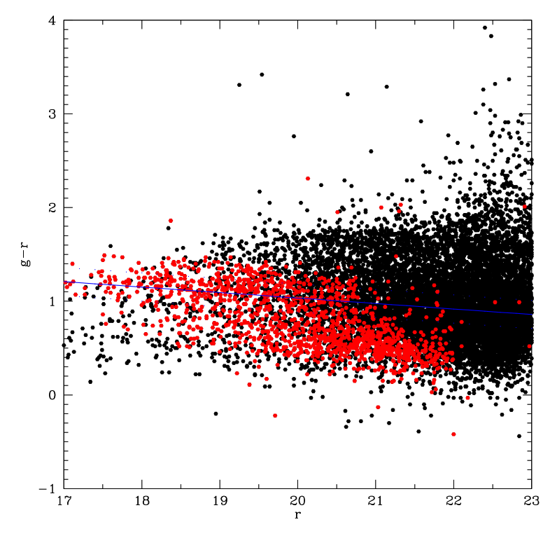
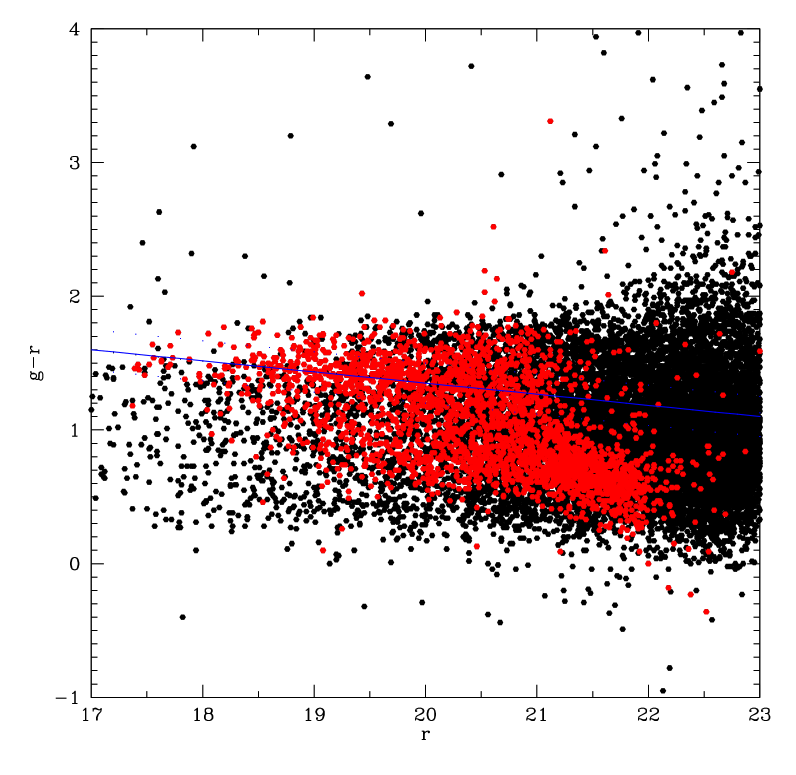
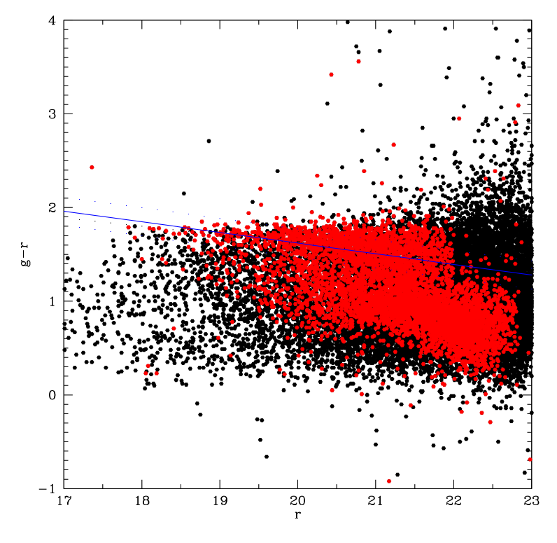
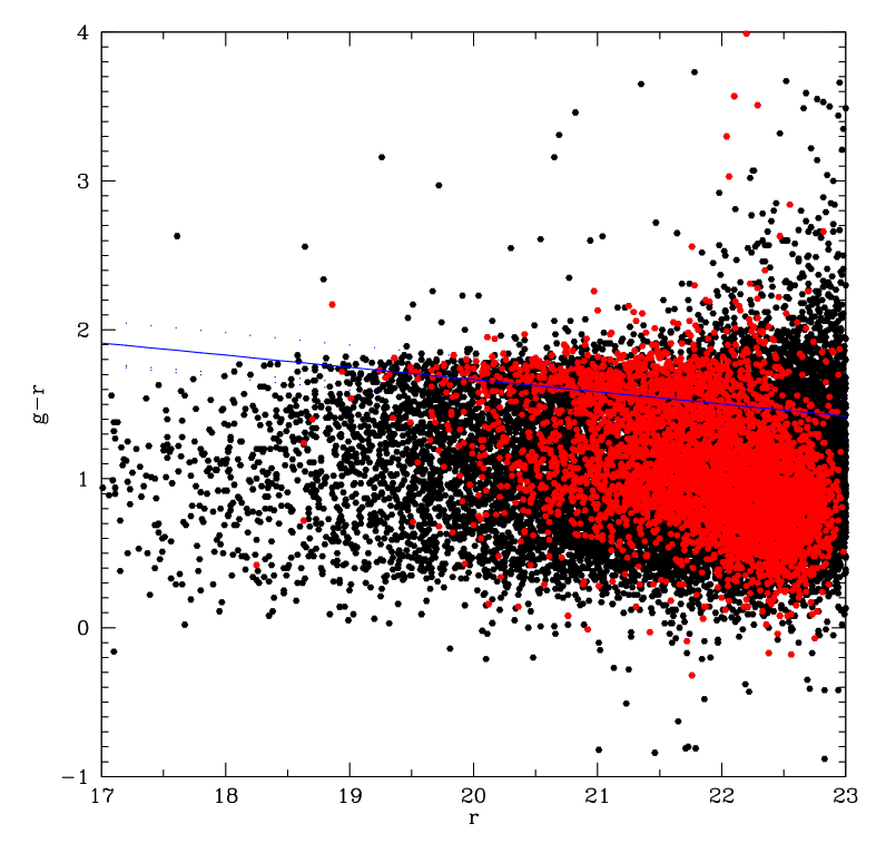
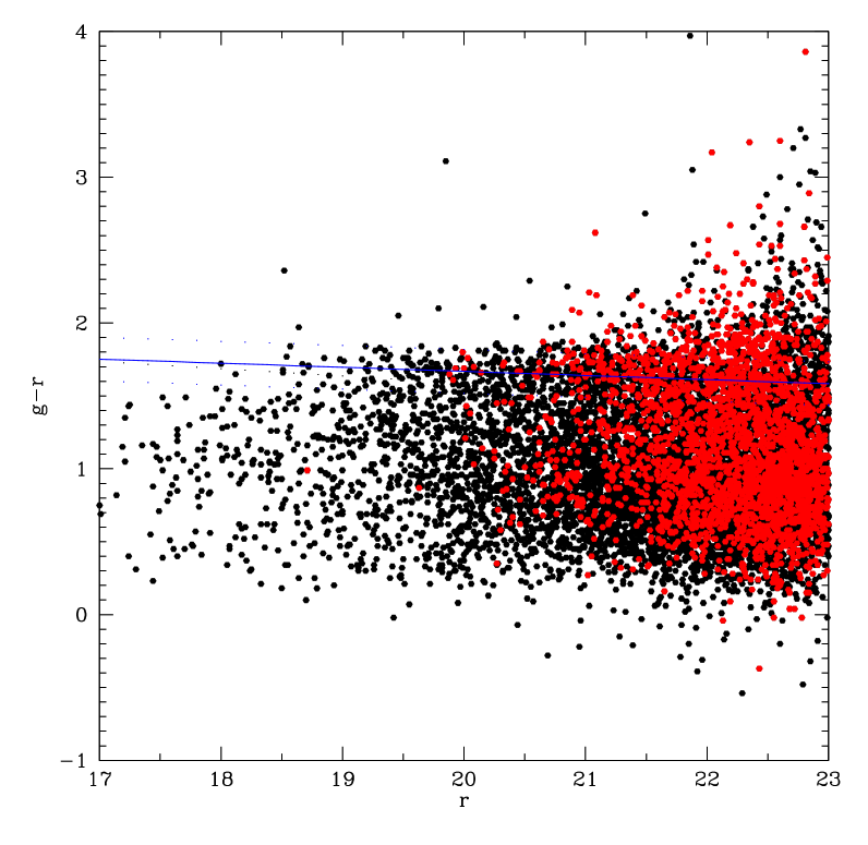
Figure 8: Colour-magnitude diagrams ($(g-r)$ versus $r^{\prime}$) stacked in the five redshift bins (from left to right: $0.15<z<0.25$, $0.25<z<0.35$, $0.35<z<0.45$, $0.45<z<0.55$, $0.55<z<0.65$) before background subtraction (see text). The black points show all the galaxies within a radius of 1 Mpc of a cluster, and the red points correspond to the galaxies with a photometric redshift within $\pm 0.05$ of that of the cluster to which they belong. The solid blue line shows the best fit.

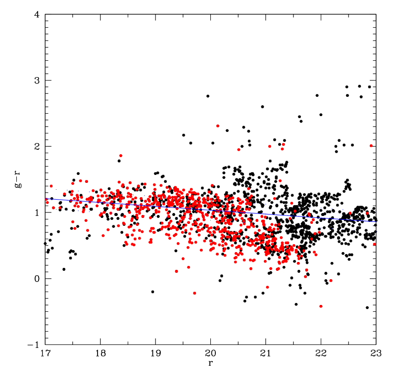
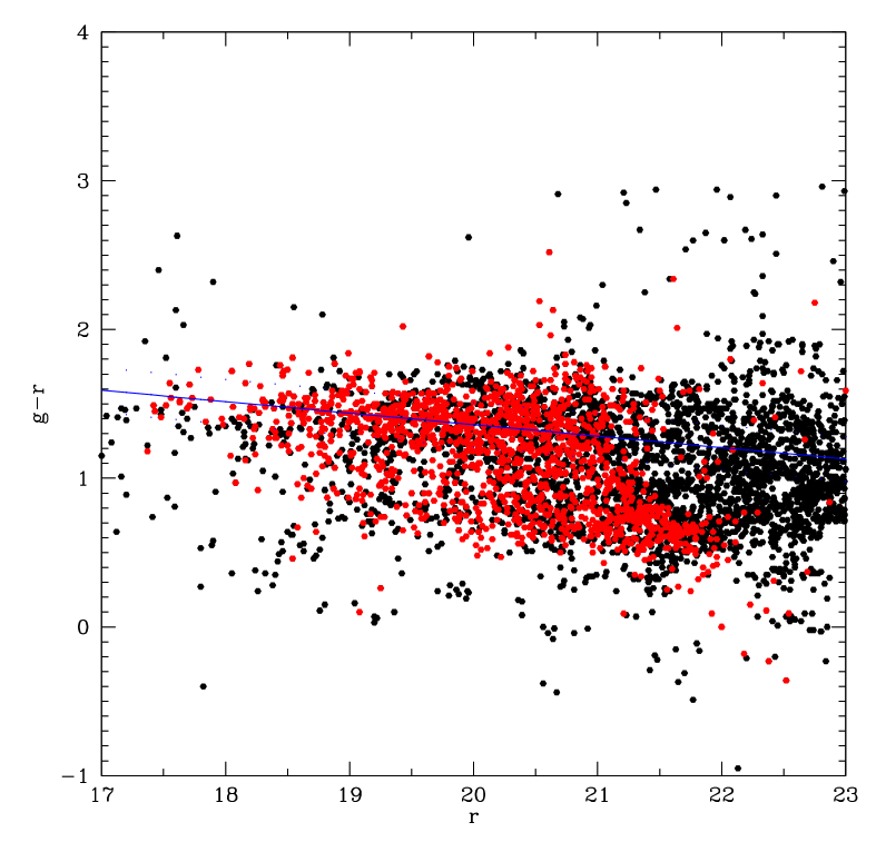
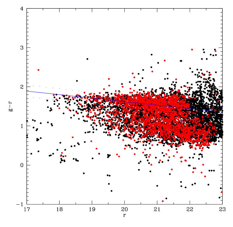
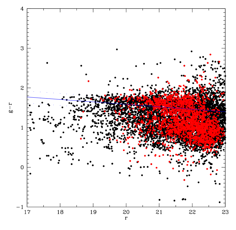
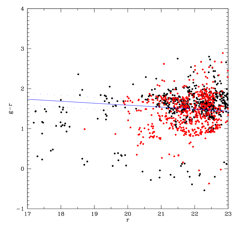
Figure 9: Same as Fig. 8 after background subtraction.

We first derive colour-magnitude diagrams by stacking galaxies in photometric redshift bins. The red sequence is apparent in all colour-magnitude diagrams, but the $(g-r)$ versus $r^{\prime}$ colour-magnitude diagram is the one that shows the smallest dispersion, and so we use it to select cluster galaxies and build GLFs. We show these diagrams in five redshift bins in Figs. 8 and 9, respectively, before and after background correction (see Section 5.2.2 for explanations on the method used to subtract the background contribution).

The fact that we detect a red sequence shows that we have selected galaxies with similar star formation histories that belong to well-assembled structures, and therefore that our candidate clusters are mostly old galaxy structures. As seen in these figures, the red sequence defined by the cluster galaxies is in good agreement with the predictions of the Bruzual & Charlot (2003) model.

5.2 Galaxy luminosity functions

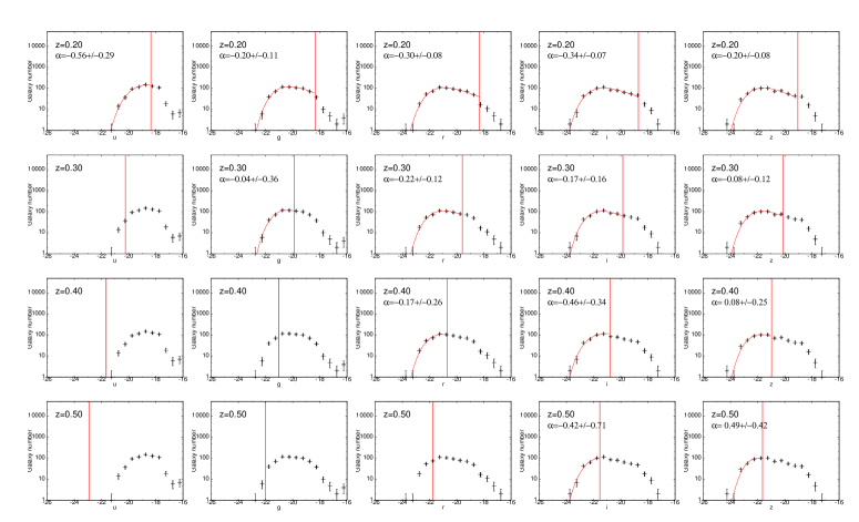
Figure 10: GLFs in the u, g, r, i and z bands (from left to right). Black crosses are the stacked GLFs with no surface normalization. The red curves are the best Schechter fits corresponding to the black crosses. The vertical red lines indicate the 90% completeness limits. Only galaxies brighter than the 90% completeness limit are taken into account for the fits. The plots for which no Schechter parameters are given in Table 4 are only shown for completeness, but will not be taken into account in the discussion.

5.2.1 Computing absolute magnitudes and 90% completeness limits

In order to be able to stack the cluster GLFs it was necessary to compute absolute magnitudes for all the galaxies. For this, we applied the Le Phare software as described in Section 2.1, with photo$-z$s fixed to the SDSS values.

Since the GLF parameters can strongly vary with the magnitude interval in which they are computed (as discussed e.g. by Martinet et al. 2015 and references therein), it is necessary to estimate the absolute magnitudes for which the completeness is better than 90%. For this, our starting point is the 90% completeness limits given in Section 2.1: $u^{\prime}\sim 23.0$, $g^{\prime}\sim 22.8$, $r^{\prime}\sim 22.1$, $i^{\prime}\sim 21.5$, and $z^{\prime}\sim 21.2$. We computed the corresponding 90% completeness limits in absolute magnitudes with two independent methods.

First, we translated these apparent magnitude completeness limits to absolute magnitude completeness limits by applying in each redshift bin the k-correction and distance modulus. Le Phare uses galaxy SED model libraries to estimate the theoretical k-corrections that depend on galaxy types and redshifts. For early-type galaxies, we measure the mean and the dispersion of the k-correction over galaxy templates in a redshift range of $\pm$0.05 around the cluster redshift. We set our corrective factors to the mean values plus 2$\sigma$ to be representative of 95% of our galaxy population. This step is illustrated in Eq. 1 where $C_{X}$ and $C_{x}$ are the completeness limits in absolute and apparent magnitude in the x band, $DM(z)$ is the distance modulus, and $k_{x}(z)$ the k-correction in the x band at redshift z:

$$C_{X}=C_{x}-DM(z)-(<k_{x}(z)>+2\sigma_{k_{x}(z)}).$$ (1)

With this method we obtained the 90% completeness limits in absolute magnitude for each filter and each redshift bin. These values are given in the last column of Table 4.

As a check, we also performed simulations for 112 clusters. For this, we first selected in each cluster the galaxies with a photo$-z$ within $\pm 0.05$ of that of the cluster (i.e. galaxies for which the distance modulus and k-corrections are known) and with no nearby neighbour (i.e. no galaxy within 3 times their size) to avoid crowding effects. We extracted the image of each of these galaxies, subtracted the background computed around each galaxy at a distance larger than 3 times the galaxy size (as measured by SExtractor), and added this background subtracted image 100 times at uniformly distributed random locations within a square of $2000\times 2000$ pixels² centred on the cluster centre. We then redetected the galaxy on the image with SExtractor and noted how many times it was redetected. This allowed us to estimate the number of times we could redetect a galaxy with the absolute magnitude of the considered galaxy. By applying this treatment to all the cluster galaxies, we thus reconstructed a completeness curve as a function of absolute magnitude. Since such a computation is only valid for a small magnitude range, we repeated it for galaxies 10 times brighter (with magnitudes smaller by 2.5) and 10 times fainter (with magnitudes larger by 2.5), and obtained curves such as those shown in Fig. 17 for the $i^{\prime}$ band. This method has obvious limitations, but it gives 90% completeness limits very close to those estimated with our first method, in most cases within one 0.5 magnitude bin, thus giving us confidence in our completeness level estimates. Hereafter, we will limit our GLF fits to the 90% completeness absolute magnitude limits derived with the first method.

5.2.2 Background subtraction

As stated above, we extracted a catalogue containing all the galaxies located within a 1 Mpc radius around each cluster and with a photo$-z$ within $\pm 0.05$ of that of the corresponding cluster. The composite ($g^{\prime}-r^{\prime}$) versus $r^{\prime}$ colour magnitude diagrams have been corrected for contamination from background/foreground galaxies in a statistical way. For this purpose, the field colour-magnitude diagram has been estimated from the whole S82 distribution, excluding galaxies in a given physical radius (in our case 1 h^-1 Mpc) around the position of detected clusters. The statistical correction has been performed following the method described in Pimbblet et al. (2002). Counts in the “cluster + field” and “field” populations are estimated in a grid in the colour-magnitude diagram, and the probability of a galaxy in a colour-magnitude bin of being a field galaxy is derived and used to statistically subtract the field population. This method has been applied to the composite clusters stacked in photo$-z$ bins. In the case of subsamples of the stacks where galaxies are selected in a photometric redshift window around the cluster mean redshift, a grid in the colour-magnitude-photometric redshift space is used. More details will be provided in Maurogordato et al. (in preparation).

After this statistical background subtraction was applied, for each redshift bin we extracted the galaxies located in the red sequence of the ($g^{\prime}-r^{\prime}$) versus $r^{\prime}$ colour magnitude diagrams and thus obtained the GLFs that we fit with a Schechter function:

$$N(M)=0.4\ log_{10}\phi^{*}[10^{0.4(M^{*}-M)}]\ ^{\alpha+1}exp\ (-10^{0.4(M^{*}-M)}).$$ (2)

5.2.3 Results

Table 4: Parameters of the best fit Schechter functions for the galaxy luminosity functions in the five bands and in the five redshift bins.

redshift/	$\alpha$	M*	$\phi$*	90%
filter				completeness
z=0.20
$u^{\prime}$	$-0.56\pm 0.29$	$-19.2\pm 0.2$	368$\pm$ 50	$-18.4$
$g^{\prime}$	$-0.20\pm 0.11$	$-20.5\pm 0.1$	352$\pm$ 23	$-18.4$
$r^{\prime}$	$-0.30\pm 0.08$	$-21.3\pm 0.1$	306$\pm$ 21	$-18.3$
$i^{\prime}$	$-0.34\pm 0.07$	$-21.7\pm 0.1$	285$\pm$ 22	$-18.7$
$z^{\prime}$	$-0.20\pm 0.08$	$-21.8\pm 0.1$	304$\pm$ 19	$-19.0$
z=0.30
$u^{\prime}$	$-$	$-$	$-$	$-20.2$
$g^{\prime}$	$-0.04\pm$ 0.36	$-20.4\pm$ 0.2	353$\pm$ 24	$-19.9$
$r^{\prime}$	$-0.22\pm$ 0.12	$-21.2\pm$ 0.1	314$\pm$ 22	$-19.6$
$i^{\prime}$	$-0.17\pm$ 0.16	$-21.6\pm$ 0.1	307$\pm$ 23	$-19.8$
$z^{\prime}$	$-0.08\pm$ 0.12	$-21.7\pm$ 0.1	314$\pm$ 18	$-20.1$
z=0.40
$u^{\prime}$	$-$	$-$	$-$	$-21.6$
$g^{\prime}$	$-$	$-$	$-$	$-21.0$
$r^{\prime}$	$-0.17\pm$ 0.26	$-21.2\pm$ 0.2	315$\pm$ 21	$-20.7$
$i^{\prime}$	$-0.46\pm$ 0.34	$-21.7\pm$ 0.2	302$\pm$ 41	$-20.8$
$z^{\prime}$	$0.08\pm$ 0.25	$-21.7\pm$ 0.1	315$\pm$ 19	$-21.0$
z=0.50
$u^{\prime}$	$-$	$-$	$-$	$-22.9$
$g^{\prime}$	$-$	$-$	$-$	$-22.0$
$r^{\prime}$	$-$	$-$	$-$	$-21.8$
$i^{\prime}$	$-0.42\pm$ 0.71	$-21.7\pm$ 0.4	303$\pm$ 39	$-21.5$
$z^{\prime}$	0.49$\pm$ 0.42	$-21.5\pm$ 0.2	267$\pm$ 54	$-21.6$

We stacked the 1738 clusters detected at 5$\sigma$ and above, limiting our analysis to the galaxies within a radius of 1 Mpc of a cluster and with a photo$-z$ within $\pm 0.05$ of that of the corresponding cluster and subtracting the background as explained above. This allowed us to obtain stacked GLFs in the same five redshift bins as for the colour-magnitude diagrams.

The GLFs in the $u^{\prime},g^{\prime},r^{\prime},i^{\prime}$, and $z^{\prime}$ bands are shown in Fig. 10 and the parameters of the best fit Schechter functions are given in Table 4. No values were given in Table 4 when the fits did not converge. This happened mostly when the number of points brighter than the 90% completeness limit became too small for a three-parameter fit. In some cases, the fits converged, but gave values with large error bars. We chose to show these values in Table 4 to keep the information as complete as possible, but they should be considered with caution.

In Fig. 10 it can be seen that in some cases there is an excess of very bright galaxies over the Schechter function, mostly in the $z^{\prime}$ band. This feature is rather common, particularly in merging clusters (see e.g. Durret et al. 2011a and references therein). We checked the possibility that this excess could be due to bright stars misclassified as galaxies in one cluster. For this we detected all the objects with SExtractor in the $i^{\prime}$ band image and plotted the maximum surface brightness as a function of magnitude ($\mu_{\rm max,i}-i$ diagram). The bright objects from our initial galaxy catalogue that could account for the excess of bright galaxies in the GLF are all very clearly located in the galaxy zone in the $\mu_{\rm max,i}-i$ diagram, so it seems likely that the excess of very bright galaxies detected in some cases is real, and not due to bright stars misclassified as galaxies.

If we now consider the faint end slope of the GLF, we can see that $\alpha$ is above $-1$, traducing a decrease in the faint galaxy population, and this drop becomes more significant with increasing redshift, at least in the bands where the fit converges in the highest redshift bins. As expected from the relative shallowness of the images in the $u^{\prime}$ band, the GLFs can only be computed in the first redshift bin.

At low redshifts there are fewer faint galaxies than expected ($\alpha$ is notably larger than the expected value of $\sim-1$), probably in part due to background contamination. The $\alpha$ parameter of early-type field GLFs is about $-0.16$ in U and $-0.31$ in the V, R and I bands in the redshift range $0.4<z<0.9$, and is found to depend only weakly on redshift (Zucca et al. 2006).

6 Morphological properties of cluster galaxies

6.1 Early- to late-type galaxy fraction

Based on the catalogue of clusters that we have detected in a homogeneous way, we now analyse statistically the morphological properties of the galaxies belonging to these clusters (or at least having a high probability of being in these clusters, since this study is based on photometric redshifts). With the large number of cluster galaxies available, this allows us to estimate the variations of the late- to early-type number ratio as a function of redshift and of detection level. Because the positions of the cluster centres are not well defined, we will not attempt to search for variations of the elliptical-to-spiral number ratio as a function of clustercentric radius. We consider here the cluster galaxies, with the definition given in Section 5.

To estimate the morphological properties of the galaxies, we extracted images around each cluster, covering an area of $1\times 1$ Mpc² at the cluster redshift, with a pixel scale of 0.396 arcsec/pixel, in the $r^{\prime}$ band. We applied a tool developed in SExtractor that calculates the respective fluxes in the bulge (spheroid) and disk for each galaxy. This new experimental SExtractor feature fits to each galaxy a two-dimensional model comprised of a de Vaucouleurs spheroid (the bulge) and an exponential disk. Briefly, the fitting process is very similar to that of the GalFit package (Peng et al. 2002) and is based on a modified Levenberg-Marquardt minimization algorithm. The model is convolved with a supersampled model of the local point spread function (PSF), and downsampled to the final image resolution. The PSF model used in the fit was derived with the PSFEx software (Bertin 2011) from a selection of point source images. The PSF variations were fit using a six–degree polynomial of $x$ and $y$ image coordinates. The model fitting was carried out in the $r^{\prime}$ band.

We used this tool to look for differences in galaxy morphologies as a function of redshift and of significance level (which is related to cluster mass) by computing the flux in the disk $f_{disk}$ and that in the spheroid $f_{spheroid}$ for each galaxy. We classified a galaxy as early-type if $f_{spheroid}/(f_{disk}+f_{spheroid})\geq 0.35$ and as late-type if $f_{spheroid}/(f_{disk}+f_{spheroid})<0.35$, as in Simard et al. (2009). SExtractor also computes the $1\sigma$ uncertainties on these fluxes and on the $f_{spheroid}/(f_{disk}+f_{spheroid})$ flux ratio. We must note that the distribution of the estimated uncertainties can be highly asymmetric and that the limiting value of 0.35 for the $f_{spheroid}/(f_{disk}+f_{spheroid})$ ratio to distinguish early and late types is somewhat arbitrary (see e.g. Simard et al. 2009 and references therein).

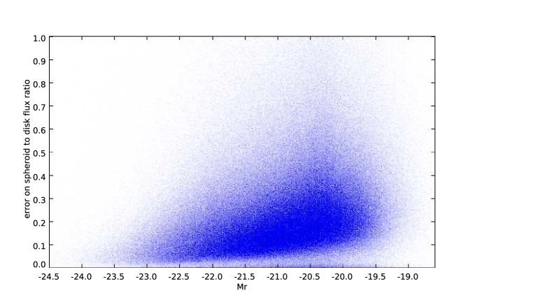
Figure 11: Relative error on the spheroid to total flux ratio as a function of magnitude for all the galaxies in a 1 Mpc radius within clusters at redshift $0.4\leq z<0.75$.

Before stacking clusters and searching for variations of galaxy morphologies with redshift, it is necessary to make a cut in absolute magnitude in order to have comparable samples in all the redshift bins. We make the choice of the limiting magnitude by considering the redshift range that imposes the strongest constraints on the relative uncertainty on the spheroid-to-total ratio: $0.4\leq z<0.75$. A plot of this uncertainty as a function of absolute magnitude for all the cluster galaxies in the redshift range $0.4\leq z<0.75$ is shown in Fig. 11. We choose to limit the relative uncertainty on the spheroid to total flux ratio to 20% and to cut the sample at ${\rm M_{r}\leq-19.0}$ (which roughly corresponds to $M^{*}+3$). Out of the initial sample of 1,574,505 galaxies, there are 1,128,389 galaxies with ${\rm M_{r}\leq-19.0}$, of which 522,605 have an uncertainty $err_{fluxratio}$ on the spheroid-to-total flux ratio smaller than or equal to 20%. So for $M_{r}\leq-19.0$ we can consider that about 50% of the galaxies have $err_{fluxratio}\leq$20%. Hereafter we will take into account only the galaxies with an absolute magnitude brighter than ${\rm M_{r}<-19.0}$.

In the following analysis, we will limit our analysis to the 2530 clusters detected at a 4$\sigma$ level and above to have a sample of clusters that is as reliable as possible. We stacked clusters in six redshift bins: $z\leq 0.15$, $0.15<z\leq 0.25$, $0.25<z\leq 0.35$, $0.35<z\leq 0.45$, $0.45<z\leq 0.55$, and $z>0.55$ and computed the percentages of late-type galaxies. If we assume that there is no observational bias due to the loss of spatial resolution for galaxies when redshift increases, we find that the percentage of late-type galaxies tends to decrease with redshift, opposite to what is expected. We also stacked clusters in four bins of detection level: 4$\sigma$, 5$\sigma$, 6$\sigma$, and 9$\sigma$, which roughly correspond to cluster mass bins. Here too, we tend to find that the percentage of late-type galaxies somewhat increases with significance level, the opposite of what is expected (more massive clusters are expected to host more early-type galaxies). We therefore performed simulations to test the hypothesis that these unexpected results could be due to an observational bias.

6.2 Influence of the redshift on the morphological classification

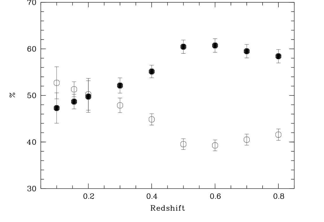
Figure 12: Percentage of early-type galaxies (filled black circles) and late-type galaxies (empty black circles) as a function of redshift obtained by stacking 103 clusters artificially degraded to mimic the influence of increasing redshift (see Section 6.2).

In order to test how the image degradation due to increasing redshift could influence the value of the $f_{spheroid}/(f_{disk}+f_{spheroid})$ flux ratio on which our late- and early-type galaxy percentages are based, we selected 103 clusters with redshift $z\leq 0.20$ and detected at least at the $4\sigma$ level. Starting from the original images, we artificially degraded the images by rebinning them to larger pixel sizes to mimic the effect of increasing redshift. In this way images were computed to simulate the clusters as if they were located at redshifts between 0.2 and 0.8, in bins of 0.1 in redshift. The rebinned images were then treated with SExtractor as above to compute the $f_{spheroid}/(f_{disk}+f_{spheroid})$ flux ratios of all the cluster galaxies.

The percentages of late- and early-type galaxies were then stacked in redshift bins, and the results are shown in Fig. 12. This figure clearly shows that, as a bias due to redshift, the percentage of late-type galaxies tends to decrease with redshift and that of early types to increase. Therefore, when estimating the early-to-late-type ratio, a correcting factor must be applied to correct for this bias. The number of late-type galaxies for various redshifts is given in Table 5. We note that we only consider here cluster galaxies, for which the computed absolute magnitudes take into account the k-corrections and luminosity distance corrections.

Table 5: Percentage of late-type galaxies as a function of redshift obtained by degrading the images to mimic the effect of increasing redshift, as explained in the text.

Redshift	% of late types	number of galaxies
0.1	52.7	4005
0.155	51.3	17824
0.2	50.2	3893
0.3	47.9	17543
0.4	44.9	27283
0.5	39.5	26191
0.6	39.3	25895
0.7	40.5	25652
0.8	41.6	25003

6.3 Results

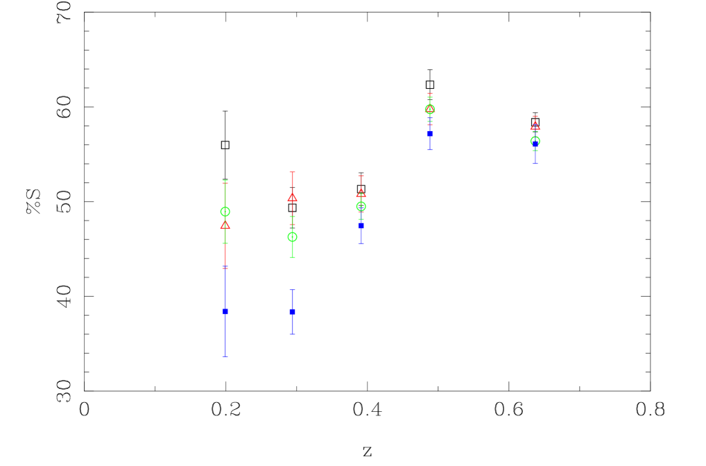
Figure 13: Percentage of late-type galaxies as a function of redshift, based on the bulge to disk decomposition in the $r^{\prime}$ band. The data points are colour–coded as a function of detection level: black circles for 4$\sigma$, red triangles for 5$\sigma$, green circles for 6$\sigma$, and blue squares for 9$\sigma$. The correction factors explained in the text have been applied.

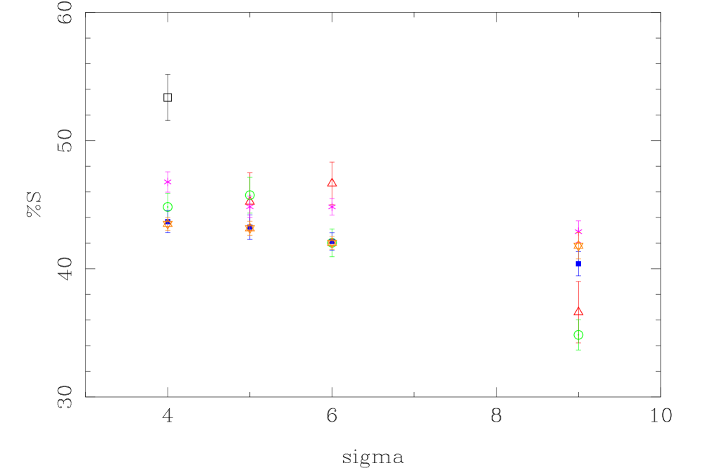
Figure 14: Percentage of late-type galaxies as a function of detection level, based on the bulge to disk decomposition in the $r^{\prime}$ band. The data points are colour–coded in bins of redshift: black squares for $z\leq 0.2$, red triangles for $0.2<z\leq 0.27$, green circles for $0.27<z\leq 0.37$, blue squares for $0.37<z\leq 0.47$, magenta crosses for $0.47<z\leq 0.57$, and orange stars for $z>0.57$. The correction factors explained in the text have been applied.

If we apply the correction factors derived from Table 5 to the percentages of late-type and early-type cluster galaxies found above, we obtain the results displayed in Figs. 13 and 14. In these two figures, the error bars were taken to be Poissonian: $\sqrt{N}/N$, where N is the number of early-type galaxies corresponding to each point.

We can see that the percentages of late-type galaxies increase with redshift. This is particularly visible for 9$\sigma$ clusters, where the percentage of late types increases from 20% to almost 60% between redshifts z=0.2 and z=0.5.

The percentages of late-type galaxies show a trend of decreasing with detection level (i.e. with cluster mass). We note that the percentages of late-type galaxies that we find are notably higher than those of Postman et al. (2005) or Smith et al. (2005) perhaps because our classification of late- and early-type galaxies is not the same, and/or because our cluster galaxies are probably at least partly contaminated by field galaxies.

6.4 Comparison of the galaxy type classifications by SExtractor and Le Phare

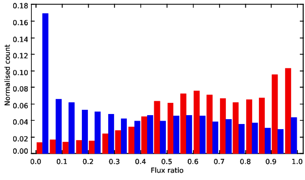
Figure 15: Histograms of the normalized counts of late-type (in blue) and early-type (in red) galaxies as classified by Le Phare, as a function of spheroid-to-disk flux ratio.

Since we had to run the Le Phare software to compute the absolute magnitudes of the cluster galaxies in order to calculate GLFs, as a by-product we obtained a Le Phare galaxy type classification (the same one as that used in the COSMOS survey). Le Phare assigns each galaxy a type coded as a number between 1 and 31, with early-type galaxies between 1 and 7, late-type galaxies between 8 and 19, and AGN between 20 and 31. These types correspond to the best spectral template allowing a fit to the photometric data.

The early- and late-type classifications that we made with SExtractor based on pure morphological properties are not expected to match exactly those derived with Le Phare. However, we believe it is interesting to compare them on a large statistical basis.

If we take into account all the cluster galaxies (77,162 galaxies), we find that 70% of the early-type and 53% of the late-type galaxies have the same classification with the two methods, after eliminating the AGN and starburst types from Le Phare (which add noise to the final morphological classification).

We cross-identified the cluster galaxies with the spectroscopic catalogue described in Section 2.1. The sample is then reduced to only 8,105 galaxies. For this sample, we find that 74% of the early-type galaxies are well classified by both methods, 61% of the late types and 68% if we add late types and AGN.

As a test, we also considered 73,970 galaxies in the Stripe 82 region having a spectroscopic redshift available, independent of whether they were cluster galaxies or not. We ran Le Phare on those galaxies, fixing their photo$-z$ to be equal to their spectroscopic redshift to obtain the best possible Le Phare type. We find that 69% of the early-type and 58% of the late-type galaxies have the same classification with Le Phare and SExtractor. This percentage becomes 63% if we add late types and AGN.

As an illustration, we show in Fig. 15 the histograms of the normalized counts of late- and early-type galaxies as classified by Le Phare as a function of spheroid-to-disk flux ratio computed by SExtractor.

Since these two ways of classifying galaxies are very different from one another (one being purely morphological while the other is purely spectral), and since morphological and spectral evolutions can also be quite different, it is rather satisfying to see that they agree between 58% and 74% of the cases.

6.5 Eye-test of the morphological classification

In order to test the morphological classification obtained with SExtractor, six high school students (see their names in the acknowledgements) selected about 1000 galaxies in the redshift range $0.15<z<0.25$ classified as early-type or late-type and examined them visually with ds9 one by one. They found that the SExtractor and eye classifications agreed for $80\pm$10% of the galaxies.

7 Summary and conclusions

Based on the galaxy photometric redshift catalogue of Reis et al. (2012), we have searched for galaxy clusters in the Stripe 82 region of the Sloan Digital Sky Survey by applying the AMACFI cluster finder (Adami & Mazure 1999). After making nine tests with different AMACFI parameters that have a strong influence on the cluster detection rate, we detected 3663 candidate clusters at a 3$\sigma$ level and above, in the redshift range $0.1\leq z\leq 0.7$, with estimated mean masses between $\sim 10^{13}$ and a few 10¹⁴ M_⊙. We cross-correlated our catalogue of candidate clusters with various catalogues extracted from optical and/or X-ray data. The percentages of redetected clusters are at most 40%, but in all cases this can be explained by the fact that we detect relatively massive clusters, while other authors detect less massive structures.

The colour-magnitude diagrams and galaxy luminosity functions of the clusters detected at 5$\sigma$ and above and stacked in redshift bins of width 0.1 are typically those of bona fide clusters. This confirms that the clusters we have detected have a high probability of being real clusters.

The morphological analysis of the cluster galaxies shows that the fraction of late-type to early-type galaxies shows an increase with redshift and a decrease with significance level, i.e. cluster mass. This result is obtained after correcting for a bias due to the effect of increasing redshift that we quantified through simulations.

Although the 3663 candidate clusters detected here seem mostly to be real clusters, spectroscopic confirmation would of course be necessary. We are in the process of improving the positions and redshifts of our clusters by searching for the brightest cluster galaxies, and retrieving spectroscopic redshifts in the SDSS data base. As yet another confirmation to the reality of the clusters detected in S82, we are also identifying our candidate clusters with diffuse X-ray sources detected by XMM-Newton when available. These results will be published in a forthcoming paper.

Counting the number of clusters per unit volume and the growth of clusters with redshift are methods for delimiting cosmological model parameters such as $w$, $dw/dz$, and $\sigma_{8}$ (Allen et al. 2011). This motivated the present search for clusters in the Stripe 82 region of the SDSS, as well as our previous searches for clusters in the CFHTLS. In the near future, the Dark Energy Survey expects to find approximately 170,000 clusters with masses $\geq 5\times 10^{13}$ M_⊙ (http://en.wikipedia.org/wiki/The_Dark_Energy_Survey), and LSST more than 100,000 clusters with masses $\geq 2\times 10^{14}$ M_⊙ (Tyson et al. 2003).

Based on our experience here, we conclude that is it very important not to depend on using just one cluster detection algorithm. Therefore, for future surveys we suggest the following approach to derive cosmological parameters from optical/near IR cluster surveys: 1) take a $\sim 6\sigma$ cut and a $\sim 4\sigma$ cut; and 2) estimate the completeness of the survey by comparing two or more different cluster finding techniques. The derived cosmological parameters based on two (or more) different $\sigma$ cuts and techniques can then be used to determine the underlying systematic limits to the values of these cosmological parameters.

Appendix A Magnitude histograms

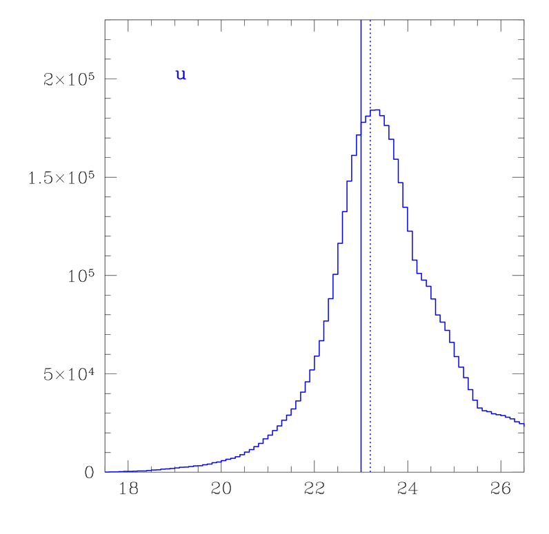
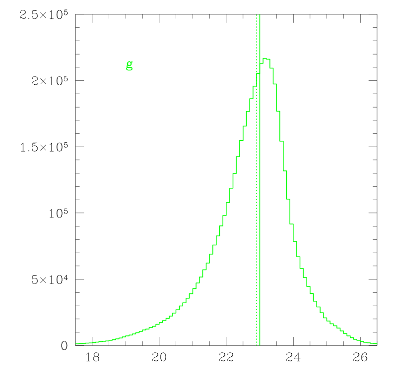
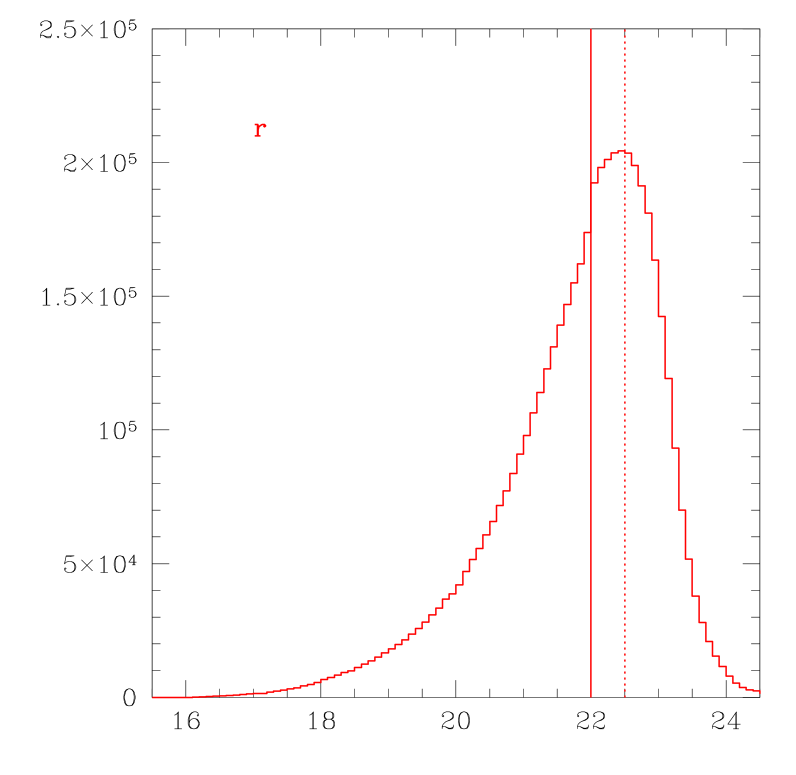
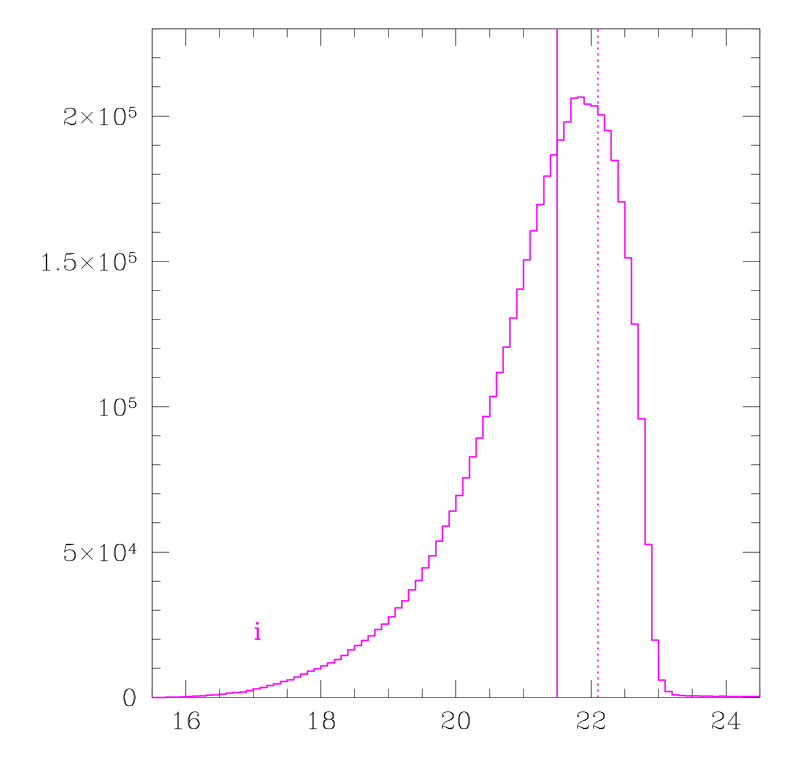
Figure 16: Magnitude histograms in the five bands of the 4,999,968 galaxies of the initial magnitude catalogue used to compute absolute magnitudes. The full vertical lines show the 90% completeness limits beyond which the galaxy counts will not be considered as fitting the GLFs. These limits are: $u^{\prime}_{lim}$=23.0, $g^{\prime}_{lim}$=22.8, $r^{\prime}_{lim}$=22.1, $i^{\prime}_{lim}$=21.5, and $z^{\prime}_{lim}$=21.2. The dotted vertical lines show the 90% completeness limits derived from Fig. 8 in Annis et al. (2014) for comparison.

The magnitude histograms in the five bands of the 4,999,968 galaxies of the initial magnitude catalogue used to compute absolute magnitudes are shown in Fig. 16.

Appendix B Completeness simulations

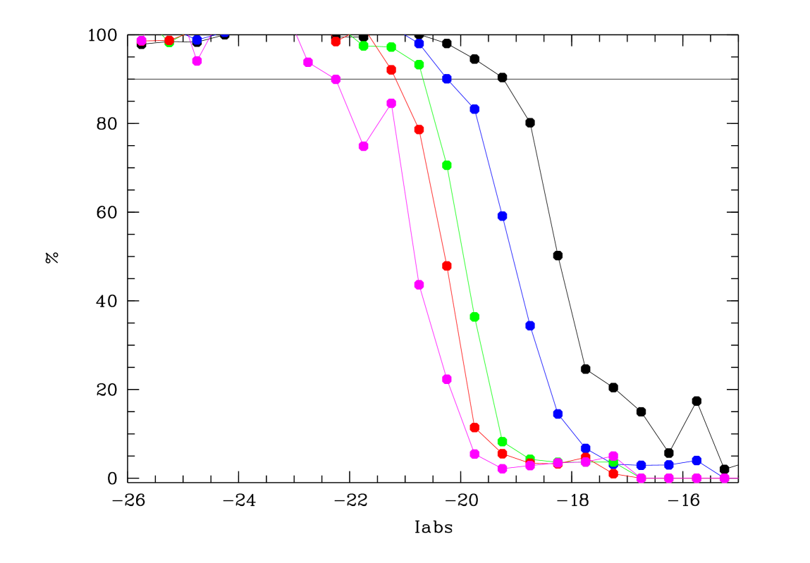
Figure 17: Percentage of redetected galaxies as a function of absolute magnitude in the $i^{\prime}$ band derived from our simulations in five magnitude bins: z=0.2 in black, z=0.3 in blue, z=0.4 in green, z=0.5 in red, and z=0.6 in magenta (see Section 5.2.1).

We show in Fig. 17 the percentages of redetected galaxies as a function of absolute magnitude in the $i^{\prime}$ band derived from our simulations in five magnitude bins: z=0.2 in black, z=0.3 in blue, z=0.4 in green, z=0.5 in red, and z=0.6 in magenta (see Section 5.2.1). Simulations in the other bands give comparable curves and are not shown here to save space.