Exploration of models for a
cargo assembly planning problem

Abstract

We consider a real-world cargo assembly planning problem arising in a coal supply chain. The cargoes are built on the stockyard at a port terminal from coal delivered by trains. Then the cargoes are loaded onto vessels. Only a limited number of arriving vessels is known in advance. The goal is to minimize the average delay time of the vessels over a long planning period. We model the problem in the MiniZinc constraint programming language and design a large neighbourhood search scheme. The effects of various optional constraints are investigated. Some of the optional constraints expand the model’s scope toward a system view (berth capacity, port channel). An adaptive scheme for a greedy heuristic from the literature is proposed and compared to the constraint programming approach.

Keywords: packing, scheduling, resource constraint, large neighbourhood search, constraint programming, adaptive greedy, visibility horizon

1 Introduction

The Hunter Valley Coal Chain (HVCC) refers to the inland portion of the coal export supply chain in the Hunter Valley, New South Wales, Australia. Most of the coal mines in the Hunter Valley are open pit mines. The coal is mined and stored either at a railway siding located at the mine or at a coal loading facility used by several mines. The coal is then transported to one of the terminals at the Port of Newcastle, almost exclusively by rail. The coal is dumped and stacked at a terminal to form stockpiles. Coal from different mines with different characteristics is ‘mixed’ in a stockpile to form a coal blend that meets the specifications of a customer. Once a vessel arrives at a berth at the terminal, the stockpiles with coal for the vessel are reclaimed and loaded onto the vessel. The vessel then transports the coal to its destination. The coordination of the logistics in the Hunter Valley is challenging as it is a complex system involving 14 producers operating 35 coal mines, over 30 coal load points, 2 rail track owners, 4 above rail operators, 3 coal loading terminals with a total of 9 berths, and 9 vessel operators. Approximately 2000 vessels are loaded at the terminals in the Port of Newcastle each year. For more information on the HVCC see the overview presentation of the Hunter Valley Coal Chain Coordinator (HVCCC), the organization responsible for planning the coal logistics in the Hunter Valley [7].

We focus on the management of a stockyard at a coal loading terminal, although we also propose model extensions looking at the processes outside the terminal. An important characteristic of a coal loading terminal is whether it operates as a cargo assembly terminal or as a dedicated stockpiling terminal. When a terminal operates as a cargo assembly terminal, it operates in a ‘pull-based’ manner, where the coal blends assembled and stockpiled are based on the demands of the arriving ships. When a terminal operates as dedicated stockpiling terminal, it operates in a ‘push-based’ manner, where a small number of coal blends are built in dedicated stockpiles and only these coal blends can be requested by arriving vessels.

We focus on cargo assembly terminals as they are more difficult to manage due to the large variety of coal blends that needs to be accommodated. Depending on the size and the blend of a cargo, the assembly may take anywhere from three to seven days. This is due, in part, to the fact that mines can be located hundreds of miles away from the port and getting a trainload of coal to the port takes a considerable amount of time. Once the assembly of a stockpile has started, it is rare that the location of the stockpile in the stockyard is changed; relocating a stockpile is time-consuming and requires resources that can be used to assemble or reclaim other stockpiles. Thus, deciding where to locate a stockpile and when to start its assembly is critical for the efficiency of the system. Ideally, the assembly of the stockpiles for a vessel completes at the time the vessel arrives at a berth (i.e., ‘just-in-time’ assembly) and the reclaiming of the stockpiles commences immediately. Unfortunately, this does not always happen due to the limited capacities of the resources in the system, e.g., stockyard space, stackers, and reclaimers, and the complexity of the stockyard planning problem.

Our cargo assembly planning approach aims to minimize the delay of vessels, where the delay of a vessel is defined as the difference between the vessel’s departure time and its earliest possible departure time, that is, the departure time in a system with infinite capacity. Minimizing the delay of vessels is used as a proxy for maximizing the throughput, i.e., the maximum number of tons of coal that can be handled per year, which is of crucial importance as the demand for coal is expected to grow substantially over the next few years. We investigate the value of information given by the visibility horizon — the number of future vessels whose arrival time and stockpile demands are known in advance.

Despite their economic importance, there is very little literature on coal, and more generally mineral, supply chains. Boland and Savelsbergh [5] discuss a variety of planning problems encountered in the HVCC. Singh et al. [20] discuss expansion planning for the HVCC. Thomas et al. [21] explore integrated planning and scheduling of coal supply chains. Gulzynsky et al. [4] present stockyard management technology which combines greedy construction, enumeration, and integer programming. The closest work to what we describe here is that of Savelsbergh and Smith [15], who propose a greedy algorithm with partial lookahead and truncated tree search using geometric properties of the space-time layouts, for the same stockyard planning problem. We propose a Constraint Programming (CP)-based approach and directly compare it with and extend theirs. The core of our paper, namely the basic CP model and comparison with [15], was presented in the CPAIOR’14 paper [3].

There are obvious links between stockyard management and 2-dimensional bin or strip packing problems (see Lodi et al. [9] for a recent survey). The main difference is that in stockyard management, the length of a rectangular item in one of its dimensions (the time dimension) is not known in advance, but depends on other decisions. Bay et al. [1] consider a shipping yard planning problem where large 2-dimensional blocks need to be handled. They solve this as a 3-dimensional bin packing problem in which one dimension is time.

The solving technology we apply is Constraint Programming using Lazy Clause Generation (LCG) [12]. Constraint programming has been highly successful in tackling complex packing and scheduling problems [18, 19]. CP allows modeling optimization problems at higher level and the flexible addition of new constraints without changing the base model; it also allows the modeller to make use of their knowledge about where good solutions are likely to be found by programming the search strategy. Lazy Clause Generation [11] is a new constraint programming solving technology that allows the solver to “learn” from failures in the search process. It often exponentially improves upon standard CP technology. It is the state-of-the-art on many well-studied scheduling problems and some packing problems. Cargo assembly is a combined scheduling and packing problem. The specific problem is first described by Savelsbergh and Smith [15]. They propose a greedy heuristic for solving the problem and investigate some options concerning various characteristics of the problem. We present a Constraint Programming model implemented in the MiniZinc language [10]. To solve the model efficiently, we develop iterative solving methods: greedy methods to obtain initial solutions and large neighbourhood search methods [14] to improve them. The CP technology facilitates investigation of new practically relevant constraints and their impacts on the solutions. In particular, we extend the model’s scope by a port channel constraint which is modeled as a series of global $\operatorname{\texttt{disjunctive}}$ constraints. Finally, we propose an iterative adaptive scheme which uses the greedy heuristic from [15] as a core component and compare both approaches.

The remainder of the paper is organized as follows. Section 2 describes the problem in detail and reviews the new constraints we investigate with CP technology. Section 3 describes the Constraint Programming model and iterative methods based on it. Section 4 presents an adaptive greedy scheme for the heuristic found in the literature. Experiments are discused in Section 5 and finally in Section 6 we conclude.

2 Cargo assembly planning: overview

The starting point for this work is the model developed in [15] for stockyard planning. The model is described in the next subsection and summarised in Subsection 2.2. We consider a number of constraints beyond those in [15], which are discussed in Subsection 2.3.

2.1 Cargo assembly environment

The stockyard studied has four pads, A, B, C, and D, on which cargoes are assembled. Coal arrives at the terminal by train. Upon arrival at the terminal, a train dumps its contents at one of three dump stations. The coal is then transported on a conveyor to one of the pads where it is added to a stockpile by a stacker. There are six stackers, two that serve pad A, two that serve both pads B and C, and two that serve pad D. A single stockpile is built from several train loads over several days. After a stockpile is completely built, it dwells on its pad for some time (perhaps several days) until the vessel onto which it is to be loaded is available at one of the berths. A stockpile is reclaimed using a bucket-wheel reclaimer and the coal is transferred to the berth on a conveyor. The coal is then loaded onto the vessel by a shiploader. There are four reclaimers, two that serve both pads A and B, and two that serve both pads C and D. Both stackers and reclaimers travel on rails at the side of a pad. Stackers and reclaimers that serve the same pads cannot pass each other. A scheme of the stockyard is given in Figure 1.

Figure 1: A scheme of the stockyard with 4 pads, 6 stackers, and 4 reclaimers

A brief overview of the events driving the cargo assembly planning process is presented next. An incoming vessel alerts the coal chain managers of its pending arrival at the port. This announcement is referred to as the vessel’s nomination. Upon nomination, a vessel provides its estimated time of arrival (ETA) and a specification of the cargoes to be assembled to the coal chain managers. As coal is a blended product, the specification includes for each cargo a recipe indicating from which mines coal needs to be sourced and in what quantities (this is beyond our current scope however). At this time, the assembly of the cargoes (stockpiles) for the vessel can commence. A vessel cannot arrive at a berth prior to its ETA, and often a vessel has to wait until after its ETA for a berth to become available. Once at a berth, and once all its cargoes have been assembled, the reclaiming of the stockpiles (the loading of the vessel) can begin. A vessel must be loaded in a way that maintains its physical balance in the water. As a consequence, for vessels with multiple cargoes, there is a predetermined sequence in which its cargoes must be reclaimed. The goal of the planning process is to maximize the throughput without causing unacceptable delays for the vessels.

For a given set of vessels arriving at the terminal, the goal is thus to assign each cargo of a vessel to a location in the stockyard, schedule the assembly of these cargoes, and schedule the reclaiming of these cargoes, so as to minimize the average delay of the vessels, where the delay of a vessel is defined to be the difference between the departure time of the vessel (or equivalently the time that the last cargo of the vessel has been reclaimed) and the earliest time the vessel could depart under ideal circumstances, i.e., the departure time if we assume the vessel arrives at its ETA and its stockpiles can be reclaimed immediately upon its arrival.

When assigning each cargo of a vessel to a location in the stockyard, scheduling the assembly of these cargoes, and scheduling the reclaiming of these cargoes, we account for limited stockyard space, stacking rates, reclaiming rates, and reclaimer movements, but we assume that other parts of the system have infinite capacity and thus do not restrict our decisions. The reason for doing so is that our industry partner believes that the stockyard is, or will soon be, the bottleneck in the system and that the other parts of the system can be managed in such a way that they adjust to what is needed to operate the stockyard as effectively as possible. Consequently, we assume that coal is available for stacking any time, and that a vessel is at berth and can be loaded whenever we want to reclaim a stockpile.

We model stacking and reclaiming at different levels of granularity. Since reclaimers are most likely to be the constraining entities in the system, we model reclaimer activities at a fine level of detail. That is, all reclaimer activities, e.g., the reclaimer movements along its rail track and the reclaiming of a stockpile, are modelled in time units of one minute. On the other hand, we model stacking at a coarser level of detail. First, we assume that the time it takes to build a stockpile can be derived from its constituent components. As the constituent components define the mines from which the coal will be sourced, this is not unreasonable. The distance from the terminal to the mine determines the cycle time of the trains used to transport the coal and thus stockpiles with coal sourced from mines that are far away from the terminal tend to take longer to build. Second, we consider stacking capacity at an aggregate daily level for each pair of stackers serving the same pads. As each pair of stackers is linked by a conveyor system to a particular dump station at the terminal, often referred to a stacking stream, this is not unreasonable.

When deciding a stockpile location, a stockpile stacking start time, and a stockpile reclaiming start time, a number of constraints have to be taken into account: at any point in time no two stockpiles can occupy the same space on a pad, reclaimers cannot be assigned to two stockpiles at the same time, reclaimers can only be assigned to stockpiles on pads that they serve, reclaimers serving the same pads cannot pass each other, the stockpiles of a vessel have to be reclaimed in a specified reclaim order and the time between the reclaiming of consecutive stockpiles of a vessel can be no more than a prespecified limit, the so-called continuous reclaim time limit, and, finally, the reclaiming of the first stockpile of a vessel cannot start before all stockpiles of that vessel have been stacked. We assume that the rate of reclaiming is the same for all reclaimers, and thus that the time it takes to reclaim a given stockpile can be calculated from its size, which is a reasonable model of the real situation.

A cargo assembly plan can conveniently be represented using space-time diagrams; one space-time diagram for each of the pads in the stockyard. A space-time diagram for a pad shows for any point in time which parts of the pad are occupied by stockpiles (and thus also which parts of the pad are not occupied by stockpiles and are available for the placement of additional stockpiles) and the locations of the reclaimers serving that pad. Every pad is rectangular; however its width is much smaller than its length and each stockpile is spread across the entire width. Thus, we model pads as one-dimensional entities. The location of a stockpile can be characterized by the position of its lowest end called its height. A stockpile occupies space on the pad for a certain amount of time. This time can be divided into three distinct parts: the stacking part, i.e., the time during which the stockpile is being built; the dwell part, i.e., the time between the end of stacking and the start of reclaiming; and a reclaiming part, i.e., the time during which the stockpile is reclaimed and loaded on a waiting vessel at a berth. We assume that a stockpile’s reclaim process, reclaim job, cannot be interrupted. Thus, each stockpile can be represented in a space-time diagram by a three-part rectangle as shown in Figure 2.

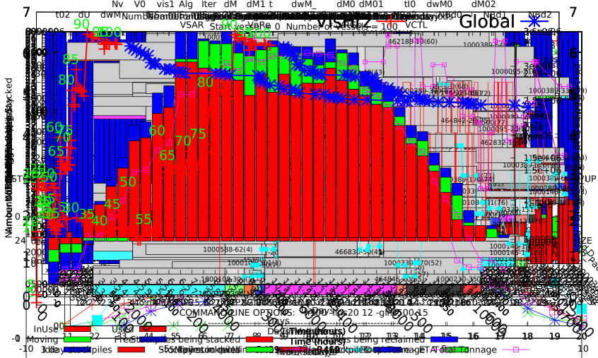
Figure 2: A space-time diagram of pad A showing also reclaimer movements. Reclaimer R459 has to be after R460 on the pad. Both reclaimers also have jobs on pad B.

2.2 The basic model

Based on the above description of the problem, we summarize the important features of the model studied in [15], which is taken as the basic model here.

• 4 pads, arranged in parallel, 4 reclaimers (2 between each pair of pads).

• 3 stacker streams, (one each for the outer pads, one for the two inner), each with capacity 288,000 t/day and overall capacity (maximum daily inbound throughput, DIT) 537,600 t/day.

• Stacking duration 3/5/7 days for each stockpile, which is reflective of what happens in real life.

• The stacking volume of each stockpile is evenly divided over the stacking period.

• Stacking of a stockpile can start at most 10 days before the ETA of its vessel.

• Reclaimer’s travel speed: 30 meters per minute.

• Reclaim the stockpiles of each vessel in given order, one stockpile at a time.

• Reclaim job of any stockpile is non-interruptible.

• Continuous reclaim limit (i.e., maximal time between reclaiming) for two consecutive stockpiles of a vessel: 5 hours.

• Same pad is used for all stockpiles of a single vessel. While not the industrial practice, this rule produced better solutions both in [15] and in our experiments, so we include it into the basic model and present its impact in the numerical results.

The goal is to minimize the average delay of all vessels.

In [15] the authors do not consider the delay of the first and last 8 vessels. The reason is that these vessels have more placement freedom and thus easy to schedule. In our experiments, exclusion of the delays in these ‘warm-up’ and ‘cool-down’ vessels from the objective function made them unreasonably high. That is why we optimize over all vessels, however we report some results taking ‘warm-up’ and ’cool-down’ into account. Moreover, we investigate the effect of a limited visibility horizon, i.e., when the number of the next arriving ships known is limited.

As observed in [15], minimizing dwell (stockpile’s waiting time) after scheduling each stockpile or vessel is generally bad because this reduces resources for later vessels. Thus, we do not consider dwell in the basic model.

2.3 Model extensions

There are many further constraints which are relevant in practice and it is important to investigate their effect on the solutions. We consider the following optional constraints, some of which are a first step toward a system view of the transport chain:

• Different pads allowed for allocation of stockpiles of one and the same vessel.

• Build all stockpiles of a vessel (stack them) before reclaiming any of them.

• Maximal number of simultaneously berthed ships (4).

• Maximal number of reclaimers working at any time (3). This constraint models the fact that only 3 ship loaders are available at the terminal.

• Tidal constraints: big ships are tidally constrained, that is, they can leave the port only during high tides, which for simplicity we model as the periods 11:15–12:45am and 11:15–12:45pm (more accurate modeling would certainly not be too difficult to add). In practice, a ship is considered tidally constrained if its weight is equal to or above 100,000 tonnes.

• Channel constraints: time between any two departures is at least 20 minutes; the same for arrivals. After any departure, the earliest possible arrival is 140 minutes later. The reason is the port entry channel which can let only one vessel in each direction.

• Flexible stacking volumes for each day for a stockpile.

• $\pm$1 day stacking duration for each stockpile.

• Dwell post-processing.

The next section presents a Constraint Programming model of the above problem.

3 The Constraint Programming-based approach

We implemented the model in the MiniZinc language [10] which is accepted by many solvers. As reasoned in Section 2.1, we use a fine and coarse time discretization for modeling reclaiming and stacking, respectively. The non-overlapping of stockpiles in space and time is a three-dimensional diffn constraint [2] where the pad number can be seen as a third dimension. In the solver we use the diffn constraint is implemented by decomposition.

The model extensively uses the constraint

$$\operatorname{\texttt{cumulative}}(t,d,r,R)$$ (1)

restricting the available renewable resource capacity $R$ for jobs with start times, durations, and resource demands given by vectors $t$, $d$, and $r$, respectively [10]. If $d$, $r$, and $R$ are constants, the particular solver we use applies a global version of $\operatorname{\texttt{cumulative}}$, otherwise a decomposed version [17] is used (e.g. for constraint (4c)). A redundant $\operatorname{\texttt{cumulative}}$ constraint (3d) models pad usage, which is known to be important to reduce search space in packing problems [19]. Cumulative constraints are also used to model stacking capacity and, in the extended model (Section 3.2), reclaimer usage.

We also make use of the $\operatorname{\texttt{disjunctive}}$ global constraint which is a specialized form of $\operatorname{\texttt{cumulative}}$.

$$\operatorname{\texttt{disjunctive}}(t,d)=\operatorname{\texttt{cumulative}}(t,d,\mathbf{1},1)$$ (2)

where $\mathbf{1}$ is a vector of 1s, which ensures that no two tasks overlap in time. Constraint programming solvers can more efficiently handle the specialized $\operatorname{\texttt{disjunctive}}$ constraint.

We present the basic model, extended model, solver search strategy, construction of initial solutions, large neighbourhood search, and an approach for limited visibility horizons.

3.1 The basic Constraint Programming model

This subsection models the basic problem subset described in Section 2.2. The presented structure of the constraints corresponds to their implementation in the MiniZinc language, however mathematical notation is used where possible to improve readability. In [15] continuous input data is used. But Constraint Programming solvers concentrate on integer variables, so in the implementation the times are rounded to minutes; distances to whole meters; and stacking tonnages to integers. We round up in order to be conservative. In addition, stacking start times are restricted to be multiples of 12 hours.

• set of stockpiles of all vessels, ordered by vessels’ ETAs and reclaim sequence of each vessel’s stockpiles

• set of vessels, ordered by ETAs

• vessel for stockpile $s\in S$

• estimated time of arrival of vessel $v\in V$, minutes

• reclaiming duration of stockpile $s\in S$, minutes

• length of stockpile $s\in S$, meters

• travel speed of a reclaimer, meters / minute

• daily stacking tonnage of stockpile $s\in S$, tonnes

• daily inbound throughput (total daily stacking capacity), tonnes

• daily capacity of stacker stream $k\in\{1,2,3\}$, tonnes

• pad on which the stockpiles of vessel $v\in V$ are assembled

• position of stockpile $s\in S$ (of its ‘closest to pad start’ boundary) on the pad

• stacking start time of stockpile $s\in S$

• reclaimer used to reclaim stockpile $s\in S$

• reclaiming start time of stockpile $s\in S$

Constraints.

Reclaiming of a stockpile cannot start before its vessel’s ETA:

$$t^{R}_{s}\geq\operatorname{eta}_{v_{s}},\qquad\forall s\in S$$

Stacking of a stockpile starts no more than 10 days before its vessel’s ETA:

$$t^{S}_{s}\geq\operatorname{eta}_{v_{s}}-14400,\qquad\forall s\in S$$

Stacking of a stockpile has to complete before reclaiming can start:

$$t^{S}_{s}+d^{S}_{s}\leq t^{R}_{s},\qquad\forall s\in S$$

The reclaim order of the stockpiles of a vessel has to be respected:

$$t^{R}_{s}+d^{R}_{s}\leq t^{R}_{s+1},\qquad\forall s\in S\text{~{}where~{}}\ v_{s}=v_{s+1}$$

The continuous reclaim time limit of 5 hours has to be respected:

$$t^{R}_{s+1}-300\leq t^{R}_{s}+d^{R}_{s},\qquad\forall s\in S\text{~{}where~{}}\ v_{s}=v_{s+1}$$

A stockpile has to fit on the pad it is assigned to:

$$0\leq h_{s}\leq H_{p_{v_{s}}}-l_{s},\qquad\forall s\in S$$

Stockpiles cannot overlap in space and time:

$$p_{v_{s}}\neq p_{v_{t}}\vee h_{s}+l_{s}\leq h_{t}\vee h_{t}+l_{t}\leq h_{s}\vee t^{R}_{s}+d^{R}_{s}\leq t^{S}_{t}\vee t^{R}_{t}+d^{R}_{t}\leq t^{S}_{s},\\ \forall s<t\in S$$ (3a)

Reclaimers can only reclaim stockpiles from the pads they serve:

$$p_{v_{s}}\leq 2\Leftrightarrow r_{s}\leq 2,\qquad\forall s\in S$$

If two stockpiles $s<t$ are reclaimed by the same reclaimer, then the time between the end of reclaiming the first and the start of reclaiming the second should be enough for the reclaimer to move from the middle of the first to the middle of the second:

$$r_{s}\neq r_{t}\vee\max\bigl{\{}(t^{R}_{t}-t^{R}_{s}-d^{R}_{s}),(t^{R}_{s}-t^{R}_{t}-d^{R}_{t})\bigr{\}}\operatorname{speed}^{R}\geq\Bigl{|}h_{s}+\frac{l_{s}}{2}-h_{t}-\frac{l_{t}}{2}\Bigr{|}$$ (3b)

To avoid clashing, at any point in time, the position of Reclaimer 2 should be before the position of Reclaimer 1 and the position of Reclaimer 4 should be before the position of Reclaimer 3. An example of the position of Reclaimers 1 and 2 in space and time is given in Figure 3 (see also Figure 2).

Figure 3: A schematic example of space (vertical)-time (horizontal) location of Reclaimers 1 and 2 with some reclaim jobs. Reclaimer 2 has to stay spatially before Reclaimer 1.

In Figure 3, because Job 3 is spatially before Job 1, there is no concern for a clash. However, since Job 6 is spatially after Job 2, we have to ensure that there is enough time for the reclaimers to get out of each other’s way. The slope of the dashed line corresponds to the reclaimer’s travel speed ($\operatorname{speed}^{R}$), so we see that the time between the end of Job 6 and the start of Job 2 has to be at least $(h_{6}+l_{6}-h_{2})/\operatorname{speed}^{R}$.

We model clash avoidance by a disjunction: for any two stockpiles $s\neq t$, one of the following conditions must be met: either $(r_{s}\geq 3\wedge r_{t}\leq 2)$, in which case $r_{s}$ and $r_{t}$ serve different pads; or $r_{s}<r_{t}$, in which case $r_{s}$ does not have to be before $r_{t}$; or $h_{s}+l_{s}\leq h_{t}$, in which case stockpile $s$ is before stockpile $t$; or, finally, enough time between the reclaim jobs exists for the reclaimers to get out of each other’s way:

$$\max\bigl{\{}(t^{R}_{t}-t^{R}_{s}-d^{R}_{s}),(t^{R}_{s}-t^{R}_{t}-d^{R}_{t})\bigr{\}}\operatorname{speed}^{R}\geq h_{s}+l_{s}-h_{t}\\ \vee r_{s}<r_{t}\vee(r_{s}\geq 3\wedge r_{t}\leq 2)\vee h_{s}+l_{s}\leq h_{t},\quad\forall s\neq t\in S$$ (3c)

Redundant cumulatives on pad space usage improved efficiency. They require derived variables $l^{p}_{s}$ giving the ‘pad length of stockpile $s$ on pad $p$’:

$$l^{p}_{s}=\begin{cases}l_{s},&\text{if }p_{v_{s}}=p,\\ 0,&\text{otherwise},\end{cases}\qquad\forall s\in S,\ p\in\{1,\dots,4\}$$

$$\operatorname{\texttt{cumulative}}(t^{S},t^{R}+d^{R}-t^{S},l^{p},H_{p}),\qquad p\in\{1,\dots,4\}$$ (3d)

The stacking capacity is constrained day-wise. If a stockpile is stacked on day $d$ and the stacking is not finished before the end of $d$, the full daily tonnage of that stockpile is accounted for using derived variables

$$t^{S1}=\lfloor t^{S}/1440\rfloor,\quad d^{S1}=\lfloor d^{S}/1440\rfloor$$

The daily stacking capacity cannot be exceeded:

$$\operatorname{\texttt{cumulative}}(t^{S1},d^{S1},\operatorname{tonn}^{\text{daily}},\operatorname{tonn}^{\text{DIT}})$$

The capacity of stacker stream $k$ (a set of two stackers serving the same pads) is constrained similar to pad space usage:

$$\operatorname{tonn}^{\text{daily}}_{ks}=\begin{cases}\operatorname{tonn}^{\text{daily}}_{s},&\text{if }(p_{v_{s}},k)\in\{(1,1),(2,2),(3,2),(4,3)\}\\ 0,&\text{otherwise},\end{cases}\qquad\forall s,k$$

$$\operatorname{\texttt{cumulative}}(t^{S1},d^{S1},\operatorname{tonn}^{\text{daily}}_{k},\operatorname{tonn}^{\text{SS}}_{k}),\qquad k\in\{1,2,3\}$$

Objective function.

The objective is to minimize the sum of vessel delays. To define vessel delays, we introduce the derived variables $t^{\text{Depart}}_{v}$ for vessel departure times:

$$\operatorname{depEarliest}_{v} =\operatorname{eta}_{v}+\sum_{s|v_{s}=v}d^{R}_{s},\qquad \forall v\in V$$ (3e)

$$t^{\text{Depart}}_{v} =t^{R}_{s^{\text{last}}(v)}+d^{R}_{s^{\text{last}}(v)},\qquad s^{\text{last}}(v)=\max\{s|v_{s}=v\},\quad\forall v\in V$$ (3f)

$$\operatorname{delay}_{v} =t^{\text{Depart}}_{v}-\operatorname{depEarliest}_{v},\qquad \forall v\in V$$ (3g)

objective $$=\sum_{v}\operatorname{delay}_{v}$$ (3h)

Except for the discretizations, the above model corresponds to that used in [15]. The differences are once more summarized in Section 4.2.

3.2 Model extensions

Constraint programming models allow relatively easy addition of further constraints and options to the model, either detailing stockyard operation or leading to a more global view of the system. Below we explain and define them.

Different pads for stockpiles of one vessel allowed:

instead of the variables $p_{v}$ denoting the pad used to allocate the stockpiles of vessel $v\in V$, implement $p_{s}$ for each stockpile $s\in S$.

Stack all before reclaim:

Build all stockpiles of a vessel (stack them) before reclaiming any of them.

$$t^{S}_{s}+d^{S}_{s}\leq t^{R}_{s^{\text{first}}(v)},\quad\forall v_{s}=v:s\neq s^{\text{first}}(v)=\min\{s|v_{s}=v\},\ \forall v\in V$$ (4a)

Berth capacity:

Maximal number of simultaneously berthed ships is 4. We introduce derived variables for vessels’ berth arrivals and use a decomposed cumulative:

$$t^{\text{Berth}}_{v}=t^{R}_{s^{\text{first}}(v)},\qquad\forall v\in V$$ (4b)

$$\operatorname{card}(\{u\in V\ |\ u\neq v,\ t^{\text{Berth}}_{u}\leq t^{\text{Berth}}_{v}\wedge t^{\text{Berth}}_{v}<t^{\text{Depart}}_{u}\})\leq 3=4-1,\qquad\forall v\in V$$ (4c)

Ship loading capacity:

Maximal number of reclaimers working at any time is 3. This can be easily imposed by a global cumulative:

$$\operatorname{\texttt{cumulative}}(t^{R},d^{R},\mathbf{1},3)$$ (4d)

Tidal constraints:

Ships exceeding certain weight limit can leave the port only during the high tides 11:15–12:45am and 11:15–12:45pm. The berth is allocated until departure.

Modeling: the departure time variables $t^{\text{Depart}}_{v}$ (3f) for tidal vessels are disconnected from the end of reclaiming by changing the equalities (3f) to ‘greater-or-equal’. The domains of these variables are set as the tidal windows. Moreover, the constant representing earliest possible departure (3e) and used to compute actual delay (3g) is increased to the next tidal window boundary if it is not already inside a tidal window.

Channel constraint:

time between any two departures is at least 20 minutes; the same for arrivals. After any departure, the earliest possible arrival is 140 minutes later. The channel constraint can be illustrated in a space-time diagram representing vessels’ positions in the channel depending on time. To pass through the channel in any direction, a vessel needs 60 minutes. Moreover, before a new vessel can enter, the last exiting vessel needs at least 20 more minutes to clear the entrance area. We can represent arrivals and departures by polygons in a space-time diagram. The left-hand side of a polygon represents a vessel’s movement. The polygons have time spans 60 and 80 for arrival and departure, respectively, and ‘thickness’ 20 to ensure the distance between vessels going in one direction. This gives a polygon packing problem exemplified in Figure 4. We don’t use this analogy for our modeling, however.

Figure 4: Channel constraint as a polygon packing problem, $t^{A}$ standing for time of arrival (berth time) and $t^{D}$ for time of departure

Modeling: the departure time variables $t^{\text{Depart}}_{v}$ (3f) for all vessels are disconnected from the end of reclaiming by changing the equalities (3f) to ‘greater-or-equal’. Similarly, the arrival time variables $t^{\text{Berth}}_{v}$ (4b) are disconnected from the start of reclaiming, demanding to be earlier or simultaneously. The process of entering or leaving the port for each vessel is partitioned in 20-minute intervals and some of these intervals are demanded to be disjunct among different vessels.

In detail, we represent the departure process by four 20-minute jobs $D_{0},D_{20},D_{40},D_{60}$ starting at the following time points:

$$t^{D_{0}}_{v}=t^{\text{Depart}}_{v},\ t^{D_{20}}_{v}=t^{D_{0}}_{v}+20,\ t^{D_{40}}_{v}=t^{D_{0}}_{v}+40,\ t^{D_{60}}_{v}=t^{D_{0}}_{v}+60,\quad\forall v\in V$$ (4e)

Similarly, the arrival process is represented by three 20-minute jobs $A_{60},A_{40},A_{20}$:

$$t^{A_{60}}_{v}=t^{\text{Berth}}_{v}-60,\ t^{A_{40}}_{v}=t^{\text{Berth}}_{v}-40,\ t^{A_{20}}_{v}=t^{\text{Berth}}_{v}-20,\quad\forall v\in V$$ (4f)

According to the assumption, the jobs ${D_{i}}$ of all vessels are all disjoint for a fixed $i\in\{0,20,40,60\}$, as well as jobs $A_{j}$ for a fixed $j\in\{20,40,60\}$. Moreover, any job $D_{i}$ is disjoint from any job $A_{j}$, $\forall i,j$. Let us define vectors $t^{DA}_{ij}\in{\mathbb{Z}}^{2|V|}$ containing the start times of all jobs $t^{D_{i}}$ and $t^{A_{j}}$:

$$t^{DA}_{ij}=\{t^{D_{i}}_{1},\dots,t^{D_{i}}_{|V|},t^{A_{j}}_{1},\dots,t^{A_{j}}_{|V|}\},\qquad i\in\{0,20,40,60\},\ j\in\{20,40,60\}$$

Both restrictions can be modelled by the following 12 disjunctive constraints [10] ensuring disjointness of the jobs:

$$\operatorname{\texttt{disjunctive}}(t^{DA}_{ij},20\times\mathbf{1}),\qquad i\in\{0,20,40,60\},\ j\in\{20,40,60\}$$ (4g)

Note that it is possible to reduce the number of variables and constraints, e.g., by disregarding variables $t^{D_{20}}$ and $t^{D_{40}}$ and the constraints involving them, but this showed no significant speed up in the computational experiments.

Flexible stacking volumes:

we can allow some deviation in the daily stacking portions for each stockpile $s\in S$, let’s say, the fraction of $\delta^{\operatorname{tonn}}\in[0,1)$ of the nominal daily volume $\operatorname{tonn}^{\text{daily}}_{s}$. Thus, we introduce stacking volume variables $v^{s}_{d}$ for each of the stacking days $d\in\bigl{\{}1,\dots,\frac{d^{S}_{s}}{1440}\bigr{\}}$ of each stockpile $s\in S$:

$$v^{\min}_{s} =\lfloor(1-\delta^{\operatorname{tonn}})\operatorname{tonn}^{\text{daily}}_{s}\rfloor,\qquad \forall s\in S$$ (4h)

$$v^{\max}_{s} =\lceil(1+\delta^{\operatorname{tonn}})\operatorname{tonn}^{\text{daily}}_{s}\rceil,\qquad \forall s\in S$$ (4i)

$$\operatorname{stkDays}_{s} =d^{S}_{s}/1440,\qquad \forall s\in S$$ (4j)

$$v^{s}_{1},\ldots,v^{s}_{d} \in\{v^{\min}_{s},\dots,v^{\max}_{s}\},\qquad d\in\{1,\dots,\operatorname{stkDays}_{s}\},\quad \forall s\in S$$ (4k)

$$v^{s}_{1}+\dots+v^{s}_{d} =\operatorname{tonn}^{\text{daily}}_{s}\operatorname{stkDays}_{s},\qquad \forall s\in S$$ (4l)

To formulate a cumulative stacking capacity constraint, we need derived variables for the stacking times:

$$t^{SD}_{sd}=t^{S1}_{s}+d-1,\qquad d\in\{1,\dots,\operatorname{stkDays}_{s}\},\quad\forall s\in S$$ (4m)

Deriving stacking volume variables $v^{sk}_{d}$ for each stream $k\in\{1,2,3\}$ similar to (3.1), we obtain the cumulative capacity constraints

$$\operatorname{\texttt{cumulative}}(t^{SD},\mathbf{1},v,\operatorname{tonn}^{\text{DIT}})$$ (4n)

$$\operatorname{\texttt{cumulative}}(t^{SD},\mathbf{1},v^{k},\operatorname{tonn}^{\text{SS}}_{k}),\qquad k\in\{1,2,3\}$$ (4o)

$\mathbf{\pm}$1 day stacking duration:

we make the upper and lower bounds for daily stack volumes variable (${v^{\min}_{s}}^{\prime}$, ${v^{\max}_{s}}^{\prime}$) and introduce stacking duration variables ${d^{S}_{s}}^{\prime}$ to be used instead of the constants $d^{S}_{s}$:

$$\delta^{-}_{s}=\delta^{\operatorname{tonn}}{{\operatorname{tonn}^{\text{daily}}_{s}}}\frac{\operatorname{stkDays}_{s}}{\operatorname{stkDays}_{s}+1},\qquad\forall s\in S$$ (4p)

$$\delta^{+}_{s}=\delta^{\operatorname{tonn}}{{\operatorname{tonn}^{\text{daily}}_{s}}}\frac{\operatorname{stkDays}_{s}}{\operatorname{stkDays}_{s}-1},\qquad\forall s\in S$$ (4q)

$${v^{\min}_{s}}^{\prime}=\Bigl{\lfloor}{{\operatorname{tonn}^{\text{daily}}_{s}}}\frac{\operatorname{stkDays}_{s}}{{d^{S}_{s}}^{\prime}/1440}\Bigr{\rfloor}-\delta^{-}_{s},\qquad\forall s\in S$$ (4r)

$${v^{\max}_{s}}^{\prime}=\Bigl{\lceil}{{\operatorname{tonn}^{\text{daily}}_{s}}}\frac{\operatorname{stkDays}_{s}}{{d^{S}_{s}}^{\prime}/1440}\Bigr{\rceil}+\delta^{+}_{s},\qquad\forall s\in S$$ (4s)

$${d^{S}_{s}}^{\prime}=\begin{cases}{d}^{S}_{i}+1440,&v^{s}_{\operatorname{stkDays}_{s}+1}\geq\max\{1,{v^{\min}_{s}}^{\prime}\},\\ {d}^{S}_{i},&v^{s}_{\operatorname{stkDays}_{s}}\geq\max\{1,{v^{\min}_{s}}^{\prime}\}\wedge v^{s}_{\operatorname{stkDays}_{s}+1}=0,\\ {d}^{S}_{i}-1440,&v^{s}_{\operatorname{stkDays}_{s}}=v^{s}_{\operatorname{stkDays}_{s}+1}=0,\end{cases}\qquad\forall s\in S$$ (4t)

Dwell post-processing:

Stockpile dwell is the time between stacking and reclaiming when the stockpile just occupies space on the pad. Already in [15] it was found that reducing dwell immediately after placing a stockpile is generally not a good idea because it reduces resources for later stockpiles. In our tests, we even found it advantageous to increase dwell during schedule construction. Thus, we only reduce dwell by post-processing of complete solutions, changing the stacking start times and daily volumes of stockpiles for groups of each 5 vessels.

3.3 Solver search strategy

As discussed below, it is difficult to obtain good solutions by trying to solve a complete problem instance in a single solver call. Instead, we heuristically decompose the problem into smaller parts by visibility horizons and LNS. However, when solving each smaller part, the search strategy of the CP solver is important.

Many Constraint Programming models benefit from a custom search strategy for the solver. Similar to packing problems [6], we found it advantageous to separate branching decisions by groups of variables. We start with the most important variables — departure times of all ships (equivalently, delays). This proved helpful to quickly find good solutions. Then we fix all reclaim starts, pads, reclaimers, stack starts, and pad positions. For most of the variables, we use the dichotomous strategy indomain_split for value selection, which divides the current domain of a variable in half and tries first to find a solution in the lower half. However, pads are assigned randomly, and reclaimers are assigned preferring lower numbers for odd vessels and higher numbers for even vessels. Pad positions are preferred so as to be closer to the native side of the chosen reclaimer, which corresponds to the idea of opportunity costs in [15]. It appears best not to specify any strategy for daily stacking volumes, however we make sure that bigger values are tried first for earlier days. Let us call this strategy LayerSearch(1,…,$|V|$) because we start with all vessels’ departure times, continue with reclaim times, pads, etc. Some experimentation with this strategy is discussed in the results section.

In the greedy and LNS heuristics described next, some of the variables are fixed and the model optimizes only the remaining variables. For those free variables, we apply the search strategy described above.

3.4 Initial feasible solutions: a truncated search heuristic

In one CP solver call, it is difficult to obtain feasible solutions for large instances in a reasonable amount of time. Moreover, even for average-size instances, if a feasible solution is found, it is usually bad. Therefore, we apply a divide-and-conquer strategy which schedules vessels by groups (e.g., solve vessels 1–5, then vessels 6–10, then vessels 11–15, etc.). For each group, we allow the solver to run for a limited amount of time, and, if feasible solutions are found, take the best of these, or, if no feasible solution is found, we reduce the number of vessels in the group and retry. We refer to this scheme as the extending horizon (EH) heuristic. This heuristic is generalized in Section 3.6.

3.5 Large neighbourhood search

After obtaining a feasible solution, we try to improve it by re-optimizing subsets of variables while others are fixed to their current values, a large neighbourhood search approach [14]. We can apply this improvement approach to both complete solutions (global LNS) or only for the current visibility horizon (see Section 3.6). The free variables used in the large neighbourhood search are the decision variables associated with certain stockpiles.

Neighbourhood construction methods. We consider a number of methods for choosing which stockpile groups to re-optimize (the neighbourhoods):

 Spatial

Groups of stockpiles located close to each other on one pad, measured in terms of their space-time location.

 Time-based (finish)

Groups of stockpiles on at most two pads with similar reclaim end times.

 Time-based (ETA)

Groups of stockpiles on at most two pads belonging to vessels with similar estimated arrival times.

Examples of a spatial and a time-based neighbourhood are given in Figure 5.

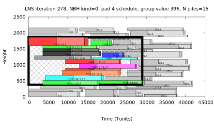
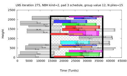
Figure 5: Examples of LNS neighbourhoods: spatial (left) and time-based (right)

First, we randomly decide which of the three types of neighbourhood to use. Next, we construct all neighbourhoods of the selected type. Finally, we randomly select one neighbourhood for resolving.

Spatial neighbourhoods are constructed as follows. In order to obtain many different neighbourhoods, every stockpile seeds a neighbourhood containing only that stockpile. Then all neighbourhoods are expanded. Iteratively, for each neighbourhood, and for each direction right, up, left, and down, independently, we add the stockpile on the same pad that is first met by the sweep line going in that direction, after the sweep line has touched the smallest enclosing rectangle of the stockpiles currently in the neighbourhood. We then add all stockpiles contained in the new smallest enclosing rectangle. We continue as long as there are neighbourhoods containing fewer than the target number of stockpiles.

Time-based neighbourhoods are constructed as follows. Stockpiles are sorted by their reclaim end time or by the ETA of the vessels they belong to. For each pair of pads, we collect all maximal stockpile subsequences of the sorted sequence of up to a target length, with stockpiles allocated to these pads.

Having constructed all neighbourhoods of the chosen type, we randomly select one neighborhood of the set. The probability of selecting a given neighborhood is proportional to its neighborhood value: if the last, but not all stockpiles of a vessel is in the neighborhood, then add the vessel’s delay; instead, if all stockpiles of a vessel are in the neighborhood, then add 3 times the vessel’s delay.

We denote the iterative large neighbourhood search method by LNS$(k_{\max},n_{\max},\delta)$, where for at most $k_{\max}$ iterations, we re-optimize neighborhoods of up to $n_{\max}$ stockpiles chosen using the principles outlined above, requiring that the total delay decreases at least by $\delta$ minutes in each iteration. The objective is again to minimize the total delay (3h).

3.6 Limited visibility horizon

In the real world, only a limited number of vessels is known in advance. We model this as follows: the current visibility horizon is $N$ vessels. We obtain a schedule for the $N$ vessels and fix the decisions for the first $F$ vessels. Then we schedule vessels $F+1,\dots,F+N$ (making the next $F$ vessels visible) and so on. Let us denote this approach by VH $N/F$. Our default visibility horizon setting is VH 15/5, with the schedule for each visibility horizon of 15 vessels obtained using EH from Section 3.4 and then (possibly) improved by LNS(30, 15, 12), i.e., 30 LNS iterations with up to 15 stockpiles in a neighbourhood, requiring a total delay improvement of at least 12 minutes. We used only time-based neighbourhoods in this case, because for small horizons, spatial neighbourhoods on one pad are too small. (Note that the special case VH 5/5 without LNS is equivalent to the heuristic EH.)

4 An adaptive scheme for a heuristic from the literature

The truncated tree search (TTS) greedy heuristic [15] processes vessels according to a given sequence. It schedules a vessel’s stockpiles taking the vessel’s delay into account. It performs a partial lookahead by considering opportunity costs of a stockpile’s placement, which are related to the remaining flexibility of a reclaimer. However, it does not explicitly take later vessels into account; thus, the visibility horizon of the heuristic is one vessel. The heuristic may perform backtracking of its choices if the continuous reclaim time limit cannot be satisfied.

The default version of TTS processes vessels in their ETA order. We propose an adaptive framework for this greedy algorithm. This framework might well be used with the Constraint Programming heuristic from Section 3.4, but the latter is slower. TTS Greedy does not support the additional constraints from Section 3.2, so we compare it with the CP approach only on the basic model. Below we present the adaptive framework, then highlight some modeling differences between CP and TTS.

4.1 Two-phase adaptive greedy heuristic (AG)

The TTS greedy heuristic processes vessels in a given order. We propose an adaptive scheme consisting of two phases. In the first phase, we iteratively adapt the vessel order, based on vessels’ delays in the generated solutions. In the second phase, earlier generated orders are randomized. Our motivation to add the randomization phase was to compare the adaptation principle to pure randomization.

For the first phase, the idea is to prioritize vessels with large delays. We introduce vessels’ “weights” which are initialized to the ETAs. In each iteration, the vessels are fed to TTS in order of non-decreasing weights. Based on the generated solution, the weights are updated to an average of previous values and ETA minus a randomized delay; etc. We tried several variants of this principle and the one that seemed best is shown in Figure 6, Phase 1. The variable “oldWFactor” is the factor of old weights when averaging them with new values, starting from iteration 1 of Phase 1.

In the second phase, we randomize the orderings obtained in Phase 1. Each iteration in Phase 1 generated a vessel order $\mathcal{o}=(v_{1},\dots,v_{|V|})$. Let $\mathcal{O}=(\mathcal{o}_{1},\dots,\mathcal{o}_{k})$ be the list of orders generated in Phase 1 in non-decreasing order of TTS solution value. We select an order with index $k_{0}$ from $\mathcal{O}$ using a truncated geometric distribution with parameter $p=p_{1}$, TGD($p$), which has the following probabilities for indexes $\{1,\dots,k\}$:

$$P[1]=p+(1-p)^{k},\quad P[2]=p(p-1),\quad P[3]=p(p-1)^{2},\dots,\quad P[k]=p(p-1)^{k-1}$$

The rationale behind this distribution is to respect the ranking of obtained solutions. A similar order randomization principle was used, e.g., in [8]. Then we modify the selected order $\mathcal{o}_{k_{0}}$: vessels are extracted from it, again using the truncated geometric distribution with parameter $p=p_{2}$, and are added to the end of the new order $\widetilde{\mathcal{o}}$. Then TTS is executed with $\widetilde{\mathcal{o}}$ and $\widetilde{\mathcal{o}}$ is inserted into $\mathcal{O}$ in the position corresponding to its objective value.

Algorithm AG($k_{1},k_{2}$) INPUT: Instance with $V$ set of vessels; $k_{1},k_{2}$ parameters FUNCTION $\operatorname{rnd}(a,b)$ returns a pseudo-random number uniformly distributed in $[a,b)$ Initialize weights:  $\mathcal{W}_{v}=\operatorname{eta}_{v}$,   $v\in V$ for $k=\overline{0,k_{1}}$                         [PHASE 1] Sort vessels by non-decreasing values of $\mathcal{W}_{v}$, giving vessels’ permutation $\mathcal{o}=(v_{1},\dots,v_{|V|})$ Run TTS Greedy on $\mathcal{o}$ Add $\mathcal{o}$ to the sorted list $\mathcal{O}$ Set $\text{oldWFactor}=\operatorname{rnd}(0.125,1)$           // “Value of history” Set $\mathcal{D}_{v}$ to be the delay of vessel $v\in V$ Let $\mathcal{W}_{v}=\text{oldWFactor}\cdot\bigl{(}\mathcal{W}_{v}+(\operatorname{eta}_{v}-\operatorname{rnd}(0,1)\cdot\mathcal{D}_{v})\bigr{)},\ \ v\in V$ end for for $k=\overline{1,k_{2}}$                         [PHASE 2] Select an ordering $\mathcal{o}$ from $\mathcal{O}$ according to TGD($0.5$) Create new ordering $\widetilde{\mathcal{o}}$ from $\mathcal{o}$, extracting each new vessel according to TGD($0.85$) Run TTS Greedy with the vessel order $\widetilde{\mathcal{o}}$ Add the new ordering $\widetilde{\mathcal{o}}$ to the sorted list $\mathcal{O}$ end for

Figure 6: The adaptive scheme for the greedy heuristic.

We denote the algorithm by AG($k_{1},k_{2}$), where $k_{1},k_{2}$ are the number of iterations in Phases 1 and 2, respectively. Note that AG($k_{1},0$) is a pure Phase 1 method, while AG($0,k_{2}$) is a pure randomization method starting from the ETA order.

4.2 Differences between the approaches

The basic problem options discussed in Sections 2.2 and 3.1 are common to both methods. However there are small, mainly technical differences.

In particular, Constraint Programming works with discrete time and space. In the CP model, we chose the discretization of stacking start times to be 12 hours, which reduces the search space (and thus may diminish solution quality) but is precise enough for the cumulative stacking modeling by streams. All these differences are summarized in Table 1.

Table 1: Differences between the approaches

TTS Greedy	MiniZinc
Continuous time	Time discretization = 1 min
Continuous position	Position discretization = 1 meter
Continuous stacking volumes	Stacking unit = 1 ton
Continuous stacking start	Stacking start at 12am and 12pm only

Moreover, MiniZinc allows for relatively easy addition of further options to the model, which was discussed in Section 3.2. As we mentioned in Section 2.2, in [15] the authors do not consider the delay of the first and last 8 vessels. In the current paper we optimize over all vessels in both methods.

5 Experiments

After describing the experimental set-up, we illustrate the test data. We start the results presentation with methods to obtain initial solutions. We continue with the value of information represented by the visibility horizon. Using the basic model from Section 3.1 we compare the Constraint Programming approach to the TTS heuristic and the adaptive scheme from Section 4. Then the extended model options from Section 3.2 and other characteristics are tested.

The Constraint Programming models in the MiniZinc language were created by a master program written in C++, which was compiled in GNU C++.

The adaptive framework for the TTS heuristic and the TTS heuristic itself were implemented in C++ too. The MiniZinc models were processed by the finite-domain solver Opturion CPX 1.0.2 [13] which worked single-threaded on an Intel^® Core^™ i7-2600 CPU @ 3.40GHz under Kubuntu 13.04 Linux.

The Lazy Clause Generation [12] technology seems to be essential for our approach. Another CP solver, Gecode 4.3.0 [16], failed to solve some 1-vessel subproblems, finding no feasible solutions in several hours. Packing problems are highly combinatorial, and this is where learning is the most advantageous. Moreover, some other LCG solvers than CPX did not work well, since the solving obviously relies on lazy literal creation.

The solution of a MiniZinc model works in 2 phases. At first, it is flattened, i.e., translated into a simpler language FlatZinc. Then the actual solver is called on the flattened model. Time limits were imposed only on the second phase; in particular, we allowed at most 60 seconds in the EH heuristic and 30 seconds in an LNS iteration, see Section 3 for their details. However, reported times contain also the flattening which took a few seconds per model on average.

In EH and LNS, when writing the models with fixed subsets of the variables, we tried to omit as many irrelevant constraints as possible. In particular, this helped reduce the flattening time. For that, we imposed an upper bound of 200 hours on the maximal delay of any vessel (in the solutions, this bound was never achieved, see Figure 7 for example).

The default visibility horizon setting for our experiment, see Section 3.6, is VH 15/5: 15 vessels visible, they are approximately solved by EH and (possibly) improved by LNS(30, 15, 12); then the first 5 vessels are fixed, etc. Given the above time limits on an EH or LNS iteration, this takes less than 20 minutes to process each current visibility horizon and has shown to be usually much less because many LNS subproblems are proved infeasible rather quickly. Only with some extended constraints such as flexible stacking volumes, EH sometimes needed longer for initial solutions.

At first we investigate various methods using the basic model from Section 3.1. However for the Constraint Programming models, it proved computationally advantageous to add the constraint ‘up to 4 vessels berthed’ (4c), so we do it always.

Our test data is the same as in [15]. It is historical data with compressed time to put extra pressure on the system. It has the following key properties:

• 358 vessels in the data file, sorted by their ETAs.

• One to three stockpiles per vessel, on average 1.4.

• The average interarrival time is 292 minutes.

• All ETAs are moved so that the first ETA = 10080 (7 days, to accommodate the longest build time).

• Optimizing vessel subsequences of 100 or up to 200 vessels, starting from vessels 1, 21, 41, …, 181.

Figure 7 illustrates the test data giving the delay profiles in solutions for all 358 vessels. The two solutions were obtained with the default visibility horizon setting VH 15/5. The first solution was obtained with the basic model; the second solution also had the additional constraints “stack all before reclaim” and “at most 3 reclaimers active”. We see that the average delay is about twice as high in the second solution. The most difficult subsequences seem to be the vessel groups 1..100 and 200..270, whose average delay grows by about the same factor. Below we look at the group 1..100 more closely.

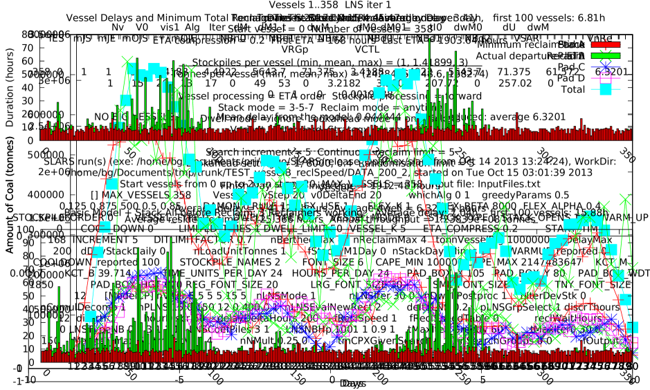
Figure 7: Vessel delay profiles in the solutions of the instance 1..358 for the basic model and basic + “stack all before reclaim” and “at most 3 reclaimers active”, obtained with the visibility horizon 15/5.

5.1 Initial solutions and solver search strategy

First we look at basic methods to obtain schedules for longer sequences of vessels. This is the EH heuristic from Section 3.4 and TTS Greedy described in Section 4, which fit into the visibility horizon schemes VH 5/5 and VH 1/1, respectively. We compare them to an approach to construct schedules in a single MiniZinc model (method “ALL”) and to the standard visibility horizon setting VH 15/5, Section 3.6. The results are given in Table 2 for the 100-vessel and 200-vessel instances. The results show some interesting properties of the solver search strategy.

Table 2: Solutions for the 100- and up to 200-vessel instances, obtained with EH, TTS, ALL, and VH 15/5.

	100 vessels								Up to 200 vessels
	EH		TTS		ALL		VH 15/5		EH		TTS		ALL		VH 15/5
1st	obj	$t$	obj	$t$	obj	$t$	obj	$t$	obj	$t$	obj	$t$	obj	$t$	obj	$t$
1	11.77	71	9.87	73	13.31	275	6.17	1509	6.15	170	5.09	90	7.06	356	3.19	1934
21	7.01	69	6.11	33	9.46	275	4.19	1758	3.75	142	3.25	68	5.08	352	2.23	2101
41	2.54	46	1.68	12	2.93	271	1.31	702	2.02	175	1.60	62	2.62	348	1.26	1465
61	0.64	42	0.61	18	0.98	273	0.51	214	3.59	252	3.25	60	5.39	351	2.63	1719
81	0.46	35	0.39	18	0.54	272	0.32	236	3.81	139	3.40	310	5.73	352	2.71	2084
101	0.33	29	0.23	7	0.52	272	0.19	202	3.39	140	3.21	62	5.14	352	1.91	2444
121	0.40	27	0.38	8	0.54	272	0.26	169	4.79	108	4.23	46	4.45	360	2.33	1815
141	2.82	154	1.44	20	2.59	273	1.35	612	4.72	220	3.26	47	4.45	353	2.45	2184
161	5.13	43	5.26	11	7.68	273	3.67	2031	3.53	101	3.26	42	5.15	352	2.25	2350
181	5.45	35	5.16	10	8.23	273	3.84	1438	3.13	70	2.93	33	4.72	328	2.17	1519
Mean	3.65	55	3.11	21	4.68	273	2.18	887	3.89	152	3.35	82	4.98	350	2.31	1961

Method “ALL”, obtaining feasible solutions for the whole 100-vessel and 200-vessel instances in a single run of the solver, became possible after a modification of the default search strategy from Section 3.3. This did not produce better results however, so we present its results only as a motivation for iterative methods for initial construction and improvement.

The default solver search strategy LayerSearch(1,…,$|V|$) proved best for the iterative methods EH and LNS. But feasible solutions of complete instances in a single model only appeared possible with a modification. The alternative strategy can be expressed as

$$\textsc{GroupLayerSearch(1,\ldots,\text{$|V|$})}=(\textsc{LayerSearch(1,\ldots,5)};\textsc{LayerSearch(6,\ldots,10)};\ \ldots)$$

which means: search for departure times of vessels $1,\ldots,5$; then for the reclaim times of their stockpiles; then for their pad numbers; …departure times of vessels $6,\ldots,10$; etc. It is similar to the iterative heuristic EH with the difference that the solver has the complete model and (presumably) takes the first found feasible solution for every 5 vessels.

We had to increase the time limit per solver call: 4 minutes. But the flattening phase took longer than finding a first solution (there are a quadratic number of constraints). Feasible solutions were found in about 1–2 minutes after flattening. We also tried running the solver for longer but this did not lead to better results: the solver enumerates near the leaves of the search tree, which is not efficient in this case. Switching to the solver’s default strategy after 300 seconds (search annotation cpx_warm_start [13]) gave better solutions, comparable with the EH heuristic.

In Table 2 we see that the solutions obtained by the “ALL” method are inferior to EH. Thus, for all further tests we used strategy LayerSearch(1,…,$|V|$) from Section 3.3. Further, EH is inferior to TTS, both in quality and running time. This proves the efficiency of the opportunity costs in TTS and suggests using TTS for initial solutions. However, TTS runs on original real-valued data and we could not use its solutions in LNS because the latter works on rounded data which usually has small constraint violations for TTS solutions. A workaround would be to use the rounded data in TTS but given the extended model implemented in MiniZinc only and the majority of running time spent in LNS, and for simplicity we stayed with EH to obtain starting solutions. The results for VH 15/5 where LNS worked on every visibility horizon, support this choice.

5.2 Visibility horizons

In this subsection, we look at the impact of varying the visibility horizon settings (Section 3.6), including the complete horizon (all vessels visible). More specifically, we compare $N=1,4,6,10,15,25$, or $\infty$ visible vessels and various numbers $F$ of vessels to be fixed after the current horizon is scheduled. For $N=\infty$, we can apply a global solution method. Using Constraint Programming, we obtain an initial solution and try to improve it by LNS, denoted by global LNS, because it operates on the whole instance. Using Adaptive Greedy (Section 4), we also operate on complete schedules.

To illustrate the behaviour of global methods, we pick the difficult instance with vessels 1..100, cf. Figure 7. A graphical illustration of the progress over time of the global methods AG(130,0) and VH 15/5 + LNS(500, 15, 12) is given in Figure 8.

Figure 8: Progress of the objective value in AG(130,0) (left) and VH 15/5 + LNS(500, 15, 12) (right), vessels 1..100

To investigate the value of various visibility horizons, for limited horizons, we applied the same settings as the standard one (Section 3.6): an initial schedule for the current horizon is obtained with EH and then improved with LNS(30, 15, 12). Results for the instance 1..100 are given in Table 4. We see that the best of the limited visibility horizon settings is VH 25/5; only the global approach, spending more time, achieves a (much) better solution. Table 4 gives the average results for all 100-vessel instances. On average, the global Constraint Programming approach (500 LNS iterations) gives the best results, but VH 25/5 is close. Moreover, the setting VH 15/1 which invests significant effort by fixing only one vessel in a horizon, is slightly better than VH 25/12, which shows that with a smaller horizon, more computational effort can be fruitful.

Table 3: Visibility horizon trade-off: vessels 1..100, basic model

N/F	1/1	4/2	6/3	10/5	15/7	15/1	25/12	25/5	15/5+GLNS
Delay, h	16.02	11.1	9.4	7.93	6.85	6.29	6.02	5.44	4.72
%$\Delta$	239%	135%	99%	68%	45%	33%	28%	15%
Time, s	194	430	481	612	2244	6542	3766	7507	10204
%$\Delta$	-98%	-96%	-95%	-94%	-78%	-36%	-63%	-26%

Table 4: Visibility horizon trade-off: all 100-vessel instances, basic model

N/F	1/1	4/2	6/3	10/5	15/7	15/1	25/12	25/5	15/5+GLNS
Delay, h	5.36	3.51	3.16	2.55	2.28	2.16	2.29	1.96	1.73
%$\Delta$	210%	103%	83%	48%	32%	25%	33%	13%
Time, s	114	188	202	267	916	2896	1823	3354	4236
%$\Delta$	-97%	-96%	-95%	-94%	-78%	-32%	-57%	-21%

The visibility horizon setting 1/1 produces the worst solutions. The TTS heuristic of Section 4 also uses this visibility horizon, but produces better results, see Tables 6 and 7. The reason is probably the more sophisticated search strategy in TTS, which minimizes ‘opportunity costs’ related to reclaimer flexibility. At present, it is impossible to implement this complex search strategy in MiniZinc, the search sublanguage would need significant extension to do so.

Table 5 reports similar results for the up to 200-vessel instances, additionally varying the number of fixed vessels in each horizon. Again, VH 25/5 is the best of tested limited horizon configurations, seconded by VH 15/1.

Table 5: Visibility horizon trade-off: averages over all the up to 200-vessel instances, basic model

N/F	1/1	4/2	6/3	10/5	15/7	25/12	15/1
Delay, h	5.77	3.49	3.25	2.66	2.30	2.16	2.15
%$\Delta$	194%	78%	66%	36%	17%	10%	10%
Time, s	337	518	518	654	1739	3656	6608
%$\Delta$	-97%	-96%	-96%	-95%	-87%	-73%	-51%
N/F		4/1	6/2	10/3	15/4	25/5	25/5 + GLNS 300
Delay, h		3.36	3.23	2.60	2.28	2.00	1.96
%$\Delta$		71%	65%	33%	16%	2%
Time, s		917	721	1211	2442	7525	13479
%$\Delta$		-93%	-95%	-91%	-82%	-44%

5.3 Comparison of Constraint Programming and Adaptive Greedy

To compare the Constraint Programming and the AG approaches, we select the following methods:

• Visibility horizon 15/5

• Visibility horizon 15/5, followed by global LNS 500

• Visibility horizon 25/5

• Visibility horizon 25/5, followed by global LNS 300

• TTS Greedy, one iteration on the ETA order

• Adaptive greedy, 500 iterations in both phases

• Adaptive greedy, 1000 iterations in Phase I only

The results for the 100-vessel instances are in Table 6, for the up to 200-vessel instances in Table 7. The pure-random configuration of the Adaptive Greedy, AG_0/1000, showed inferior performance, and its results are not given. We observe superior performance of LNS on majority of the instances.

As discussed in Section 4.2, CP approach works with discrete measures. We experimented with increasing discretization up to 10 minutes, 10 meters, and 10 tonnes. This slightly improved running times but also impaired objective values by several percent. Still, this might be more robust for real-life solutions.

Table 6: Basic model, 100 vessels: VH and LNS vs. (adaptive) greedy

	Constraint Programming							TTS Greedy and Adaptive Greedy
	VH 15/5		VH 15/5∗+G			VH 25/5		AG1		AG500/500			AG1000/0
1st	obj	$t$	obj	$t$	iter	obj	$t$	obj	$t$	obj	$t$	iter	obj	$t$	iter
1	6.17	1509	4.72	10204	338	5.44	7507	9.87	73	5.67	9992	130	5.67	7500	130
21	4.19	1758	3.17	10529	494	3.30	6626	6.11	33	3.63	10433	333	3.25	23051	991
41	1.31	702	1.24	922	0	1.24	3256	1.68	12	1.00	11253	667	1.02	12660	903
61	0.51	214	0.50	279	0	0.51	912	0.61	18	0.54	2713	126	0.54	2769	126
81	0.32	236	0.32	299	0	0.32	1266	0.39	18	0.34	11972	696	0.36	5794	344
101	0.19	202	0.19	285	2	0.18	943	0.23	7	0.21	7764	771	0.22	15	1
121	0.26	169	0.26	258	3	0.26	971	0.38	8	0.28	3589	525	0.29	201	28
141	1.35	612	0.73	4883	469	0.90	1364	1.44	20	0.80	4895	255	0.76	12969	652
161	3.67	2031	2.50	8172	369	3.51	4241	5.26	11	3.24	12574	845	3.78	4166	284
181	3.84	1438	3.64	6525	311	3.89	6450	5.16	10	3.83	6818	422	3.65	13843	809
Mean	2.18	887	1.73	4236	199	1.96	3354	3.11	21	1.95	8200	477	1.95	8297	427

^∗ For limited visibility horizons, LNS(20,12,12) was applied

Table 7: Basic model, up to 200 vessels: VH and LNS vs. (adaptive) greedy

	Constraint Programming							TTS Greedy and Adaptive Greedy
	VH 15/5		VH 25/5+G			VH 25/5		AG1		AG500/500			AG1000/0
1st	obj	$t$	obj	$t$	iter	obj	$t$	obj	$t$	obj	$t$	iter	obj	$t$	iter
1	3.19	1934	2.69	18246	274	2.82	10442	5.09	90	3.63	72884	539	3.68	102290	793
	2.23	2101	2.05	15671	243	1.79	8573	3.25	68	1.96	6496	81	1.92	72050	866
	1.26	1465	1.19	11681	286	1.15	6369	1.60	62	1.07	7461	86	1.06	7580	86
.	2.63	1719	2.37	14884	245	1.82	6728	3.25	60	2.09	38128	532	1.94	32747	442
.	2.71	2084	1.87	16147	291	2.14	8113	3.40	310	2.21	31628	252	2.04	86931	663
.	1.91	2444	1.78	12404	173	2.23	7842	3.21	62	2.04	102010	860	2.22	56555	590
	2.33	1815	1.84	14295	272	1.71	6380	4.23	46	2.08	82210	894	2.32	26512	272
	2.45	2184	1.90	12304	214	2.10	7361	3.26	47	2.17	57381	674	2.15	5451	61
	2.25	2350	1.87	12729	279	2.02	6638	3.26	42	2.12	33929	522	2.46	18109	287
181	2.17	1519	2.04	6429	12	2.20	6801	2.93	33	1.99	16687	488	1.99	16668	488
Mean	2.31	1961	1.96	13479	229	2.00	7525	3.35	82	2.14	44881	493	2.18	42489	455

5.4 Extended model

This subsection tests the extended model options from Section 3.2 with the default visibility horizon setting, Section 3.6.

A sensitivity analysis for the extended constraints is given in Table 8:

• Allowing different pads for the stockpiles of a same vessel deteriorates the solutions, similar to the results in [15]. Our experiments with the search strategy did not change this conclusion, thus we accept the “same pad” strategy as default.

• Stacking all stockpiles for a vessel before reclaiming slightly deterioated solutions, and adds some cost in producing solutions.

• The constraint of at most 3 reclaimers working simultaneously is very strong, doubling the delays, and substantially increasing solving time.

• Setting tidal weight of 80,000t (about 20% of the vessels) has almost no effect. But even 70,000t, exceeded by about 50% of the vessels, increases average delay only a little. The reason is that we update the earliest departure for delay calculation to the next tidal window border. Without doing this, the delays are much larger. The reduced choice caused by tidal constraints substantially improves solving time.

• The channel constraints are complex to model and thus costly in solving time, and do significantly extend average delay.

• Allowing 80% daily stacking volume deviation gives only a small improvement. Allowing $\pm 1$ day stacking duration reduces the delays by a factor of 3 in the basic model; but similar schedules arise if we simply shorten all stacking durations by 1 day, which is computationally simpler.

• The combined effect of the new constraints “stack all before reclaim”, “tidal weight 70,000t”, “at most 3 reclaimers”, and “channel constraints” is nearly the sum of their effects.

• In this “full” setting, reducing the stacking duration by one day has a smaller effect, but still leads to a reduction in delay of 11%.

Table 10 gives visibility horizon trage-offs with the new constraints. The percentage impacts are slightly smaller than in the basic model, Table 5.

As discussed in the end of Section 2.2, some of the first and last vessels of an instance are possibly easy to schedule because they have more resources. To investigate the hardness of processing ‘middle’ vessels, we report average delays excluding 40 ‘warm-up’ and 20 ‘cool-down’ vessels, however in solutions where still the total delay was minimized. The corresponding visibility horizon trade-offs with the new constraints are given in Table 10. As expected, the delay values are larger, cf. Table 10. The effects of the visibility horizon changes are similar to the original objective.

Table 8: Sensitivity for the new constraints

		100 vessels				Up to 200 vessels
		obj	$t$	%$\Delta$obj	%$\Delta t$	obj	$t$	%$\Delta$obj	%$\Delta t$
0)	Basic model∗	2.18	887			2.31	1961
	Diff pads	2.52	672	16%	-24%	2.52	1398	9%	-29%
1)	Stack all before	2.43	1018	11%	15%	2.43	2091	5%	7%
2)	3 reclaimers	4.78	1279	119%	44%	4.41	2612	91%	33%
	Tidal 80,000t	2.26	666	4%	-25%	2.21	1657	-4%	-16%
3)	Tidal 70,000t	2.38	705	9%	-21%	2.38	1693	3%	-14%
4)	Channel	3.14	1519	44%	71%	3.07	3303	33%	68%
80% daily stk flex		2.22	1171	2%	32%	2.27	3108	-2%	58%
	$\pm$1 day stk dur	0.82	884	-62%	0%	0.74	2679	-68%	37%
5)	$-$1 day stk dur	0.81	444	-63%	-50%	0.80	1164	-65%	-41%
	0-4)	5.80	1472	166%	66%	5.38	3343	133%	70%
	0-5)	5.14	1418	-11%	-4%	4.81	3120	-11%	-7%

^∗ The constraint on 4 berthed ships is already included by default

Table 9: Up to 200: VH trade-off with the new constraints: stack all stockpiles before reclaim; max 3 reclaimers; tidal ship weight 70’000t; channel constraint

N/F	1/1	4/2	6/3	10/5	15/7	25/12
Delay, h	11.62	7.97	6.72	5.82	5.35	5.29
%$\Delta$	141%	65%	39%	21%	11%	10%
Time, s	419	852	933	1425	2708	5123
%$\Delta$	-97%	-94%	-94%	-90%	-81%	-65%
N/F		4/1	6/2	10/3	15/4	25/5	’25/5 + GLNS 300
Delay, h		7.42	6.36	5.77	5.07	4.97	4.82
%$\Delta$		54%	32%	20%	5%	3%
Time, s		1517	1271	1910	3580	10280	14511
%$\Delta$		-90%	-91%	-87%	-75%	-29%

Table 10: Up to 200: VH trade-off with the new constraints, average delay reported under exclusion of the first 40 and last 20 vessels

N/F	1/1	4/1	6/2	10/3	15/4	25/5	’25/5 + GLNS 300
Delay, h	13.39	8.59	7.30	6.66	5.69	5.48	5.36
%$\Delta$	150%	60%	36%	24%	6%	2%

5.5 Dwell reduction.

As already noticed in [15], it is better not to reduce dwell during schedule construction. We found it better to increase dwell, in order to free resources for future vessels. Moreover, our experiments with dwell reduction for limited visibility horizons led to worse results as well.

Thus, at the moment we only reduce dwell by post-processing the complete solution. Reclaim times are fixed and we simply try to move the stacking start time of stockpiles forward as much as possible without violating stacking capacity constraints. This is done for the stockpiles of consecutive groups of 5 vessels. Average results before and after dwell post-processing are given in Table 11. Clearly the post-processing massively reduces dwell.

Table 11: Average dwell before and after dwell reduction, hours

	Basic model				Basic + 1,2,3,4)
	100 vessels		Up to 200 vessels
Mean dwell	81	6.3	78	6.6	80	7.9

An example of the effect of dwell reduction on a pad schedule is given in Figure 9.

Figure 9: Example pad schedules: before and after dwell reduction

5.6 Queue jumps

In practice, understanding the changes to the vessel processing order, as compared to the ETA order, is important: a customer which has timely arrived to the port entrance is not happy to see too many other vessels arriving later and being processed before him. We did not implement any constraints on such ‘queue jumps’ but observed them in the obtained solutions. Namely, we registered the following values:

• maximal jump (number of vessels) of a vessel behind its ETA-based position, in the vessel ordering by berth start time (arrival)

• same as above, in the ordering by berth end time (departure)

Table 12 presents the above characteristics of the CP (VH 15/5, basic model) and AG_500/500 solutions. We see that jumps by departure times are a little higher. CP solutions have larger order permutations. They increase even more after global LNS.

We may consider adding variables and constraints to directly model and constrain queue jumping in the future.

Table 12: Order jumps by arrival, departure time

	100 vessels				Up to 200 vessels
1st	CP		AG		CP		AG
1	8	11	13	13	14	15	7	9
21	11	11	7	10	13	14	7	7
41	5	5	1	4	4	8	2	4
61	2	4	3	5	11	12	8	9
81	1	4	1	4	12	16	7	8
101	1	1	1	2	14	17	5	7
121	2	4	2	4	16	17	10	10
141	5	7	2	4	16	17	5	5
161	12	13	6	6	13	14	8	8
181	10	10	8	10	11	11	5	5
mean	5.7	7.0	4.4	6.2	12.4	14.1	6.4	7.2

6 Conclusions and outlook

We consider a complex problem involving scheduling and allocation of cargo assembly in a stockyard, loading of cargoes onto vessels, and vessel scheduling. We designed a Constraint Programming (CP) approach to construct feasible solutions and improve them by Large Neighbourhood Search (LNS).

Investigation of various visibility horizon settings has shown that larger numbers of known arriving vessels lead to better results. In particular, the visibility horizon of 25 vessels provides solutions close to the best found. Among the extended model options, the strongest impacts arise from: the restriction to 3 reclaimers working at any time, which increased the average delay by 91%; and the possibility to speed up stacking by 1 day, which reduced delays by 65% in the basic model and by 11% with all the new constraints added.

We observed that the constraints involving reclaimer moving speed, (3b) and (3c), were very difficult for the solver, given that we model reclaim scheduling at a minute granularity. Simplifying the model to ignore reclaimer movement time caused the models to be much easier to solve and allowed a larger number of vessels to be considered together in one solver call. However, in the obtained solutions more than half of the necessary travel distance between reclaim jobs was to be covered in zero time, which is unacceptable.

For the basic variant of the model, the new approach was compared to an existing greedy heuristic. The latter works with a visibility horizon of one vessel and, under this setting, produces better feasible solutions in less time. The reason is probably the sophisticated search strategy which cannot be implemented in the chosen CP approach at the moment. To make the comparison fairer, an adaptive iterative scheme was proposed for this greedy heuristic, which resulted in a similar performance to LNS.

Overall the CP approach using visibility horizons and LNS generated the best overall solutions in less time than the adaptive greedy approach. A significant advantage of the CP approach is that it is easy to include additional constraints, as we have done here.

For further work, it might be important to incorporate other existing types of stockyard operation. An estimation of the solutions’ closeness to optimum is another goal. The Constraint Programming approach could benefit from integration of LNS into solver’s search strategy.

Acknowledgments

The research presented here is supported by ARC linkage grant LP110200524. We would like to thank the strategic planning team at HVCCC for many insightful and helpful suggestions, Andreas Schutt for hints on efficient modeling in MiniZinc, as well as to Opturion for providing their version of the CPX solver under an academic license.

References

- [1] Bay, M., Crama, Y., Langer, Y., Rigo, P.: Space and time allocation in a shipyard assembly hall. Annals of Operations Research 179(1), 57–76 (2010)
- [2] Beldiceanu, N., Contejean, E.: Introducing global constraints in CHIP. Mathematical and Computer Modelling 20(12), 97–123 (1994)
- [3] Belov, G., Boland, N., Savelsbergh, M.W.P., Stuckey, P.J.: Local search for a cargo assembly planning problem. In: Simonis, H. (ed.) Integration of AI and OR Techniques in Constraint Programming, Lecture Notes in Computer Science, vol. 8451, pp. 159–175. Springer International Publishing (2014)
- [4] Boland, N., Gulczynski, D., Savelsbergh, M.: A stockyard planning problem. EURO Journal on Transportation and Logistics 1(3), 197–236 (2012)
- [5] Boland, N.L., Savelsbergh, M.W.P.: Optimizing the Hunter Valley Coal Chain. In: Gurnani, H., Mehrotra, A., Ray, S. (eds.) Supply Chain Disruptions, pp. 275–302. Springer London (2012)
- [6] Clautiaux, F., Jouglet, A., Carlier, J., Moukrim, A.: A new constraint programming approach for the orthogonal packing problem. Computers & Operations Research 35(3), 944–959 (2008)
- [7] HVCCC: Hunter valley coal chain — overview presentation (2014), http://www.hvccc.com.au/
- [8] Lesh, N., Mitzenmacher, M.: BubbleSearch: A simple heuristic for improving priority-based greedy algorithms. Information Processing Letters 97(4), 161–169 (2006)
- [9] Lodi, A., Martello, S., Vigo, D.: Recent advances on two-dimensional bin packing problems. Discrete Applied Mathematics 123(1–3), 379–396 (2002)
- [10] Marriott, K., Stuckey, P.J.: A MiniZinc tutorial (2012), http://www.minizinc.org/
- [11] Ohrimenko, O., Stuckey, P.J., Codish, M.: Propagation = lazy clause generation. In: Bessière, C. (ed.) Principles and Practice of Constraint Programming — CP 2007, Lecture Notes in Computer Science, vol. 4741, pp. 544–558. Springer Berlin Heidelberg (2007)
- [12] Ohrimenko, O., Stuckey, P., Codish, M.: Propagation via lazy clause generation. Constraints 14(3), 357–391 (2009)
- [13] Opturion Pty Ltd: Opturion CPX user’s guide: version 1.0.2 (2013), www.opturion.com
- [14] Pisinger, D., Ropke, S.: Large neighborhood search. In: Gendreau, M., Potvin, J.Y. (eds.) Handbook of Metaheuristics, International Series in Operations Research & Management Science, vol. 146, pp. 399–419. Springer US (2010)
- [15] Savelsbergh, M., Smith, O.: Cargo assembly planning. EURO Journal on Transportation and Logistics pp. 1–34 (2014)
- [16] Schulte, C., Tack, G., Lagerkvist, M.Z.: Modeling and programming with Gecode (2014), www.gecode.org
- [17] Schutt, A., Feydy, T., Stuckey, P.J., Wallace, M.G.: Explaining the cumulative propagator. Constraints 16(3), 250–282 (2011)
- [18] Schutt, A., Feydy, T., Stuckey, P.J., Wallace, M.G.: Solving RCPSP/max by lazy clause generation. Journal of Scheduling 16(3), 273–289 (2013)
- [19] Schutt, A., Stuckey, P.J., Verden, A.R.: Optimal carpet cutting. In: Lee, J. (ed.) Principles and Practice of Constraint Programming — CP 2011, Lecture Notes in Computer Science, vol. 6876, pp. 69–84. Springer Berlin Heidelberg (2011)
- [20] Singh, G., Sier, D., Ernst, A.T., Gavriliouk, O., Oyston, R., Giles, T., Welgama, P.: A mixed integer programming model for long term capacity expansion planning: A case study from the hunter valley coal chain. European Journal of Operational Research 220(1), 210–224 (2012)
- [21] Thomas, A., Singh, G., Krishnamoorthy, M., Venkateswaran, J.: Distributed optimisation method for multi-resource constrained scheduling in coal supply chains. International Journal of Production Research 51(9), 2740–2759 (2013)