Spherical collapse of small masses in the ghost-free gravity

Abstract:

We discuss some properties of recently proposed models of a ghost-free gravity. For this purpose we study solutions of linearized gravitational equations in the framework of such a theory. We mainly focus on the version of the ghost-free theory with the exponential modification $\exp(\Box/\mu^{2})\Box^{-1}$ of the free propagator. The following three problems are discussed: (i) Gravitational field of a point mass; (ii) Penrose limit of a point source boosted to the speed of light; and (iii) Spherical gravitational collapse of null fluid. For the first problem we demonstrate that it can be solved by using the method of heat kernels and obtain a solution in a spacetime with arbitrary number of dimensions. For the second problem we also find the corresponding gyraton-type solutions of the ghost-free gravitational equations for any number of dimensions. For the third problem we obtain solutions for the gravitational field for the collapse of both ”thin” and ”thick” spherical null shells. We demonstrate how the ghost-free modification of the gravitational equations regularize the solutions of the linearized Einstein equations and smooth out their singularities.

1 Introduction

It is widely believed that the quantum gravity will ”cure” a decease of the classical general relativity, its singularities. In particular, in the domain of a spacetime near singularities, where the curvature becomes large, the Einstein equations should be modified. Such a modification, which, for example, is dictated by the string theory, should include additional terms in the gravitational effective action, that are both, higher in curvature and in its derivatives. It was proposed many different modifications of the Einstein theory of the general relativity, that, in particular, change its infrared and ultraviolet behavior (see, e.g. a review [1]). In this paper we discuss a special class of the modified gravity theory with higher derivatives. It is instructive to check at first the effects of such a modification in the linearized version of the corresponding theory. It is well known that addition of quadratic in the curvature corrections modifies the standard Laplace equation for the gravitational potential $\varphi$ in the Newtonian approximation, which takes, for example, the following form

$$(l^{2}\bigtriangleup+1)\bigtriangleup\varphi=4\pi\rho\,.$$ (1)

It is easy to show that such a modified equation for a point mass has a decreasing at the infinity solution, which remains finite at $r=0$. The parameter $l$, which is determined by the coupling constant for the quadratic in the curvature term in the effective action, provides a UV cut-off in the regularized solution (see e.g. [2, 3]). A general analysis of the Newtonian singularities in higher derivative gravity models was recently performed in [4].

A connected problem is a possibility of mini-black hole production in the gravitational collapse of a small mass. To study such a problem one may consider it first in the linearized version of the theory. If a corresponding solution is regular and its curvature for a small mass $M$ is uniformly small in the whole spacetime, one might conclude that in this regime higher in curvature corrections are small and can be neglected. In such a case one can expect that for the small enough mass $M$ a black hole is not formed. In other words, in such a theory there exists a mass gap for the back hole formation. Long time ago in the paper [3] it was demonstrated that the gravitational theory with quadratic in the curvature terms in the action possesses this property.

However, in a general case, a propagator in a theory with higher derivatives contains extra poles, reflecting the existence of the additional to the gravitons degrees of freedom. As a result, the corresponding theory with higher derivatives usually contains ghosts [2, 5, 6]. In order to avoid this problem a new type of the modification of the Einstein theory, called ghost-free gravity, was proposed [7, 8, 9, 10, 11]. A similar model was proposed earlier in [12] (for general discussion see [13, 14]).

The main idea of this approach is to consider a theory, which is non-local in derivatives. Suppose that in the linearized version of such a theory the box operator $\Box$ is modified and takes the form $a(\Box)\,\Box$, where $a(z)$ is an entire function of the complex variable $z$. Then the propagator for such a theory does not have additional poles, different from the original pole, describing propagation of the gravitons. There exists a variety of entire functions. It is sufficient to use the function $a(z)$ to be an exponent of the polynomial in $z$. The simplest choice is when this polynomial is a linear function, so that the modified box-operator is $\exp(-\Box/\mu^{2})\Box$, where $\mu$, which has the dimensionality of the mass, is the UV cut-off parameter. One may hope that such cut-off regularizes singularities inside black holes [15, 16] and in the big-bang cosmology [17, 18, 19, 20, 16]. It should be emphasized that non-local operators of a similar form and their properties were considered long time ago in the papers [21, 22, 23, 24, 25, 26].

In the present paper we study solutions of the ghost-free gravitational equations in the linearized approximation. In the section 2 we demonstrate that for any number of spacetime dimensions $D$ a solution for the Newtonian potential for a point mass can be obtained by using the heat kernel method. We describe these solutions and compare them with the solutions of the linearized Einstein equations. We demonstrate that for $D\geq 4$ the gravitational potential is regular at the position of the source, and the parameter $\mu$ is the scale of the UV regularization. We also show that for $D=4$ the obtained result coincides with the one obtained earlier by the Fourier method and presented in the paper [7]. In section 3 we boost the solution for a static point mass. By taking the Penrose limit with $v\to c$ of the boosted metric, we obtain a solution of the ghost-free equations for gravitational field of a ”photon” moving in $D$-dimensional spacetime. We show that these solutions are similar to the field of non-rotating gyratons [27, 28, 29]. The main difference is that a function of $(D-2)$ transverse variables, which enters the metric of the gyraton and which is a solution of the $(D-2)$ flat Laplace equation, in the ghost-free gravity becomes a solution of the $(D-2)$ operator $a(-\bigtriangleup)\bigtriangleup$. As a result, the singularity of the gyraton metric at its origin is smooth. In the next sections 4–5 we study the problem of the spherical collapse of null fluid in the ghost-free gravity. In section 4 we demonstrate how a solution for the spherical null shell collapse can be obtained as a superposition of a spherical distribution of gyratons, that pass through the fixed point and are the generators of the null shell. The method can be used in a spacetime with an arbitrary number of dimensions. In the present paper we illustrate it for a special case of the four dimensional spacetime. We use this approach to obtain a solution for the gravitational field of a thin null shell in the ghost-free theory. We show that a solution, obtained in the developed gyraton-based approach, correctly reproduces the known solution for the collapsing null shell in the linearized Einstein gravity. We obtain also a solution for the ghost-free gravity and compare it with the solution for the Einstein gravity. In particular, we calculate the Kretschmann curvature invariant for the solution and demonstrate that its singularity is smoothened. However, it remains divergent at the origin $r=0$. Finally, we study the collapse of a spherical thick null shell and obtain its gravitational field by taking a specially chosen superposition of thin null shells (section 5). We demonstrate that the ghost-free gravitational field is everywhere regular in this model, and for small mass $M$ the apparent horizon (and hence a black hole) does not form. This means that in the ghost-free gravity there is a mass gap for the mini black hole formation in the gravitational collapse, and, in this sense, its properties are somehow similar to the properties of the theory with quadratic in curvature corrections, discussed in [3]. Section 6 contains summary and discussions of the obtained results. Appendices contain details of the derivation of the thin null shell metric from the gyraton solutions. In this paper we use the sign convention adopted in the book [30].

2 Non-local Newtonian gravity

2.1 Newtonian potential in the ghost-free gravity

In this paper we consider solutions of the linearized ghost-free gravity equations. We start by analyzing static solutions for a point mass in this approximation. Such a solution gives a modified Newtonian potential. The gravitational field of a point source in four dimensions was obtained earlier in [7, 15]. The authors of these papers used the Fourier method for this purpose. We demonstrate that this result can be obtained much easier by using the method of the heat kernels. This method, practically without any changes, allows one to solve a similar problem in the higher dimensional case. We consider a flat spacetime and denote by $D$ the number of its dimensions. It is often convenient to use a number $n$, connected with $D$ as follows $D=n+3$. The static metric in the weak-field approximation in the standard $D$ dimensional gravity can be written in the form (see e.g. [29])

$$ds^{2}=-(1+2\varphi)dt^{2}+\left(1-{2\over n}\varphi\right)d\ell^{2}\,,\hskip 5.69046ptd\ell^{2}=\delta_{ij}dx^{i}dx^{j}\,,\hskip 5.69046pti,j=1,\ldots,D-1\,,$$ (2)

where the Newtonian potential $\varphi$ satisfies the equation

$$\bigtriangleup\varphi=4\pi G\rho\,,\hskip 14.22636ptG={2n\over n+1}G^{D}\,.$$ (3)

The operator $\bigtriangleup$ is a standard $(D-1)$-dimensional Laplace operator, which in the flat (Cartesian) coordinates is of the form

$$\bigtriangleup(\ldots)=\delta^{ij}(\ldots)_{,ij}\,.$$ (4)

In the four-dimensional spacetime $n=1$, so that $G=G^{4}$ and (3) takes the standard form of the Poisson equation for the Newtonian gravitational potential. It should be emphasized that there exists an ambiguity in the choice of the form of the higher dimensional coupling constant. We denote this constant by $G^{D}$ and fixed it by the requirement that the form of the Einstein equation is the same in any number of dimensions

$$S[g]={1\over 16\pi G^{D}}\int d^{D}x\sqrt{-g}R\,.$$ (5)

We introduce another constant $G$, related with $G^{D}$ in such a way, that the form of the equation for the Newtonian potential $\varphi$ is the same for any $D$. For a point mass $m$

$$\rho=m\delta^{n+2}(x)\,,$$ (6)

and the potential $\varphi$ is (see e.g. [29])

$$\varphi=-{2\Gamma(1+n/2)\over\pi^{n/2}n}{Gm\over r^{n}}\,.$$ (7)

In the four-dimensional case this expression takes the standard form $\varphi=-Gm/r$.

Following [7] we write the modified ghost-free equation for the Newtonian gravitational potential $\tilde{\varphi}$, created by a point source of the mass $m$, in the form

$$\hat{F}\tilde{\varphi}=4\pi G\rho\,,\hskip 14.22636pt\hat{F}=a(\bigtriangleup)\bigtriangleup\,.$$ (8)

We shall use the following form of the non-local operator $a(\bigtriangleup)$, proposed in [7]

$$a(\bigtriangleup)=e^{-\bigtriangleup/\mu^{2}}\,.$$ (9)

The parameter $\mu$ specifies the characteristic energy scale, where the adopted theory modification becomes important. In what follows we shall also use another parameter, $s$, related with $\mu$ as follows

$$s=\mu^{-2}\,.$$ (10)

This is convenient, since some of the relations will contain derivatives and integrals over $s$, which do not look ”elegant” in terms of $\mu$. On the other hand, $\mu$ has more direct ”physical meaning” as the mass (energy) of the UV cut-off of the modified gravity. After required calculations are performed one can simply substitute the parameter $s$ in terms of $\mu$ by using the relation (10).

2.2 Heat kernel approach

Let us discuss now equation (8) and its solution. We shall use the following standard notions. For any operator $\hat{B}$ we denote by $B(x,x^{\prime})$ its value in the $x$-representation

$$B(x,x^{\prime})=\langle x|\hat{B}|x^{\prime}\rangle\,.$$ (11)

In these notations $\delta$-function is

$$\delta(x,x^{\prime})=\langle x|\hat{I}|x^{\prime}\rangle\,,$$ (12)

where $\hat{I}$ is a unit operator. Using these notations one can write the equation (8) as follows

$$\int dx^{\prime}\,F(x,x^{\prime})\tilde{\varphi}(x^{\prime})=4\pi G\rho(x)\,.$$ (13)

We denote by $\hat{A}$ an inverse to $\hat{F}$ operator

$$\hat{A}=\hat{F}^{-1}={1\over\bigtriangleup}e^{s\bigtriangleup}=e^{s\bigtriangleup}{1\over\bigtriangleup}\,.$$ (14)

We denote

$$\hat{D}=-{1\over\bigtriangleup}\,,\hskip 14.22636pt\hat{K}(s)=e^{s\bigtriangleup}\,,$$ (15)

so that relation (14) takes the form

$$\hat{A}=-\hat{D}\hat{K}(s)=-\hat{K}(s)\hat{D}\,.$$ (16)

In the $x$-representation $D(x,x^{\prime})$ is nothing but a usual Green function of the Laplace operator and it obeys the equation

$$\bigtriangleup\hat{D}=-\hat{I}\,.$$ (17)

The other operator, $\hat{K}(s)$, is also well known. In $x$-representation it is just a standard heat kernel $K_{n}(x,x^{\prime}|s)$ of the Laplace operator. It has the following form

$$K_{n}(x,x^{\prime}|s)\equiv{1\over(4\pi s)^{1+n/2}}e^{-\lambda(x,x^{\prime})/(4s)}\,.$$ (18)

This formula requires some explanations. We remind that we denoted by $D=n+3$ the total number of spacetime dimensions. Since the gravitational field of a static source is static, the gravitational potential depends only on $D-1=n+2$ spatial coordinates. Correspondingly, the heat kernel (18) is a function of 2 spatial points, $x$ and $x^{\prime}$ and $\lambda(x,x^{\prime})$ is the square of the spatial distance between these points

$$\lambda(x,x^{\prime})=|x-x^{\prime}|^{2}\,.$$ (19)

The degree $1+n/2$ of expression in the denominator reflects the fact that we are working in a space with $D-1=n+2$ dimensions.

It is easy to check that the operator $\hat{A}$ can be written in terms of $\hat{K}(s)$ as follows

$$\hat{A}_{n}=-\int_{s}^{\infty}ds\,\hat{K}_{n}(s)\,.$$ (20)

Relations (18) and (20) allow one to obtain a solution of the equation (8)-(9). For a point mass $m$ at point $x^{\prime}=0$ one has

$$\tilde{\varphi}(x)=4\pi mA_{n}(x,0)=-4\pi Gm\int_{s}^{\infty}ds\,\hat{K}_{n}(x,0|s)\,.$$ (21)

Before presenting explicit form of the solutions for the Newtonian potential $\tilde{\varphi}$ in the ghost-free gravity, let us make the following remark. The equations (8)–(9) can be identically rewritten in the form

$$\bigtriangleup\tilde{\varphi}=4\pi G\tilde{\rho}\,,\hskip 14.22636pt\tilde{\rho}=\hat{K}_{n}(s)\rho\,.$$ (22)

In other words, the Newtonian potential $\tilde{\varphi}$ in the ghost-free gravity is a solution of the standard Poisson equation for the source $\tilde{\rho}$, which is obtained by smearing the original distribution $\rho(x)$. For the point mass (6) the smeared source is

$$\tilde{\rho}(x)=mK_{n}(x,0|s)\,.$$ (23)

In this approach one may say that the ghost-free gravity regularizes the potential $\tilde{\varphi}$ by smearing a source, which generates it. Of course, the results obtained by the source smearing and by applying $\hat{A}$ operator to ”un-smeared” source $\rho$ are the same. Let us present the results.

In flat three-dimensional space $(D=4,n=1)$ in Cartesian coordinates

$$K_{1}(x,x^{\prime}|s)={1\over(4\pi s)^{3/2}}e^{-{\lambda\over 4s}}\,,$$ (24)

$$A_{1}(x,x^{\prime})=-{1\over 4\pi\sqrt{\lambda}}\mbox{erf}\left({\sqrt{\lambda}\over 2\sqrt{s}}\right)\,,$$ (25)

$$\tilde{\varphi}=-{Gm\over r}\mbox{erf}\left({\mu r\over 2}\right)\,.$$ (26)

Here $\mbox{erf}(x)$ is the Gauss error function, which is defined as follows

$$\mbox{erf}(x)={2\over\sqrt{\pi}}\int_{0}^{x}\,e^{-t^{2}}dt\,.$$ (27)

Formula (26) correctly reproduces the expression for the gravitational potential in the linearized ghost-free gravity, obtained earlier [7, 15].

In flat four-dimensional space $(D=5,n=2)$ in Cartesian coordinates

$$K_{2}(x,x^{\prime}|s)={1\over(4\pi s)^{2}}e^{-{\lambda\over 4s}}\,,$$ (28)

$$A_{2}(x,x^{\prime})=-{1\over 4\pi^{2}\lambda}\left[1-e^{-\lambda/(4s)}\right]\,,$$ (29)

$$\tilde{\varphi}=-{Gm\over\pi r^{2}}\left(1-\exp(-\mu^{2}r^{2}/4)\right)\,.$$ (30)

There exist simple relations between $K_{n}(x,x^{\prime}|s)$ and $A_{n}(x,x^{\prime})$ in spacetimes with different number of dimensions

$$K_{n+2}(x,x^{\prime}|s)={1\over\pi}{\partial\over\partial\lambda}K_{n}(x,x^{\prime}|s)\,,\hskip 5.69046ptA_{n+2}={1\over\pi}{\partial\over\partial\lambda}\,A_{n}(x,x^{\prime})\,.$$ (31)

Using these relations one can obtain a general expression for $A_{n}(x,x^{\prime})$

$$A_{n}(x,x^{\prime})=-{\gamma\left({n/2},{\lambda/(4s)}\right)\over 4\pi^{(n+1)/2}\lambda^{n/2}}\,,\hskip 14.22636ptn\geq 2\,.$$ (32)

This relation contains a so called lower incomplete gamma function $\gamma(a,x)$, which is is defined as

$$\gamma(a,x)=\int_{0}^{x}\ t^{a-1}e^{-t}dt=x^{a}\Gamma(a)e^{-x}\sum_{k=0}^{\infty}{x^{k}\over\Gamma(a+k+1)}\,.$$ (33)

Thus in the ghost-free gravity the Newtonian field of a point mass $m$ is

$$\tilde{\varphi}(r)=-Gm{\gamma\left({n/2},{r^{2}/(4s)}\right)\over\pi^{(n-1)/2}r^{n}}\,.$$ (34)

At small $x$ one has $\gamma(a,x)\approx x^{a}/a$. Hence

$$\tilde{\varphi}(r=0)=-{2Gm\over n\pi^{(n-1)/2}(4s)^{n/2}}\,.$$ (35)

This relation implies that the Newtonian potential of a point mass in the ghost-free gravity in any number of dimensions $D\geq 4$ is finite at the origin. In other words, this potential is properly regularized.

3 Non-spinning gyratons in the ghost-free gravity

We obtain now the gravitational field of an ultra-relativistic particle in the framework of the ghost-free gravity. Instead of solving the modified gravitational equations for a source moving with the speed of light we use the following procedure which is well known in the standard General Relativity. We first make the Lorentz transformation of the static solution for a point mass $m$ and obtain the metric for the object moving with velocity $\beta$. After this we take a so called Penrose limit of the metric of the moving body. Namely, we take the limit $\beta\to 1$, while keeping the energy of the object $\gamma m$ fixed. As a result one obtains an object in $D$-dimensional spacetime which was called a gyraton [27, 28, 29]. In a general case, when a static source has an angular momentum, the corresponding gyraton is spinning. We restrict ourselves by the case of non-spinning gyratons. A new element in our derivation is performing the described procedure not within the General Relativity, but in the ghost-free theory of gravity.

To perform the calculations it is convenient to use the following notations for the standard Cartesian coordinates $x^{\mu}=(\bar{t},y,{\mbox{\boldmath$\zeta$}}_{{\scriptscriptstyle\perp}})$. Here $\bar{t}$ is just the time in the frame, where the source is at rest, $y$ is the coordinate in the direction of motion of the source, and ${\mbox{\boldmath$\zeta$}}_{{\scriptscriptstyle\perp}}=(\zeta^{2},\ldots,\zeta^{D-2})$ are the coordinates in $(D-2)$ dimensional plane orthogonal to the direction of the motion. We shall call the latter the transverse coordinates. The Newtonian potential for a point source of mass $m$ in the ghost-free gravity, obtained in the previous section, takes the following form in these coordinates

$$ds^{2} = ds_{0}^{2}+dh^{2}\,,$$ (36)

$$ds_{0}^{2} = -d\bar{t}^{2}+dy^{2}+d\zeta_{{\scriptscriptstyle\perp}}^{2}\,,\hskip 14.22636ptd\zeta_{{\scriptscriptstyle\perp}}^{2}=\sum_{2}^{n+1}(d\zeta_{i})^{2}\,,$$ (37)

$$dh^{2} = -2\tilde{\varphi}\left[d\bar{t}^{2}+{1\over n}(dy^{2}+d\zeta_{{\scriptscriptstyle\perp}}^{2})\right]\,,$$ (38)

where $\tilde{\varphi}$ is defined by (34).

To obtain a metric for a source moving with the velocity $\beta$ (along the $y$-axis in the positive direction) we make the following Lorentz transformation

$$\begin{split}y&=\gamma(\xi-\beta t)={\gamma\over 2}[(1-\beta)v-(1+\beta)u]\,,\\ \bar{t}&=\gamma(t-\beta\xi)={\gamma\over 2}[(1-\beta)v+(1+\beta)u]\,.\end{split}$$ (39)

Here $(t,\xi,{\mbox{\boldmath$\zeta$}}_{{\scriptscriptstyle\perp}})$ are Cartesian coordinates in the new inertial frame, where the source is moving. We also denoted

$$\gamma=(1-\beta^{2})^{-1/2}\,,\hskip 5.69046ptu=t-\xi\,,\hskip 5.69046ptv=t+\xi\,.$$ (40)

The flat metric $ds_{0}^{2}$ in the new coordinates $x^{\mu}=(u,v,{\mbox{\boldmath$\zeta$}}_{{\scriptscriptstyle\perp}})$ is

$$ds_{0}^{2}=-du\,dv+d\zeta_{{\scriptscriptstyle\perp}}^{2}\,.$$ (41)

The form of this metric remains the same in the limit $\beta\to 1$, while in this limit

$$y\sim-\gamma u\,,\hskip 14.22636pt\bar{t}\sim\gamma u\,,\hskip 14.22636pt\lambda(x,0)\sim\gamma^{2}u^{2}+\zeta_{{\scriptscriptstyle\perp}}^{2}\,,$$ (42)

$$d\bar{t}^{2}+{1\over n}(dy^{2}+d\zeta_{{\scriptscriptstyle\perp}}^{2})\sim{n+1\over n}\gamma^{2}du^{2}+\ldots\,.$$ (43)

Here $\ldots$ denote sub-leading in $\gamma$ terms. As a result, the metric perturbation in this limit takes the form

$$dh^{2}=\Phi du^{2}\,,\hskip 14.22636pt\Phi=-{2(n+1)\over n}\lim_{\gamma\to\infty}(\gamma^{2}\tilde{\varphi})\,.$$ (44)

When taking this limit, we assume, as usual, that the energy of the object, $\gamma m$ is fixed (the Penrose limit), and we denote

$$M=G\gamma m\,.$$ (45)

We also use the following relation

$$\lim_{\gamma\to\infty}\gamma e^{-{\gamma^{2}u^{2}\over 4s}}=\sqrt{4\pi s}\delta(u)\,.$$ (46)

Combining these results, we finally obtain the following expression for the function $\Phi$

$$\Phi=-8\pi{n+1\over n}M\delta(u)A_{n-1}(\zeta_{{\scriptscriptstyle\perp}})\,,$$ (47)

where

$$A_{n-1}(\zeta_{{\scriptscriptstyle\perp}})=-\int_{s}^{\infty}{ds\over(4\pi s)^{{n+1\over 2}}}\,e^{-\zeta_{{\scriptscriptstyle\perp}}^{2}/(4s)}\,.$$ (48)

Let us notice, that $A_{n-1}(\zeta_{{\scriptscriptstyle\perp}})$ is nothing, but a solution of the ghost-free gravity equations for a point source, reduced to $D-2$ dimensional transverse plane with coordinates ${\mbox{\boldmath$\zeta$}}_{{\scriptscriptstyle\perp}}$. For large $\mu$ it reduces to a solution of the $D-2$ dimensional Poisson equations. This means, that in this limit the obtained solution of the ghost-free gravity equations reduces to the standard metric of non-rotating gyratons [27, 28, 29].

In what follows we restrict ourselves by considering a four dimensional spacetime. For this case the integral, which enters the definition of $A_{0}$, has an infrared divergence at large $s$. Let us discuss this case in more detail. Let us notice that

$$A_{0}=-{1\over 4\pi}\int_{s}^{\eta^{2}}{ds\over s}e^{-\zeta_{{\scriptscriptstyle\perp}}^{2}/(4s)}={1\over 4\pi}\left[\mbox{Ei}(1,\zeta_{{\scriptscriptstyle\perp}}^{2}/(4s)+\mbox{Ei}(1,\zeta_{{\scriptscriptstyle\perp}}^{2}/(4\eta^{2})\right]\,.$$ (49)

The parameter $\eta$, which has the dimensionality of the length, is an infra-red cut-off parameter. Here $\mbox{Ei}(a,z)$ is the exponential integral defined as

$$\mbox{Ei}(a,z)=\int_{1}^{\infty}dx\,x^{-a}\,e^{-xz}\,.$$ (50)

The function $\mbox{Ei}(1,z)$ for small $z$ has the following expansion

$$\mbox{Ei}(1,z)=-\ln(z)-\gamma+\ldots\,.$$ (51)

Here $\gamma=0.5772156649$ is the Euler constant, and $\ldots$ denote the terms vanishing in the $z=0$ limit. Assuming that $\eta^{2}$ is large and using (51) one can write

$$A_{0}={1\over 4\pi}\left[\ln(\zeta_{{\scriptscriptstyle\perp}}^{2}/\eta^{2})+\gamma+\mbox{Ei}(1,\zeta_{{\scriptscriptstyle\perp}}^{2}/(4s)\right]\,.$$ (52)

The corresponding expression for the metric is

$$ds^{2}=-dudv+d\zeta_{{\scriptscriptstyle\perp}}^{2}+dh^{2}\,,\hskip 14.22636ptdh^{2}=\Phi du^{2}\,,$$ (53)

$$\Phi=-4M\delta(u)F(\zeta_{{\scriptscriptstyle\perp}}^{2})\,,$$ (54)

$$F(\zeta_{{\scriptscriptstyle\perp}}^{2})=\ln(\zeta_{{\scriptscriptstyle\perp}}^{2}/\eta^{2})+\gamma+\mbox{Ei}(1,\zeta_{{\scriptscriptstyle\perp}}^{2}/(4s))\,.$$ (55)

In the limit $\mu\to\infty$, when the ghost-free gravity reduces to the Einstein theory,

$$F(\zeta_{{\scriptscriptstyle\perp}}^{2})=\ln(\zeta_{{\scriptscriptstyle\perp}}^{2}/\eta^{2})+\gamma\,.$$ (56)

This result reproduces the well known Aichelburg-Sexl solution [31] (see also [32]).

Let us notice that the solution (55) contains an arbitrary parameter, the infrared cut-off parameter $\eta$. However, the change of this parameter can be easily absorbed into the redefinition of the advanced time $v$. Hence, this ambiguity just reflects freedom in the gauge choice. In order to demonstrate this, let us consider a metric of the form

$$ds^{2}=-dudv+d\zeta_{{\scriptscriptstyle\perp}}^{2}+f(u)du^{2}\,.$$ (57)

Let us define a new coordinate

$$\bar{v}=v-\int duf(u)\,.$$ (58)

Then one gets

$$ds^{2}=-dud\bar{v}+d\zeta_{{\scriptscriptstyle\perp}}^{2}\,.$$ (59)

This confirms our above conclusion, that the ambiguity in the choice of the cut-off parameter $\eta$ can always been absorbed in the change of the coordinates. In what follows we use this option and simply put $\eta^{2}=4s$. For this choice

$$F(z)=\ln(z)+\gamma+\mbox{Ei}(1,z)\,,\hskip 14.22636ptz=\zeta_{{\scriptscriptstyle\perp}}^{2}/(4s)\,.$$ (60)

For this choice the expansion of the function $F(z)$ for small $z$ takes a very simple form

$$F(z)=z-{1\over 4}z^{2}+O(z^{3})\,.$$ (61)

4 Null shell collapse

4.1 Null shell as a superposition of null gyratons

We use now the above described gyraton metric in order to study the gravitational collapse in the ghost-free gravity. Namely, we consider a collapse of a spherical null shell. As earlier we use linearized gravitational equations. For simplicity, we restrict ourselves by 4D case. Instead of solving the corresponding equations we shall use the following trick. Let us notice that a sum of solutions of the linearized theory is again a solution. In the linear approximation the solution has the form

$$ds^{2}=ds_{0}^{2}+dh^{2}\,.$$ (62)

Here $ds_{0}^{2}$ is the flat metric and $dh^{2}$ is a perturbation.

Let us consider a set of gyratons passing through a chosen point $O$ of the spacetime. We use the Cartesian coordinates $(t,X,Y,Z)$ in the the Minkowski spacetime, and identify a point $O$ with the origin of the coordinate system $O=(0,0,0,0)$. We denote by $({\mbox{\boldmath$e$}}_{{\scriptscriptstyle X}},{\mbox{\boldmath$e$}}_{{\scriptscriptstyle Y}},{\mbox{\boldmath$e$}}_{{\scriptscriptstyle Z}})$ unit vectors in the directions of the axes $X$, $Y$, and $Z$, respectively, and by $n$ a unit vector in 3D space in the direction of the motion of a fixed gyraton. One has

$${\mbox{\boldmath$n$}}=\sin\alpha\,(\cos\beta~{}{\mbox{\boldmath$e$}}_{{\scriptscriptstyle X}}+\sin\beta~{}{\mbox{\boldmath$e$}}_{{\scriptscriptstyle Y}})+\cos\alpha~{}{\mbox{\boldmath$e$}}_{{\scriptscriptstyle Z}}\,.$$ (63)

Here $(\alpha,\beta)$ are standard coordinates on a unit 2D sphere. Let $a$ be an index enumerating the gyratons and the metric perturbation created by such a gyraton is $dh_{a}^{2}$. Then the perturbation $\langle dh^{2}\rangle$ created by a set of the gyratons has the form

$$\langle dh^{2}\rangle=\sum_{a}dh_{a}^{2}\,.$$ (64)

We assume that all gyratons have the same energy. We also take a continuous limit of the discrete distribution of the gyratons and assume that such a distribution is spherically symmetric. Thus, we write

$$\langle dh^{2}\rangle={1\over 4\pi}\int_{0}^{\pi}d\alpha\,\sin\alpha\int_{0}^{2\pi}d\beta\ \ dh^{2}_{(\alpha,\beta)}\,.$$ (65)

An extra factor $(4\pi)^{-1}$ reflects that we use averaging over a unit sphere.

As a result of the averaging, the source of the metric $dh^{2}$ is a thin null shell located at the null cones $\Gamma_{\pm}$

$$t=\pm\sqrt{X^{2}+Y^{2}+Z^{2}}\,.$$ (66)

For the sign minus, $\Gamma_{-}$ is a null cone with apex at $O$, which describes a collapsing spherical null shell. For the sign plus, the null cone $\Gamma_{+}$ describes an expanding null shell. Our starting point is gyraton metric (53), which we rewrite in the form

$$ds_{0}^{2}=-dt^{2}+d\xi^{2}+d\zeta_{{\scriptscriptstyle\perp}}^{2}\,,\hskip 14.22636ptdh^{2}=\Phi(dt-d\xi)^{2}\,,\hskip 14.22636pt\Phi=-4MF(\zeta_{{\scriptscriptstyle\perp}}^{2})\delta(t-\xi)\,.$$ (67)

Here

$$F=\left\{\begin{array}[]{ll}\displaystyle{\ln(\zeta_{{\scriptscriptstyle\perp}}^{2}/\eta^{2})\,,}&\mbox{for the Einstein theory}\,;\\ \displaystyle{\mbox{Ei}(1,\zeta_{{\scriptscriptstyle\perp}}^{2}/4s)+\gamma+\ln(\zeta_{{\scriptscriptstyle\perp}}^{2}/4s)\,,}&\mbox{for the ghost-free gravity}\,.\end{array}\right.$$ (68)

Let us notice that this is a metric of a gyraton without spin. Namely these gyratons will be considered in this paper. We also found convenient to use the following terminology. We call a worldline of a gyraton a null string. Its projection to the 3D space, the gyraton trajectory, is an oriented straight line. A unit orientation vector $n$ along this line determines a direction of the motion. Quantity $\xi$ is the coordinate along the trajectory in the direction of motion of the ”photon”, and $\zeta_{{\scriptscriptstyle\perp}}=(\zeta_{1},\zeta_{2})$ are Cartesian coordinates in the 2D plane orthogonal to this direction. We study a spherically symmetric distribution of the gyratons, which has the property that the null strings, representing them, intersect at a single spacetime point $O$. We also choose the parameter $\xi$ along each of the strings to vanish at this point $O$. Consider a point $P=(X,Y,Z)$ of the 3D space. There exist exactly two gyraton trajectories, passing through this point. Let $(\alpha_{+},\beta_{+})$ be angles of a unit vector ${\mbox{\boldmath$n$}}_{+}$ (see (63)) along the line, connecting the origin with the point $P$. The parameter $\xi_{+}$ at $P$ for such a trajectory is positive. The direction vector for the second trajectory is ${\mbox{\boldmath$n$}}_{-}=-{\mbox{\boldmath$n$}}_{+}$ and its angles are $(\alpha_{-}=\pi-\alpha_{+},\beta_{-}=\pi+\beta_{+})$, while the corresponding coordinate $\xi_{-}=-\xi_{+}$ is negative.

It is convenient to perform the calculations of $\langle dh^{2}\rangle$ in two steps. First we introduce the following objects

$$T^{(\alpha,\beta)}(y_{{\scriptscriptstyle\perp}})=\delta^{2}(y_{{\scriptscriptstyle\perp}}-\zeta_{{\scriptscriptstyle\perp}})\delta(t-\xi)(dt-d\xi)^{2}\,,$$ (69)

$$\langle T(y_{{\scriptscriptstyle\perp}})\rangle={1\over 4\pi}\int_{0}^{\pi}d\alpha\sin\alpha\int_{0}^{2\pi}d\beta\ \ T^{(\alpha,\beta)}(y_{{\scriptscriptstyle\perp}})\,.$$ (70)

For $y_{{\scriptscriptstyle\perp}}=0$

$$T^{(\alpha,\beta)}=T_{\mu\nu}^{(\alpha,\beta)}dx^{\mu}dx^{\nu}$$ (71)

is the stress-energy tensor of a gyraton moving in the direction $n$ (see (63)). Similarly, for $y_{{\scriptscriptstyle\perp}}=0$

$$M\langle T\rangle=T_{\mu\nu}dx^{\mu}dx^{\nu}\,,$$ (72)

where $T_{\mu\nu}$ is the stress-energy tensor of a spherical null shell, constructed from gyraton null strings. Next, we use $\langle T(y_{{\scriptscriptstyle\perp}})\rangle$ to find the metric perturbation $\langle dh^{2}\rangle$ for the thin null shell of mass $M$

$$\langle dh^{2}\rangle=M\int dy_{{\scriptscriptstyle\perp}}F(y_{{\scriptscriptstyle\perp}}^{2})\langle T(y_{{\scriptscriptstyle\perp}})\rangle\,.$$ (73)

It should be emphasized that the quantities $dh^{2}_{(\alpha,\beta)}$ and $T^{(\alpha,\beta)}(y_{{\scriptscriptstyle\perp}})$, which enter (65) and (70), must be first written in the coordinate system, that does not depend on the particular value of the parameters $(\alpha,\beta)$. We use the Cartesian coordinates $(X,Y,Z)$ for this purpose. Thus we need first to establish relations between the gyraton associated coordinates $(\xi,\zeta_{{\scriptscriptstyle\perp}})$ and the Cartesian coordinates $(X,Y,Z)$. This problem is solved in the appendix A. After this we need to calculate the integral over the sphere, which enters relation (70) for the average value $\langle T(y_{{\scriptscriptstyle\perp}})\rangle$. The details of these calculations are collected in appendix B.

4.2 Stress-energy tensor

The relation (183) can be used to find the stress-energy tensor of the null shell constructed from null strings representing a set of gyratons. Using (70) and (183) one gets

$$\langle T(y_{{\scriptscriptstyle\perp}})\rangle={1\over 4\pi|Q\xi|}\left[\sin\alpha_{+}\,\delta(t-\xi_{+})\,(dt-d\xi_{+})^{2}+\sin\alpha_{-}\,\delta(t-\xi_{-})\,(dt-d\xi_{-})^{2}\right]_{y_{{\scriptscriptstyle\perp}}}\,.$$ (74)

Taking the limit $y_{{\scriptscriptstyle\perp}}\to 0$ in this relation and using relations (72) and (179) one obtains

$$M\langle T\rangle=T_{\mu\nu}dx^{\mu}dx^{\nu}={M\over 4\pi r^{2}}[\delta(u)du^{2}+\delta(v)dv^{2}]\,,$$ (75)

where $u=t-r$, $v=t+r$. This relation correctly reproduces the expected expression for the stress-energy tensor of the null shell. It is a superposition of the stress-energy tensors of contracting and expanding spherical null shells of mass $M$. One can easily solve the linearized Einstein equations for such a null-shell problem. The solution is well known and simple. Inside both the collapsing and expanding shells the spacetime is flat, while outside them the metric is a linearized version of the Schwarzschild metric

$$\langle dh^{2}\rangle={2M\over r}(dt^{2}+dr^{2})\,.$$ (76)

Our next goal is to reproduce this result by using the representation (73). This will provide us with a useful test of the validity of our approach.

4.3 Averaged metric

We have all the required expressions to perform the calculations. However, one can greatly simplify the problem using the following observation. Since the distribution of the null strings representing gyratons is spherically symmetric, the corresponding averaged metric $\langle dh^{2}\rangle$ must also have this property. Hence, it can be written in the form

$$\langle dh^{2}\rangle=h_{tt}dt^{2}+2h_{tr}dtdr+h_{rr}dr^{2}+Hd\omega^{2}\,.$$ (77)

Here the metric coefficients $h_{tt}$, $h_{tr}$, $h_{rr}$ and $H$ are functions of $t$ and $r$, and $d\omega^{2}$ is the metric on a unit sphere. The spherical coordinates $(r,\theta,\phi)$ are related with the Cartesian coordinates $(X,Y,Z)$ as follows

$$X=r\sin\theta\cos\phi\,,\hskip 14.22636ptY=r\sin\theta\sin\phi\,,\hskip 14.22636ptZ=r\cos\theta\,.$$ (78)

In order to find the metric (77) it is sufficient to obtain its value near a single spatial point. We choose such a point as follows: $P_{{\scriptscriptstyle X}}=(X=r,0,0)$, where $X>0$. For this choice the metric (77) reduces to

$$\langle dh^{2}\rangle=h_{tt}dt^{2}+2h_{tr}dtdX+h_{rr}dX^{2}+{H\over r^{2}}\,\left(dY^{2}+dZ^{2}\right)\,.$$ (79)

We perform now calculations of $\langle dh^{2}\rangle$ at $P_{X}$ and by comparing it with (79) we find the expression for the metric perturbation (77). One has near $P_{{\scriptscriptstyle X}}$

$$Q_{\pm}=\pm\sqrt{X^{2}-y_{p}^{2}}\,,\hskip 14.22636pt\xi_{\pm}=\pm\sqrt{X^{2}-y_{{\scriptscriptstyle\perp}}^{2}}\,,$$ (80)

$$\sin\alpha_{\pm}={\xi_{\pm}\over Q_{\pm}}\,,\hskip 14.22636pt\cos\alpha_{\pm}=-{y_{k}\over Q_{\pm}}\,,$$ (81)

$$\sin\beta_{\pm}={y_{p}\over X}\,,\hskip 14.22636pt\cos\beta_{\pm}={Q_{\pm}\over X}\,,$$ (82)

$$d\xi_{\pm}={\xi_{\pm}\over X}dX+{1\over Q_{\pm}}\left(\xi_{\pm}\,{y_{p}\over X}\,dY-y_{k}\,dZ\right)\,.$$ (83)

In order to obtain the metric perturbation $\langle dh^{2}\rangle$ one must to calculate the integral over $(y_{p},y_{k})$ in (73). We introduce polar coordinates in the $(y_{p},y_{k})$-plane:

$$y_{p}=\rho\cos\psi\,,\hskip 14.22636pty_{k}=\rho\sin\psi\,.$$ (84)

We also write

$$\langle T(y_{{\scriptscriptstyle\perp}})\rangle=T^{+}+T^{-}\,,$$ (85)

$$T^{\pm}={1\over 4\pi Q^{2}}\,\delta(t-\xi_{\pm})\,(dt-d\xi_{\pm})^{2}\,.$$ (86)

Because of the presence of $\delta$-function the term $T^{+}$ is non-zero only for $t\geq 0$, while the other term $T^{-}$ is non-zero for $t\leq 0$. We write expression (73) in the form

$$\langle dh^{2}\rangle=-4M\int_{0}^{\infty}d\rho\rho F(\rho^{2})({\cal T}^{+}+{\cal T}^{-})\,,$$ (87)

$${\cal T}^{\pm}=\int_{0}^{2\pi}d\psi T^{\pm}\,.$$ (88)

One has

$$(dt-d\xi_{\pm})^{2}=A_{\pm}+{B_{\pm}\over Q^{2}}+\ldots\,,\hskip 14.22636ptQ^{2}=X^{2}-\rho^{2}\cos^{2}\psi\,,$$ (89)

$$A_{\pm}=(dt-{\xi_{\pm}\over X}dX)^{2}\,,\hskip 14.22636ptB_{\pm}=(a_{\pm}\cos\psi+b\sin\psi)^{2}\,,$$ (90)

$$a_{\pm}={\xi_{\pm}\rho dY\over X}\,,\hskip 14.22636ptb=-\rho dZ\,,$$ (91)

and dots indicate terms linear in $y_{p}$ and $y_{k}$, which do not contribute to the integral over $\psi$ (88). Thus one has

$${\cal T}^{\pm}={\delta(t-\xi_{\pm})\over 4\pi}\,(A_{\pm}\,K_{1}+K_{2})\,,\hskip 5.69046ptK_{1}=\int_{0}^{2\pi}{d\psi\over Q^{2}}\,,\hskip 5.69046ptK_{2}=\int_{0}^{2\pi}{d\psi\,B_{\pm}\over Q^{4}}\,.$$ (92)

Integrals $K_{1}$ and $K_{2}$ can be easily taken with the following result

$$K_{1} = {2\pi\over X\sqrt{X^{2}-\rho^{2}}}\,,$$ (93)

$$K_{2} = {\pi[(a_{\pm}^{2}+b^{2})X^{2}-b^{2}\rho^{2}]\over X^{3}(X^{2}-\rho^{2})^{3/2}}={\pi\rho^{2}\over X^{3}\sqrt{X^{2}-\rho^{2}}}(dY^{2}+dZ^{2})\,.$$ (94)

$\delta$-function in (92) can be written as

$$\delta(t\mp\sqrt{X^{2}-\rho^{2}})={|t|\over\rho}\delta(\rho-\sqrt{X^{2}-t^{2}})\,.$$ (95)

This relation also implies that

$$t=\pm\sqrt{X^{2}-\rho^{2}}\,.$$ (96)

After integration in (87) the terms ${\cal T}^{\pm}$ give similar contributions, so that finally one obtains the following result

$$\langle dh^{2}\rangle={-2MF(X^{2}-t^{2})\over X}\left[\left(dt-{t\over X}dX\right)^{2}+{X^{2}-t^{2}\over 2X^{2}}(dY^{2}+dZ^{2})\right]\,.$$ (97)

Comparing (97) with (79) we finally get

$$\langle dh^{2}\rangle={-2MF(r^{2}-t^{2})\over r}\left[\left(dt-{t\over r}dr\right)^{2}+{r^{2}-t^{2}\over 2}d\omega^{2}\right]\,.$$ (98)

This expression is valid everywhere in the domain $r\geq|t|$ for both positive and negative time $t$.

Using GRTensor program one can check that the Ricci tensor for this perturbation of the flat metric in the linear in $M$ approximation vanishes everywhere outside the null shell. This provides one with a good test of the correctness of the performed calculations.

4.4 A case of linearized Einstein equations

For the linearized Einstein equations

$$F(r^{2}-t^{2})=\ln\left({r^{2}-t^{2}\over\eta^{2}}\right)\,.$$ (99)

The corresponding expression (98) looks quite different from the expected answer (76). However one can use the gauge freedom

$$h_{\mu\nu}\to h_{\mu\nu}-V_{(\mu;\nu)}\,,$$ (100)

to transform (98) into the expected form. It is sufficient to choose

$$V_{\mu}=(V_{t},V_{r},0,0)\,,$$ (101)

$$V_{t}=-{2Mt\over r}(1+t/r)\ln\left({r^{2}-t^{2}\over\eta^{2}}\right)+2M\ln{r-t\over r+t}+{2Mt\over r}\,,$$ (102)

$$V_{r}=-{M\over r^{2}}(r^{2}-t^{2})\ln\left({r^{2}-t^{2}\over\eta^{2}}\right)\,.$$ (103)

After this gauge transformation one gets

$$\langle dh^{2}\rangle={2M\over r}(dt^{2}+dr^{2})\,.$$ (104)

Let us notice that the infrared cut-off $\eta^{2}$ in (99) does not enter the final result and the change of this parameter is simply absorbed into the redefinition of the gauge field $V_{\mu}$. Let us mention also that the Kretschmann invariant

$${\cal R}^{2}=R_{\mu\nu\alpha\beta}R^{\mu\nu\alpha\beta}$$ (105)

in its lowest non-vanishing order is

$${\cal R}^{2}={48M^{2}\over r^{6}}\,,$$ (106)

as it must be for the Schwarzschild metric. Let us emphasize that the same result can be obtained directly from the perturbation of the metric in the form (98).

4.5 Ghost-free case

One can easily repeat similar calculations for the an arbitrary function $F(z)$, where where $z=r^{2}-t^{2}$. We used the GRTensor program for this purpose. The calculations are straightforward. However, the intermediate formulas are quite long. That is why we do not reproduce them here. Let us only present the expression for the Kretschmann invariant in its lowest order for such the metric in the ghost-free gravity

$${\cal R}^{2}={48M^{2}z^{2}\over r^{6}}Q(z)\,,\hskip 5.69046ptQ(z)=2{{\cal F}^{\prime}}^{2}z^{2}+2{\cal F}{{\cal F}^{\prime}}z+{\cal F}^{2}\,,\hskip 5.69046pt{\cal F}=F^{\prime}\,.$$ (107)

For the ghost-free theory with $a(\Box)=\exp(-\Box/\mu^{2})$ one has

$$F(z) = Ei(1,z/(4s))+\gamma+\ln(z/(4s))\,,$$ (108)

$${\cal F}(z) = {1\over z}\left(1-e^{-z/4s}\right)\,,$$ (109)

$$Q(z) = {1\over 8s^{2}z^{2}}\left((8s^{2}+4sz+z^{2})e^{-z/2s}-4s(4s+z)e^{-z/4s}+8s^{2}\right)\,.$$ (110)

Using the expansion (61) of $F$ for small $z$

$$F(z)={z\over 4s}-{z^{2}\over 64s^{2}}+\ldots\,.$$ (111)

one finds

$${\cal R}^{2}={3M^{2}z^{2}\over s^{2}r^{6}}+\ldots={3M^{2}\beta^{2}\over s^{2}r^{4}}+\ldots\,.$$ (112)

Here $\beta^{2}=1-t^{2}/r^{2}$ is a dimensionless parameter which outside the shell, where $|t|<r$, is less or equal to 1. This means that the curvature for the linearized ghost-free theory in a case of the collapse of the spherical null shell is weaker than the singularity for the linearized Einstein equations. However, the ghost-free gravity solution still remains singular at least for the chosen scheme of the regularization.

5 Spherical ”thick” null shell collapse: Results

5.1 ”Thick” null shell model

In the previous section we discussed the gravitational field of a spherical null thin shell. This shell represents a spherical $\delta$-type distribution of the energy. The mass of the shell is $M$. It collapses with the speed of light and shrinks to zero radius at the moment of time $t=0$. In the linearized theory the corresponding perturbation of the background flat metric is $\langle dh^{2}\rangle(t,r)$. Certainly, such a model is an idealization. To study more realistic model of the collapse we assume that the spherical collapsing null fluid is represented by a pulse, which is not infinitely sharp in time, but has final time duration. We characterize its profile by a function $q(t)$. The meaning of this function is the mass density per a unit time, $dM/dt$, arriving to the center $r=0$ at time $t$. The total mass of such ”thick” shell is

$$M=\int dt\ q(t)\,.$$ (113)

Using the linearity of the equations one can write the corresponding solution $\langle\!\langle dh^{2}\rangle\!\rangle(t,r)$ as the superposition of $\langle dh^{2}\rangle(t,r)$ perturbations as follows

$$\langle\!\langle dh^{2}\rangle\!\rangle(t,r)=\int dt^{\prime}q(t^{\prime})\langle dh^{2}\rangle(t-t^{\prime},r)\,.$$ (114)

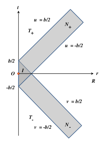
Figure 1: Thick null shell collapse

To simplify the calculations we further specify the model. Namely, we choose $q(t)$ to be a step function, which has a constant value $M/b$ during the interval $t\in(-b/2,b/2)$, and which vanishes outside this interval. For such a step function a solution has different form in the different spacetime domains (see Figure 1). Let us describe first these domains. It is convenient to use the advanced time, $v=t+r$, and the retarded time, $u=t-r$, coordinates. In the domains $T_{-}$, where $v<-b/2$, and $T_{+}$, where $u>b/2$, the spacetime is empty, and the metric is flat there. In the domain $N_{-}$, where $v\in(-b/2,b/2)$ and $u<-b/2$, one has only in-falling null fluid flux, while in $N_{+}$, where $u\in(-b/2,b/2)$ and $v>b/2$ one has only out-going null fluid flux. In the domain, $I$, where $v\in(-b/2,b/2)$ and $u\in(-b/2,b/2)$ one has a superposition of the in-coming and out-going null fluid fluxes. And finally, in the domain $R$, where $v>b/2$ and $u<-b/2$, the spacetime is empty.

5.2 Gravitational field in the $I$-domain

Let us consider first $I$-domain. Denote by $(t,r)$ the coordinates of the point of ”observation” in this domain. A thin null shell, crossing the center $r=0$ at time $t^{\prime}$, contributes to the integral (114) only if $t^{\prime}\in(t-r,t+r)$. Let us denote $x=t^{\prime}-t$, then the formula (114) takes the form

$$\langle\!\langle dh^{2}\rangle\!\rangle(t,r)=-{2M\over br}\int_{-r}^{r}dxH(r,x)\,,$$ (115)

$$H(r,x)=F(r^{2}-x^{2})\left(dt^{2}-2{x\over r}drdt+{x^{2}\over r^{2}}dr^{2}+{1\over 2}(r^{2}-x^{2})d\omega^{2}\right)\,.$$ (116)

Thus one has

$$\langle\!\langle dh^{2}\rangle\!\rangle(t,r)=-{2M\over br}\left[J_{0}(dt^{2}+{1\over 2}r^{2}d\omega^{2})+J_{2}({dr^{2}\over r^{2}}-{1\over 2}d\omega^{2})\right]\,.$$ (117)

Here

$$J_{n}=\int_{-r}^{r}dx\ x^{n}\ F(r^{2}-x^{2})\,.$$ (118)

The linear in $x$ term in (149) disappears as a result of the integration.

5.2.1 Linearized Einstein theory

For this case

$$F(z)=\ln z+C\,,\hskip 14.22636ptC=-\ln\eta^{2}\,,$$ (119)

$$J_{0}=4r(\ln 2+\ln r-1)+2Cr\,,$$ (120)

$$J_{2}={4\over 9}r^{3}(3\ln 2+3\ln r-4)+{2\over 3}Cr^{3}\,.$$ (121)

Calculations give

$${\cal R}^{2}={252\dot{M}^{2}\over r^{4}}\,,\hskip 14.22636pt\dot{M}=M/b\,.$$ (122)

5.2.2 Ghost-free gravity case

One has

$$F(z)=\mbox{Ei}(1,z/4s)+\gamma+\ln(z/4s)\,.$$ (123)

The Tailor expansion of this function for small $z$ is

$$F(z)={z\over 4s}-{z^{2}\over 64s^{2}}+{z^{2}\over 1152s^{3}}+\ldots\,.$$ (124)

Using this expansion one gets for small $r$ in the $I$-domain

$$J_{0} = {r^{3}(420s^{2}-21sr^{2}+r^{4})\over 1260s^{3}}+\ldots\,,$$ (125)

$$J_{2} = {r^{5}(756s^{2}-27sr^{2}+r^{4})\over 11340s^{3}}+\ldots\,$$ (126)

Calculations of the Kretschmann invariant ${\cal R}^{2}$ for small $r$ in the $I$-domain give

$${\cal R}^{2}={32\dot{M}^{2}\over 3s^{2}}-{32\dot{M}^{2}r^{2}\over 9s^{3}}+\ldots\,.$$ (127)

Here, as earlier, $\dot{M}=M/b$. This relation shows that for the thick shell model the curvature remains finite at $r=0$.

5.2.3 $(\nabla r)^{2}$ invariant

There exists another useful invariant for the spherically symmetric geometry. This invariant is

$$(\nabla r)^{2}={1\over 4f}g^{\mu\nu}f_{,\mu}f_{,\nu}\,,\hskip 14.22636ptf=g_{\theta\theta}\,.$$ (128)

A line in the $(t,r)$ plane, where this invariant vanishes, is an apparent horizon. Using GRTensor one find that in the leading order in $M$ this invariant in the $I$-domain is

$$(\nabla r)^{2}=1-{2Mr^{2}\over sb}+\ldots\,.$$ (129)

Since in this domain $r<b$, one has

$$(\nabla r)^{2}>1-{2Mb\over s}\,.$$ (130)

This relation means that for given $s$, which is the square of the UV cut-off parameter $\mu$ of the ghost-free theory, $s=\mu^{-2}$, and fixed duration $b$ of the pulse the mini-black hole is not formed if the mass $M$ is small enough.

5.3 Gravitational field in the $R$ domain

The perturbation of the gravitational field in the $R$ domain is described by the following expression

$$\langle\!\langle dh^{2}\rangle\!\rangle(t,r)=-{2M\over br}\left[J_{0}(dt^{2}+{1\over 2}r^{2}d\omega^{2})-J_{1}{2dt\ dr\over r}+J_{2}({dr^{2}\over r^{2}}-{1\over 2}d\omega^{2})\right]\,,$$ (131)

where now

$$J_{n}=\int_{t-b/2}^{t+b/2}dx\ x^{n}\ F(r^{2}-x^{2})\,.$$ (132)

Here

$$F(z)=F_{0}(z)+\Delta F(z)\,,\hskip 5.69046ptF_{0}(z)=\gamma+\ln(z/4s)\,,$$ (133)

$$\Delta F(z)=\mbox{Ei}(1,z/4s)\,.$$ (134)

We denote by $J^{0}_{n}$ and $\Delta J_{n}$ the contribution to $J_{n}$ of the terms $F_{0}$ and $\Delta F$, respectively, so that one has

$$J_{n}=J^{0}_{n}+\Delta J_{n}\,.$$ (135)

We consider the perturbed metric at large $r$ in the $R$ domain. We also assume that $r\gg|t\pm b/2|$ and use the following asymptotic form of the function $\Delta F(z)$ for large $z$

$$\Delta F(z)={4s\over z}e^{-z/4s}(1+O(1/z))\,.$$ (136)

Thus one can use the following approximation

$$\Delta F(r^{2}-x^{2})\approx f(r)k(x)\,,\hskip 5.69046ptf(r)={1\over r^{2}}e^{-r^{2}/(4s)}\,,\hskip 5.69046ptk(x)=4se^{x^{2}/(4s)}\,.$$ (137)

Using this approximation and (132) one obtains

$$\Delta J_{n}=f(r)A_{n}(t)\,,\hskip 5.69046ptA_{n}(t)=(4s)^{{n+2\over 2}}\int_{C_{-}}^{C_{+}}dy\,y^{n}\,e^{y^{2}}\,,\hskip 5.69046ptC_{\pm}={t\pm b/2\over 2\sqrt{s}}\,.$$ (138)

Calculation of $J_{n}^{0}$ is straightforward and $J^{0}_{n}$ can be easily obtained by using the Maple program. One also obtains the following expressions for $A_{n}(t)$

$$A_{0}(t)=-4is^{3/2}\sqrt{\pi}\left(\mbox{erf}(i\tau_{+})+\mbox{erf}(i\tau_{-})\right)\,,$$ (139)

$$A_{1}(t)=8s^{2}\left(e^{\tau_{+}^{2}}-e^{\tau_{-}^{2}}\right)\,,$$ (140)

$$A_{3}(t)=4s^{2}\left[2i\sqrt{\pi s}\left(\mbox{erf}(i\tau_{+})+\mbox{erf}(i\tau_{-})\right)+(2t+b)e^{\tau_{+}^{2}}-(2t-b)e^{\tau_{-}^{2}}\right]\,.$$ (141)

Here

$$\tau_{\pm}={\pm 2t+b\over 4\sqrt{s}}\,,$$ (142)

and erf is the Error function, which is defined as

$$\mbox{erf}(x)={2\over\sqrt{\pi}}\int_{0}^{x}dt\exp(-t^{2})\,.$$ (143)

Let us emphasize that in spite of the presence of the imaginary unit $i$ in the above formulas, expressions for $A_{n}(t)$ are real, as they should be. After straightforward calculations by using the GRTensor program, we obtain the following expression for the Kretschmann tensor in the leading $M^{2}$ order

$${\cal R}^{2}={48M^{2}\over r^{6}}+\Delta{\cal R}^{2}\,,\hskip 14.22636pt\Delta{\cal R}^{2}={2M^{2}\over s^{2}br^{10}}\ e^{-r^{2}/(4s)}\,W\,,$$ (144)

$$W=-3A_{0}r^{6}+(4\ddot{A}_{0}s^{2}+8\dot{A}_{1}s-34A_{0}s+A_{2})r^{4}$$

$$+(80\dot{A}_{1}s^{2}-12\ddot{A}_{2}s^{2}-160A_{0}s^{2}+14A_{2}s)r^{2}+56A_{2}s^{2}\,.$$ (145)

Keeping the first term in $W$, which contains the highest power of $r$, we obtain

$$\Delta{\cal R}^{2}\sim{24i\sqrt{\pi}M^{2}\over\sqrt{s}br^{4}}\ e^{-r^{2}/(4s)}\,\left(\mbox{erf}(i\tau_{+})+\mbox{erf}(i\tau_{-})\right)\,.$$ (146)

Once again, in spite of the presence of $i$ the answer for $\Delta{\cal R}^{2}$ is real.

Expressions (144) and (146) imply that in the $R$ domain for a fixed value of time $t$ and $r\to\infty$ the curvature exponentially fast reaches its asymptotic value, which is equal to the Schwarzschild curvature of a spherical object of mass $M$.

5.4 Gravitational field in the $N_{\pm}$-domains

Let us briefly discuss now the gravitational field in the $N_{\pm}$ domains. We focus on the incoming $N_{-}$ domains. The case of the $N_{+}$ is similar. Let $(t,r)$ be coordinates of the ”observation” point. We denote $v=t+r$ and $u=t-r$. The condition that the ”observation” point is in the $N_{-}$ domain reads

$$v\in(-b/2,b/2)\,,\hskip 14.22636ptu\in(-\infty,-b/2)\,.$$ (147)

The position $t^{\prime}$ of the apex of the null-shells, that give non-zero contribution at the point of the ”observation”, obeys the conditions $t^{\prime}\in(-b/2,t+r)$. As earlier, we denote $x=t-t^{\prime}$. Then

$$\langle\!\langle dh^{2}\rangle\!\rangle(t,r)=-{2M\over br}\int_{-r}^{t+b/2}dxH(r,x)\,,$$ (148)

$$H(r,x)=F(r^{2}-x^{2})\left((dt-{x\over r}dr)^{2}+{1\over 2}(r^{2}-x^{2})d\omega^{2}\right)\,.$$ (149)

Thus one has

$$\langle\!\langle dh^{2}\rangle\!\rangle(t,r)=-{2M\over br}\left[J_{0}(dt^{2}+{1\over 2}r^{2}d\omega^{2})-J_{1}{2dt\ dr\over r}+J_{2}({dr^{2}\over r^{2}}-{1\over 2}d\omega^{2})\right]\,.$$ (150)

Here

$$J_{n}=\int_{-r}^{t+b/2}dx\ x^{n}\ F(r^{2}-x^{2})\,.$$ (151)

In the linearized Einstein gravity one uses the following expression for $F$

$$F(r^{2}-t^{2})=\ln\left({r^{2}-t^{2}\over\eta^{2}}\right)\,.$$ (152)

The required integrals (132) can be easily calculated. We do not reproduce here these results since the obtained expressions are quite long. We present here only final expression for the Kretschmann tensor, which we obtained by using th GRTensor program

$${\cal R}^{2}={48M^{2}(v)\over r^{6}}\,,\hskip 14.22636ptM(v)=\dot{M}(v+b/2)\,.$$ (153)

This is an expected result. Indeed, before the collapsing null fluid meets the outgoing flux, that is in the $N_{-}$-domain, one has simply the Vaidya solution with mass $M(v)={M\over b}(v+b/2)$, where $v\in(-b/2,b/2)$. For a chosen model $M(v)$ linearly grows from zero (at $v=-b/2$) till its maximal value $M$. Calculations for the metric perturbation in the $N_{+}$ are similar and give the following result

$${\cal R}^{2}={48M^{2}(u)\over r^{6}}\,,\hskip 14.22636ptM(u)=\dot{M}(u+b/2)\,.$$ (154)

In the case of the ghost-free gravity the curvature is modified in the narrow ”skin” domains close to $v=\pm b/2$ (for $N_{-}$ domain) and close to $u=\pm b/2$ (for $N_{+}$ domain), while outside of them and at large $r$ the ghost-free theory corrections only slightly modify the above described Vaidya metric.

6 Summary and discussion

Let us summarize and discuss the obtained results. We remind that we study the modification of the solutions of the Einstein theory in the framework of the ghost-free theory, proposed in [7, 8, 10, 11]. We focus mainly on a special type of such a theory in which a free field operator $\Box$ is replaced by the non-local operator of the form $\exp(-\Box/\mu^{2})\,\Box$. We study solutions of such a theory in the linearized approximation. We first study a gravitational field of a point mass in this theory. Such a problem was solved in the four dimensional space time in [7, 15] by using the Fourier methods. We demonstrate that the propagator of the linearized ghost-free theory in any number of spacetime dimensions is directly related to the heat kernel in this space. Using the heat kernel approach we obtain solutions for the gravitational field of a point mass in $D$-dimensional spacetime. We demonstrate that these solutions are always regular at the position of the source. In $4D$ spacetime the obtained solution coincides with the result presented in [7, 15].

In the second part of the paper we study solutions of the ghost-free gravity for ultra-relativistic sources. We first obtain ghost-free analogues of gyraton solutions [27, 28, 29] in the ghost-free gravity. For this purpose we boost the obtained ghost-free solution for a point mass, and by taking the Penrose limit, we found a solution for a $D$-dimensional spinless “photon”. We demonstrate that the corresponding metric is similar to the metric of a spinless gyraton. The main difference is that a solution of $(D-2)$-dimensional flat Laplace equation for a point charge, that enters the gyraton metric, is modified. Namely, the function of the transverse variables becomes a solution of $(D-2)$ ghost-free modification of the corresponding Laplace operator. Using this result we obtain spinless gyraton solutions of the ghost-free gravity in $D$-dimensional spacetime and demonstrate that their transverse singularities are regularized.

Finally, we study a spherical gravitational collapse of null fluid in the framework of the ghost-free gravity. As earlier, we restrict ourselves by working in the linearized approximation. Since a solution of the ghost-free equations for the dynamical problem seems to be complicated, we used the following trick based on the results, obtained earlier in this paper. We used a fact that in the linearized theory a superposition of any solutions is again a solution. To obtain the gravitational field for a collapsing spherical thin null, we ”construct” it as a superposition of the gyraton metrics for a spherically symmetric distribution of the gyraton sources moving along a null cone, representing the shell. Such gyratons intersect at a single point of the spacetime, which is an apex of the null cone. In the adopted linearized approximation the gyratons, forming the thin shell, cross this point simultaneously without interaction, so that after passing the apex point they form an expanding spherical null shell. The gravitational field for such null shells is obtained by averaging of the single gyraton metric over homogeneous spherical distribution of the gyratons. We demonstrated that by using this approach one correctly reproduces the stress-energy tensor for both, collapsing and expanding thin null shells. We checked that the obtained solution in the linearized Einstein gravity correctly reproduces the expected result. Namely, the gravitational field inside both, collapsing and expanding shells vanishes, while outside of them it is time independent. The latter field is nothing but a linearized version of the Schwarzschild metric with mass $M$. After this, we obtained a similar solution for the ghost-free gravity. To study its properties we calculated the Kretschmann scalar for it and demonstrated that its singularity at $r=0$ is smoothened, but still is present.

The model of an infinitely thin null shell is certainly an idealization. One can expect that in a consistent theory the non-locality cannot be a property of the gravitational field only, but similar non-locality must be present in the description of matter and other fields. For this reason a “physical” collapsing shell must have natural finite thickness, which may regularize the curvature singularity of the thin shell. In order to check this assumption, we study a case of the thick null shell collapse. In the linearized theory a corresponding solution is obtained by a superposition of the thin-shell solutions, that is by averaging these solutions with different positions of their apexes at $r=0$. As a result, we construct a solution for a thick null shell with an arbitrary distribution of the collapsing mass $M=M(v)$ at the spatial infinity. We considered in detail a special model, where the mass $M(v)$ is a linear function of the advanced time $v=t+r$, such that $\dot{M}$ vanishes for the moments $v<-b/2$ and $v>b/2$, and remains constant inside this interval. We demonstrated, that in the linearized Einstein gravity the solution is a superposition of two linearized Vaidya metrics, for the incoming and outgoing null fluid fluxes. The corresponding Kretschmann scalar is ${\cal R}^{2}={252\dot{M}^{2}\over r^{4}}$, where $\dot{M}=M/b$. It is singular at $r=0$.

In the linearized ghost-free gravity the corresponding solution is modified. The main new feature is, that the metric is regular at $r=0$. As a result, its Kretschmann scalar ${\cal R}^{2}={32\dot{M}^{2}\over 3s^{2}}$ is finite at $r=0$. We also calculated the invariant $(\nabla r)^{2}$ and demonstrated for the collapse of a thick null shell of the small mass $M$ the apparent horizon is not formed. This result can be interpreted as follows: in the ghost-free gravity there exists a mass gap for the black hole formation in the gravitational collapse. This result is similar to the result obtained in [3] for the null shell collapse in the theory gravity with quadratic in the curvature corrections. Recently it was demonstrated that the mass gap for mini black hole formation is a common property not only of the ghost-free gravity, but also of a wide class of higher derivative theories of gravity [33]. These theories contain a mass scale parameter $\mu$, which plays the role of the ultra-violet cut-off. As a result, if the mass $M$ of a collapsing object obeys the relation $M\mu\lesssim 1$, an apparent horizon is not formed. The presence of such a scale parameter, differs these theories from the classical Einstein gravity, where the mass gap is absent and the black-holes of arbitrary small mass can be formed. A well known consequence of this is Choptuik [34] type universal scaling properties of near-critical solutions.

Let us make a few general remarks concerning solutions of the ghost-free gravity equations. The heat kernels, which we used to construct solutions for a static source, are well defined in the space with the Euclidean metric. The reason is that the Laplace operator is non-positive definite. However this property is not valid for the box operator. In this paper we used the method based on the gyraton solutions to overcome this problem for a special case of the null shell collapse. It would be interesting to investigate solutions of the linearized ghost-free gravity with the form-factor $a=\exp(-\Box/\mu^{2})$ for arbitrary moving sources, say, for the emission of the gravitational waves in such a theory, and the back-reaction of this radiation on the accelerated objects. Another proposed option is to modify this form-factor, and instead of $\Box$ to consider higher powers of this operator in the exponent. A simplest example is $a=\exp(\alpha\Box^{2})$. It will be interesting to study such modifications.

In the present paper we study solutions of the linearized equations of the ghost free theory. Let us emphasize, that this is sufficient for demonstration of the existence of the mass gap for mini black hole formation in the adopted model. The reason is that if such a solution for small mass $M$ is regular and the corresponding perturbation of the flat metric is uniformly small, then one can expect that the higher order corrections to this solution can be neglected. A natural question is what happens in the collapse of large mass $M$, that is when $M\mu\gg 1$. It would be highly interesting to analyze solutions of the ghost-free gravity in this regime [15, 16]. It is natural to assume that curvature remains finite inside the black holes and the limiting curvature conjecture is satisfied [35, 36, 37]. These was a lot of discussions of non-singular models of black holes. One of the option is that the apparent horizon is closed [3] (see also [38, 39, 40] and references therein). Another option is a new universe formation inside a black hole [41, 42]. This option was also widely discussed in the literature. One may hope that proposed ghost free modifications of the Einstein gravity, which are ultraviolet complete and asymptotically free, would allow one to answer intriguing questions concerting the structure of the black hole interior.

Appendix A Useful geometric relations

In order to find this coordinate transformation let us introduce a couple of new useful unit vectors. The first one is a vector $k$ which is orthogonal to $n$ and is directed from the gyraton trajectory to the $Z$-axis (see Figure 2). It can be written as a linear combination

$${\mbox{\boldmath$k$}}=k_{{\scriptscriptstyle Z}}{\mbox{\boldmath$e$}}_{{\scriptscriptstyle Z}}+k_{{\scriptscriptstyle n}}{\mbox{\boldmath$n$}}\,.$$ (155)

Using relation $({\mbox{\boldmath$n$}},{\mbox{\boldmath$e$}}_{{\scriptscriptstyle Z}})=\cos\alpha$ one finds

$${\mbox{\boldmath$k$}}={1\over\sin\alpha}({\mbox{\boldmath$e$}}_{{\scriptscriptstyle Z}}-\cos\alpha{\mbox{\boldmath$n$}})\,.$$ (156)

The second unit vector $p$ is orthogonal to both $n$ and $k$. It can be written as

$${\mbox{\boldmath$p$}}=[{\mbox{\boldmath$n$}}\times{\mbox{\boldmath$k$}}]={1\over\sin\alpha}[{\mbox{\boldmath$n$}}\times{\mbox{\boldmath$e$}}_{{\scriptscriptstyle Z}}]\,.$$ (157)

Hence this vector is orthogonal to ${\mbox{\boldmath$e$}}_{{\scriptscriptstyle Z}}$ and lies in the $X-Y$-plane. It is easy to check that

$${\mbox{\boldmath$p$}}=\sin\beta\,{\mbox{\boldmath$e$}}_{{\scriptscriptstyle X}}-\cos\beta\,{\mbox{\boldmath$e$}}_{{\scriptscriptstyle Y}}\,.$$ (158)

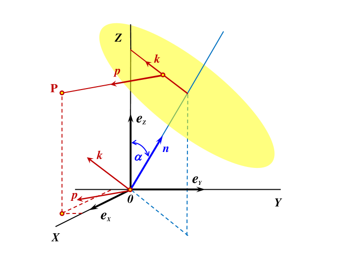
Figure 2: Relation between the Cartesian and the gyraton based coordinates

Consider a point $P$, which has the Cartesian coordinates $(X,Y,Z)$, so that the vector $P$ connecting the origin point $O$ with $P$ is

$${\mbox{\boldmath$P$}}=X{\mbox{\boldmath$e$}}_{{\scriptscriptstyle X}}+Y{\mbox{\boldmath$e$}}_{{\scriptscriptstyle Y}}+Z{\mbox{\boldmath$e$}}_{{\scriptscriptstyle Z}}\,.$$ (159)

The same vector can be written in the gyraton’s frame as follows ($\zeta_{{\scriptscriptstyle\perp}}=(\zeta_{k},\zeta_{p})$)

$${\mbox{\boldmath$P$}}=\xi{\mbox{\boldmath$n$}}+\zeta_{k}{\mbox{\boldmath$k$}}+\zeta_{p}{\mbox{\boldmath$p$}}\,.$$ (160)

By comparing (159) and (160) and using relations (63), (156) and (158) one finds

$$X = \cos\beta\,(\xi\sin\alpha-\zeta_{k}\cos\alpha)+\zeta_{p}\,\sin\beta\,,$$

$$Y = \sin\beta\,(\xi\sin\alpha-\zeta_{k}\cos\alpha)-\zeta_{p}\,\cos\beta\,,$$ (161)

$$Z = \xi\,\cos\alpha+\zeta_{k}\,\sin\alpha\,.$$

We shall also use the following inverse relations

$$\xi = \sin\alpha\,(\cos\beta X+\sin\beta Y)+\cos\alpha\,Z\,,$$ (162)

$$\zeta_{k} = -\cos\alpha\,(\cos\beta X+\sin\beta Y)+\sin\alpha\,Z\,,$$ (163)

$$\zeta_{p} = \sin\beta\,X-\cos\beta\,Y\,.$$ (164)

Using these results it is easy to show that

$$d\xi^{2}+d\zeta_{{\scriptscriptstyle\perp}}^{2}=dX^{2}+dY^{2}+dZ^{2}\,.$$ (165)

Appendix B Evaluating integrals

We assume that $\zeta_{p}$ takes the value $y_{p}$ and use relation (164) to find a corresponding value of the angle $\beta$. By solving this equation one gets

$$\sin(\beta_{\pm})={y_{p}X+YQ_{\pm}\over X^{2}+Y^{2}}\,,$$ (166)

$$\cos(\beta_{\pm})={-y_{p}Y+XQ_{\pm}\over X^{2}+Y^{2}}\,,$$ (167)

$$Q_{\pm}=\pm\sqrt{X^{2}+Y^{2}-y_{p}^{2}}\,.$$ (168)

These relations show that for each value of $y_{p}$ there exist two different values of the angle $\beta$, which we denoted by $\beta_{\pm}$. Using (166) it is easy to check that

$$\cos\beta_{\pm}X+\sin\beta_{\pm}Y=Q_{\pm}\,,$$ (169)

and the relations (162) and (163) take the form

$$\xi = \sin\alpha Q_{\pm}+\cos\alpha Z\,,$$ (170)

$$\zeta_{k} = -\cos\alpha Q_{\pm}+\sin\alpha Z\,.$$ (171)

Let us calculate the following integral

$$[\ldots]_{y_{p}}={1\over 2\pi}\int_{0}^{2\pi}d\beta\,\delta(y_{p}-\zeta_{p})\,(\ldots)\,.$$ (172)

Using the relation (164) one gets

$$d\zeta_{p}=|\partial_{\beta}\zeta_{p}|\,d\beta=Q\,d\beta\,,\hskip 14.22636ptQ=Q_{+}\,.$$ (173)

Using this relation one rewrites (172) as an integral over $\zeta_{p}$ which can be easily taken with the result

$$[\ldots]_{y_{p}}={1\over 2\pi Q}\left[(\ldots)_{y_{p}}^{+}+(\ldots)_{y_{p}}^{-}\right]\,.$$ (174)

The expression in the right-hand side is a sum of the contributions for two values of $\beta_{\pm}$ corresponding to the same $y_{p}$. The quantity $\zeta_{p}$ in each of these terms should be substituted by $y_{p}$. We use a similar trick as earlier to calculate an integral over the angle variable $\alpha$. First, we use the relation (163) with $\zeta_{k}=y_{k}$ to find the angle $\alpha$. One gets

$$\sin\alpha_{\pm} = {y_{k}Z+Q_{+}\sqrt{r^{2}-y_{{\scriptscriptstyle\perp}}^{2}}\over r^{2}-y_{p}^{2}}\,,$$ (175)

$$\cos\alpha_{\pm} = {-y_{k}Q_{\pm}\pm Z\sqrt{r^{2}-y_{{\scriptscriptstyle\perp}}^{2}}\over r^{2}-y_{p}^{2}}\,,$$ (176)

$$r^{2} = X^{2}+Y^{2}+Z^{2}\,,\hskip 14.22636pty_{{\scriptscriptstyle\perp}}^{2}=y_{p}^{2}+y_{k}^{2}\,.$$ (177)

One also has

$$\xi_{\pm}=\pm\sqrt{r^{2}-y_{{\scriptscriptstyle\perp}}^{2}}\,.$$ (178)

In order to obtain this results one needs to solve quadratic equations, which have two solutions. We single out a solution as follows. A line $y_{k}=y_{p}=0$ coincides with the gyraton’s trajectory and $\alpha$ and $\beta$ are spherical angles of its direction. For $y_{k}=y_{p}=0$ relations (175), (176) and (178) give

$$\sin\alpha_{\pm}={\sqrt{X^{2}+Y^{2}}\over r}\,,\hskip 5.69046pt\cos\alpha_{\pm}=\pm{Z\over r}\,,\hskip 5.69046pt\xi_{\pm}=\pm r\,.$$ (179)

Namely these conditions (179) fix an ambiguity in the sign choice in the relations (175) and (176). Let us notice also that (166) in the limit $y_{k}=y_{p}=0$ takes the form

$$\sin(\beta_{\pm})=\pm{Y\over\sqrt{X^{2}+Y^{2}}}\,,\hskip 14.22636pt\cos(\beta_{\pm})=\pm{X\over\sqrt{X^{2}+Y^{2}}}\,.$$ (180)

By using (179) and (180) it is easy to see that two solutions $(\alpha_{+},\beta_{+})$ and $(\alpha_{-},\beta_{-})$ describe two opposite points of a unit sphere. As we explained earlier these two solutions describe two gyraton trajectories passing through the same space point $(X,Y,Z)$.

Using relations (170) and (171) one gets

$$\partial_{\alpha}\zeta_{k}=\xi\,,\hskip 14.22636ptd\zeta_{k}=|\xi|\,d\alpha=\sqrt{r^{2}-y_{{\scriptscriptstyle\perp}}^{2}}\,d\alpha\,.$$ (181)

Let us denote

$$\langle\ldots\rangle_{y_{{\scriptscriptstyle\perp}}}={1\over 2}\int_{0}^{\pi}d\alpha\,\sin\alpha\ \delta(y_{k}-\zeta_{k})\ [\ldots]_{y_{p}}\,,$$ (182)

then one has

$$\langle\ldots\rangle_{y_{{\scriptscriptstyle\perp}}}={1\over 4\pi Q\sqrt{r^{2}-y_{{\scriptscriptstyle\perp}}^{2}}}\left[\sin\alpha_{+}(\ldots)^{+}+\sin\alpha_{-}(\ldots)^{-}\right]_{\zeta_{{\scriptscriptstyle\perp}}=y_{\scriptscriptstyle\perp}}\,.$$ (183)

References

- [1] R. Myrzakulov, L. Sebastiani, and S. Zerbini, Some aspects of generalized modified gravity models, Int.J.Mod.Phys. D22 (2013) 1330017, [arXiv:1302.4646].
- [2] K. S. Stelle, Classical Gravity with Higher Derivatives, Gen.Rel.Grav. 9 (1978) 353–371.
- [3] V. P. Frolov and G. Vilkovisky, Spherically Symmetric Collapse in Quantum Gravity, Phys.Lett. B106 (1981) 307–313.
- [4] L. Modesto, T. d. P. Netto, and I. L. Shapiro, On Newtonian singularities in higher derivative gravity models, arXiv:1412.0740.
- [5] K. Stelle, Renormalization of Higher Derivative Quantum Gravity, Phys.Rev. D16 (1977) 953–969.
- [6] M. Asorey, J. Lopez, and I. Shapiro, Some remarks on high derivative quantum gravity, Int.J.Mod.Phys. A12 (1997) 5711–5734, [hep-th/9610006].
- [7] T. Biswas, E. Gerwick, T. Koivisto, and A. Mazumdar, Towards singularity and ghost free theories of gravity, Phys.Rev.Lett. 108 (2012) 031101, [arXiv:1110.5249].
- [8] L. Modesto, Super-renormalizable Quantum Gravity, Phys.Rev. D86 (2012) 044005, [arXiv:1107.2403].
- [9] L. Modesto, Super-Renormalizable Multidimensional Gravity: Theory and Applications, Astron.Rev. 8 (2012), no. 2 4–33, [arXiv:1202.3151].
- [10] T. Biswas, A. Conroy, A. S. Koshelev, and A. Mazumdar, Generalized ghost-free quadratic curvature gravity, Class.Quant.Grav. 31 (2014) 015022, [arXiv:1308.2319].
- [11] T. Biswas, T. Koivisto, and A. Mazumdar, Nonlocal theories of gravity: the flat space propagator, arXiv:1302.0532.
- [12] E. Tomboulis, Superrenormalizable gauge and gravitational theories, hep-th/9702146.
- [13] L. Modesto and L. Rachwal, Super-renormalizable and finite gravitational theories, Nucl.Phys. B889 (2014) 228–248, [arXiv:1407.8036].
- [14] I. L. Shapiro, Counting ghosts in the ”ghost-free” non-local gravity, Phys.Lett. B744 (2015) 67–73, [arXiv:1502.0010].
- [15] L. Modesto, J. W. Moffat, and P. Nicolini, Black holes in an ultraviolet complete quantum gravity, Phys.Lett. B695 (2011) 397–400, [arXiv:1010.0680].
- [16] C. Bambi, D. Malafarina, and L. Modesto, Terminating black holes in asymptotically free quantum gravity, Eur.Phys.J. C74 (2014) 2767, [arXiv:1306.1668].
- [17] T. Biswas, A. Mazumdar, and W. Siegel, Bouncing universes in string-inspired gravity, JCAP 0603 (2006) 009, [hep-th/0508194].
- [18] J. Khoury, Fading gravity and self-inflation, Phys.Rev. D76 (2007) 123513, [hep-th/0612052].
- [19] T. Biswas, T. Koivisto, and A. Mazumdar, Towards a resolution of the cosmological singularity in non-local higher derivative theories of gravity, JCAP 1011 (2010) 008, [arXiv:1005.0590].
- [20] A. Barvinsky and Y. Gusev, New representation of the nonlocal ghost-free gravity theory, Phys.Part.Nucl. 44 (2013) 213–219, [arXiv:1209.3062].
- [21] G. V. Efimov, Non-local quantum theory of the scalar field, Comm. Math. Phys. 5 (1967), no. 1 42–56.
- [22] G. Efimov, On the construction of nonlocal quantum electrodynamics, Annals Phys. 71 (1972) 466–485.
- [23] G. Efimov, M. A. Ivanov, and O. Mogilevsky, Electron Selfenergy in Nonlocal Field Theory, Annals Phys. 103 (1977) 169–184.
- [24] G. Efimov, Quantization of non-local field theory, International Journal of Theoretical Physics 10 (1974), no. 1 19–37.
- [25] G. Efimov, On a class of relativistic invariant distributions, Communications in Mathematical Physics 7 (1968), no. 2 138–151.
- [26] N. Krasnikov, Nonlocal gauge theories, Theoretical and Mathematical Physics 73 (1987), no. 2 1184–1190.
- [27] V. Frolov and D. Fursaev, Gravitational field of a spinning radiation beam-pulse in higher dimensions, Phys.Rev. D71 (2005) 104034, [hep-th/0504027].
- [28] V. P. Frolov, W. Israel, and A. Zelnikov, Gravitational field of relativistic gyratons, Phys.Rev. D72 (2005) 084031, [hep-th/0506001].
- [29] V. Frolov and A. Zelnikov, Introduction to black hole physics. Oxford University Press, 2011.
- [30] C. W. Misner, K. Thorne, and J. Wheeler, Gravitation. W.H. Freeman and Co., San Francisco, 1974.
- [31] P. Aichelburg and R. Sexl, On the gravitational field of a massless particle, Gen.Rel.Grav. 2 (1971) 303–312.
- [32] V. Frolov and I. Novikov, Black hole physics: Basic concepts and new developments. Kluwer Acad. Publ., 1998.
- [33] V. P. Frolov, Mass-gap for black hole formation in higher derivative and ghost-free gravity, arXiv:1505.0049.
- [34] M. W. Choptuik, Universality and scaling in gravitational collapse of a massless scalar field, Phys.Rev.Lett. 70 (1993) 9–12.
- [35] M. Markov, Limiting density of matter as a universal law of nature, JETP Letters 36 (1982) 266.
- [36] M. Markov, Problems of a Perpetually Oscillating Universe, Annals Phys. 155 (1984) 333–357.
- [37] J. Polchinski, Decoupling Versus Excluded Volume or Return of the Giant Wormholes, Nucl.Phys. B325 (1989) 619–630.
- [38] S. A. Hayward, Formation and evaporation of regular black holes, Phys.Rev.Lett. 96 (2006) 031103, [gr-qc/0506126].
- [39] V. P. Frolov, Information loss problem and a ’black hole‘ model with a closed apparent horizon, JHEP 1405 (2014) 049, [arXiv:1402.5446].
- [40] J. M. Bardeen, Black hole evaporation without an event horizon, arXiv:1406.4098.
- [41] V. P. Frolov, M. Markov, and V. F. Mukhanov, Through a black hole into a new Universe?, Phys.Lett. B216 (1989) 272–276.
- [42] V. P. Frolov, M. Markov, and V. F. Mukhanov, Black holes as possible sources of closed and semiclosed worlds, Phys.Rev. D41 (1990) 383–394.