New improved estimators for overdispersion in models with clustered multinomial data and unequal cluster sizes

Abstract

It is usual to rely on the quasi-likelihood methods for deriving statistical methods applied to clustered multinomial data with no underlying distribution. Even though extensive literature can be encountered for these kind of data sets, there are few investigations to deal with unequal cluster sizes. This paper aims to contribute to fill this gap by proposing new estimators for the intracluster correlation coefficient.

Keywords: Clustered Multinomial Data; Consistent Intracluster Correlation Estimator; Log-linear model; Overdispersion; Quasi Minimum Divergence Estimator.

1 Introduction

When categorical data arise from individuals classified into groups of individuals or cluster of objects, the major issue is that observations within a cluster are not independent and the conventional methods of inference for multinomial sampling, are inappropriate. The strength of similarity of two observations within a cluster is typically measured by the intracluster correlation coefficient, whereas observations from separate clusters are regarded as independent. In most situations, the intracluster correlation tends to be positive and this induces that the variances of the counts under clustered sampling to be greater than the ones under multinomial sampling, namely extra variation with respect to the multinomial sampling (for the technical details, see page 1). This kind of observations are referred to as overdispersed multinomial clustered data. Some models in the literature have been considered for this type of “complex sampling”. See Altham (1976), Brier (1980), Cohen (1976), Hall (2000), Menéndez et al. (1995, 1996), Morel and Nagaraj (1993), Neerchal and Morel (1998) and references therein.

A sample of size $n>1$ is taken in each of the $N$ independent clusters,

$$\boldsymbol{X}^{\left(\ell\right)}=(X_{1}^{\left(\ell\right)},...,X_{n}^{\left(\ell\right)})^{T}\text{,\quad}\ell=1,...,N,$$

with realizations in the sampling space $\mathcal{X=}\left\{1,...,M\right\}$, i.e.

$$\forall\ell=1,...,N,\qquad p_{r}\left(\boldsymbol{\theta}\right)=\Pr(X_{s}^{\left(\ell\right)}=r)>0\text{,\quad}s=1,...,n\text{,\quad}r=1,...,M,$$

with $\sum_{r=1}^{M}p_{r}\left(\boldsymbol{\theta}\right)=1$. This distribution,

$$\boldsymbol{p}\left(\boldsymbol{\theta}\right)=\left(p_{1}\left(\boldsymbol{\theta}\right),...,p_{M}\left(\boldsymbol{\theta}\right)\right)^{T},$$ (1.1)

is assumed to be unknown but belonging to a known family of discrete distributions on $\mathcal{X}$, $\mathcal{P}=\{\boldsymbol{p}\left(\boldsymbol{\theta}\right):\boldsymbol{\theta}\in\Theta\}$, with $\Theta\subset\mathbb{R}^{M_{0}}$ ($M_{0}\leq M$). In other words, the true value of parameter $\boldsymbol{\theta}=\left(\theta_{1},...,\theta_{M_{0}}\right)^{T}$, $\boldsymbol{\theta}_{0}$, is assumed to be unknown. We denote the number of units in the $\ell$-th cluster that are classified into the $r$-th category by

$$Y_{r}^{\left(\ell\right)}={\textstyle\sum\limits_{s=1}^{n}}I_{\left\{r\right\}}(X_{s}^{\left(\ell\right)})\text{,\quad}r=1,....,M\text{,\quad}\ell=1,...,N,$$ (1.2)

with $I_{\left\{r\right\}}(X_{s}^{\left(\ell\right)})$ being equal to $1$ if $X_{s}^{\left(\ell\right)}=r$ and $0$ otherwise. Therefore, $Y_{1}^{\left(\ell\right)}+...+Y_{M}^{\left(\ell\right)}=n$, i.e., all clusters contain the same number of units, $n$. In Section 4 a generalization for unequal cluster sizes is presented. The $M$-dimensional vector of cell counts associated with the $\ell$-th cluster,

$$\boldsymbol{Y}^{\left(\ell\right)}=(Y_{1}^{\left(\ell\right)},...,Y_{M}^{\left(\ell\right)})^{T},$$ (1.3)

is the so-called contingency table.

In what is to follow, we shall assume that $\boldsymbol{p}\left(\boldsymbol{\theta}\right)$ belongs to the general class of log-linear models with full column rank $M\times M_{0}$ design matrix $\boldsymbol{W}$,

$$\boldsymbol{p}\left(\boldsymbol{\theta}\right)=\frac{\exp\{\boldsymbol{W\theta}\}}{\boldsymbol{1}_{M}^{T}\exp\{\boldsymbol{W\theta}\}}\text{,}$$ (1.4)

where the $M$ linearly independent column vectors of $\boldsymbol{W}$, are also linearly independent with respect to the $M$-dimensional vector of ones, $\boldsymbol{1}_{M}=\left(1,...,1\right)^{T}$. The assumption established by (1.4) is the condition needed to define the parametric space of $\boldsymbol{\theta}$, $\Theta$, for log-linear models.

The assumption about $\boldsymbol{p}\left(\boldsymbol{\theta}\right)$, belonging to the general class of log-linear models, covers important models. We are going to clarify this point for a two dimensional log-linear models, undestanding that it is easily generalized for any other dimension. If the $\ell$-th cluster’s sample come from a bidimensional variable $(X_{1},X_{2})$ with $I$ and $J$ categories respectively, we have

$$\boldsymbol{X}^{\left(\ell\right)}=((X_{1,1}^{\left(\ell\right)},X_{2,1}^{\left(\ell\right)}),...,(X_{1,n}^{\left(\ell\right)},X_{2,n}^{\left(\ell\right)}))^{T}\text{,\quad}\ell=1,...,N,$$

$$(X_{1,s}^{\left(\ell\right)},X_{2,s}^{\left(\ell\right)})\in\mathcal{X}=\{1,...,I\}\times\{1,...,J\}\text{,\quad}s=1,...,n,$$

and the single index probability vector (1.1) matches the double index probability vector, in lexicographic order,

$$\boldsymbol{p}\left(\boldsymbol{\theta}\right) =\left(p_{11}\left(\boldsymbol{\theta}\right),p_{12}\left(\boldsymbol{\theta}\right),...,p_{IJ}\left(\boldsymbol{\theta}\right)\right)^{T},$$

$$p_{ij}\left(\boldsymbol{\theta}\right) =\Pr(X_{1}=i,X_{2}=j)\text{,\quad}i=1,...,I\text{,\quad}j=1,...,J,$$

i.e. in this case, we have $M=I\times J$ cells. The sample of counts given in (1.2) for each cluster $\ell=1,...,N$ can be denoted using the double index notation, through

$$Y_{ij}^{\left(\ell\right)}={\textstyle\sum\limits_{s=1}^{n}}I_{\left\{(i,j)\right\}}(X_{1,s}^{\left(\ell\right)},X_{2,s}^{\left(\ell\right)})\text{,\quad}i=1,....,I,\text{\quad}j=1,....,J.$$ (1.5)

In this setting, we have a two-way contingency table with $I$ rows and $J$ columns for each cluster,

$$\boldsymbol{Y}^{\left(\ell\right)}=(Y_{11}^{\left(\ell\right)},Y_{12}^{\left(\ell\right)},...,Y_{IJ}^{\left(\ell\right)})^{T},$$

corresponding to the cells counts of two variables $X_{1}$ and $X_{2}$, respectively. The independence model between $X_{1}$ and $X_{2}$ is the most important model for two-way contingency tables, defined primarily as

$$p_{ij}\left(\boldsymbol{\theta}\right)=p_{i\bullet}\left(\boldsymbol{\theta}\right)p_{\bullet j}\left(\boldsymbol{\theta}\right)\text{,\quad}i=1,...,I\text{,\quad}j=1,...,J,$$

where $p_{i\bullet}\left(\boldsymbol{\theta}\right)={\textstyle\sum_{j=1}^{J}}p_{ij}\left(\boldsymbol{\theta}\right)$, $p_{\bullet j}\left(\boldsymbol{\theta}\right)={\textstyle\sum_{i=1}^{I}}p_{ij}\left(\boldsymbol{\theta}\right)$, and expressed as

$$\log p_{ij}\left(\boldsymbol{\theta}\right)=u+\theta_{1(i)}+\theta_{2(j)}\text{,\quad}i=1,...,I,\text{\quad}j=1,...,J,$$ (1.6)

in terms of log-linear models, jointly with the restrictions to avoid overparemeterization,

$${\textstyle\sum\limits_{i=1}^{I}}\theta_{1(i)}={\textstyle\sum\limits_{j=1}^{J}}\theta_{2(j)}=0.$$

For the traditional multinomial log-linear models, the first and second order moments of $\boldsymbol{Y}^{\left(\ell\right)}$ are

$$\mathrm{E}[\boldsymbol{Y}^{\left(\ell\right)}]=n\boldsymbol{p}\left(\boldsymbol{\theta}\right)\text{\quad and\quad}\mathrm{Var}[\boldsymbol{Y}^{\left(\ell\right)}]=n\boldsymbol{\Sigma}_{\boldsymbol{p}\left(\boldsymbol{\theta}\right)},$$

where

$$\boldsymbol{\Sigma}_{\boldsymbol{p}\left(\boldsymbol{\theta}\right)}=\boldsymbol{D}_{\boldsymbol{p}\left(\boldsymbol{\theta}\right)}-\boldsymbol{p}\left(\boldsymbol{\theta}\right)\boldsymbol{p}\left(\boldsymbol{\theta}\right)^{T},$$ (1.7)

and $\boldsymbol{D}_{\boldsymbol{p}\left(\boldsymbol{\theta}\right)}$ is the diagonal matrix of $\boldsymbol{p}\left(\boldsymbol{\theta}\right)$. In this paper, we shall assume the components of sample vectors $\boldsymbol{Y}^{\left(\ell\right)}$ to be overdispersed with respect to the model with multinomial sampling, i.e.,

$$\mathrm{E}[\boldsymbol{Y}^{\left(\ell\right)}]=n\boldsymbol{p}\left(\boldsymbol{\theta}\right)\text{\quad and\quad}\mathrm{Var}[\boldsymbol{Y}^{\left(\ell\right)}]=\vartheta_{n}n\boldsymbol{\Sigma}_{\boldsymbol{p}\left(\boldsymbol{\theta}\right)},$$ (1.8)

with

$$\vartheta_{n}=1+\left(n-1\right)\rho^{2}\in(1,n]$$ (1.9)

referred to as “design effect” and $\rho^{2}\in(0,1]$ to as “intracluster correlation coefficient”. Notice that $\vartheta_{n}=1$ would correspond to the multinomial sampling with parameters $n$ and $\boldsymbol{p}\left(\boldsymbol{\theta}\right)$, which means that either the components of $\boldsymbol{X}^{\left(\ell\right)}$ are mutually independent ($\rho^{2}=0$) or there is a unique observation without possibility of being correlated ($n=1$).

In order to interpret $\rho^{2}$, we could consider $(Y_{r}^{\left(\ell\right)}|Z_{r}=p_{r}\left(\boldsymbol{\theta}\right))\sim Bin(n,p_{r}\left(\boldsymbol{\theta}\right))$, with $Z_{r}$ being a generic latent random variable which models the probability of success for each of the individuals associated with $Y_{r}^{\left(\ell\right)}$, with $\mathrm{E}[Z_{r}]=p_{r}\left(\boldsymbol{\theta}\right)$ and $\mathrm{Var}[Z_{r}]=\mathrm{E}[Z_{r}^{2}]-\mathrm{E}^{2}[Z_{r}]$ has a general shape. Since the support of $Z_{r}$ is $[0,1]$, it holds that $Z_{r}\geq Z_{r}^{2}$ and so $\mathrm{E}[Z_{r}]\geq\mathrm{E}[Z_{r}^{2}]$ or

$$\mathrm{E}[Z_{r}]-\mathrm{E}^{2}[Z_{r}] \geq\mathrm{E}[Z_{r}^{2}]-\mathrm{E}^{2}[Z_{r}]$$

$$p_{r}\left(\boldsymbol{\theta}\right)(1-p_{r}\left(\boldsymbol{\theta}\right)) \geq\mathrm{Var}[Z_{r}].$$ (1.10)

From (1.10), there exists $\rho_{r}^{2}\in[0,1]$ such that $\mathrm{Var}[Z_{r}]=\rho_{r}^{2}p_{r}\left(\boldsymbol{\theta}\right)(1-p_{r}\left(\boldsymbol{\theta}\right))$ and thus

$$\mathrm{E}[Y_{r}^{\left(\ell\right)}] =\mathrm{E}[\mathrm{E}[Y_{r}^{\left(\ell\right)}|Z_{r}]]=np_{r}\left(\boldsymbol{\theta}\right),$$

$$\mathrm{Var}[Y_{r}^{\left(\ell\right)}] =\mathrm{E}[\mathrm{Var}[Y_{r}^{\left(\ell\right)}|Z_{r}]]+\mathrm{Var}[\mathrm{E}[Y_{r}^{\left(\ell\right)}|Z_{r}]]=\vartheta_{n}^{(r)}np_{r}\left(\boldsymbol{\theta}\right)(1-p_{r}\left(\boldsymbol{\theta}\right)),$$

where $\vartheta_{n}^{(r)}=1+\left(n-1\right)\rho_{r}^{2}$. Since the same degree of overdispersion is assumed over the $M$ categories, it holds $\rho_{1}^{2}=\cdots=\rho_{M}^{2}=\rho^{2}$, $\vartheta_{n}^{(1)}=\cdots=\vartheta_{n}^{(M)}=\vartheta_{n}$, and now

$$\mathrm{Var}[Y_{r}^{\left(\ell\right)}]=\vartheta_{n}np_{r}\left(\boldsymbol{\theta}\right)(1-p_{r}\left(\boldsymbol{\theta}\right)),\text{\quad}r=1,....,M,\text{\quad}\ell=1,...,N,$$

match the diagonal elements of the inflated variance-covariance matrix given in (1.8).

Ann and James (1995) presented an algorithm for generating overdispersed binomial distributions. Some examples of distributions for $\boldsymbol{Y}^{\left(\ell\right)}$, with expectation vector and variance-covariance given in (1.8), are the following: the Dirichlet-multinomial, the random-clumped multinomial and $n$-inflated multinomial distributions. The Dirichlet-multinomial distribution

$$\Pr(Y_{1}^{\left(\ell\right)}=y_{1},...,Y_{M}^{\left(\ell\right)}=y_{M})=\binom{n}{y_{1}\cdots y_{M}}\frac{\Gamma(c)}{\Gamma(n+c)}\frac{{\textstyle\prod_{r=1}^{M}}\Gamma(y_{r}+cp_{r}\left(\boldsymbol{\theta}\right))}{{\textstyle\prod_{r=1}^{M}}\Gamma(cp_{r}\left(\boldsymbol{\theta}\right))},$$ (1.11)

where $y_{s}\in\mathcal{\mathbb{Z}}^{+}$, $\sum_{r=1}^{M}y_{r}=n$, $c=\rho^{-2}(1-\rho^{2})$, $\binom{n}{y_{1}\cdots y_{M}}=n!/{\textstyle\prod\nolimits_{r=1}^{M}}y_{r}!$ and $\Gamma(\cdot)$ denotes the gamma function, is due to Mosimann (1962).

The random-clumped multinomial distribution

$$\Pr(\boldsymbol{Y}^{\left(\ell\right)}=\boldsymbol{y})=\sum_{r=1}^{M}p_{r}\left(\boldsymbol{\theta}\right)\Pr(\boldsymbol{U}^{(r)}=\boldsymbol{y}),$$ (1.12)

where $\boldsymbol{y}=(y_{1},...,y_{M})^{T}$, $y_{r}\in\mathcal{\mathbb{Z}}^{+}$, $\sum_{r=1}^{M}y_{r}=n$, $\boldsymbol{U}^{(r)}$, $r=1,...,M$ are multinomial random vectors

$$\boldsymbol{U}^{(r)}\sim\mathcal{M}(n,(1-\rho)\boldsymbol{p}\left(\boldsymbol{\theta}\right)+\rho\boldsymbol{e}_{r}),\text{\quad}r=1,...,M,$$

$\rho\in[0,1]$ and $\boldsymbol{e}_{r}$ is $r$-th the unit vector of dimension $M$ ($1$ in the $r$-th position and the rest elements are zero), is due to Morel and Nagaraj (1993). The $n$-inflated multinomial distribution

$$\Pr(\boldsymbol{Y}^{\left(\ell\right)}=\boldsymbol{y})=(1-\rho^{2})\Pr(\boldsymbol{U}=\boldsymbol{y})+\rho^{2}{\textstyle\sum_{r=1}^{M}}I_{\left\{n\right\}}(y_{r})p_{r}\left(\boldsymbol{\theta}\right),$$ (1.13)

where $\boldsymbol{y}=(y_{1},...,y_{M})^{T}$, $y_{r}\in\mathcal{\mathbb{Z}}^{+}$, $\sum_{r=1}^{M}y_{r}=n$,

$$\boldsymbol{U}\sim\mathcal{M}(n,\boldsymbol{p}\left(\boldsymbol{\theta}\right)),$$

is due to Cohen (1976) and Altham (1976). The multinomial distribution, with zero inflation in the first $M-1$ cells, i.e. $n$-inflation in the $M$-th cell

$$\Pr(\boldsymbol{Y}^{\left(\ell\right)}=\boldsymbol{y})=w\Pr(\boldsymbol{U}=\boldsymbol{y})+(1-w)I_{\left\{n\right\}}(y_{r})(n),$$ (1.14)

for any $w\in(0,1)$, cannot be considered in general as a distribution with expectation vector and variance-covariance given in (1.8), but does satisfy both moments for the special case of $M=2$, i.e. for the zero-inflated binomial distribution. The details are given in Section A.1 in the Appendix. The advantage of not using the distributional assumption in the model is that we can address the estimation problem in a similar way done for the multinomial sampling, if we correct the estimator of the variance-variance covariance matrix through an appropriate estimator of the design effect or intracluster correlation coefficient. The consistency of both estimators is an important property in order to make statistical inference about the goodness of fit or other kind of hypothesis testing.

Throughout this paper we shall assume at the beginning, that all the contingency tables $\boldsymbol{Y}^{\left(\ell\right)}$, $\ell=1,...,N$, have a common sample size, $n$. This assumption is often violated (e.g., due to missing values). The extension of the results from equal cluster sizes to the unequal cluster sizes is not difficult, nevertheless, as we are aware, even for the quasi-likelihood methodology, no paper has previously provided an explicit expression for a consistent estimator of the design effect ($\vartheta_{n}$) or intracluster correlation coefficient ($\rho^{2}$). We shall present this extension in Section 4.

The contents of this paper are organized as follows. For two-way contingency tables with overdispersion, Brier (1980) analyzed the independence model but using a parametrization different from the log-linear modeling given in (1.6). An advantage of using the log-linear model parametrization is that the estimation of the interaction parameter could provide some insight on the appropriate log-linear model before considering the goodness-of-fit test. In three-way contingency tables with overdispersion, the log-linear modeling makes clearly simpler the statistical inference needed for model fitting. Motivated by these facts, the second purpose of this paper is to present a new family of estimators useful for log-linear modeling with overdispersion, under the mild assumption that the distribution of the contingency tables is not specified but it is suppose to hold (1.8). These new estimators are the quasi minimum divergence estimators. We shall refer them in Section 2. One member of these estimators is the so-called quasi maximum likelihood estimator. Their corresponding asymptotic properties are also shown. We shall propose in Section 3 new estimators for $\vartheta_{n}$ and $\rho^{2}$. The assumption of equal cluster sizes is generalized to unequal cluster sizes in Section 4. In this setting on one hand, a new family of consistent estimators of the design effect or intracluster correlation coefficient is provided, and on the other hand a new estimator is proposed for the special case of large cluster sizes. Two numerical examples illustrate the practical application of the new proposed estimators in Section 5 and a simulation study is presented in Section 6 by using distributions for the contingency tables, related to (1.11), (1.12), (1.13). Finally, in Section 7 some concluding remarks are provided.

2 Quasi minimum $\phi$-divergence estimator for log-linear models with complex sampling

The nonparametric estimator of $\boldsymbol{p}\left(\boldsymbol{\theta}\right)$ based on $N$ clusters is

$$\widehat{\boldsymbol{p}}=\frac{1}{nN}\sum\limits_{\ell=1}^{N}\boldsymbol{Y}^{\left(\ell\right)},$$ (2.1)

i.e. $\widehat{\boldsymbol{p}}=(\widehat{p}_{1},...,\widehat{p}_{M})^{T}$, with $\widehat{p}_{r}=\frac{1}{nN}\sum\limits_{\ell=1}^{N}Y_{r}^{\left(\ell\right)}$. This global estimator can also be expressed through the average of the nonparametric estimators of $\boldsymbol{p}\left(\boldsymbol{\theta}\right)$, based on the $\ell$-th cluster, $\widehat{\boldsymbol{p}}^{(\ell)}=\frac{1}{n}\boldsymbol{Y}^{\left(\ell\right)}$, $\ell=1,...,N$,

$$\widehat{\boldsymbol{p}}=\frac{1}{N}\sum\limits_{\ell=1}^{N}\widehat{\boldsymbol{p}}^{(\ell)},$$

i.e. $\widehat{\boldsymbol{p}}^{(\ell)}=(\widehat{p}_{1}^{(\ell)},...,\widehat{p}_{M}^{(\ell)})^{T}$, with $\widehat{p}_{r}^{(\ell)}=\frac{1}{n}Y_{r}^{(\ell)}$, $\ell=1,...,N$.

In the particular case of $\boldsymbol{Y}^{\left(\ell\right)}$ with multinomial distribution ($\vartheta_{n}=1$), $\ell=1,...,N$, $\boldsymbol{Y}=\sum\limits_{\ell=1}^{N}\boldsymbol{Y}^{\left(\ell\right)}$ is also multinomial, $\boldsymbol{Y}=(Y_{1},...,Y_{M})^{T}\boldsymbol{\sim}\mathcal{M}(nN,\boldsymbol{p}\left(\boldsymbol{\theta}\right))$. Obtaining the MLE of $\boldsymbol{\theta}$ consists in maximizing

$$\Pr\left(Y_{1}=y_{1},...,Y_{M}=y_{M}\right)=\binom{nN}{y_{1}\cdots y_{M}}p_{1}\left(\boldsymbol{\theta}\right)^{y_{1}}\times\cdots\times p_{M}\left(\boldsymbol{\theta}\right)^{y_{M}}$$ (2.2)

or equivalently

$$\log\Pr\left(Y_{1}=y_{1},...,Y_{M}=y_{M}\right)=-nNd_{Kullback}(\widehat{\boldsymbol{p}},\boldsymbol{p}\left(\boldsymbol{\theta}\right))+k,$$

where $k$ is a constant independent from the parameter $\boldsymbol{\theta,}$ $d_{Kullback}(\widehat{\boldsymbol{p}},\boldsymbol{p}\left(\boldsymbol{\theta}\right))$ is the Kullback-Leibler divergence between the probability vectors $\widehat{\boldsymbol{p}}$ and $\boldsymbol{p}\left(\boldsymbol{\theta}\right)$, i.e.,

$$d_{Kullback}(\widehat{\boldsymbol{p}},\boldsymbol{p}\left(\boldsymbol{\theta}\right))=\sum\limits_{r=1}^{M}\widehat{p}_{r}\log\frac{\widehat{p}_{r}}{p_{r}\left(\boldsymbol{\theta}\right)}.$$

Therefore the MLE of $\boldsymbol{\theta}$ for the multinomial model is given by the value $\widehat{\boldsymbol{\theta}}=\widehat{\boldsymbol{\theta}}\left(\boldsymbol{Y}\right)$ such that

$$\widehat{\boldsymbol{\theta}}\left(\boldsymbol{Y}\right)=\arg\min_{\theta\in\Theta}d_{Kullback}(\widehat{\boldsymbol{p}},\boldsymbol{p}\left(\boldsymbol{\theta}\right)).$$ (2.3)

Let $\phi$ a convex function $\phi\left(x\right)$, $x>0$, such that at $x=1$, $\phi\left(1\right)=0$, $\phi^{\prime}\left(1\right)=0$, $\phi^{\prime\prime}\left(1\right)>0$, at $x=0$, $0\phi\left(0/0\right)=0$ and $0\phi\left(p/0\right)=\underset{u\rightarrow\infty}{\lim}p\phi\left(u\right)/u$. It is well-known that the Kullback-Leibler divergence is a particular case of the so-called phi-divergence measures between the probability vectors $\widehat{\boldsymbol{p}}$ and $\boldsymbol{p}\left(\boldsymbol{\theta}\right)$, given by

$$d_{\phi}\left(\widehat{\boldsymbol{p}},\boldsymbol{p}\left(\boldsymbol{\theta}\right)\right)=\sum\limits_{r=1}^{M}p_{r}\left(\boldsymbol{\theta}\right)\phi\!\left(\frac{\widehat{p}_{r}}{p_{r}\left(\boldsymbol{\theta}\right)}\right).$$ (2.4)

More thoroughly, taking

$$\phi(x)=x\log x-x+1,$$ (2.5)

(2.4) is the Kullback-Leibler divergence between $\widehat{\boldsymbol{p}}$ and $\boldsymbol{p}\left(\boldsymbol{\theta}\right)$. For more details about phi-divergence measures see Pardo (2006). The phi-divergence based estimators for multinomial log-linear models is not new, see for instance Cressie and Pardo (2000, 2003), Cressie et al. (2003), Martín and Pardo (2008a, 2008b, 2010, 2011, 2012).

When $\rho^{2}=0$, notice that a unique contingency table associated with one cluster ($N=1$), $\boldsymbol{Y=\boldsymbol{Y}}^{(1)}\boldsymbol{\sim}\mathcal{M}(n,\boldsymbol{p}\left(\boldsymbol{\theta}\right))$, is enough for having a suitable sample for making asymptotic statistical inference, since the Weak Law of Large Numbers and the Central Limit Theorem can be applied directly inside the unique cluster, making the number independent observation inside, $n$, large enough. Nevertheless, when $\rho^{2}>0$, $n$ is fixed and $N$ must be large enough. The following definition shows that the phi-divergences, given in (2.4), are also useful for the general case of $\rho^{2}\geq 0$. Unlike the multinomial sampling ($\rho^{2}=0$), for clustered multinomial log-linear models ($\rho^{2}>0$) the knowledge of the shape of the moments, given in (1.8), is only assumed. Since no underlying distribution is being assumed and only mild assumptions on the first two moments of a distribution are taken into account, the estimator of $\boldsymbol{\theta}$ is termed “quasi minimum $\phi$-divergence estimator” of $\boldsymbol{\theta}$ (in the sequel, QM$\phi$E), defined for the first time for a more general setting in Vos (1992).

Definition 2.1

We consider a statistical model verifying (1.8). The QM$\phi$E of $\boldsymbol{\theta}$, $\widehat{\boldsymbol{\theta}}_{\phi}=\widehat{\boldsymbol{\theta}}_{\phi}\left(\boldsymbol{Y}\right)$, is defined as

$$\widehat{\boldsymbol{\theta}}_{\phi}\left(\boldsymbol{Y}\right)=\arg\min_{\theta\in\Theta}d_{\phi}(\widehat{\boldsymbol{p}},\boldsymbol{p}\left(\boldsymbol{\theta}\right)).$$ (2.6)

where $d_{\phi}(\widehat{\boldsymbol{p}},\boldsymbol{p}\left(\boldsymbol{\theta}\right))$, the phi-divergence measure between the probability vectors $\widehat{\boldsymbol{p}}$ and $\boldsymbol{p}\left(\boldsymbol{\theta}\right)$, is given by (2.4).

From a practical point of view, in order to find the quasi minimum $\phi$ divergence estimator of $\boldsymbol{\theta}$ for clustered multinomial log-linear models, we have to solve the following system of equations

$$\boldsymbol{W}^{T}\boldsymbol{\Sigma}_{p(\boldsymbol{\theta})}\boldsymbol{D}_{\boldsymbol{p}(\theta)}^{-1}\boldsymbol{\Psi}^{\phi}(\boldsymbol{\theta})=\boldsymbol{0}_{M_{0}},$$ (2.7)

where $\boldsymbol{\Sigma}_{p(\boldsymbol{\theta})}\boldsymbol{D}_{\boldsymbol{p}(\theta)}^{-1}=\boldsymbol{I}_{M}-\boldsymbol{p}\left(\boldsymbol{\theta}\right)\boldsymbol{1}_{M}^{T}$,

$$\boldsymbol{\Psi}^{\phi}(\boldsymbol{\theta}) =(\Psi_{1}^{\phi}(\boldsymbol{\theta}),...,\Psi_{M}^{\phi}(\boldsymbol{\theta}))^{T},$$

$$\Psi_{r}^{\phi}(\boldsymbol{\theta}) =\widehat{p}_{r}\phi^{\prime}\!\left(\frac{\widehat{p}_{r}}{p_{r}\left(\boldsymbol{\theta}\right)}\right)-p_{r}\left(\boldsymbol{\theta}\right)\phi\!\left(\frac{\widehat{p}_{r}}{p_{r}\left(\boldsymbol{\theta}\right)}\right),\quad r=1,...,M.$$

This expression arises from considering

$$\dfrac{\partial}{\partial\theta_{g}}d_{\phi}\left(\widehat{\boldsymbol{p}},\boldsymbol{p}\left(\boldsymbol{\theta}\right)\right)=-\sum\limits_{r=1}^{M}\dfrac{\partial p_{r}(\boldsymbol{\theta})}{\partial\theta_{g}}\frac{\Psi_{r}^{\phi}(\boldsymbol{\theta})}{p_{r}(\boldsymbol{\theta})},\quad g=1,...,M_{0}.$$

These equations are nonlinear functions of the unknown parameter, $\boldsymbol{\theta}$. In order to solve these equations numerically the Newton-Raphson method is used, in such a way that the $(t+1)$th-step estimate, $\widehat{\boldsymbol{\theta}}_{\phi}^{\left(t+1\right)}$, is obtained from $\widehat{\boldsymbol{\theta}}_{\phi}^{\left(t\right)}$ as

$$\widehat{\boldsymbol{\theta}}_{\phi}^{\left(t+1\right)}=\widehat{\boldsymbol{\theta}}_{\phi}^{\left(t\right)}-\boldsymbol{G}_{\phi}^{-1}(\widehat{\boldsymbol{\theta}}_{\phi}^{\left(t\right)})\boldsymbol{W}^{T}\boldsymbol{\Sigma}_{p(\widehat{\boldsymbol{\theta}}_{\phi}^{\left(t\right)})}\boldsymbol{D}_{\boldsymbol{p}(\widehat{\boldsymbol{\theta}}_{\phi}^{\left(t\right)})}^{-1}\boldsymbol{\Psi}^{\phi}(\widehat{\boldsymbol{\theta}}_{\phi}^{\left(t\right)}),$$

where

$$\boldsymbol{G}_{\phi}(\boldsymbol{\theta}) =\left(G_{\phi,g,h}(\boldsymbol{\theta})\right)_{g,h=1,...,M_{0}}=\boldsymbol{W}^{T}\boldsymbol{\Sigma}_{p(\boldsymbol{\theta})}\boldsymbol{D}_{p(\boldsymbol{\theta})}^{-1}\boldsymbol{D}_{\overline{\boldsymbol{\Psi}}^{\phi}(\boldsymbol{\theta})}\boldsymbol{D}_{p(\boldsymbol{\theta})}^{-1}\boldsymbol{\Sigma}_{p(\boldsymbol{\theta})}\boldsymbol{W}$$

$$=\boldsymbol{W}^{T}\left(\boldsymbol{I}_{M}-\boldsymbol{p}(\boldsymbol{\theta})\boldsymbol{1}_{M}^{T}\right)\boldsymbol{D}_{\overline{\boldsymbol{\Psi}}^{\phi}(\boldsymbol{\theta})}\left(\boldsymbol{I}_{M}-\boldsymbol{1}_{M}\boldsymbol{p}^{T}(\boldsymbol{\theta})\right)\boldsymbol{W},$$

with

$$G_{\phi,g,h}(\boldsymbol{\theta}) =\dfrac{\partial^{2}}{\partial\theta_{g}\partial\theta_{h}}d_{\phi}\left(\widehat{\boldsymbol{p}},\boldsymbol{p}\left(\boldsymbol{\theta}\right)\right)$$

$$=\sum\limits_{r=1}^{M}{\phi}^{\prime\prime}\!\left(\frac{\widehat{p}_{r}}{p_{r}(\boldsymbol{\theta})}\right)\left(\frac{\widehat{p}_{r}}{p_{r}(\boldsymbol{\theta})}\right)^{2}\dfrac{1}{p_{r}(\mathbf{\theta})}{\dfrac{\partial p_{r}(\boldsymbol{\theta})}{\partial\theta_{g}}\dfrac{\partial p_{r}(\boldsymbol{\theta})}{\partial\theta_{h}}}-\sum\limits_{r=1}^{M}\dfrac{\partial^{2}p_{r}(\boldsymbol{\theta})}{\partial\theta_{g}\partial\theta_{h}}\frac{\Psi^{\phi}(\boldsymbol{\theta})}{p_{r}(\boldsymbol{\theta})}$$

$$=\sum\limits_{r=1}^{M}\overline{\Psi}_{r}^{\phi}(\boldsymbol{\theta})\frac{1}{p_{r}^{2}(\boldsymbol{\theta})}{\dfrac{\partial p_{r}(\boldsymbol{\theta})}{\partial\theta_{g}}\dfrac{\partial p_{r}(\boldsymbol{\theta})}{\partial\theta_{h}}},$$

$$\overline{\boldsymbol{\Psi}}^{\phi}(\boldsymbol{\theta}) =(\overline{\Psi}_{1}^{\phi}(\boldsymbol{\theta}),...,\overline{\Psi}_{M}^{\phi}(\boldsymbol{\theta}))^{T},$$

$$\overline{\Psi}_{r}^{\phi}(\boldsymbol{\theta}) ={\phi}^{\prime\prime}\!\left(\dfrac{\widehat{p}_{r}}{p_{r}(\boldsymbol{\theta})}\right)\dfrac{\widehat{p}_{r}^{2}}{p_{r}(\boldsymbol{\theta})}-\Psi_{r}^{\phi}(\boldsymbol{\theta}),\quad r=1,...,M.$$

It is worthwhile of mentioning that the quasi maximum likelihood estimators (QMLE), introduced by Wedderburn (1974), are very useful for clustered multinomial models, in particular for multinomial log-linear models. The QMLEs of $\boldsymbol{\theta}$ are obtained by solving the system of non-linear equations (2.7) with ${\phi}$ given by (2.5), i.e.,

$$\boldsymbol{\Psi}^{\phi}(\boldsymbol{\theta})=\widehat{\boldsymbol{p}}-\boldsymbol{p}\left(\boldsymbol{\theta}\right),$$

and the expression of these estimators match the ones of the minimum Kullback-Leibler divergence estimators given in (2.3). Hence, the QM$\phi$Es are generalizations of the QMLEs, for clustered multinomial log-linear models.

Under the assumption that the $QM\phi E$ exists, Newton-Raphson method tends always to converge with any initialization or guess of parameters. However, for some samples, such as contingency tables with outlying cells or high-dimensional parameters, $d_{\phi}(\widehat{\boldsymbol{p}},\boldsymbol{p}(\boldsymbol{\theta}))$, can be quite flat and can create troubles related to precision, even with no null frequencies. Such problems are related to Hessian matrices near to be singular. In addition, if the $QM\phi E$ fails to exist, the algorithm does not converge, since the Hessian matrix of $d_{\phi}(\widehat{\boldsymbol{p}},\boldsymbol{p}(\boldsymbol{\theta}))$ becomes iteratively to being singular. The Newton-Raphson method converges in general in few iterations, but is convenient to begin properly the iterative process with the weighted least squares method of fitting log-linear models (Grizzle, Stramer and Koch (1969)), i.e. taking

$$\begin{pmatrix}\widehat{u}\\ \widehat{\boldsymbol{\theta}}\end{pmatrix}=\left(\boldsymbol{X}^{T}\boldsymbol{D}_{\widehat{\boldsymbol{p}}}\boldsymbol{X}\right)^{-1}\boldsymbol{X}^{T}\boldsymbol{D}_{\widehat{\boldsymbol{p}}}\log\widehat{\boldsymbol{p}}$$

with $\boldsymbol{X}=(\boldsymbol{1}_{M},\boldsymbol{W})$ and removing from it $\widehat{u}$, the independent term. A count of $\widehat{p}_{r}=0$ is problematic, so one could set $\widehat{p}_{r}=\frac{1}{2}$.

In order to ensure an algorithm with proper convergence properties in both cases at the same time, with zero frequencies or not, there are several possibilities. Quasi-Newton and conjugate gradient methods require only evaluating gradients, being quasi-Newton methods faster but more storage demanding. For this reason, we have applied in the simulation study the Fortran NAG subroutine C05PBF, which is based on a modified version of the Powell’s hybrid algorithm, a combination of quasi-Newton and conjugate gradient methods. It is also worth of mentioning that the derivative free algorithms (Nelder-Mead, Hooke-Jeeves, Torczon) constitute a robust choice with respect to the initial point, and could be particularly useful for contingency tables with outlying cells.

Theorem 2.2

Let $\widehat{\boldsymbol{\theta}}_{\phi}$ be the QM$\phi$E for the unknown parameter $\boldsymbol{\theta}$ of the clustered multinomial log-linear models, then it holds

1. $$\sqrt{N}(\widehat{\boldsymbol{\theta}}_{\phi}-\boldsymbol{\theta}_{0})\overset{\mathcal{L}}{\underset{N\rightarrow\infty}{\longrightarrow}}\mathcal{N}(\boldsymbol{0}_{M_{0}},\tfrac{\vartheta_{n}}{n}\left(\boldsymbol{\boldsymbol{W}}^{T}\boldsymbol{\Sigma\boldsymbol{{}_{\boldsymbol{p}\left(\theta_{0}\right)}}W}\right)^{-1}),$$ (2.8)

2. $$\sqrt{N}(\boldsymbol{p}(\widehat{\boldsymbol{\theta}}_{\phi})-\boldsymbol{p}(\boldsymbol{\theta}_{0}))\overset{\mathcal{L}}{\underset{N\rightarrow\infty}{\longrightarrow}}\mathcal{N}(\boldsymbol{0}_{M},\tfrac{\vartheta_{n}}{n}\boldsymbol{\Sigma\boldsymbol{{}_{\boldsymbol{p}\left(\theta_{0}\right)}}W}\left(\boldsymbol{\boldsymbol{W}}^{T}\boldsymbol{\Sigma\boldsymbol{{}_{\boldsymbol{p}\left(\theta_{0}\right)}}W}\right)^{-1}\boldsymbol{W}^{T}\boldsymbol{\Sigma}_{p\left(\boldsymbol{\theta}_{0}\right)}),$$ (2.9)

   with $\boldsymbol{\theta}_{0}$ being the true and unknown value of $\boldsymbol{\theta}$.

Proof. The proof is given in Section A.3 of the Appendix.   

3 Consistent estimator for $\vartheta_{n}$ and $\rho^{2}$

We consider $\widehat{\boldsymbol{p}}$ and $\boldsymbol{p}\left(\boldsymbol{\theta}\right)$ defined in (2.1) and (1.4) respectively. By the Weak Law of Large Numbers, it holds

$$\widehat{\boldsymbol{p}}\overset{P}{\underset{N\rightarrow\infty}{\longrightarrow}}\boldsymbol{p}\left(\boldsymbol{\theta}_{0}\right),$$

and applying the Central Limit Theorem, it follows that

$$\sqrt{N}\left(\widehat{\boldsymbol{p}}-\boldsymbol{p}\left(\boldsymbol{\theta}_{0}\right)\right)\overset{\mathcal{L}}{\underset{N\rightarrow\infty}{\longrightarrow}}\mathcal{N(}\boldsymbol{0}_{M},\tfrac{\vartheta_{n}}{n}\boldsymbol{\Sigma}_{\boldsymbol{p}\left(\boldsymbol{\theta}_{0}\right)}),$$ (3.1)

where $\boldsymbol{\Sigma}_{\boldsymbol{p}\left(\boldsymbol{\theta}\right)}$ was given in (1.7).

Remark 3.1

Notice that $\tfrac{\vartheta_{n}}{n}=\frac{1}{n}+\frac{n-1}{n}\rho^{2}$ is an increasing function of the intracluster correlation, $\rho^{2}$: with $\rho^{2}=\frac{k-1}{n-1}$ we obtain $\tfrac{\vartheta_{n}}{n}=\frac{k}{n}$, for $k\in\{2,...,n\}$ and with $\frac{k-2}{n-1}<\rho^{2}<\frac{k-1}{n-1}$ we obtain $\frac{k-1}{n}<\tfrac{\vartheta_{n}}{n}<\frac{k}{n}$, for $k\in\{2,...,n\}$. On the other hand, if the cluster size ($n$) were large, $\frac{1}{n}(1-\rho^{2})$ would be small, and $\tfrac{\vartheta_{n}}{n}=\frac{1}{n}(1-\rho^{2})+\rho^{2}$ would become similar to $\rho^{2}$.

Now, we shall consider the $N$ contingency tables expressed jointly in a unique $NM$-dimensional vector,

$$\widetilde{\boldsymbol{Y}}=(\boldsymbol{Y}^{\left(1\right)T},...,\boldsymbol{Y}^{\left(N\right)T})^{T},$$

and we can define its corresponding vector of probabilities, $\widetilde{\boldsymbol{p}}$, as follows

$$\widetilde{\boldsymbol{p}}=\frac{1}{nN}\widetilde{\boldsymbol{Y}}.$$

In addition, the inter-cluster-level homogeneous version of the probability vector is given by

$$\widetilde{\boldsymbol{p}}^{\ast}=(\tfrac{1}{N}\widehat{\boldsymbol{p}}^{T},...,\tfrac{1}{N}\widehat{\boldsymbol{p}}^{T})^{T}.$$ (3.2)

Brier (1980) proposed a consistent estimator of $\vartheta_{n}$ based on comparing the discrepancy between $\widetilde{\boldsymbol{p}}$ and $\widetilde{\boldsymbol{p}}^{\ast}$ in the following way

$$X^{2}(\widetilde{\boldsymbol{Y}})=\sum_{\ell=1}^{N}\left(\boldsymbol{Y}^{(\ell)}-n\widehat{\boldsymbol{p}}\right)^{T}\tfrac{1}{n}\boldsymbol{D}_{\widehat{\boldsymbol{p}}}^{-1}\left(\boldsymbol{Y}^{(\ell)}-n\widehat{\boldsymbol{p}}\right)=n\sum_{\ell=1}^{N}\sum_{r=1}^{M}\frac{(\widehat{p}_{r}^{(\ell)}-\widehat{p}_{r})^{2}}{\widehat{p}_{r}},$$ (3.3)

with $\boldsymbol{D}_{\boldsymbol{a}}$ being the diagonal matrix of vector $\boldsymbol{a}$. The shape of this estimator reminds the expression of the chi-square test-statistic for inter-cluster level homogeneity.

The following theorem permit us to define estimators for $\vartheta_{n}$ and $\rho^{2}$ through the same expression proposed by Brier (1980). Nevertheless, these estimators are valid not only for the Dirichlet-multinomial distribution given in (1.11), as desired by Brier, but also for other distributions with overdispersion such as (1.12) and (1.13). For this reason we refer them as the Brier’s estimators.

Theorem 3.2

For (3.3) divided by $(N-1)(M-1)$, as $N$ tends to infinity, it holds

$$\frac{X^{2}(\widetilde{\boldsymbol{Y}})}{(N-1)(M-1)}\overset{P}{\underset{N\rightarrow\infty}{\longrightarrow}}\vartheta_{n},\qquad\frac{\frac{X^{2}(\widetilde{\boldsymbol{Y}})}{(N-1)(M-1)}-1}{n-1}\overset{P}{\underset{N\rightarrow\infty}{\longrightarrow}}\rho^{2}.$$ (3.4)

Proof. The proof is given in Section A.2 of the Appendix.   

Since in this paper no specific distribution is assumed, the proof of Theorem 3.2 is completely new and more general than the one given in Brier (1980) and is the basis for considering the second of the following consistent estimators, for the design effect as well as the intracluster correlation coefficient.

Definition 3.3 (Nonparametric estimators of $\vartheta$ and $\rho^{2}$)

The Brier’s consistent estimator of the design effect, $\vartheta_{n}$, is

$$\widetilde{\vartheta}_{n,N}(\widetilde{\boldsymbol{Y}})=\frac{X^{2}(\widetilde{\boldsymbol{Y}})}{(N-1)(M-1)},$$ (3.5)

where $X^{2}(\widetilde{\boldsymbol{Y}})$ is defined in (3.3). Similarly, the the Brier’s consistent estimator of the intracluster correlation coefficient, $\rho^{2}$, is

$$\widetilde{\rho}_{n,N}^{2}(\widetilde{\boldsymbol{Y}})=\frac{\widetilde{\vartheta}_{n,N}(\widetilde{\boldsymbol{Y}})-1}{n-1}.$$ (3.6)

The estimator for the design effect, $\widetilde{\vartheta}_{n,N}(\widetilde{\boldsymbol{Y}})$, as well as for the intracluster correlation coefficient, $\widetilde{\rho}_{n,N}^{2}(\widetilde{\boldsymbol{Y}})$ are fully non-parametric. Based on the proof of Theorem 3.2 it is possible to give the following definition based on the consistent estimator $\boldsymbol{p}(\widehat{\boldsymbol{\theta}}_{\phi})$ of $\boldsymbol{p}(\boldsymbol{\theta})$ for a log-linear model with complex sampling, with $\widehat{\boldsymbol{\theta}}_{\phi}$ being the QM$\phi$E given in (2.6). This could be a semi-parametric version of the estimator, and is proposed for the first time in this paper.

Definition 3.4 (Semiparametric estimators of $\vartheta$ and $\rho^{2}$)

The parametric extension of the Brier’s consistent estimator of $\vartheta_{n}$ is

$$\widetilde{\vartheta}_{n,N}(\widetilde{\boldsymbol{Y}},\widehat{\boldsymbol{\theta}}_{\phi})=\frac{X^{2}(\widetilde{\boldsymbol{Y}},\widehat{\boldsymbol{\theta}}_{\phi})}{(N-1)(M-1)},$$

where

$$X^{2}(\widetilde{\boldsymbol{Y}},\widehat{\boldsymbol{\theta}}_{\phi})=\sum_{\ell=1}^{N}\left(\boldsymbol{Y}^{(\ell)}-n\widehat{\boldsymbol{p}}\right)^{T}\tfrac{1}{n}\boldsymbol{D}_{\boldsymbol{p}(\widehat{\boldsymbol{\theta}}_{\phi})}^{-1}\left(\boldsymbol{Y}^{(\ell)}-n\widehat{\boldsymbol{p}}\right)=n\sum_{\ell=1}^{N}\sum_{r=1}^{M}\frac{(\widehat{p}_{r}^{(\ell)}-\widehat{p}_{r})^{2}}{p_{r}(\widehat{\boldsymbol{\theta}}_{\phi})}.$$

Similarly, the parametric extension of the Brier’s consistent estimator of $\rho^{2}$ is

$$\widetilde{\rho}_{n,N}^{2}(\widetilde{\boldsymbol{Y}},\widehat{\boldsymbol{\theta}}_{\phi})=\frac{\widetilde{\vartheta}_{n,N}(\widetilde{\boldsymbol{Y}},\widehat{\boldsymbol{\theta}}_{\phi})-1}{n-1}.$$

4 Generalization for unequal cluster sizes

4.1 Notation and basic results

Let us consider $G$ groups of clusters in such a way that all the contingency tables,

$$\boldsymbol{Y}^{\left(g,\ell\right)}=(Y_{1}^{\left(g,\ell\right)},...,Y_{M}^{\left(g,\ell\right)})^{T},\quad\ell=1,...,N_{g},$$

of the same group of clusters have the same sample size $n_{g}$, $g=1,...,G$, and $N={\textstyle\sum\nolimits_{g=1}^{G}}N_{g}$. It is assumed having at least an index $g$ such that $n_{g}>1$. If we replace the assumption $N\rightarrow\infty$ by $N_{g}\rightarrow\infty$ for each group of clusters, then all above stated results hold separately for each group of clusters.

By following (2.1), the nonparametric estimator of $\boldsymbol{p}\left(\boldsymbol{\theta}\right)$, based on $N_{g}$ clusters, is now given by

$$\widehat{\boldsymbol{p}}^{(g)}=\frac{1}{n_{g}N_{g}}\sum\limits_{\ell=1}^{N_{g}}\boldsymbol{Y}^{\left(g,\ell\right)},$$

i.e. $\widehat{\boldsymbol{p}}^{(g)}=(\widehat{p}_{1}^{(g)},...,\widehat{p}_{M}^{(g)})^{T}$, with $\widehat{p}_{r}^{(g)}=\frac{1}{n_{g}N_{g}}\sum\limits_{\ell=1}^{N_{g}}Y_{r}^{\left(g,\ell\right)}$, $r=1,...,M$. This global estimator can be also expressed through the average of the nonparametric estimators of $\boldsymbol{p}\left(\boldsymbol{\theta}\right)$, based on the $\ell$-th cluster, $\widehat{\boldsymbol{p}}^{(g,\ell)}=(\widehat{p}_{1}^{(g,\ell)},...,\widehat{p}_{M}^{(g,\ell)})^{T}=\frac{1}{n_{g}}\boldsymbol{Y}^{\left(g,\ell\right)}$, $\ell=1,...,N_{g}$, as

$$\widehat{\boldsymbol{p}}^{\left(g\right)} =\frac{1}{N_{g}}\sum\limits_{\ell=1}^{N_{g}}\widehat{\boldsymbol{p}}^{(g,\ell)},$$

$$\widehat{p}_{r}^{(g,\ell)} =\frac{1}{n_{g}}Y_{r}^{(g,\ell)}.$$

On the other hand, the nonparametric estimator of $\boldsymbol{p}\left(\boldsymbol{\theta}\right)$, based on $G$ groups of $N_{1}$, …, $N_{G}$ clusters with sample size $n_{1}$, …, $n_{G}$ respectively, is now given by

$$\widehat{\boldsymbol{p}}=\frac{\sum\limits_{g=1}^{G}\sum\limits_{\ell=1}^{N_{g}}\boldsymbol{Y}^{\left(g,\ell\right)}}{\sum\limits_{g=1}^{G}n_{g}N_{g}}=\frac{\sum\limits_{g=1}^{G}n_{g}N_{g}\frac{1}{N_{g}}\sum\limits_{\ell=1}^{N_{g}}\frac{1}{n_{g}}\boldsymbol{Y}^{\left(g,\ell\right)}}{\sum\limits_{g=1}^{G}n_{g}N_{g}}=\sum\limits_{g=1}^{G}w_{g}\widehat{\boldsymbol{p}}^{\left(g\right)},$$ (4.1)

where

$$w_{g}=\frac{n_{g}N_{g}}{\sum\limits_{h=1}^{G}n_{h}N_{h}}>0,\quad g=1,...,G,$$ (4.2)

and $\sum\limits_{g=1}^{G}w_{g}=1$.

Through the Central Limit Theorem, similarly to (3.1), for the $g$-th group, it follows that

$$\sqrt{N_{g}}(\widehat{\boldsymbol{p}}^{(g)}-\boldsymbol{p}\left(\boldsymbol{\theta}_{0}\right))\overset{\mathcal{L}}{\underset{N_{g}\rightarrow\infty}{\longrightarrow}}\mathcal{N(}\boldsymbol{0}_{M},\tfrac{\vartheta_{n_{g}}}{n_{g}}\boldsymbol{\Sigma}_{\boldsymbol{p}\left(\boldsymbol{\theta}_{0}\right)}),$$ (4.3)

and thus

$$\frac{\sum\limits_{h=1}^{G}n_{h}N_{h}}{\sqrt{\sum\limits_{g=1}^{G}n_{g}N_{g}\vartheta_{n_{g}}}}(\widehat{\boldsymbol{p}}\boldsymbol{-p}(\boldsymbol{\theta}_{0}))\overset{\mathcal{L}}{\underset{N_{1},...,N_{G}\rightarrow\infty}{\longrightarrow}}\mathcal{N}(\boldsymbol{0}_{M},\boldsymbol{\Sigma}_{\boldsymbol{p}\left(\boldsymbol{\theta}_{0}\right)}).$$ (4.4)

See Section A.4 in the Appendix for the details of the derivation of (4.4). If in addition, if we assume that there exists a sequence $\{N_{h}^{\ast}\}_{h=1}^{G}$, such that

$$\frac{N_{h}}{N}\overset{P}{\underset{N\rightarrow\infty}{\longrightarrow}}N_{h}^{\ast}\in(0,1],$$

(4.4) can be rewritten as

$$\sqrt{N}(\widehat{\boldsymbol{p}}\boldsymbol{-p}(\boldsymbol{\theta}_{0}))\overset{\mathcal{L}}{\underset{N\rightarrow\infty}{\longrightarrow}}\mathcal{N}(\boldsymbol{0}_{M},\tfrac{\vartheta_{n^{\ast}}}{\bar{n}}\boldsymbol{\Sigma}_{\boldsymbol{p}\left(\boldsymbol{\theta}_{0}\right)}),$$ (4.5)

where

$$\bar{n}=\sum\limits_{g=1}^{G}N_{g}^{\ast}n_{g},$$ (4.6)

$$\vartheta_{n^{\ast}}=\sum\limits_{g=1}^{G}w_{g}^{\ast}\vartheta_{n_{g}},$$ (4.7)

and

$$w_{g}^{\ast}=\frac{N_{g}^{\ast}n_{g}}{\sum\limits_{h=1}^{G}N_{h}^{\ast}n_{h}}>0,\quad g=1,...,G,$$

such that

$$w_{g}\overset{P}{\underset{N\rightarrow\infty}{\longrightarrow}}w_{g}^{\ast},\quad{\textstyle\sum\nolimits_{g=1}^{G}}w_{g}^{\ast}=1.$$

Notice that

$$\vartheta_{n^{\ast}}=1+\rho^{2}\left(n^{\ast}-1\right)\in(1,n^{\ast}],$$ (4.8)

i.e. (4.7) represents the overdispersion parameter when the cluster size is

$$n^{\ast}={\textstyle\sum\nolimits_{g=1}^{G}}w_{g}^{\ast}n_{g}.$$ (4.9)

In particular, $\vartheta_{n^{\ast}}=1$ ($\rho^{2}=0$ or $n_{1}=\cdots=n_{G}=1$) represents the case of multinomial sampling.

It is interesting to be mentioned that Brier (1980, Section 3.4) proposed the unknown parameter $\vartheta_{n^{\ast}}$, given in (4.7), for the stronger assumption of Dirichlet-multinomial distribution for $\boldsymbol{Y}^{(g,\ell)}$, given in (1.11). For this reason, in a future work, a new improved consistent estimator of $\vartheta_{n^{\ast}}$ could be a useful tool to propose appropriate test-statistics for the goodness-of-fit of log-linear models with clustered multinomial data under overdispersion. These test-statistics would require a weaker assumption in comparison with the Brier’s paper.

4.2 Brier’s modified estimators for $\vartheta_{n}$ and $\rho^{2}$

We shall define a consistent estimator of the design effect and the intracluster correlation coefficient, for unequal cluster sizes, as

$$\widetilde{\vartheta}_{\widehat{n}^{\ast},N} =\sum\limits_{g=1}^{G}w_{g}\widetilde{\vartheta}_{n_{g},N_{g}}(\widetilde{\boldsymbol{Y}}_{g}),$$ (4.10)

$$\widetilde{\rho}_{\widehat{n}^{\ast},N}^{2} =\frac{\widetilde{\vartheta}_{\widehat{n}^{\ast},N}-1}{\widehat{n}^{\ast}-1},$$ (4.11)

where

$$\widehat{n}^{\ast}={\textstyle\sum\nolimits_{g=1}^{G}}w_{g}n_{g},$$

is a consistent estimator of $n^{\ast}$ given in (4.7) or (4.8) and

$$\widetilde{\boldsymbol{Y}}_{g} =((\boldsymbol{Y}^{\left(g,1\right)})^{T},...,(\boldsymbol{Y}^{\left(g,N_{g}\right)})^{T})^{T},$$

$$\widetilde{\vartheta}_{n_{g},N_{g}}(\widetilde{\boldsymbol{Y}}_{g}) =\frac{X^{2}(\widetilde{\boldsymbol{Y}}_{g})}{(N_{g}-1)(M-1)},$$

$$X^{2}(\widetilde{\boldsymbol{Y}}_{g}) =n_{g}\sum_{\ell=1}^{N_{g}}\sum_{r=1}^{M}\frac{(\widehat{p}_{r}^{(\ell,g)}-\widehat{p}_{r}^{(g)})^{2}}{\widehat{p}_{r}^{(g)}},$$

$g=1,...,G$. Both estimators, (4.10) and (4.11), are consistent estimators since

$$\widetilde{\vartheta}_{\widehat{n}^{\ast},N}\overset{P}{\underset{N\rightarrow\infty}{\longrightarrow}}\vartheta_{n^{\ast}},\qquad\widetilde{\rho}_{\widehat{n}^{\ast},N}^{2}\overset{P}{\underset{N\rightarrow\infty}{\longrightarrow}}\rho^{2}.$$

In addition, focussed on a specific cluster size, notice that $\widetilde{\vartheta}_{n_{g},\widehat{n}^{\ast},N}=1+\widetilde{\rho}_{\widehat{n}^{\ast},N}^{2}(n_{g}-1)$ is an alternative consistent estimator of $\vartheta_{n_{g}}$, $g=1,...,G$, but it requires from estimators of $\vartheta_{n^{\ast}}$ and $\rho^{2}$, i.e. (4.10) and (4.11) respectively.

For $\boldsymbol{Y}=\sum\limits_{g=1}^{G}\sum\limits_{\ell=1}^{N_{g}}\boldsymbol{Y}^{\left(g,\ell\right)}$, it is possible to follow Definition 2.1 to obtain the QM$\phi$E of $\boldsymbol{\theta}$, $\widehat{\boldsymbol{\theta}}_{\phi}=\widehat{\boldsymbol{\theta}}_{\phi}\left(\boldsymbol{Y}\right)$ and also Equation (2.7) replacing properly the expression of $\widehat{\boldsymbol{p}}$, according to (4.1). In a similar way done for Theorem 2.2, we have

$$\sqrt{N}(\widehat{\boldsymbol{\theta}}_{\phi}\boldsymbol{-\theta}_{0})\overset{\mathcal{L}}{\underset{N\rightarrow\infty}{\longrightarrow}}\mathcal{N}(\boldsymbol{0}_{M_{0}},\tfrac{\vartheta_{n^{\ast}}}{\bar{n}}\left(\boldsymbol{\boldsymbol{W}}^{T}\boldsymbol{\Sigma\boldsymbol{{}_{\boldsymbol{p}\left(\theta_{0}\right)}}W}\right)^{-1})$$

and

$$\sqrt{N}(\boldsymbol{p}(\widehat{\boldsymbol{\theta}}_{\phi})\boldsymbol{-p}(\boldsymbol{\theta}_{0}))\overset{\mathcal{L}}{\underset{N\rightarrow\infty}{\longrightarrow}}\mathcal{N}(\boldsymbol{0}_{M},\tfrac{\vartheta_{n^{\ast}}}{\bar{n}}\boldsymbol{\Sigma}_{p\left(\boldsymbol{\theta}_{0}\right)}\boldsymbol{W}\left(\boldsymbol{\boldsymbol{W}}^{T}\boldsymbol{\Sigma\boldsymbol{{}_{\boldsymbol{p}\left(\theta_{0}\right)}}W}\right)^{-1}\boldsymbol{W}^{T}\boldsymbol{\Sigma}_{p\left(\boldsymbol{\theta}_{0}\right)}).$$ (4.12)

4.3 New non-parametric and semi-parametric estimators for $\vartheta_{n}$ and $\rho^{2}$

4.3.1 Case 1: $N_{g}>1$, $g=1,...,G$

Let $\widetilde{\boldsymbol{Y}}=(\widetilde{\boldsymbol{Y}}_{1}^{T},...,\widetilde{\boldsymbol{Y}}_{G}^{T})^{T}$, be the whole sample with the dimension of $\widetilde{\boldsymbol{Y}}_{g}$ being the corresponding dimension, $N_{g}>1$. Based on the proof of Theorem 3.2 it is possible to propose a new non-parametric consistent estimator of $\vartheta_{n_{g}}$ with a faster convergence level by using

$$\widetilde{\vartheta}_{n_{g},N_{g}}(\widetilde{\boldsymbol{Y}}_{g},\widetilde{\boldsymbol{Y}}) =\frac{X^{2}(\widetilde{\boldsymbol{Y}}_{g},\widetilde{\boldsymbol{Y}})}{(N_{g}-1)(M-1)},$$

$$X^{2}(\widetilde{\boldsymbol{Y}}_{g},\widetilde{\boldsymbol{Y}}) =n_{g}\sum_{\ell=1}^{N_{g}}\sum_{r=1}^{M}\frac{(\widehat{p}_{r}^{(\ell,g)}-\widehat{p}_{r}^{(g)})^{2}}{\widehat{p}_{r}}=n_{g}\sum_{r=1}^{M}\frac{1}{\widehat{p}_{r}}\sum_{\ell=1}^{N_{g}}(\widehat{p}_{r}^{(\ell,g)}-\widehat{p}_{r}^{(g)})^{2},$$

rather than $X^{2}(\widetilde{\boldsymbol{Y}}_{g})$ and $\widetilde{\vartheta}_{n_{g},N_{g}}(\widetilde{\boldsymbol{Y}}_{g})$ respectively, $g=1,...,G$. Moreover, if the log-linear model were correctly validated, a new semi-parametric consistent estimator of $\vartheta_{n_{g}}$ even with a faster convergence degree is given by

$$\widetilde{\vartheta}_{n_{g},N_{g}}(\widetilde{\boldsymbol{Y}}_{g},\widehat{\boldsymbol{\theta}}_{\phi}) =\frac{X^{2}(\widetilde{\boldsymbol{Y}}_{g},\widehat{\boldsymbol{\theta}}_{\phi})}{(N_{g}-1)(M-1)},$$

$$X^{2}(\widetilde{\boldsymbol{Y}}_{g},\widehat{\boldsymbol{\theta}}_{\phi}) =n_{g}\sum_{\ell=1}^{N_{g}}\sum_{r=1}^{M}\frac{(\widehat{p}_{r}^{(\ell,g)}-\widehat{p}_{r}^{(g)})^{2}}{p_{r}(\widehat{\boldsymbol{\theta}}_{\phi})}=n_{g}\sum_{r=1}^{M}\frac{1}{p_{r}(\widehat{\boldsymbol{\theta}}_{\phi})}\sum_{\ell=1}^{N_{g}}(\widehat{p}_{r}^{(\ell,g)}-\widehat{p}_{r}^{(g)})^{2},$$

$g=1,...,G$. Plugging either $\widetilde{\vartheta}_{n_{g},N_{g}}(\widetilde{\boldsymbol{Y}}_{g},\widetilde{\boldsymbol{Y}})$ or $\widetilde{\vartheta}_{n_{g},N_{g}}(\widetilde{\boldsymbol{Y}}_{g},\widehat{\boldsymbol{\theta}}_{\phi})$ into (4.10) in the place of $\widetilde{\vartheta}_{n_{g},N_{g}}(\widetilde{\boldsymbol{Y}}_{g})$, the new consistent estimators of the design effect is obtained, for unequal cluster sizes and based on phi-divergences (the intracluster correlation coefficient, (4.11), is similarly computed).

In the sequel we shall abbreviate by $\widetilde{\vartheta}_{n_{g},N_{g}}$, $\widetilde{\vartheta}_{n_{g},N_{g},\bullet}$, $\widetilde{\vartheta}_{n_{g},N_{g},\phi}$, the three versions $\widetilde{\vartheta}_{n_{g},N_{g}}(\widetilde{\boldsymbol{Y}}_{g})$, $\widetilde{\vartheta}_{n_{g},N_{g}}(\widetilde{\boldsymbol{Y}}_{g},\widetilde{\boldsymbol{Y}})$, $\widetilde{\vartheta}_{n_{g},N_{g}}(\widetilde{\boldsymbol{Y}}_{g},\widehat{\boldsymbol{\theta}}_{\phi})$ respectively, and their corresponding expression for (4.10), (4.11), $\widetilde{\vartheta}_{\widehat{n}^{\ast},N}$, $\widetilde{\rho}_{\widehat{n}^{\ast},N}^{2}$, $\widetilde{\vartheta}_{\widehat{n}^{\ast},N,\bullet}$, $\widetilde{\rho}_{\widehat{n}^{\ast},N,\bullet}^{2}$, $\widetilde{\vartheta}_{\widehat{n}^{\ast},N,\phi}$, $\widetilde{\rho}_{\widehat{n}^{\ast},N,\phi}^{2}$.

4.3.2 Case 2: $n_{g}$ large enough and $N_{g}\geq 1$, $g=1,...,G$

When the values of the cluster sizes are large, without any loss of generality can be assumed that $N_{g}=1$ and $G=N$. By following Section 4.1 and taking into account that $\lim_{n_{g\rightarrow\infty}}\tfrac{\vartheta_{n_{g}}}{n_{g}}=\rho^{2}$,

$$\widehat{\boldsymbol{p}}^{(\ell)}\overset{\mathcal{L}}{\underset{n_{\ell\rightarrow\infty}}{\longrightarrow}}\mathcal{N(}\boldsymbol{p}\left(\boldsymbol{\theta}_{0}\right),\rho^{2}\boldsymbol{\Sigma}_{\boldsymbol{p}\left(\boldsymbol{\theta}_{0}\right)}),$$

which means that $\widehat{\boldsymbol{p}}^{(1)}$, …, $\widehat{\boldsymbol{p}}^{(G)}$ are (asymptotically, as $n_{\ell}\rightarrow\infty$) i.i.d. $M$-dimensional random variables. Taking into account similar arguments as the ones given in Section A.2 we obtain the following consistent estimators of $\rho^{2}$ as $n_{g},N\rightarrow\infty$

$$\widehat{\rho}^{2} =\frac{1}{(N-1)\left(M-1\right)}\sum_{\ell=1}^{N}\left(\widehat{\boldsymbol{p}}^{(\ell)}-\frac{1}{N}{\textstyle\sum\limits_{s=1}^{N}}\widehat{\boldsymbol{p}}^{(s)}\right)^{T}\boldsymbol{D}_{\widehat{\boldsymbol{p}}}^{-1}\left(\widehat{\boldsymbol{p}}^{(\ell)}-\frac{1}{N}{\textstyle\sum\limits_{s=1}^{N}}\widehat{\boldsymbol{p}}^{(s)}\right)$$

$$=\frac{1}{(N-1)\left(M-1\right)}\sum_{r=1}^{M}\frac{1}{\widehat{p}_{r}}\sum_{\ell=1}^{N}\left(\widehat{p}_{r}^{(\ell)}-\frac{1}{N}{\textstyle\sum\limits_{s=1}^{N}}\widehat{p}_{r}^{(s)}\right)^{2},$$

for the saturated model and

$$\widehat{\rho}^{2}(\widehat{\boldsymbol{\theta}}_{\phi}) =\frac{1}{(N-1)\left(M-1\right)}\sum_{\ell=1}^{N}\left(\widehat{\boldsymbol{p}}^{(\ell)}-\frac{1}{N}{\textstyle\sum\limits_{s=1}^{N}}\widehat{\boldsymbol{p}}^{(s)}\right)^{T}\boldsymbol{D}_{\boldsymbol{p}(\boldsymbol{\widehat{\boldsymbol{\theta}}_{\phi}})}^{-1}\left(\widehat{\boldsymbol{p}}^{(\ell)}-\frac{1}{N}{\textstyle\sum\limits_{s=1}^{N}}\widehat{\boldsymbol{p}}^{(s)}\right)$$

$$=\frac{1}{(N-1)\left(M-1\right)}\sum_{r=1}^{M}\frac{1}{p_{r}(\widehat{\boldsymbol{\theta}}_{\phi})}\sum_{\ell=1}^{N}\left(\widehat{p}_{r}^{(\ell)}-\frac{1}{N}{\textstyle\sum\limits_{s=1}^{N}}\widehat{p}_{r}^{(s)}\right)^{2},$$

for the log-linear model.

5 Numerical examples

The following two studies represent respectively the numerical examples for cases $1$ and $2$ in Section 4.3. Focussed on estimating the the intracluster correlation coefficient, $\rho^{2}$, the semiparametric consistent estimators are considered for case $1$, and the non-parametric ones for case $2$. The second example illustrates that the estimation of the intracluster correlation coefficient corrects the variance we had without overdispersion, for using same estimators we had without overdispersion. The corresponding Fortran codes are available at http://sites.google.com/site/nirianmartinswebsite/software.

5.1 Study on housing satisfaction (Brier, 1980)

From all the households located in $N=20$ neighborhoods around Montevideo (Minnesota, US), some households were randomly selected: from $N_{1}=18$ neighborhoods $n_{1}=5$ houses were selected and from $N_{2}=2$ neighborhoods $n_{2}=3$ houses. The neighborhoods are grouped into class $g=1$ or $g=2$ depending on the selected number of houses (neighborhood or cluster size), $n_{1}=5$ and $n_{2}=3$ respectively. For the $\ell$-th neighborhood ($\ell=1,...,N_{g}$) of the $g$-th cluster size, in the $s$-th selected home ($s=1,...,n_{g}$), the family was questioned on two study interests: satisfaction with the housing in the neighborhood as a whole ($X_{1s}^{(g,\ell)}$), and satisfaction with their own home ($X_{2s}^{(g,\ell)}$). For both questions the responses were classified as unsatisfied ($US$), satisfied ($S$) or very satisfied ($VS$). In the sequel, we shall identify the aforementioned categories of the ordinal variables, $X_{11}^{(g,\ell)}$ and $X_{12}^{(g,\ell)}$, with numbers $1$, $2$, and $3$: for example, $(US,S)$ is associated with $(X_{11}^{(g,\ell)}$,$X_{12}^{(g,\ell)})=(1,2)$.

Under the assumption that a family’s classification according to level of personal satisfaction is independent of its classification by level of community satisfaction, the log-linear model given in (1.6) is considered for a $I\times J$ contingency table with $I=J=3$. The corresponding data, given in Table 5.1, are disaggregated based on the number of houses and neighborhood identifications $(g,\ell)$ in $20$ rows, having each $M=9$ cells in lexicographical order (number of columns). The design matrix and the unknown parameter vector are

$$\boldsymbol{W}=\begin{pmatrix}1&1&1&0&0&0&-1&-1&-1\\ 0&0&0&1&1&1&-1&-1&-1\\ 1&0&-1&1&0&-1&1&0&-1\\ 0&1&-1&0&1&-1&0&1&-1\end{pmatrix}^{T}\quad\text{and}\quad\boldsymbol{\theta}=(\theta_{1(1)},\theta_{1(2)},\theta_{2(1)},\theta_{2(2)})^{T}\text{.}$$

$(US,US)$ $(US,S)$ $(US,VS)$ $(S,US)$ $(S,S)$ $(S,VS)$ $(VS,US)$ $(VS,S)$ $(VS,US)$ $(g,\ell)$ $Y_{11}^{\left(g,\ell\right)}$ $Y_{12}^{\left(g,\ell\right)}$ $Y_{13}^{\left(g,\ell\right)}$ $Y_{21}^{\left(g,\ell\right)}$ $Y_{22}^{\left(g,\ell\right)}$ $Y_{23}^{\left(g,\ell\right)}$ $Y_{31}^{\left(g,\ell\right)}$ $Y_{32}^{\left(g,\ell\right)}$ $Y_{33}^{\left(g,\ell\right)}$ $n_{g}$ $(1,1)$ $1$ $0$ $0$ $2$ $2$ $0$ $0$ $0$ $0$ $5$ $(1,2)$ $1$ $0$ $0$ $2$ $2$ $0$ $0$ $0$ $0$ $5$ $(1,3)$ $0$ $2$ $0$ $0$ $2$ $0$ $0$ $1$ $0$ $5$ $(1,4)$ $0$ $1$ $0$ $2$ $1$ $0$ $1$ $0$ $0$ $5$ $(1,5)$ $0$ $0$ $0$ $0$ $4$ $0$ $0$ $1$ $0$ $5$ $(1,6)$ $1$ $0$ $0$ $3$ $1$ $0$ $0$ $0$ $0$ $5$ $(1,7)$ $3$ $0$ $0$ $0$ $1$ $0$ $0$ $1$ $0$ $5$ $(1,8)$ $1$ $0$ $0$ $1$ $3$ $0$ $0$ $0$ $0$ $5$ $(1,9)$ $3$ $0$ $0$ $0$ $0$ $0$ $1$ $0$ $1$ $5$ $(1,10)$ $0$ $1$ $0$ $0$ $3$ $1$ $0$ $0$ $0$ $5$ $(1,11)$ $1$ $1$ $0$ $0$ $2$ $0$ $1$ $0$ $0$ $5$ $(1,12)$ $0$ $1$ $0$ $4$ $0$ $0$ $0$ $0$ $0$ $5$ $(1,13)$ $0$ $0$ $0$ $4$ $1$ $0$ $0$ $0$ $0$ $5$ $(1,14)$ $0$ $0$ $0$ $1$ $2$ $0$ $0$ $0$ $2$ $5$ $(1,15)$ $2$ $0$ $0$ $2$ $1$ $0$ $0$ $0$ $0$ $5$ $(1,16)$ $0$ $0$ $0$ $1$ $1$ $1$ $0$ $2$ $0$ $5$ $(1,17)$ $2$ $0$ $0$ $2$ $1$ $0$ $0$ $0$ $0$ $5$ $(1,18)$ $2$ $0$ $0$ $2$ $0$ $0$ $1$ $0$ $0$ $5$ $(2,1)$ $1$ $0$ $0$ $1$ $1$ $0$ $0$ $0$ $0$ $3$ $(2,2)$ $0$ $0$ $0$ $1$ $0$ $1$ $0$ $0$ $1$ $3$ total $18$ $6$ $0$ $28$ $28$ $3$ $4$ $5$ $4$ $n=96$

Table 5.1: Housing satisfaction in 20 neighbourhoods of Montevideo (Brier, 1980).

For estimation, the power divergence measures are considered, by restricting $\phi$ from the family of convex functions to the subfamily

$$\phi_{\lambda}(x)=\left\{\begin{array}[c]{ll}\frac{1}{\lambda(1+\lambda)}\left[x^{\lambda+1}-x-\lambda(x-1)\right],&\lambda\notin\{-1,0\}\\ \lim_{\upsilon\rightarrow\lambda}\frac{1}{\upsilon(1+\upsilon)}\left[x^{\upsilon+1}-x-\upsilon(x-1)\right],&\lambda\in\{-1,0\}\end{array}\right.,$$

where $\lambda\in\mathbb{R}$ is a tuning parameter. The expression of (2.4) becomes

$$d_{\phi_{\lambda}}(\widehat{\boldsymbol{p}},\boldsymbol{p}(\boldsymbol{\theta}))=\left\{\begin{array}[c]{ll}\frac{1}{\lambda(\lambda+1)}{\displaystyle\sum\limits_{r=1}^{M}}\left(\frac{\widehat{p}_{r}^{\lambda+1}}{p_{r}^{\lambda}\left(\boldsymbol{\theta}\right)}-p_{r}\left(\boldsymbol{\theta}\right)\right),&\lambda\notin\{-1,0\}\\ d_{Kullback}(\boldsymbol{p}\left(\boldsymbol{\theta}\right),\widehat{\boldsymbol{p}}),&\lambda=-1\\ d_{Kullback}(\widehat{\boldsymbol{p}},\boldsymbol{p}\left(\boldsymbol{\theta}\right)),&\lambda=0\end{array}\right.,$$

in such a way that for each $\lambda\in\mathbb{R}$ a different divergence measure is obtained. By following Definition 2.1, the quasi minimum power-divergence estimator (QMPE) of $\boldsymbol{\theta}$, is given by $\widehat{\boldsymbol{\theta}}_{\phi_{\lambda}}=\arg\min_{\theta\in\Theta}d_{\phi_{\lambda}}(\widehat{\boldsymbol{p}},\boldsymbol{p}\left(\boldsymbol{\theta}\right))$. Notice that the case of $\lambda=0$ for the QMPE of $\boldsymbol{\theta}$, $\widehat{\boldsymbol{\theta}}_{\phi_{0}}$, match the QMLE of $\boldsymbol{\theta}$, $\widehat{\boldsymbol{\theta}}$, or equivalently the QM$\phi$E of $\boldsymbol{\theta}$ with $\phi$ being equal to (2.5). Under the independence model, the two parameters of interest, $\boldsymbol{\beta}=\begin{pmatrix}\rho^{2}\\ \boldsymbol{p}(\boldsymbol{\theta})\end{pmatrix}$, are estimated through

$$\widehat{\boldsymbol{\beta}}_{\widehat{n}^{\ast},N,\phi_{\lambda}}=\begin{pmatrix}\widetilde{\rho}_{\widehat{n}^{\ast},N,\phi_{\lambda}}^{2}\\ \boldsymbol{p}(\widehat{\boldsymbol{\theta}}_{\phi_{\lambda}})\end{pmatrix}=\begin{pmatrix}\frac{\widetilde{\vartheta}_{\widehat{n}^{\ast},N,\phi_{\lambda}}-1}{\widehat{n}^{\ast}-1}\\ \frac{\exp\{\boldsymbol{W}\widehat{\boldsymbol{\theta}}_{\phi_{\lambda}}\}}{\boldsymbol{1}_{M}^{T}\exp\{\boldsymbol{W}\widehat{\boldsymbol{\theta}}_{\phi_{\lambda}}\}}\end{pmatrix},$$

where $\widetilde{\vartheta}_{\widehat{n}^{\ast},N}$ is computed as (4.10), and $\widehat{\boldsymbol{\theta}}_{\phi_{\lambda}}$ as follows. The expression of $\boldsymbol{\Psi}^{\phi_{\lambda}}(\boldsymbol{\theta})=(\Psi_{1}^{\phi_{\lambda}}(\boldsymbol{\theta}),...,\Psi_{M}^{\phi_{\lambda}}(\boldsymbol{\theta}))^{T}$, for $\lambda\in\mathbb{R}-\{-1\}$, is given by

$$\Psi_{r}^{\phi_{\lambda}}(\boldsymbol{\theta})=\frac{1}{1+\lambda}\left(\frac{\widehat{p}_{r}^{\lambda+1}}{p_{r}^{\lambda}\left(\boldsymbol{\theta}\right)}-p_{r}\left(\boldsymbol{\theta}\right)\right),\quad r=1,...,M,$$

hence the QMPE of $\boldsymbol{\theta}$, $\widehat{\boldsymbol{\theta}}_{\phi_{\lambda}}$, is obtained by solving

$$\boldsymbol{W}^{T}\boldsymbol{\Sigma}_{p(\boldsymbol{\theta})}\boldsymbol{D}_{\boldsymbol{p}(\theta)}^{-(\lambda+1)}(\widehat{\boldsymbol{p}}^{\lambda+1}-\boldsymbol{p}^{\lambda+1}\left(\boldsymbol{\theta}\right))=\boldsymbol{0}_{M_{0}},$$ (5.1)

where $\lambda\in\mathbb{R}-\{-1\}$ and

$$\boldsymbol{\Sigma}_{p(\boldsymbol{\theta})}\boldsymbol{D}_{\boldsymbol{p}(\theta)}^{-(\lambda+1)}(\widehat{\boldsymbol{p}}^{\lambda+1}-\boldsymbol{p}^{\lambda+1}\left(\boldsymbol{\theta}\right)) =\left(\boldsymbol{I}_{M}-\boldsymbol{p}\left(\boldsymbol{\theta}\right)\boldsymbol{1}_{M}^{T}\right)\boldsymbol{D}_{\boldsymbol{p}(\theta)}^{-\lambda}(\widehat{\boldsymbol{p}}^{\lambda+1}-\boldsymbol{p}^{\lambda+1}\left(\boldsymbol{\theta}\right))$$

$$=\begin{bmatrix}\frac{1-p_{1}\left(\boldsymbol{\theta}\right)}{p_{1}^{\lambda}\left(\boldsymbol{\theta}\right)}&-\frac{p_{1}\left(\boldsymbol{\theta}\right)}{p_{2}^{\lambda}\left(\boldsymbol{\theta}\right)}&\cdots&-\frac{p_{1}\left(\boldsymbol{\theta}\right)}{p_{M}^{\lambda}\left(\boldsymbol{\theta}\right)}\\ -\frac{p_{2}\left(\boldsymbol{\theta}\right)}{p_{1}^{\lambda}\left(\boldsymbol{\theta}\right)}&\frac{1-p_{2}\left(\boldsymbol{\theta}\right)}{p_{2}^{\lambda}\left(\boldsymbol{\theta}\right)}&\cdots&-\frac{p_{2}\left(\boldsymbol{\theta}\right)}{p_{M}^{\lambda}\left(\boldsymbol{\theta}\right)}\\ \vdots&\vdots&\ddots&\vdots\\ -\frac{p_{M}\left(\boldsymbol{\theta}\right)}{p_{1}^{\lambda}\left(\boldsymbol{\theta}\right)}&-\frac{p_{M}\left(\boldsymbol{\theta}\right)}{p_{2}^{\lambda}\left(\boldsymbol{\theta}\right)}&\cdots&\frac{1-p_{M}\left(\boldsymbol{\theta}\right)}{p_{M}^{\lambda}\left(\boldsymbol{\theta}\right)}\end{bmatrix}\begin{bmatrix}\widehat{p}_{1}^{\lambda}-p_{1}^{\lambda}\left(\boldsymbol{\theta}\right)\\ \widehat{p}_{2}^{\lambda}-p_{2}^{\lambda}\left(\boldsymbol{\theta}\right)\\ \vdots\\ \widehat{p}_{M}^{\lambda}-p_{M}^{\lambda}\left(\boldsymbol{\theta}\right)\end{bmatrix}.$$

Since

$$\overline{\boldsymbol{\Psi}}^{\phi_{\lambda}}(\boldsymbol{\theta})=\frac{1}{1+\lambda}\left(\boldsymbol{I}_{M}+\lambda\boldsymbol{D}_{\widehat{\boldsymbol{p}}}^{\lambda+1}\boldsymbol{D}_{\boldsymbol{p}(\boldsymbol{\theta})}^{-(\lambda+1)}\right)\boldsymbol{p}(\boldsymbol{\theta}),$$

the expression of $\boldsymbol{G}_{\phi_{\lambda}}(\boldsymbol{\theta})$ is

$$\boldsymbol{G}_{\phi_{\lambda}}(\boldsymbol{\theta}) =\frac{1}{1+\lambda}\boldsymbol{W}^{T}\left(\boldsymbol{I}_{M}-\boldsymbol{p}(\boldsymbol{\theta})\boldsymbol{1}_{M}^{T}\right)\left(\boldsymbol{I}_{M}+\lambda\boldsymbol{D}_{\widehat{\boldsymbol{p}}}^{\lambda+1}\boldsymbol{D}_{\boldsymbol{p}(\boldsymbol{\theta})}^{-(\lambda+1)}\right)\boldsymbol{D}_{\boldsymbol{p}(\boldsymbol{\theta})}\left(\boldsymbol{I}_{M}-\boldsymbol{1}_{M}\boldsymbol{p}^{T}(\boldsymbol{\theta})\right)\boldsymbol{W}$$

$$=\frac{1}{1+\lambda}\left(\boldsymbol{W}^{T}\boldsymbol{\Sigma}_{\boldsymbol{p}(\boldsymbol{\theta})}\boldsymbol{W}+\lambda\boldsymbol{W}^{T}\boldsymbol{\Sigma}_{\boldsymbol{p}(\boldsymbol{\theta})}\boldsymbol{D}_{\widehat{\boldsymbol{p}}}^{\lambda+1}\boldsymbol{D}_{\boldsymbol{p}(\boldsymbol{\theta})}^{-(\lambda+2)}\boldsymbol{\Sigma}_{\boldsymbol{p}(\boldsymbol{\theta})}\boldsymbol{W}\right),$$

and the Newton-Raphson algorithm for the QMPE of $\boldsymbol{\theta}$ is

$$\widehat{\boldsymbol{\theta}}_{\phi_{\lambda}}^{\left(t+1\right)} =\widehat{\boldsymbol{\theta}}_{\phi_{\lambda}}^{\left(t\right)}-\left(\boldsymbol{W}^{T}\boldsymbol{\Sigma}_{\boldsymbol{p}(\widehat{\boldsymbol{\theta}}_{\phi_{\lambda}}^{\left(t\right)})}\boldsymbol{W}+\lambda\boldsymbol{W}^{T}\boldsymbol{\Sigma}_{\boldsymbol{p}(\widehat{\boldsymbol{\theta}}_{\phi_{\lambda}}^{\left(t\right)})}\boldsymbol{D}_{\widehat{\boldsymbol{p}}}^{\lambda+1}\boldsymbol{D}_{\boldsymbol{p}(\widehat{\boldsymbol{\theta}}_{\phi_{\lambda}}^{\left(t\right)})}^{-(\lambda+2)}\boldsymbol{\Sigma}_{\boldsymbol{p}(\widehat{\boldsymbol{\theta}}_{\phi_{\lambda}}^{\left(t\right)})}\boldsymbol{W}\right)^{-1}$$

$$\times\boldsymbol{W}^{T}\boldsymbol{\Sigma}_{\boldsymbol{p}(\widehat{\boldsymbol{\theta}}_{\phi_{\lambda}}^{\left(t\right)})}\boldsymbol{D}_{\boldsymbol{p}(\widehat{\boldsymbol{\theta}}_{\phi_{\lambda}}^{\left(t\right)})}^{-(\lambda+1)}(\widehat{\boldsymbol{p}}^{\lambda+1}-\boldsymbol{p}^{\lambda+1}(\widehat{\boldsymbol{\theta}}_{\phi_{\lambda}}^{\left(t\right)})).$$ (5.2)

Under no model assumption, the two parameters of interest, $\boldsymbol{\beta}$, are estimated through the saturated log-linear model

$$\widehat{\boldsymbol{\beta}}_{\widehat{n}^{\ast},N}=\begin{pmatrix}\widetilde{\rho}_{\widehat{n}^{\ast},N}^{2}\\ \widehat{\boldsymbol{p}}\end{pmatrix}\qquad\text{or}\qquad\widehat{\boldsymbol{\beta}}_{\widehat{n}^{\ast},N,\bullet}=\begin{pmatrix}\widetilde{\rho}_{\widehat{n}^{\ast},N,\bullet}^{2}\\ \widehat{\boldsymbol{p}}\end{pmatrix}.$$

Under the independence model assumption as well as no model assumption, the estimates of $\boldsymbol{\beta}$ are shown for $\lambda\in\{-0.5,0,2/3,1,2\}$ in Table 5.2. The intracluster correlation coefficient exhibits the smallest value under no model assumption and under the independence model assumption a set of quite different values is obtained. In Section 6, through a simulation study, some guidance is given for selecting the most appropriate estimate. The standard errors are also shown based on the square root of the diagonal elements of

$$\widehat{\mathrm{Var}}[\widehat{\boldsymbol{p}}] =\tfrac{\widetilde{\vartheta}_{\widehat{n}^{\ast},N}}{N\widehat{\bar{n}}}\boldsymbol{\Sigma\boldsymbol{{}_{\widehat{\boldsymbol{p}}}}}\text{\quad(Brier's non-parametric),}$$

$$\widehat{\mathrm{Var}}[\widehat{\boldsymbol{p}}] =\tfrac{\widetilde{\vartheta}_{\widehat{n}^{\ast},N,\bullet}}{N\widehat{\bar{n}}}\boldsymbol{\Sigma\boldsymbol{{}_{\widehat{\boldsymbol{p}}}}}\text{\quad(improved Brier's non-parametric),}$$

$$\widehat{\mathrm{Var}}[\boldsymbol{p}(\widehat{\boldsymbol{\theta}}_{\phi_{\lambda}})] =\tfrac{\widetilde{\vartheta}_{\widehat{n}^{\ast},N,\phi_{\lambda}}}{N\widehat{\bar{n}}}\boldsymbol{\Sigma\boldsymbol{{}_{\boldsymbol{p}(\widehat{\boldsymbol{\theta}}_{\phi_{\lambda}})}}W}\left(\boldsymbol{\boldsymbol{W}}^{T}\boldsymbol{\Sigma\boldsymbol{{}_{\boldsymbol{p}(\widehat{\boldsymbol{\theta}}_{\phi_{\lambda}})}}W}\right)^{-1}\boldsymbol{W}^{T}\boldsymbol{\Sigma}_{p(\widehat{\boldsymbol{\theta}}_{\phi_{\lambda}})}.$$

Taking into account the asymptotic normality of $\widehat{\boldsymbol{p}}$ and $\boldsymbol{p}(\widehat{\boldsymbol{\theta}}_{\phi_{\lambda}})$, their corresponding confidence intervals, with $1-\alpha$ level, could be calculated as $\widehat{p}_{r}\mp z_{\alpha/2}\widehat{\mathrm{Var}}[\widehat{p}_{r}]$ or $p_{r}(\widehat{\boldsymbol{\theta}}_{\phi_{\lambda}})\mp z_{\alpha/2}\widehat{\mathrm{Var}}[p_{r}(\widehat{\boldsymbol{\theta}}_{\phi_{\lambda}})]$, $r=1,...,M$.

No model (Brier’s non-parametric) $\overset{}{\hat{p}_{1}}$ $\hat{p}_{2}$ $\hat{p}_{3}$ $\hat{p}_{4}$ $\hat{p}_{5}$ $\hat{p}_{6}$ $\hat{p}_{7}$ $\hat{p}_{8}$ $\hat{p}_{9}$ $\widetilde{\rho}_{\widehat{n}^{\ast},N}^{2}$ $0.1875$ $0.0625$ $0.0000$ $0.2917$ $0.2917$ $0.0313$ $0.0417$ $0.0521$ $0.0417$ $0.0172$ $(0.0411)$ $(0.0255)$ $(0.0000)$ $(0.0479)$ $(0.0479)$ $(0.0183)$ $(0.0210)$ $(0.0234)$ $(0.0210)$ No model (improved Brier’s non-parametric) $\overset{}{\hat{p}_{1}}$ $\hat{p}_{2}$ $\hat{p}_{3}$ $\hat{p}_{4}$ $\hat{p}_{5}$ $\hat{p}_{6}$ $\hat{p}_{7}$ $\hat{p}_{8}$ $\hat{p}_{9}$ $\widetilde{\rho}_{\widehat{n}^{\ast},N,\bullet}^{2}$ $0.1875$ $0.0625$ $0.0000$ $0.2917$ $0.2917$ $0.0313$ $0.0417$ $0.0521$ $0.0417$ $0.0199$ $(0.0413)$ $(0.0256)$ $(0.0000)$ $(0.0481)$ $(0.0481)$ $(0.0184)$ $(0.0212)$ $(0.0235)$ $(0.0212)$ Independence model $\lambda$ $\overset{}{p_{1}(\widehat{\boldsymbol{\theta}}_{\phi_{\lambda}})}$ $p_{2}(\widehat{\boldsymbol{\theta}}_{\phi_{\lambda}})$ $p_{3}(\widehat{\boldsymbol{\theta}}_{\phi_{\lambda}})$ $p_{4}(\widehat{\boldsymbol{\theta}}_{\phi_{\lambda}})$ $p_{5}(\widehat{\boldsymbol{\theta}}_{\phi_{\lambda}})$ $p_{6}(\widehat{\boldsymbol{\theta}}_{\phi_{\lambda}})$ $p_{7}(\widehat{\boldsymbol{\theta}}_{\phi_{\lambda}})$ $p_{8}(\widehat{\boldsymbol{\theta}}_{\phi_{\lambda}})$ $p_{9}(\widehat{\boldsymbol{\theta}}_{\phi_{\lambda}})$ $\widetilde{\rho}_{\widehat{n}^{\ast},N,\phi_{\lambda}}^{2}$ $-0.5$ $0.1274$ $0.1001$ $0.0113$ $0.3412$ $0.2682$ $0.0302$ $0.0649$ $0.0510$ $0.0057$ $0.3109$ $(0.0387)$ $(0.0323)$ $(0.0082)$ $(0.0617)$ $(0.0564)$ $(0.0207)$ $(0.0278)$ $(0.0226)$ $(0.0045)$ $0$ $0.1302$ $0.1016$ $0.0182$ $0.3201$ $0.2497$ $0.0448$ $0.0705$ $0.0550$ $0.0099$ $0.1545$ $(0.0331)$ $(0.0276)$ $(0.0093)$ $(0.0512)$ $(0.0464)$ $(0.0210)$ $(0.0245)$ $(0.0198)$ $(0.0055)$ $2/3$ $0.1316$ $0.1027$ $0.0252$ $0.3004$ $0.2345$ $0.0575$ $0.0751$ $0.0586$ $0.0144$ $0.0872$ $(0.0303)$ $(0.0253)$ $(0.0103)$ $(0.0456)$ $(0.0411)$ $(0.0214)$ $(0.0229)$ $(0.0186)$ $(0.0066)$ $1$ $0.1319$ $0.1033$ $0.0280$ $0.2931$ $0.2296$ $0.0622$ $0.0761$ $0.0596$ $0.0162$ $0.0712$ $(0.0296)$ $(0.0248)$ $(0.0108)$ $(0.0440)$ $(0.0397)$ $(0.0216)$ $(0.0225)$ $(0.0183)$ $(0.0070)$ $2$ $0.1322$ $0.1054$ $0.0346$ $0.2771$ $0.2209$ $0.0725$ $0.0765$ $0.0610$ $0.0200$ $0.0477$ $(0.0283)$ $(0.0241)$ $(0.0118)$ $(0.0414)$ $(0.0374)$ $(0.0222)$ $(0.0215)$ $(0.0178)$ $(0.0078)$             

Table 5.2: Estimates and standard errors (in brackets) of probabilities and intracluster correlation coefficient: non-paramatric and semiparametric versions for the independence model.

5.2 Study on FBI data (Weir and Hill, 2002)

In an FBI Laboratory Division Publication, article by Budowle and Moretti (1999), genotype profile data were electronically published. Based on six US subpopulations, allele frequencies were reported for $13$ commonly-used forensic loci in the Combined DNA Index System (CODIS): D3S1358, vWA, FGA, D8S1179, D21S11, D18S51, D5S818, D13S317, D7S820, CSF1PO, TPOX, THO1 and D16S539. For the first four loci, allele frequencies are summarized in Tables 5.3-5.6, based on six clusters, African Americans ($1$), U.S. Caucasians ($2$), Hispanics ($3$), Bahamians ($4$), Jamaicans ($5$), and Trinidadians ($6$).

$\ell$ $Y_{1}^{(\ell)}$ $Y_{2}^{(\ell)}$ $Y_{3}^{(\ell)}$ $Y_{4}^{(\ell)}$ $Y_{5}^{(\ell)}$ $Y_{6}^{(\ell)}$ $Y_{7}^{(\ell)}$ $Y_{8}^{(\ell)}$ $n_{\ell}$ $1$ $1$ $5$ $37$ $86$ $99$ $62$ $19$ $2$ $311$ $2$ $0$ $0$ $53$ $85$ $85$ $79$ $63$ $2$ $367$ $3$ $0$ $1$ $28$ $150$ $100$ $49$ $33$ $6$ $367$ $4$ $0$ $0$ $21$ $88$ $96$ $59$ $19$ $1$ $284$ $5$ $2$ $5$ $19$ $95$ $81$ $64$ $15$ $2$ $283$ $6$ $0$ $0$ $8$ $48$ $42$ $32$ $17$ $0$ $147$

Table 5.3: Integer-valued alleles for D3S1358 loci desagregated by US subpopulations: 12, 13, 14, 15, 16, 17, 18, 19 (M=8).

$\ell$ $Y_{1}^{(\ell)}$ $Y_{2}^{(\ell)}$ $Y_{3}^{(\ell)}$ $Y_{4}^{(\ell)}$ $Y_{5}^{(\ell)}$ $Y_{6}^{(\ell)}$ $Y_{7}^{(\ell)}$ $Y_{8}^{(\ell)}$ $Y_{9}^{(\ell)}$ $Y_{10}^{(\ell)}$ $n_{\ell}$ $1$ $0$ $2$ $21$ $76$ $84$ $60$ $37$ $22$ $9$ $0$ $311$ $2$ $0$ $1$ $35$ $41$ $78$ $97$ $79$ $32$ $4$ $0$ $367$ $3$ $1$ $19$ $25$ $127$ $89$ $73$ $28$ $5$ $0$ $0$ $367$ $4$ $3$ $8$ $16$ $43$ $74$ $59$ $51$ $23$ $7$ $0$ $284$ $5$ $1$ $1$ $19$ $62$ $81$ $53$ $42$ $15$ $7$ $2$ $283$ $6$ $1$ $1$ $13$ $18$ $44$ $39$ $21$ $7$ $3$ $0$ $147$

Table 5.4: Integer-valued alleles for vWA loci desagregated by US subpopulations: 11, 13, 14, 15, 16, 17, 18, 19, 20, 21 (M=10).

$\ell$ $Y_{1}^{(\ell)}$ $Y_{2}^{(\ell)}$ $Y_{3}^{(\ell)}$ $Y_{4}^{(\ell)}$ $Y_{5}^{(\ell)}$ $Y_{6}^{(\ell)}$ $Y_{7}^{(\ell)}$ $Y_{8}^{(\ell)}$ $Y_{9}^{(\ell)}$ $Y_{10}^{(\ell)}$ $Y_{11}^{(\ell)}$ $Y_{12}^{(\ell)}$ $Y_{13}^{(\ell)}$ $n_{\ell}$ $1$ $3$ $16$ $25$ $38$ $74$ $36$ $59$ $33$ $12$ $7$ $6$ $1$ $1$ $311$ $2$ $12$ $19$ $54$ $65$ $68$ $58$ $54$ $26$ $7$ $4$ $0$ $0$ $0$ $367$ $3$ $1$ $30$ $27$ $45$ $67$ $52$ $44$ $55$ $32$ $13$ $1$ $0$ $0$ $367$ $4$ $0$ $17$ $22$ $31$ $42$ $51$ $60$ $30$ $10$ $16$ $2$ $2$ $0$ $283$ $5$ $1$ $19$ $15$ $18$ $61$ $61$ $42$ $32$ $9$ $16$ $6$ $3$ $0$ $283$ $6$ $2$ $8$ $14$ $15$ $25$ $23$ $30$ $17$ $6$ $3$ $2$ $1$ $1$ $147$

Table 5.5: Integer-valued alleles for FGA loci desagregated by US subpopulations: 18, 19, 20, 21, 22, 23, 24, 25, 26, 27, 28, 29, 30 (M=13).

$\ell$ $Y_{1}^{(\ell)}$ $Y_{2}^{(\ell)}$ $Y_{3}^{(\ell)}$ $Y_{4}^{(\ell)}$ $Y_{5}^{(\ell)}$ $Y_{6}^{(\ell)}$ $Y_{7}^{(\ell)}$ $Y_{8}^{(\ell)}$ $Y_{9}^{(\ell)}$ $Y_{10}^{(\ell)}$ $Y_{11}^{(\ell)}$ $n_{\ell}$ $1$ $1$ $2$ $6$ $12$ $32$ $72$ $104$ $65$ $14$ $3$ $0$ $311$ $2$ $7$ $4$ $38$ $19$ $53$ $127$ $75$ $40$ $3$ $1$ $0$ $367$ $3$ $1$ $1$ $34$ $24$ $41$ $117$ $90$ $46$ $10$ $3$ $0$ $367$ $4$ $0$ $1$ $6$ $16$ $33$ $54$ $93$ $55$ $19$ $7$ $0$ $284$ $5$ $0$ $2$ $3$ $11$ $32$ $60$ $89$ $59$ $25$ $1$ $1$ $283$ $6$ $1$ $0$ $7$ $11$ $22$ $35$ $36$ $26$ $9$ $0$ $0$ $147$

Table 5.6: Integer-valued alleles for D8S1179 loci desagregated by US subpopulations: 8, 9, 10, 11, 12, 13, 14, 15, 16, 17, 18 (M=11).

Weir and Hill (2002) proposed estimating $\rho^{2}$ from just the first and second moments of the allele frequency distribution, and this is the essence of their so-called method of moments

$$\overline{\rho}^{2}=\frac{\sum\limits_{r=1}^{M}(MSP_{r}-MSG_{r})}{\sum\limits_{r=1}^{M}\left(MSP_{r}+(\bar{\eta}-1)MSG_{r}\right)},$$ (5.3)

where

$$\bar{\eta} =\frac{1}{(N-1)n}\left(\left(\sum_{\ell=1}^{N}n_{\ell}\right)^{2}-\sum_{\ell=1}^{N}n_{\ell}^{2}\right),$$

$$MSP_{r} =\frac{1}{N-1}\sum_{\ell=1}^{N}n_{\ell}(\widehat{p}_{r}^{(\ell)}-\widehat{p}_{r})^{2},$$

$$MSG_{r} =\frac{1}{\sum_{\ell=1}^{N}n_{\ell}-N}\sum_{\ell=1}^{N}n_{\ell}\widehat{p}_{r}^{(\ell)}(1-\widehat{p}_{r}^{(\ell)}).$$

In Table 5.7 the estimates of $\boldsymbol{p}$ and $\rho^{2}$ are shown for loci D3S1358, vWA, FGA and D8S1179. The intracluster correlation coefficient exhibits a similar value for both methods, the new proposed estimation of Section 4.3.2 ($\widehat{\rho}^{2}$) and Weir and Hill estimation ($\overline{\rho}^{2}$). The standard errors are also shown based on the square root of the diagonal elements of

$$\widehat{\mathrm{Var}}(\widehat{\boldsymbol{p}}) =\tfrac{\widehat{\rho}^{2}}{N^{2}}\boldsymbol{\Sigma\boldsymbol{{}_{\widehat{\boldsymbol{p}}}}}\text{\quad(with overdispersion),}$$

$$\widehat{\mathrm{Var}}(\widehat{\boldsymbol{p}}) =\tfrac{1}{\sum_{\ell=1}^{N}n_{\ell}}\boldsymbol{\Sigma\boldsymbol{{}_{\widehat{\boldsymbol{p}}}}}\text{\quad(without overdispersion).}$$

In the case with overdispersion the standard errors have bigger values than in the case without overdispersion (e1$>$e2). The explanation to this difference is based on the correction that $\widehat{\rho}^{2}$ inherits for having large cluster sizes and in the case without overdispersion the formula does not inherits the assumption that the cluster sizes are large.

loci $\overset{}{\hat{p}_{1}}$ $\hat{p}_{2}$ $\hat{p}_{3}$ $\hat{p}_{4}$ $\hat{p}_{5}$ $\hat{p}_{6}$ $\hat{p}_{7}$ $\hat{p}_{8}$ $\hat{p}_{9}$ $\hat{p}_{10}$ $\hat{p}_{11}$ $\hat{p}_{12}$ $\hat{p}_{13}$ D3S1358 est $0.0017$ $0.0063$ $0.0944$ $0.3138$ $0.2860$ $0.1961$ $0.0944$ $0.0074$ $-$ $-$ $-$ $-$ $-$ e1 $0.0010$ $0.0019$ $0.0070$ $0.0111$ $0.0108$ $0.0095$ $0.0070$ $0.0020$ $-$ $-$ $-$ $-$ $-$ e2 $0.0007$ $0.0014$ $0.0051$ $0.0081$ $0.0079$ $0.0069$ $0.0051$ $0.0015$ $-$ $-$ $-$ $-$ $-$ vWA est $0.0034$ $0.0182$ $0.0733$ $0.2086$ $0.2558$ $0.2166$ $0.1467$ $0.0591$ $0.0171$ $0.0011$ $-$ $-$ $-$ e1 $0.0014$ $0.0032$ $0.0062$ $0.0097$ $0.0104$ $0.0098$ $0.0084$ $0.0056$ $0.0031$ $0.0008$ $-$ $-$ $-$ e2 $0.0011$ $0.0026$ $0.0050$ $0.0078$ $0.0084$ $0.0079$ $0.0068$ $0.0045$ $0.0025$ $0.0006$ $-$ $-$ $-$ FGA est $0.0108$ $0.0620$ $0.0893$ $0.1206$ $0.1917$ $0.1598$ $0.1644$ $0.1098$ $0.0432$ $0.0336$ $0.0097$ $0.0040$ $0.0011$ e1 $0.0025$ $0.0058$ $0.0068$ $0.0078$ $0.0094$ $0.0087$ $0.0088$ $0.0075$ $0.0049$ $0.0043$ $0.0023$ $0.0015$ $0.0008$ e2 $0.0016$ $0.0038$ $0.0045$ $0.0052$ $0.0062$ $0.0058$ $0.0059$ $0.0050$ $0.0032$ $0.0029$ $0.0016$ $0.0010$ $0.0005$ D8S1179 est $0.0057$ $0.0057$ $0.0534$ $0.0529$ $0.1211$ $0.2644$ $0.2769$ $0.1654$ $0.0455$ $0.0085$ $0.0006$ $-$ $-$ e1 $0.0018$ $0.0018$ $0.0054$ $0.0053$ $0.0078$ $0.0105$ $0.0107$ $0.0089$ $0.0050$ $0.0022$ $0.0006$ $-$ $-$ e2 $0.0014$ $0.0014$ $0.0040$ $0.0040$ $0.0059$ $0.0079$ $0.0080$ $0.0067$ $0.0037$ $0.0017$ $0.0004$ $-$ $-$ loci $\overset{}{\widehat{\rho}^{2}}$ $\overline{\rho}^{2}$ D3S1358 est $0.0109$ $0.0109$ vWA est $0.0133$ $0.0156$ FGA est $0.0090$ $0.0065$ D8S1179 est $0.0116$ $0.0129$

Table 5.7: Estimates of $\boldsymbol{p}$ and $\rho^{2}$ for loci D3S1358, vWA, FGA and D8S1179 and standard errors of probabilities without (e1) and with (e2) overdispersion.

6 Simulation study

The major issue of interest of this section is to investigate, through Monte Carlo simulations, the improvement of the new estimators of the intracluster correlation coefficient, $\rho^{2}$, based on $X^{2}(\widetilde{\boldsymbol{Y}}_{g},\widetilde{\boldsymbol{Y}})$ or $X^{2}(\widetilde{\boldsymbol{Y}}_{g},\widehat{\boldsymbol{\theta}}_{\phi_{\lambda}})$, in comparison with either the Brier’s classical one, based on $X^{2}(\widetilde{\boldsymbol{Y}}_{g})$ (see Section 4), or the Weir and Hill’s proposal (see Section 5.2). Such an improvement is measured through $R=15,000$ replications, in terms of the root of the mean square error ($\mathrm{RMSE}$) and bias. The estimates are truncated at $0$ or $1$, to restrict the parameter space of $\rho^{2}$ to $(0,1)$. As underlying unknown distributions, three scenarios are taken into account: the Dirichlet-multinomial (DM), the n-inflated multinomial (NI) and the random clumped (RC) distributions. In Appendix A.5 the algorithms to generate observations from these distributions are provided. Initially, we tried to use the drnbet fortran IMSL subroutine to generate the DM distributions and we saw that it does not generate observations correctly from the beta distribution. Later, we discovered that Ahn and James (1995) had the same problem, and for this reason we have used the G05FEF fortran NAG subroutine.

6.1 Simulation: study on housing satisfaction

Based on a mild modification of the study of housing satisfaction (Section 5.1), $N_{1}=18$, $N_{2}=2$, $N_{3}=5$ clusters are considered with $G=3$ different cluster sizes, $n_{1}=5$, $n_{2}=3$, $n_{3}=7$. In this way, the experiment can be evaluated for a value $G$ not so close to $G=1$ (equal cluster sizes). With theoretical values for the vector of unknown parameters $\boldsymbol{\theta}=(\theta_{1(1)},\theta_{1(2)},\theta_{2(1)},\theta_{2(2)})^{T}=(0.1,0.2,0.4,0.3)^{T}$, the clustered multinomial distributions are simulated under the independence log-linear model of Section 5.1.

In Figure 1, the plots on left hand side exhibit a greater value going up, for the three distribution, which means that $\mathrm{RMSE}(\widetilde{\rho}_{\widehat{n}^{\ast},N,\phi_{\lambda}}^{2})<\mathrm{RMSE}(\widetilde{\rho}_{\widehat{n}^{\ast},N,\bullet}^{2})<\mathrm{RMSE}(\widetilde{\rho}_{\widehat{n}^{\ast},N}^{2})$ with $\lambda=\frac{2}{3}$. A big part of the $\mathrm{RMSE}$ is due to bias, in fact $\mathrm{bias}(\widetilde{\rho}_{\widehat{n}^{\ast},N,\phi_{\lambda}}^{2})<\mathrm{bias}(\widetilde{\rho}_{\widehat{n}^{\ast},N,\bullet}^{2})<\mathrm{bias}(\widetilde{\rho}_{\widehat{n}^{\ast},N}^{2})$ with $\lambda=\frac{2}{3}$ and for $\widetilde{\rho}_{\widehat{n}^{\ast},N,\phi_{\lambda}}^{2}$ with $\lambda=\frac{2}{3}$ and $\widetilde{\rho}_{\widehat{n}^{\ast},N,\bullet}^{2}$ the negative bias is becoming greater as $\rho^{2}$ increases. Identifying the proper log-linear model makes the bias of $\widetilde{\rho}_{\widehat{n}^{\ast},N,\phi_{\lambda}}^{2}$ with $\lambda=\frac{2}{3}$ clearly smaller and stable as $\rho^{2}$ increases. The estimators were constructed under no distributional assumption but from the simulation study, but the behaviour of the estimators are appreciated to be quite different depending on the distributional assumption. It is also worth of being mentioned that the $\mathrm{RMSE}$ and the bias of the estimors of $\rho^{2}$ tends to be smaller with the DM and RC distributions in comparison with the NI distribution. The estimators with the DM distribution seem to be more precise and the estimators with the RC distribution less biased. In Figure 2, density plots based on the $15,000$ replications are shown for $\rho^{2}=0.5$, and from them the same conclusions about the bias are obtained. By following the results of Figure 3, where $\mathrm{RMSE}$ and the bias of $\widetilde{\rho}_{\widehat{n}^{\ast},N,\phi_{\lambda}}^{2}$ is compared for $\lambda\in\{-0.5,0,\frac{2}{3},1,2\}$, the QMPE with $\lambda\in\{\frac{2}{3},1\}$ tends to be more precise than the QMLE ($\lambda=0$), however the QMLE ($\lambda=0$) seems to be more unbiased. The optimal choice of $\lambda$ for $\widetilde{\rho}_{\widehat{n}^{\ast},N,\phi_{\lambda}}^{2}$ seems to be very related with the optimal choice of of $\lambda$ for for the QMPE of $\boldsymbol{\theta}$.

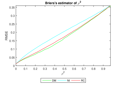
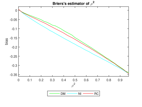
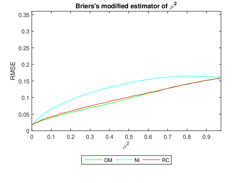
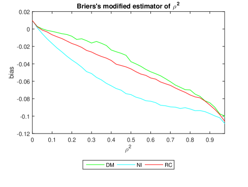
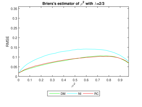
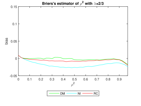
Figure 1: RMSE and bias for different estimators of $\rho^{2}$: $\widetilde{\rho}_{\widehat{n}^{\ast},N}^{2}$ (top), $\widetilde{\rho}_{\widehat{n}^{\ast},N,\bullet}^{2}$ (middle), $\widetilde{\rho}_{\widehat{n}^{\ast},N,\lambda}^{2}$ with $\lambda=2/3$ (bottom).

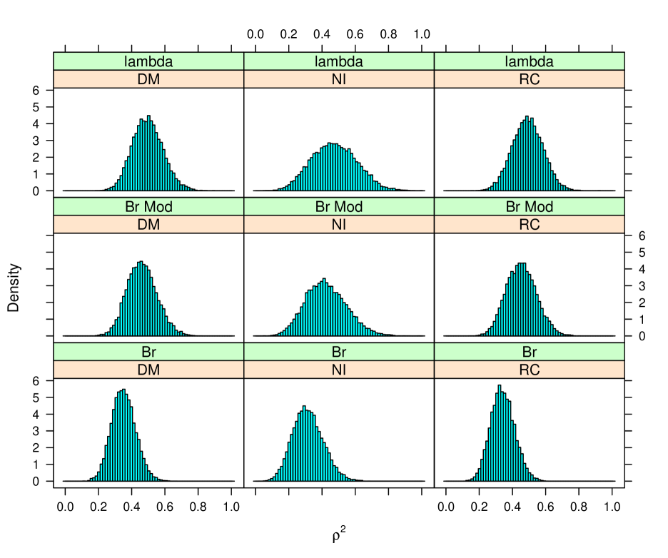
Figure 2: Density plots with estimates obtained from observations of three distributions, DM, NI, RC, when $\rho^{2}=0.5$: $\widetilde{\rho}_{\widehat{n}^{\ast},N}^{2}$ (below, Br), $\widetilde{\rho}_{\widehat{n}^{\ast},N,\bullet}^{2}$ (middle, Br Mod), $\widetilde{\rho}_{\widehat{n}^{\ast},N,\lambda}^{2}$ with $\lambda=2/3$ (top, lambda)

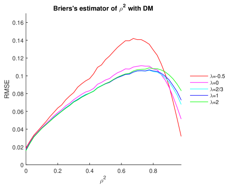
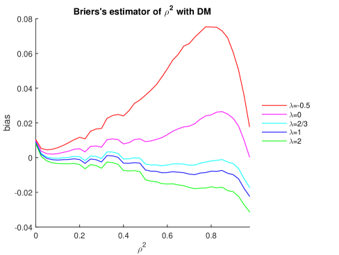
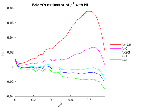
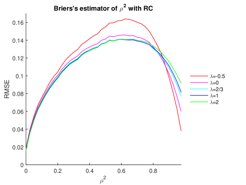
Figure 3: RMSE and bias of $\widetilde{\rho}_{\widehat{n}^{\ast},N,\lambda}^{2}$ with different values of $\lambda$ for DM (top), NI (middle), RC (bottom) distributions.

6.2 Study on FBI data (Weir and Hill, 2002)

Based on the FBI data study (Section 5.2), with theoretical values obtained from the estimates of the probability vectors given in Table 5.7 for loci D3S1358, vWA, FGA and D8S1179, the clustered multinomial distributions are studied under no underlying assumption (saturated log-linear model). Through Monte Carlo simulations, the RMSE and bias of the new estimator proposed in Section 4.3.2 ($\widehat{\rho}^{2}$) and the Weir and Hill estimator ($\overline{\rho}^{2}$) are compared in Figures 4, 5, 6, 7, focused respectively on the loci D3S1358, vWA, FGA and D8S1179. Since these kind of data have usually small values of the intracluster correlation coefficient, $\rho^{2}$, the study is only focussed on $\rho^{2}\in(0,0.1)$. Except for the RC distribution, the bias of $\widehat{\rho}^{2}$ tends to be greater than the bias of $\overline{\rho}^{2}$, however, the RMSE of $\widehat{\rho}^{2}$ tends to be smaller than the RMSE of $\overline{\rho}^{2}$. This weakness of the bias could be improved in case of being able to identify an apropriate log-linear model.

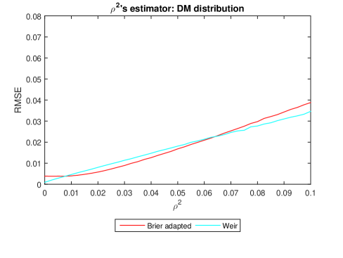
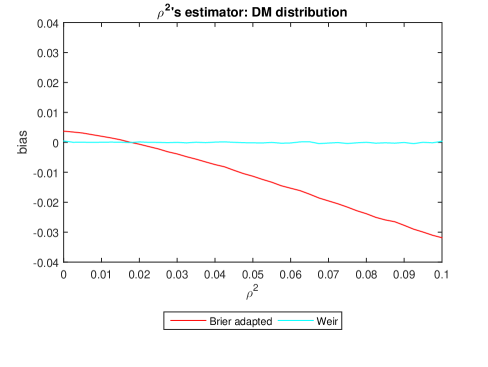
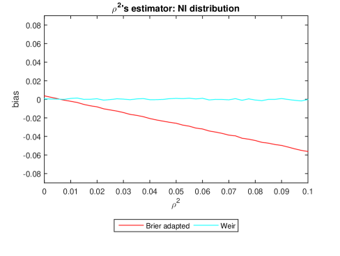
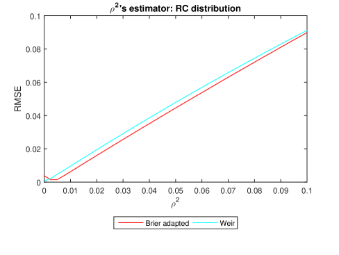
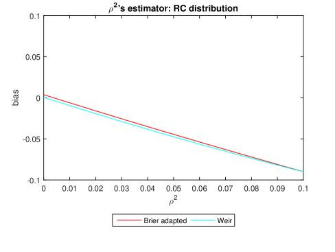
Figure 4: RMSE and bias of the Brier adapted $\widehat{\rho}^{2}$ and Weir’s $\overline{\rho}^{2}$ for small values of $\rho^{2}$ when DM, NI and RC distributions are considered and the theoretical probabilities are equal to the estimates for locus D3S1358.

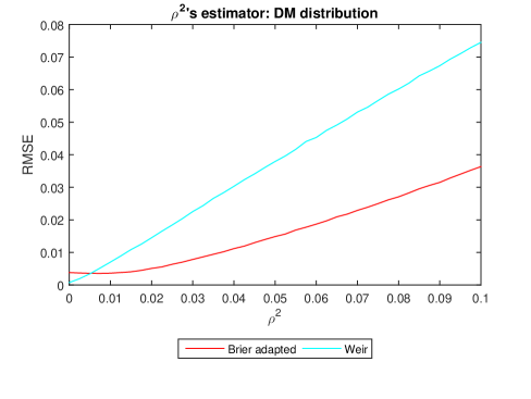
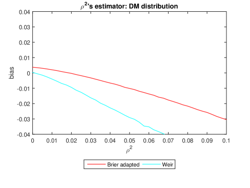
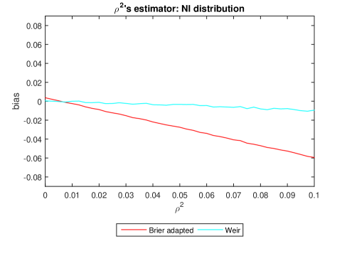
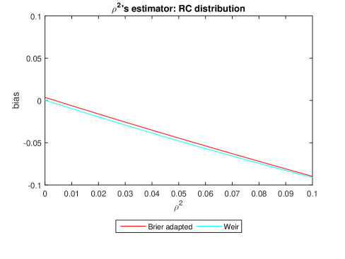
Figure 5: RMSE and bias of the Brier adapted $\widehat{\rho}^{2}$ and Weir’s $\overline{\rho}^{2}$ for small values of $\rho^{2}$ when DM, NI and RC distributions are considered and the theoretical probabilities are equal to the estimates for locus vWA.

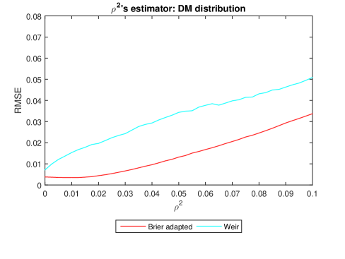
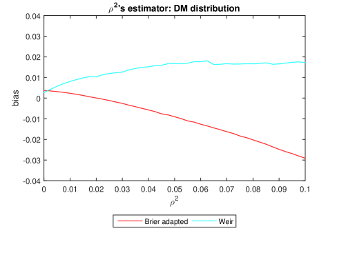
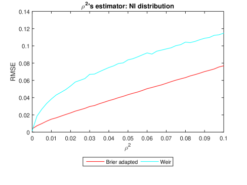
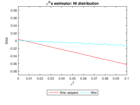
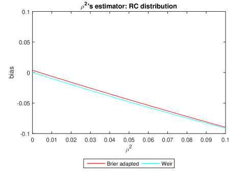
Figure 6: RMSE and bias of the Brier adapted $\widehat{\rho}^{2}$ and Weir’s $\overline{\rho}^{2}$ for small values of $\rho^{2}$ when DM, NI and RC distributions are considered and the theoretical probabilities are equal to the estimates for locus FGA.

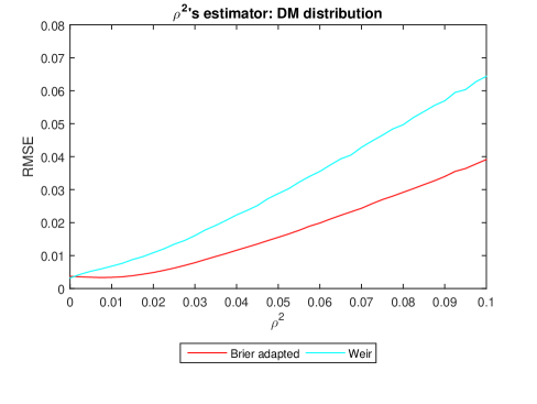
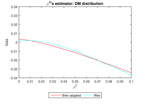
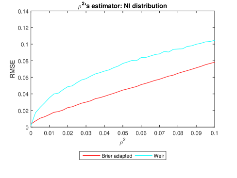
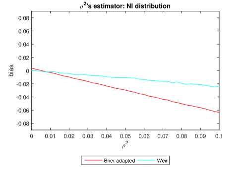
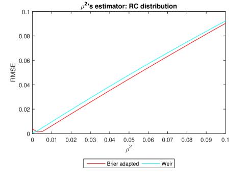
Figure 7: RMSE and bias of the Brier adapted $\widehat{\rho}^{2}$ and Weir’s $\overline{\rho}^{2}$ for small values of $\rho^{2}$ when DM, NI and RC distributions are considered and the theoretical probabilities are equal to the estimates for locus D8S1179.

7 Concluding remarks

This paper deals with log-linear models for studying the intracluster correlation coefficient in clustered multinomial data. As no distributional assumption is made, only the first two moment assumptions are considered, quasi-likelihood methods are followed. With the saturated log-linear model the non-parametric estimators of the intracluster correlation coefficient are considered, and the semi-parametric estimators arise for general log-linear models. New estimators are proposed for log-linear modeling in overdispersed clustered multinomial data with unequal cluster sizes, valid either in a non-paramateric and semi-parametric setting. Big differences are found in the Monte-Carlo simulation study, when comparing the root of the mean square error and the bias of the new estimators of the intracluster correlation coefficient with the clasical ones. In addition, quasi minimum $\phi$-divergence estimators are proposed and from the Monte Carlo experiments we saw that it is possible to decrease the root of the mean square error in comparison with the quasi-maximum likelihood estimators. These results of this paper could be extended for any generalized linear model and the new estimators are promising to improve the quality of the goodness-of-fit test statistics for log-linear models in overdispersed clustered multinomial data.

The referees suggested to us to consider the interesting problems related to mising values as well as to get the standard errors of $\widehat{\rho}_{n,N}^{2}.$ We know that the problem of missing values has been very well solved in Chapter 2 of the PhD thesis of Raim (2014) for the random clumped distribution. We think that the problem associated to missing data using the modelization given in this paper, applying log-linear models, requires a separate paper. The standard errors of $\widehat{\rho}_{n,N}^{2}$ requires also a paper in the line of the paper of Weir and Hill (2002).

Acknowledgement. We would like to thank the referees for their helpful comments and suggestions. This research is supported by the Spanish Grant MTM2012-33740 from Ministerio de Economia y Competitividad.

Appendix A Appendix

A.1 Zero-inflated binomial distribution

The binomial distribution with zero inflation in the first cell, i.e. $n$-inflation in the second cell, is given by

$$\left(\left.\begin{pmatrix}Y_{1}\\ Y_{2}\end{pmatrix}\right|V=v\right)=\left\{\begin{array}[c]{lll}\mathcal{M}\left(n,\begin{pmatrix}p_{1}(\boldsymbol{\theta})\\ p_{2}(\boldsymbol{\theta})\end{pmatrix}\right),&\text{if }v=1,&\text{with }\Pr(V=1)=w\\ n\boldsymbol{e}_{2},&\text{if }v=0,&\text{with }\Pr(V=0)=1-w\end{array}\right..$$

Its first order moment vector is given by

$$E\left[\begin{pmatrix}Y_{1}\\ Y_{2}\end{pmatrix}\right] =E\left[E\left[\left.\begin{pmatrix}Y_{1}\\ Y_{2}\end{pmatrix}\right|V\right]\right]$$

$$=E\left[\left.\begin{pmatrix}Y_{1}\\ Y_{2}\end{pmatrix}\right|V=1\right]\Pr\left(V=1\right)+E\left[\left.n\boldsymbol{e}_{2}\right|V=0\right]\Pr\left(V=0\right)$$

$$=n\begin{pmatrix}wp_{1}(\boldsymbol{\theta})\\ 1-wp_{1}(\boldsymbol{\theta})\end{pmatrix}.$$

The derivation for the the second order moment matrix calculation is given by

$$E\left[Var\left[\left.\begin{pmatrix}Y_{1}\\ Y_{2}\end{pmatrix}\right|V\right]\right] =Var\left[\left.\begin{pmatrix}Y_{1}\\ Y_{2}\end{pmatrix}\right|V=1\right]\Pr\left(V=1\right)+Var\left[\left.n\boldsymbol{e}_{2}\right|V=0\right]\Pr\left(V=0\right)$$

$$=Var\left[\mathcal{M}\left(n,\begin{pmatrix}p_{1}(\boldsymbol{\theta})\\ p_{2}(\boldsymbol{\theta})\end{pmatrix}\right)\right]w$$

$$=nwp_{1}(\boldsymbol{\theta})\left(1-p_{1}(\boldsymbol{\theta})\right)\begin{pmatrix}1&-1\\ -1&1\end{pmatrix},$$

$$Var\left[E\left[\left.\begin{pmatrix}Y_{1}\\ Y_{2}\end{pmatrix}\right|V\right]\right]$$

$$=E\left[E\left[\left.\begin{pmatrix}Y_{1}\\ Y_{2}\end{pmatrix}\right|V\right]E^{T}\left[\left.\begin{pmatrix}Y_{1}\\ Y_{2}\end{pmatrix}\right|V\right]\right]-E\left[E\left[\left.\begin{pmatrix}Y_{1}\\ Y_{2}\end{pmatrix}\right|V\right]\right]E^{T}\left[E\left[\left.\begin{pmatrix}Y_{1}\\ Y_{2}\end{pmatrix}\right|V\right]\right]$$

$$=E\left[\left.\begin{pmatrix}Y_{1}\\ Y_{2}\end{pmatrix}\right|V=1\right]E^{T}\left[\left.\begin{pmatrix}Y_{1}\\ Y_{2}\end{pmatrix}\right|V=1\right]w+E\left[\left.\begin{pmatrix}Y_{1}\\ Y_{2}\end{pmatrix}\right|V=0\right]E^{T}\left[\left.\begin{pmatrix}Y_{1}\\ Y_{2}\end{pmatrix}\right|V=0\right](1-w)$$

$$-n^{2}\begin{pmatrix}wp_{1}(\boldsymbol{\theta})\\ 1-wp_{1}(\boldsymbol{\theta})\end{pmatrix}\begin{pmatrix}wp_{1}(\boldsymbol{\theta})&1-wp_{1}(\boldsymbol{\theta})\end{pmatrix}$$

$$=n^{2}(1-w)wp_{1}^{2}(\boldsymbol{\theta})\begin{pmatrix}1&-1\\ -1&1\end{pmatrix},$$

and hence

$$Var\left[\begin{pmatrix}Y_{1}\\ Y_{2}\end{pmatrix}\right] =E\left[Var\left[\left.\begin{pmatrix}Y_{1}\\ Y_{2}\end{pmatrix}\right|V\right]\right]+Var\left[E\left[\left.\begin{pmatrix}Y_{1}\\ Y_{2}\end{pmatrix}\right|V\right]\right]$$

$$=nwp_{1}(\boldsymbol{\theta})\left[\left(1-p_{1}(\boldsymbol{\theta})\right)+n(1-w)p_{1}(\boldsymbol{\theta})\right]\begin{pmatrix}1&-1\\ -1&1\end{pmatrix}$$

$$=nwp_{1}(\boldsymbol{\theta})(1-wp_{1}(\boldsymbol{\theta}))(1+\rho^{2}(n-1))\begin{pmatrix}1&-1\\ -1&1\end{pmatrix},$$

where

$$\rho^{2}=\frac{(1-w)p_{1}(\boldsymbol{\theta})}{1-wp_{1}(\boldsymbol{\theta})},\quad\text{for any }w\in(0,1).$$

This result matches the one given in Morel and Neerchal (2012, page 83). Let

$$\left(\left.\boldsymbol{Y}\right|V=v\right)=\left\{\begin{array}[c]{lll}\mathcal{M}\left(n,\boldsymbol{p}(\boldsymbol{\theta})\right),&\text{if }v=1,&\text{with }\Pr(V=1)=w\\ n\boldsymbol{e}_{M},&\text{if }v=0,&\text{with }\Pr(V=0)=1-w\end{array}\right.$$

be the multinomial distribution with zero inflation in the first $M-1$ cells, i.e. $n$-inflation in the $M$-th cell.

For $M\geq 3$, a univariate homogeneous intraclass correlation coefficient, $\rho^{2}$, seems not to be an appropriate measure to characterize the variability of this distribution, since the intraclass correlation along the cells seems to be heterogeous. The reason for this is that for $M\geq 3$ there is not an expression for the variance-covariance matrix of the multinomial distribution defined as a matrix not depending on parameters multiplied by a scalar with all the information about the parameters of the distribution.

A.2 Proof of Theorem 3.2

Let

$$\boldsymbol{S}_{\boldsymbol{Y}}=\frac{1}{N-1}\sum_{\ell=1}^{N}\left(\boldsymbol{Y}^{(\ell)}-n\widehat{\boldsymbol{p}}\right)\left(\boldsymbol{Y}^{(\ell)}-n\widehat{\boldsymbol{p}}\right)^{T},$$

the matrix of quasi-variances and quasi-covariances of the simple random sample $\boldsymbol{Y}^{(1)},...,\boldsymbol{Y}^{(N)}$ and

$$\overline{\boldsymbol{S}}_{\boldsymbol{Y}} =\mathrm{diag}(\boldsymbol{S}_{\boldsymbol{Y}})=\begin{pmatrix}S_{Y_{1}}^{2}&&\\ &\ddots&\\ &&S_{Y_{M}}^{2}\end{pmatrix},$$

$$S_{Y_{r}}^{2} =\frac{1}{N-1}\sum_{\ell=1}^{N}(Y^{(\ell,r)}-n\widehat{p}_{r})^{2}.$$

It is well-known that each diagonal element of $\overline{\boldsymbol{S}}_{\boldsymbol{Y}}$ is a consistent estimator of each diagonal element of $\vartheta_{n}n\boldsymbol{\Sigma}_{\boldsymbol{p}(\boldsymbol{\theta})}$, i.e.

$$\mathrm{E}\left[\overline{\boldsymbol{S}}_{\boldsymbol{Y}}\right]=\mathrm{diag}\{\mathrm{E}\left[\boldsymbol{S}_{\boldsymbol{Y}}\right]\}=\mathrm{diag}\{\mathrm{Var}[\boldsymbol{Y}^{(\ell)}]\}=\mathrm{diag}\{\vartheta_{n}n\boldsymbol{\Sigma}_{\boldsymbol{p}(\boldsymbol{\theta})}\},$$

and

$$S_{Y_{r}}^{2}\overset{P}{\underset{N\rightarrow\infty}{\longrightarrow}}\vartheta_{n}np_{r}(\boldsymbol{\theta})\left(1-p_{r}(\boldsymbol{\theta})\right),\quad r=1,...,M,$$ (A.1)

$$\text{or}\quad\overline{\boldsymbol{S}}_{\boldsymbol{Y}}\overset{P}{\underset{N\rightarrow\infty}{\longrightarrow}}\mathrm{diag}(\vartheta_{n}n\boldsymbol{\Sigma}_{\boldsymbol{p}(\boldsymbol{\theta})}).$$

It is not difficult to establish that

$$\mathrm{trace}(\overline{\boldsymbol{S}}_{\boldsymbol{Y}})=\sum_{r=1}^{M}S_{Y_{r}}^{2}=\mathrm{trace}(\boldsymbol{S}_{\boldsymbol{Y}})=\frac{1}{N-1}\sum_{\ell=1}^{N}\left(\boldsymbol{Y}^{(\ell)}-n\widehat{\boldsymbol{p}}\right)^{T}\left(\boldsymbol{Y}^{(\ell)}-n\widehat{\boldsymbol{p}}\right),$$ (A.2)

which is consistent for $\mathrm{trace}(\vartheta_{n}n\boldsymbol{\Sigma}_{\boldsymbol{p}(\boldsymbol{\theta})})=\vartheta_{n}n\sum_{r=1}^{M}p_{r}(\boldsymbol{\theta})\left(1-p_{r}(\boldsymbol{\theta})\right)$. We know that the chi-square test-statistic $X^{2}(\widetilde{\boldsymbol{Y}})$, given in (3.3), has an asymptotic $\mathcal{\chi}_{(N-1)(M-1)}^{2}$ distribution for fixed values of number of clusters $N$ and an increasing cluster size, $n$, under the assumption of inter-cluster level homogeneity. However, this distribution is not a useful device for the proof. Based on the expression of the chi-square test-statistic, $X^{2}(\widetilde{\boldsymbol{Y}})$, in terms of the variance-covariance matrix, as well as the same steps to obtain the expression and consistency of (A.2), we are going to establish (3.4). We have

$$\mathrm{trace}(\overline{\boldsymbol{S}}_{\boldsymbol{Y}}\tfrac{1}{n}\boldsymbol{D}_{\boldsymbol{p}(\boldsymbol{\theta})}^{-1})=\frac{1}{N-1}\sum_{\ell=1}^{N}\left(\boldsymbol{Y}^{(\ell)}-n\widehat{\boldsymbol{p}}\right)^{T}\tfrac{1}{n}\boldsymbol{D}_{\boldsymbol{p}(\boldsymbol{\theta})}^{-1}\left(\boldsymbol{Y}^{(\ell)}-n\widehat{\boldsymbol{p}}\right)$$

and

$$\mathrm{E}\left[\mathrm{trace}(\overline{\boldsymbol{S}}_{\boldsymbol{Y}}\tfrac{1}{n}\boldsymbol{D}_{\boldsymbol{p}(\boldsymbol{\theta})}^{-1})\right] =\mathrm{traceE}\left[\overline{\boldsymbol{S}}_{\boldsymbol{Y}}\tfrac{1}{n}\boldsymbol{D}_{\boldsymbol{p}(\boldsymbol{\theta})}^{-1}\right]=\mathrm{trace}\left(\mathrm{E}\left[\overline{\boldsymbol{S}}_{\boldsymbol{Y}}\right]\tfrac{1}{n}\boldsymbol{D}_{\boldsymbol{p}(\boldsymbol{\theta})}^{-1}\right)=\mathrm{trace}\left(\vartheta_{n}n\boldsymbol{\Sigma}_{\boldsymbol{p}(\boldsymbol{\theta})}\tfrac{1}{n}\boldsymbol{D}_{\boldsymbol{p}(\boldsymbol{\theta})}^{-1}\right)$$

$$=\vartheta_{n}\mathrm{trace}\left(\boldsymbol{\Sigma}_{\boldsymbol{p}(\boldsymbol{\theta})}\boldsymbol{D}_{\boldsymbol{p}(\boldsymbol{\theta})}^{-1}\right)=\vartheta_{n}\mathrm{trace}\left(\left(\boldsymbol{D}_{\boldsymbol{p}(\boldsymbol{\theta})}-\boldsymbol{p}(\boldsymbol{\theta})\boldsymbol{p}^{T}(\boldsymbol{\theta})\right)\boldsymbol{D}_{\boldsymbol{p}(\boldsymbol{\theta})}^{-1}\right)$$

$$=\vartheta_{n}\left[\mathrm{trace}(\boldsymbol{I}_{M})-\mathrm{trace}(\boldsymbol{p}(\boldsymbol{\theta})\boldsymbol{1}_{M}^{T})\right]=\vartheta_{n}(M-1).$$

Hence,

$$\mathrm{E}\left[\frac{1}{M-1}\mathrm{trace}(\overline{\boldsymbol{S}}_{\boldsymbol{Y}}\tfrac{1}{n}\boldsymbol{D}_{\boldsymbol{p}(\boldsymbol{\theta})}^{-1})\right]=\mathrm{E}\left[\frac{1}{(N-1)(M-1)}\sum_{\ell=1}^{N}\left(\boldsymbol{Y}^{(\ell)}-n\widehat{\boldsymbol{p}}\right)^{T}\tfrac{1}{n}\boldsymbol{D}_{\boldsymbol{p}(\boldsymbol{\theta})}^{-1}\left(\boldsymbol{Y}^{(\ell)}-n\widehat{\boldsymbol{p}}\right)\right]=\vartheta_{n},$$

and taking into account that $\widehat{\boldsymbol{p}}$ is a consistent estimator of $\boldsymbol{p}(\boldsymbol{\theta})$, as $N\rightarrow\infty$, as well as (A.1),

$$\frac{1}{M-1}\mathrm{trace}(\overline{\boldsymbol{S}}_{\boldsymbol{Y}}\tfrac{1}{n}\boldsymbol{D}_{\widehat{\boldsymbol{p}}}^{-1})=\frac{1}{(N-1)(M-1)}\sum_{\ell=1}^{N}\left(\boldsymbol{Y}^{(\ell)}-n\widehat{\boldsymbol{p}}\right)^{T}\tfrac{1}{n}\boldsymbol{D}_{\widehat{\boldsymbol{p}}}^{-1}\left(\boldsymbol{Y}^{(\ell)}-n\widehat{\boldsymbol{p}}\right)=\frac{X^{2}(\widetilde{\boldsymbol{Y}})}{(N-1)(M-1)}$$

tends in probability to $\vartheta_{n}$, as $N\rightarrow\infty$. In other words,

$$\frac{X^{2}(\widetilde{\boldsymbol{Y}})}{(N-1)(M-1)}=\frac{1}{(M-1)n}\sum_{r=1}^{M}\frac{1}{\widehat{p}_{r}}S_{Y_{r}}^{2}\overset{P}{\underset{N\rightarrow\infty}{\longrightarrow}}\frac{\vartheta_{n}n}{(M-1)n}\sum_{r=1}^{M}\frac{p_{r}(\boldsymbol{\theta})}{p_{r}(\boldsymbol{\theta})}\left(1-p_{r}(\boldsymbol{\theta})\right)=\vartheta_{n}.$$

In addition, taking into account (1.9), the right hand size of (3.4) follows. Finally, we like to mention that even though $X^{2}(\widetilde{\boldsymbol{Y}})$ and $\vartheta_{n}(N-1)(M-1)$ have the same expectation for a fixed value of $N$, this proof is not trivial since $\vartheta_{n}(N-1)(M-1)$ as well as $X^{2}(\widetilde{\boldsymbol{Y}})$ tend to infinite as $N\rightarrow\infty$.

A.3 Proof of Theorem 2.2

By applying the Central Limit Theorem it holds (3.1). Hence, from Pardo (2006, formula (7.10)), for the minimum phi-divergence estimator of $\boldsymbol{\theta}$ of a log-linear model it holds

$$\sqrt{N}(\widehat{\boldsymbol{\theta}}_{\phi}-\boldsymbol{\theta}_{0})=\left(\boldsymbol{\boldsymbol{W}}^{T}\boldsymbol{\Sigma\boldsymbol{{}_{\boldsymbol{p}\left(\theta_{0}\right)}}W}\right)^{-1}\boldsymbol{W}^{T}\boldsymbol{\Sigma}_{p\left(\boldsymbol{\theta}_{0}\right)}\boldsymbol{D}_{\boldsymbol{p}\left(\theta_{0}\right)}^{-1}\sqrt{N}\left(\widehat{\boldsymbol{p}}-\boldsymbol{p}\left(\boldsymbol{\theta}_{0}\right)\right)+o_{p}\left(\boldsymbol{1}_{M_{0}}\right),$$ (A.3)

and the variance-covariance matrix of $\sqrt{N}(\widehat{\boldsymbol{\theta}}_{\phi}-\boldsymbol{\theta}_{0})$ is

$$\tfrac{\vartheta_{n}}{n}\left(\boldsymbol{\boldsymbol{W}}^{T}\boldsymbol{\Sigma\boldsymbol{{}_{\boldsymbol{p}\left(\theta_{0}\right)}}W}\right)^{-1}\boldsymbol{W}^{T}\boldsymbol{\Sigma}_{p\left(\boldsymbol{\theta}_{0}\right)}\boldsymbol{D}_{\boldsymbol{p}\left(\theta_{0}\right)}^{-1}\boldsymbol{\Sigma}_{\boldsymbol{p}\left(\boldsymbol{\theta}_{0}\right)}\boldsymbol{D}_{\boldsymbol{p}\left(\theta_{0}\right)}^{-1}\boldsymbol{\Sigma}_{\boldsymbol{p}\left(\boldsymbol{\theta}_{0}\right)}\boldsymbol{W}\left(\boldsymbol{\boldsymbol{W}}^{T}\boldsymbol{\Sigma\boldsymbol{{}_{\boldsymbol{p}\left(\theta_{0}\right)}}W}\right)^{-1}$$

$$=\tfrac{\vartheta_{n}}{n}\left(\boldsymbol{\boldsymbol{W}}^{T}\boldsymbol{\Sigma\boldsymbol{{}_{\boldsymbol{p}\left(\theta_{0}\right)}}W}\right)^{-1}.$$ (A.4)

The last equality comes from

$$\boldsymbol{\Sigma}_{\boldsymbol{p}\left(\boldsymbol{\theta}_{0}\right)}\boldsymbol{D}_{\boldsymbol{p}\left(\theta_{0}\right)}^{-1}\boldsymbol{\Sigma}_{\boldsymbol{p}\left(\boldsymbol{\theta}_{0}\right)}=\boldsymbol{\Sigma}_{\boldsymbol{p}\left(\boldsymbol{\theta}_{0}\right)}.$$

From the Taylor expansion of $\boldsymbol{p}(\widehat{\boldsymbol{\theta}}_{\phi})$ around $\boldsymbol{p}(\boldsymbol{\theta}_{0})$ we obtain

$$\sqrt{N}(\boldsymbol{p}(\widehat{\boldsymbol{\theta}}_{\phi})-\boldsymbol{p}(\boldsymbol{\theta}_{0}))=\boldsymbol{\Sigma\boldsymbol{{}_{\boldsymbol{p}\left(\theta_{0}\right)}}W}\sqrt{N}(\widehat{\boldsymbol{\theta}}_{\phi}-\boldsymbol{\theta}_{0})+o_{p}\left(\boldsymbol{1}_{M}\right),$$ (A.5)

and the variance-covariance matrix of $\sqrt{N}(\boldsymbol{p}(\widehat{\boldsymbol{\theta}}_{\phi})-\boldsymbol{p}(\boldsymbol{\theta}_{0}))$ is

$$\tfrac{\vartheta_{n}}{n}\boldsymbol{\Sigma\boldsymbol{{}_{\boldsymbol{p}\left(\theta_{0}\right)}}W}\left(\boldsymbol{\boldsymbol{W}}^{T}\boldsymbol{\Sigma\boldsymbol{{}_{\boldsymbol{p}\left(\theta_{0}\right)}}W}\right)^{-1}\boldsymbol{W}^{T}\boldsymbol{\Sigma}_{p\left(\boldsymbol{\theta}_{0}\right)}.$$ (A.6)

Since $\sqrt{N}\left(\widehat{\boldsymbol{p}}-\boldsymbol{p}\left(\boldsymbol{\theta}_{0}\right)\right)$ is normal and centred, from (A.3) and (A.4), (2.8) is obtained. Similarly, since $\sqrt{N}(\widehat{\boldsymbol{\theta}}_{\phi}-\boldsymbol{\theta}_{0})$ is normal and centred, from (A.5) and (A.6), (2.9) is obtained.

A.4 Derivation of Formula (4.4)

Multiplying (4.3) by $\left.\sqrt{N_{g}}n_{g}\right/\sum\limits_{h=1}^{G}n_{h}N_{h}$

$$w_{g}(\widehat{\boldsymbol{p}}^{(g)}-\boldsymbol{p}\left(\boldsymbol{\theta}_{0}\right))\overset{\mathcal{L}}{\underset{N_{g}\rightarrow\infty}{\longrightarrow}}\mathcal{N}\left(\boldsymbol{0}_{M},\tfrac{n_{g}N_{g}\vartheta_{n_{g}}}{\left(\sum\nolimits_{h=1}^{G}n_{h}N_{h}\right)^{2}}\boldsymbol{\Sigma}_{\boldsymbol{p}\left(\boldsymbol{\theta}_{0}\right)}\right),$$

hence summing up from $g=1$ to $G$ and by the independence of clusters

$$\sum\limits_{g=1}^{G}w_{g}(\widehat{\boldsymbol{p}}^{\left(g\right)}-\boldsymbol{p}\left(\boldsymbol{\theta}_{0}\right))=\left(\widehat{\boldsymbol{p}}-\boldsymbol{p}\left(\boldsymbol{\theta}_{0}\right)\right)\overset{\mathcal{L}}{\underset{N_{g}\rightarrow\infty,\;g=1,...,G}{\longrightarrow}}\mathcal{N}\left(\boldsymbol{0}_{M},\tfrac{\sum\nolimits_{g=1}^{G}n_{g}N_{g}\vartheta_{n_{g}}}{\left(\sum\nolimits_{h=1}^{G}n_{h}N_{h}\right)^{2}}\boldsymbol{\Sigma}_{\boldsymbol{p}\left(\boldsymbol{\theta}_{0}\right)}\right).$$

Finally multiplying the previous expression by $\left.\sum\nolimits_{h=1}^{G}n_{h}N_{h}\right/\sqrt{\sum\nolimits_{g=1}^{G}n_{g}N_{g}\vartheta_{n_{g}}}$, the desired expression is obtained.

A.5 Algorithms for Dirichlet-multinomial, n-inflated and random-clumped distributions

The usual parameters of the $M$-dimensional random variable $\boldsymbol{Y}=(Y_{1},...,Y_{M})^{T}$ with Dirichlet-multinomial distribution are $\boldsymbol{\alpha}=\left(\alpha_{11},...,\alpha_{M1}\right)^{T}$, where $\alpha_{r1}=\frac{1-\rho^{2}}{\rho^{2}}p_{r}\left(\boldsymbol{\theta}\right)$, $r=1,...,M$. For convenience it is considered with parameters $\boldsymbol{\beta}=\begin{pmatrix}\rho^{2}\\ \boldsymbol{p}(\boldsymbol{\theta})\end{pmatrix}$, $\boldsymbol{p}\left(\boldsymbol{\theta}\right)=\left(p_{1}\left(\boldsymbol{\theta}\right),...,p_{M}\left(\boldsymbol{\theta}\right)\right)^{T}$, and is generated as follows:
STEP 1. Generate $B_{1}\sim Beta(\alpha_{11},\alpha_{12})$, with $\alpha_{11}=\frac{1-\rho^{2}}{\rho^{2}}p_{1}\left(\boldsymbol{\theta}\right)$, $\alpha_{12}=\frac{1-\rho^{2}}{\rho^{2}}(1-p_{1}\left(\boldsymbol{\theta}\right))$.
STEP 2. Generate $\left(Y_{1}|B_{1}=b_{1}\right)\sim Bin(n,b_{1})$.
STEP 3. For $r=2,...,M-1$ do:
             Generate $B_{r}\sim Beta(\alpha_{r1},\alpha_{r2})$, with $\alpha_{r1}=\frac{1-\rho^{2}}{\rho^{2}}p_{r}\left(\boldsymbol{\theta}\right)$, $\alpha_{r2}=\frac{1-\rho^{2}}{\rho^{2}}\left(1-\sum\limits_{h=1}^{r}p_{h}\left(\boldsymbol{\theta}\right)\right)$.
             Generate $\left(Y_{r}|Y_{1}=y_{1},...,Y_{r-1}=y_{r-1},B_{r}=b_{r}\right)\sim Bin\left(n-\sum\limits_{h=1}^{r-1}y_{h},b_{r}\right)$.
STEP 4. Do $\left(Y_{M}|Y_{1}=y_{1},...,Y_{M-1}=y_{M-1}\right)=n-\sum\limits_{h=1}^{M-1}y_{h}$.

The random variable $\boldsymbol{Y}=(Y_{1},...,Y_{M})^{T}$ of the $n$-inflated multinomial distribution with parameters $\boldsymbol{\beta}$, $\boldsymbol{p}\left(\boldsymbol{\theta}\right)$, is generated as follows:
STEP 1. Generate $V\sim Ber(\rho^{2})$.
STEP 2. Generate

$$\mathtt{\ }\left(\boldsymbol{Y|}V=v\right)=\left\{\begin{array}[c]{ll}\mathcal{M}(n,\boldsymbol{p}\left(\boldsymbol{\theta}\right)),&\text{if }v=0\\ n\mathcal{M}(1,\boldsymbol{p}\left(\boldsymbol{\theta}\right)),&\text{if }v=1\end{array}\right..$$

The random variable $\boldsymbol{Y}=(Y_{1},...,Y_{M})^{T}$ of the random clumped distribution with parameters $\boldsymbol{\beta}$, $\boldsymbol{p}\left(\boldsymbol{\theta}\right)$, is generated as follows:
STEP 1. Generate $\boldsymbol{Y}_{0}=(Y_{01},...,Y_{0M})^{T}\sim\mathcal{M}(1,\boldsymbol{p}\left(\boldsymbol{\theta}\right))$.
STEP 2. Generate $K_{1}\sim Bin(n,\rho)$.
STEP 3. Generate $\left(\boldsymbol{Y}_{1}|K_{1}=k_{1}\right)=\left((Y_{11},...,Y_{1M})^{T}|K_{1}=k_{1}\right)\sim\mathcal{M}(n-k_{1},\boldsymbol{p}\left(\boldsymbol{\theta}\right))$.
STEP 4. Do $\left(\boldsymbol{Y|}K_{1}=k_{1}\right)\boldsymbol{=Y}_{0}k_{1}+\left(\boldsymbol{Y}_{1}|K_{1}=k_{1}\right)$.
For the details about the equivalence of this algorithm and (1.12), see Morel and Nagaraj (1993).

It is interesting to note that there exists the package ”Modeling overdispersion in $R$” useful to generate the distributions considered in this Appendix. For more details see Raim et al (2015).

References

- [1] Ahn, H. and James, J. C. (1995). Generation of Over-Dispersed and Under-Dispersed Binomial Variates. Journal of Computational and Graphical Statistics, 4, 55–64.
- [2] Altham, P. M. E. (1976). Discrete variable analysis for individuals grouped into families. Biometrika, 63, 263–269.
- [3] Bokossa, M. (1999). Parameter estimation in overdispersion models. Unpublished Ph.D. thesis, University of Maryland.
- [4] Budowle, B. and Moretti, T. R. (1999). Genotype profiles for six population groups at the 13 CODIS short tandem repeat core loci and other PCR-based loci. Forensic Science Communications 1999. Available at http://www.fbi.gov/about-us/lab/forensic-science-communications/fsc/july1999/$$budowle.htm.
- [5] Brier, S. S. (1980). Analysis of contingency tables under cluster sampling. Biometrika, 67, 591–596.
- [6] Cohen, J. E. (1976). The distribution of the chi-squared statistic under clustered sampling from contingency tables. J. Am. Statist. Assoc., 71, 665–670.
- [7] Cressie, N. and Pardo, L. (2000). Minimum -divergence estimator and hierarchical testing in loglinear models. Statistica Sinica, 10, 867–884.
- [8] Cressie, N., Pardo, L. (2002). Model checking in loglinear models using -divergences and MLEs. Journal of Statistical Planning and Inference, 103, 437–453.
- [9] Cressie, N., Pardo, L. and Pardo, M.C. (2003). Size and power considerations for testing loglinear models using -divergence test statistics. Statistica Sinica, 13, 555–570.
- [10] Hall, D. B. (2000). Zero-Inflated Poisson and Binomial Regression with Random Effects: A Case Study, Biometrics 56, 1030–1039.
- [11] Martín, N. and Pardo, L. (2008a). New families of estimators and test statistics in log-linear models. Journal of Multivariate Analysis, 99, 1590–1609.
- [12] Martín, N. and Pardo, L. (2008b). Minimum phi-divergence estimators for loglinear models with linear constraints and multinomial sampling, Statistical Papers, 49, 15–36
- [13] Martín, N. and Pardo, L. (2010). A new measure of leverage cells in multinomial loglinear models. Communications in Statistics - Theory and Methods, 39, 517–530.
- [14] Martín, N. and Pardo, L. (2011). Fitting DNA sequences through log-linear modelling with linear constraints. Statistics, 45, 605–621.
- [15] Martín, N. and Pardo, L. (2012). Poisson loglinear modeling with linear constraints on the expected cell frequencies. Sankhya: The Indian Journal of Statistics, 74B, 238–267.
- [16] Menéndez, M. L., Morales, D., Pardo, L. and Vajda, I. (1995). Divergence-based estimation and testing of statistical models of classification. Journal of Multivariate Analysis, 54, 329–354
- [17] Menéndez, M. L., Morales, D., Pardo, L. and Vajda, I. (1996). About divergence-based goodness-of-fit tests in the Dirichlet-multinomial model. Communications in Statistics - Theory and Methods, 25, 1119–1133.
- [18] Morel, J.G. and Nagaraj, N.K. (1993). A finite mixture distribution for modelling multinomial extra variation. Biometrika, 80, 363–371.
- [19] Neerchal, N.K. and Morel, J.G. (1998). Large cluster results for two parametric multinomial extra variation models. Journal of the American Statistical Association, 93, 1078–1087.
- [20] Mosimann, J. E. (1962). On the compound multinomial distributions, the multivariate -distribution and correlation among proportions. Biometrika, 49, 65–82.
- [21] Pardo, L. (2006). Statistical inference based on divergence measures. Chapman & Hall/CRC, Boca Raton.
- [22] Raim, A. M. (2014). Computational Methods for Finite Mixtures using Approximate Information and Regression Linked to the Mixture Mean. PhD Thesis, University of Mayland.
- [23] Raim, A. M. , Neerchal, N. K. and Morel, J. G. (2015). Modeling overdispersion in Technical Report HPCI-2015-1 UMBCH High Performance Computing Facility, University of Maryland, Baltimore Country, 2015.
- [24] Vos, P. W. (1992). Minimum f-divergence estimators and quasi-likelihood functions. Annals of the Institute of Statistical Mathematics, 44, 261–279.
- [25] Wedderburn, R. W. M. (1974). Quasi-likelihood functions, generalized linear models, and the Gauss-Newton method. Biometrika, 61, 439–447.
- [26] Weir, B. S. and Hill, W. G. (2002). Estimating F-statistics. Annual Review of Genetics, 36, 721–750.