Topological Characterization of Extended Quantum Ising Models

Abstract

We show that a class of exactly solvable quantum Ising models, including the transverse-field Ising model and anisotropic $XY$ model, can be characterized as the loops in a two-dimensional auxiliary space. The transverse-field Ising model corresponds to a circle and the $XY$ model corresponds to an ellipse, while other models yield cardioid, limacon, hypocycloid, and Lissajous curves etc. It is shown that the variation of the ground state energy density, which is a function of the loop, experiences a nonanalytical point when the winding number of the corresponding loop changes. The winding number can serve as a topological quantum number of the quantum phases in the extended quantum Ising model, which sheds some light upon the relation between quantum phase transition and the geometrical order parameter characterizing the phase diagram.

Introduction. Characterizing the quantum phase transitions (QPTs) is of central significance to both condensed matter physics and quantum information science. QPTs occur only at zero temperature due to the competition between different parameters describing the interactions of the system. A quantitative understanding of the second-order QPT is that the ground state undergoes qualitative changes when an external parameter passes through quantum critical points (QCPs).

There are two prototypical models, Bose-Hubbard model and transverse-field Ising model, based on which the concept and characteristic of QPTs can be well demonstrated. However, among the two, only the transverse-field Ising model is exactly solvable SachdevBook , so as to be a unique paradigm for understanding the QPTs. Recently, more attention has been paid to theoretical studies of exactly solvable quantum spin models involving nearest-, next-nearest-neighbor interactions, and multiple spin exchange models, etc Titvinidze03 ; Tsvelik90 ; Frahm92 ; Muramoto99 ; Zvyagin01 ; Zvyagin03 ; Lou04 ; Zvyagin05 . Those models are closer to real quasi-one-dimensional magnets Zheludev00 ; Tsukada00 ; Kohgi01 comparing to standard ones with only nearest-neighbor couplings. Furthermore, it has been shown that quantum spin models can be simulated in artificial quantum system with controllable parameters. Quantum simulation of spin chain can be experimentally realized through neutral atoms stored in an optical lattice Simon11 ; Struck11 , trapped ions Porras04 ; Deng05 ; Taylor08 ; Friedenauer08 ; Kim10 ; Edwards10 ; Kim11 ; Kim09 ; Islam11 and NMR simulator Li14 . This system often serves as a test bed for applying new ideas and methods to quantum phase transitions.

A fundamental question is whether QPTs in Ising model can have a connection to some topological characterizations. It is interesting to note in this context that some simple Ising models have been found to exhibit topological characterization Lee07 ; Feng07 ; DeGottardi11 ; Zhang11 . The purpose of the present work is to shed some light upon the relation between QPTs and a geometrical parameter characterizing the phase diagram, through the investigation of a class of quantum Ising models.

In this work, we present an extended quantum Ising model, which includes an additional three-body interaction. It can be exactly solved by the routine procedure, taking the Jordan-Wigner and pseudo-spin transformations. Based on the exact solution, we investigate the QPT in this model. We introduce a global order parameter, which is the winding number for the loop specifying to a set of coupling constants, in an auxiliary space. The ground state energy density can be a function of the loop and its variation experiences a nonanalytical point when the winding number of the corresponding loop changes. Then the relation between QPTs and the geometrical order parameter is established.

Extended Ising model and solutions. We start our analysis from the one-dimensional Ising model, which has the Hamiltonian

$$H = \sum\limits_{j=1}^{N}[a\left(\frac{1+\gamma}{2}\sigma_{j}^{x}\sigma_{j+1}^{x}+\frac{1-\gamma}{2}\sigma_{j}^{y}\sigma_{j+1}^{y}\right)+g\sigma_{j}^{z}$$ (1)

$$+b\sigma_{j}^{z}\left(\frac{1+\delta}{2}\sigma_{j-1}^{x}\sigma_{j+1}^{x}+\frac{1-\delta}{2}\sigma_{j-1}^{y}\sigma_{j+1}^{y}\right)],$$

where $\sigma_{j}^{\alpha}$, for $\alpha=x,y,z,$ are the usual Pauli matrices, and periodic boundary conditions are assumed. Comparing with the customary anisotropic $XY$ model, there are additional three-site interactions $\sigma_{j}^{z}\sigma_{j-1}^{x}\sigma_{j+1}^{x}$ and $\sigma_{j}^{z}\sigma_{j-1}^{y}\sigma_{j+1}^{y}$, which have the following two implications: it can be either regarded as the conditional anisotropic $XY$-type coupling between next-nearest-neighbor spins, or conditional action of transverse field. The ground state phase diagram and correlation functions for this spin model have been studied 40 years ago Suzuki71 . In the case of $g=\gamma=\delta=0$, the correlation function has been obtained Titvinidze03 . In addition, other types of Hamiltonians which contain three-body interactions were also investigated Zvyagin06 ; Divakaran13 ; Zhang12 .

We will see that this model can be exactly solvable in a simple way by the similar procedure for the simple transverse-field Ising model SachdevBook ; Dziarmaga ; Pfeuty . For the sake of simplicity, we only concern the case of even $N$, the conclusion is available for the case of odd $N$ in the thermodynamic limit. As the same procedure performed in solving the Hamiltonian without the additional term, we take the Jordan-Wigner transformation SachdevBook

$$\sigma_{j}^{z} = 1-2c_{j}^{\dagger}c_{j}\text{, }\sigma_{j}^{y}=\mathrm{i}\sigma_{j}^{x}\sigma_{j}^{z},$$ (2)

$$\sigma_{j}^{x} = -\prod\limits_{l<j}\left(1-2c_{l}^{\dagger}c_{l}\right)\left(c_{j}+c_{j}^{{\dagger}}\right),$$ (3)

to replace the Pauli operators by the fermionic operators $c_{j}$. We note that the parity of the number of fermions is a conservative quantity and then the Hamiltonian (1) can be written in the form

$$H=\left(\begin{array}[]{cc}H^{+}&0\\ 0&H^{-}\end{array}\right),$$ (4)

where

$$H^{+} = H^{-}-2\left[b\left(c_{N}^{\dagger}c_{2}+c_{1}^{\dagger}c_{N-1}+\delta c_{2}c_{N}+\delta c_{1}c_{N-1}\right)\right.$$ (5)

$$\left.+a\left(c_{N}^{{\dagger}}c_{1}+\gamma c_{1}c_{N}\right)+\mathrm{H.c.}\right]$$

and

$$H^{-} = \sum\limits_{j=1}^{N}\left[\left(g/2-gc_{j}^{\dagger}c_{j}\right)+a\left(c_{j}^{{\dagger}}c_{j+1}+\gamma c_{j+1}c_{j}\right)\right.$$ (6)

$$\left.+b\left(c_{j}^{\dagger}c_{j+2}+\delta c_{j+2}c_{j}\right)\right]+\mathrm{H.c.}$$

are corresponding reduced Hamiltonians in the invariant subspaces with even and odd number of fermions. Here $H^{+}$ represents a fermionic ring threaded by a half of the flux quantum. In the following, we will focus on $H^{+}$ since the ground state has even parity for any values of parameters. Similarly, $H^{+}$ can be diagonalized by Fourier and pseudo-spin transformations. Taking the Fourier transformation

$$c_{j}=\frac{1}{\sqrt{N}}\sum_{k}c_{k}e^{ikj},$$ (7)

where $k=2\pi\left(m+1/2\right)/N,m=0,1,2,\ldots,N-1,$ the Hamiltonian $H^{+}$ can be expressed as a compact form

$$H^{+} = 4\sum\limits_{k>0}\overrightarrow{r}\left(k\right)\cdot\overrightarrow{s}_{k},$$ (8)

$$\overrightarrow{r}\left(k\right) = \left(0,a\gamma\sin k+b\delta\sin 2k,a\cos k+b\cos 2k-g\right),\text{\ \ \ \ \ }$$ (9)

which represents a set of pseudo spins $\left\{\overrightarrow{s}_{k}\right\}$ in a two-dimensional magnetic field $\overrightarrow{r}$. The pseudo spin is defined as

$$s_{k}^{-} = \left(s_{k}^{+}\right)^{{\dagger}}=c_{k}c_{-k},$$ (10)

$$s_{k}^{z} = \frac{1}{2}\left(c_{k}^{{\dagger}}c_{k}+c_{-k}^{{\dagger}}c_{-k}-1\right),$$ (11)

satisfying the SU(2) algebra $\left[s_{k}^{z},s_{k^{\prime}}^{\pm}\right]=\pm\delta_{kk^{\prime}}s_{k^{\prime}}^{\pm}$, $\left[s_{k}^{+},s_{k^{\prime}}^{-}\right]=2\delta_{kk^{\prime}}s_{k^{\prime}}^{z}.$ It is clear that the equivalent Hamiltonian (8) represents a system of spin ensemble in a monopole field. These spins locate at the points on the loop of $\overrightarrow{r}\left(k\right)$ defined in Eq. (9). In the following argument, we do not restrict the shape of the loop. The obtained result is valid for an arbitrary loop, which is schematically illustrated in 1(a). The Hamiltonian (8) is easy to be diagonalized by aligning all spins with the local magnetic field, which is the essential of the Bogoliubov transformation. In the thermodynamic limit, the ground state energy density can be expressed by an integration

$$\varepsilon_{g}=\lim_{N\rightarrow\infty}\frac{E_{g}}{N}=-\frac{1}{2\pi}\int\limits_{-\pi}^{\pi}\left|\overrightarrow{r}\left(k\right)\right|\mathrm{d}k,$$ (12)

which corresponds to a loop tracing with the parametric equation $\overrightarrow{r}\left(k\right)=\left(0,x\left(k\right),y\left(k\right)\right)$. In our case, the parametric equation has the form

$$\left\{\begin{array}[]{c}x\left(k\right)=a\gamma\sin k+b\delta\sin\left(2k\right)\\ y\left(k\right)=a\cos k+b\cos\left(2k\right)-g\end{array}\right.$$ (13)

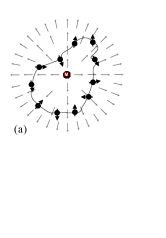
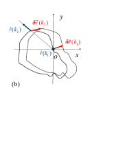
Figure 1: (Color online) Schematically illustration of the equivalent Hamiltonian (8), which represents a system of spin ensemble in a monopole field. In the thermodynamic limit, the ground state energy density becomes an integration corresponding to a loop. (b) Schematics of two loops $l$ and $l^{\prime}$ described by the parametric equations involving vectors $\overrightarrow{r}\left(k\right)$ and $\overrightarrow{r}\left(k\right)+\delta\overrightarrow{r}\left(k\right)$, respectively. Here $\overrightarrow{r}\left(k_{1}\right)$ represents an arbitrary point on the $l$, while $\overrightarrow{r}\left(k_{1}\right)+\delta\overrightarrow{r}\left(k_{1}\right)$ represents the corresponding point on the $l^{\prime}$. The red arrow indicates $\delta\overrightarrow{r}\left(k_{1}\right)$, while the blue arrow indicates the corresponding unitary vector $\hat{r}\left(k_{1}\right)$. The inner product between them $\delta\overrightarrow{r}\left(k_{1}\right)\cdot\hat{r}\left(k_{1}\right)$ contributes to the variation of $\varepsilon_{g}$. The loop $l$ passes the origin at point $\overrightarrow{r}\left(k\right)$ with $k=k_{0}$. The corresponding unitary vector $\hat{r}\left(k_{0}\right)$ is indefinite, which is denoted as a solid blue circle. The indefiniteness of $\delta\overrightarrow{r}\left(k_{0}\right)\cdot\hat{r}\left(k_{0}\right)$ witnesses the QPT as well as the topological change of the loop: enclosing the origin or not.

in the auxiliary space $\left(x,y\right)$. Then we can use some simple loops to represent the ground state of the Ising-like model. It offers many types of graphs corresponding different kinds of Ising model. To demonstrate this point, we plot several types of graphs in Fig. 2. It shows that two familiar models, transverse Ising model and anisotropic $XY$ model, correspond to two simple graphs, circle and ellipse, respectively. Rest models connect to more complicated graphs. Furthermore, the ground state of each model is naturally connected to a graph individually.

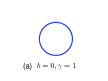
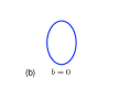
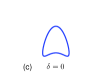
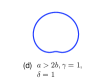
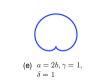
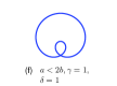
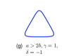
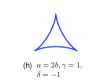
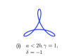
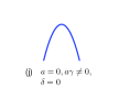
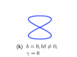
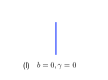
Figure 2: (Color online) several types of graphs

Quantum phase transition. In this section, we investigate the QPT occurring in the extended Ising model and its connection to the geometry of the corresponding loops. To this end, we start with the change of the ground state energy induced by varying the parameters. In general the QPT driven by the parameters $\left\{\alpha\right\}$ $\left(\alpha=a,b,\gamma,\lambda,g\right)$ can be characterized by the derivative of the ground state density with respect to $\alpha$, $\partial\varepsilon_{g}/\partial\alpha$ which experiences a nonanalytic point at the critical point, leading to the divergence of second derivative of ground state energy density. We investigate the signature of the QPT in an alternative way: $\varepsilon_{g}$ depends on the path of the integral, being a function of the functions $x\left(k\right)$ and $y\left(k\right)$. The parameters $\left\{\alpha\right\}$ drive the QPT through the change of the functions $x\left(k\right)$ and $y\left(k\right)$, or the loop. In other words, one can consider the variations of functions $x\left(k\right)$ and $y\left(k\right)$ instead of the change of the parameters $\left\{\alpha\right\}$. The first variation of the function $\varepsilon_{g}[x,y]$ is

$$\delta\varepsilon_{g}=\int\left(\frac{\delta\varepsilon_{g}}{\delta x}\delta x+\frac{\delta\varepsilon_{g}}{\delta y}\delta y\right)\mathrm{d}k=-\frac{1}{2\pi}\int\limits_{-\pi}^{\pi}\hat{r}\left(k\right)\cdot\delta\overrightarrow{r}\left(k\right)\mathrm{d}k,$$ (14)

where $\hat{r}\left(k\right)=\overrightarrow{r}/\left|\overrightarrow{r}\right|$ is the unitary vector of $\overrightarrow{r}\left(k\right)$. It indicates that the variation $\delta\varepsilon_{g}$ is the summation of the path shifts $\delta\overrightarrow{r}\left(k\right)$ along the direction of $\hat{r}\left(k\right)$. We are interested in the case of the loop crossing the origin. At the origin, the unitary vector $\hat{r}\left(k\right)$ is indefinite, which leads to an indefinite contribution to the variation $\delta\varepsilon_{g}$, indicating a nonsmooth point. It is a signature of the QPT associated with a topological change in the loop of the integration. So far, we do not specify the shape of the loop and how the loop is deformed. In our case, the variation $\delta\overrightarrow{r}\left(k\right)$ arises from the continuous change of the parameters $\left\{\alpha\right\}$. Then we have

$$\delta\overrightarrow{r}\left(k\right)=\sum_{\alpha}\frac{\partial\overrightarrow{r}\left(k\right)}{\partial\alpha}\mathrm{d}\alpha$$ (15)

or explicitly

$$\left\{\begin{array}[]{c}\delta x\left(k\right)=\sin k\left(\gamma\mathrm{d}a+a\mathrm{d}\gamma\right)+\sin\left(2k\right)\left(b\mathrm{d}\lambda+\lambda\mathrm{d}b\right)\\ \delta y\left(k\right)=\cos k\mathrm{d}a+\cos\left(2k\right)\mathrm{d}b-\mathrm{d}g\end{array}\right..$$ (16)

Considering the case with $a=\gamma=1$, $b=\lambda=0$ as an example, the Hamiltonian (1) reduces to the simplest transverse field Ising model

$$H_{\text{{Ising}}}=\sum\limits_{j=1}^{N}\left(\sigma_{j}^{x}\sigma_{j+1}^{x}+g\sigma_{j}^{z}\right),$$ (17)

the ground state energy density of which corresponds to a circle of the equation

$$x^{2}+\left(y+g\right)^{2}=1.$$ (18)

The variation $\delta\varepsilon_{g}$ from the case with $g=\pm 1$ is readily expressed as

$$\delta\varepsilon_{g}=-\frac{\mathrm{d}g}{2\pi}\int\limits_{-\pi}^{\pi}\left[\hat{r}\left(k\right)\cdot\hat{\jmath}\right]\mathrm{d}k,$$ (19)

where $\hat{\jmath}$ denotes the unit vector of $y$ axis. It results in $\delta\varepsilon_{g}=\partial\varepsilon_{g}/\partial g\mathrm{d}g$, which shows that $\delta\varepsilon_{g}$ accords with $\partial\varepsilon_{g}/\partial g$ as a witness of QPT.

We would like to point out that each loop contains two characters, geometry (shape and position) and curve orientation, which are determined by the corresponding parameter equation. To characterize these two features, we use a topological quantity, winding number, which is a fundamental concept in geometric topology and widely used in various areas of physics Park2000 ; Hatsugai93 ; Leutwyler92 ; Ezawa13 . The winding number of a closed curve in the auxiliary $xy$-plane around the origin is defined as

$$\mathcal{N}=\frac{1}{2\pi}\int\nolimits_{c}\frac{1}{r^{2}}\left(y\mathrm{d}x-x\mathrm{d}y\right),$$ (20)

which is an integer representing the total number of times that the curve travels clockwise around the origin. Then we establish the connection between the QPT and the switch of the topological quantity.

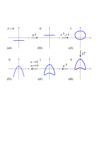
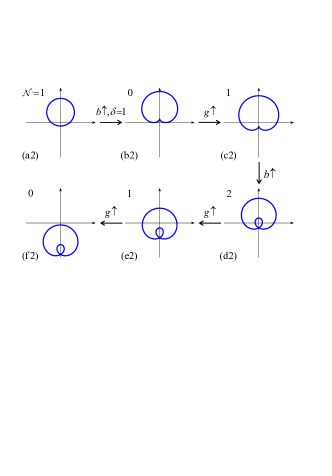
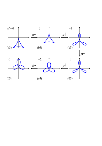
Figure 3: (Color online) The winding numbers for various typical cases corresponding graphs in an auxiliary space with different topologies. Label $\uparrow$ ($\downarrow$) denotes the increase (decrease) of the parameters, which induce the transition between graphs.

Topological quantum number. We calculate the winding numbers for various typical cases corresponding to graphs in an auxiliary space with different topologies. In Fig. 3, we plot the graphs of the ground state for typical cases. The corresponding winding number and the relations between graphs are presented. In each group, the first graph is clockwise. The examples show that there are five possible winding numbers $\pm 2$, $\pm 1$, and $0$, which represent five different phases.

To demonstrate the characteristics of these phases, we consider five typical cases, which correspond to the ground states of systems $h_{\mathcal{N}}$ with parameters in following limits: (i) $b\rightarrow\infty$ and $\delta=-1$, the reduced Hamiltonian is $h_{-2}=N^{-1}\sum\nolimits_{j=1}^{N}\sigma_{j}^{z}\sigma_{j-1}^{y}\sigma_{j+1}^{y}$, (ii) $a\rightarrow\infty$ and $\gamma=-1$ and $h_{-1}=N^{-1}\sum\nolimits_{j=1}^{N}\sigma_{j}^{y}\sigma_{j+1}^{y}$, (iii) $g\rightarrow\infty$, $h_{0}=N^{-1}\sum\nolimits_{j=1}^{N}\sigma_{j}^{z}$, (iv) $a\rightarrow\infty$ and $\gamma=1$, $h_{1}=N^{-1}\sum\nolimits_{j=1}^{N}\sigma_{j}^{x}\sigma_{j+1}^{x}$, (v) $b\rightarrow\infty$ and $\delta=1$, $h_{2}=N^{-1}\sum\nolimits_{j=1}^{N}\sigma_{j}^{z}\sigma_{j-1}^{x}\sigma_{j+1}^{x}$. The corresponding ground states $\left|G_{0,\pm 1}\right\rangle$ of even-number flip subspace, represented in position space, are readily obtained as

$$\left|G_{0}\right\rangle = \prod_{j}\left|\downarrow\right\rangle_{j},$$ (21)

$$\left|G_{1}\right\rangle = \tfrac{1}{\sqrt{2}}(\prod_{j\in\mathrm{e}}\left|\nearrow\right\rangle_{j}\prod_{j\in\mathrm{o}}\left|\swarrow\right\rangle_{j}+\prod_{j\in\mathrm{e}}\left|\swarrow\right\rangle_{j}\prod_{j\in\mathrm{o}}\left|\nearrow\right\rangle_{j}),\text{ \ \ \ }$$ (22)

$$\left|G_{-1}\right\rangle = \tfrac{1}{\sqrt{2}}(\prod_{j\in\mathrm{e}}\left|\searrow\right\rangle_{j}\prod_{j\in\mathrm{o}}\left|\nwarrow\right\rangle_{j}+\prod_{j\in\mathrm{e}}\left|\nwarrow\right\rangle_{j}\prod_{j\in\mathrm{o}}\left|\searrow\right\rangle_{j}),$$ (23)

where $\sigma_{j}^{z}\left|\downarrow\right\rangle_{j}(\left|\uparrow\right\rangle_{j})=-\left|\downarrow\right\rangle_{j}(\left|\uparrow\right\rangle_{j})$, $\sigma_{j}^{x}\left|\nearrow\right\rangle_{j}(\left|\swarrow\right\rangle_{j})=\left|\nearrow\right\rangle_{j}(-\left|\swarrow\right\rangle_{j})$, $\sigma_{j}^{y}\left|\searrow\right\rangle_{j}(\left|\nwarrow\right\rangle_{j})=\left|\searrow\right\rangle_{j}(-\left|\nwarrow\right\rangle_{j})$, and e and o denote the even and odd number of sites, respectively. The ground states of $h_{\pm 2}$ are obtained from Eq. (8) and expressed in an auxiliary space as

$$\left|G_{\pm 2}^{\prime}\right\rangle=\prod_{k>0}\left(\pm\mathrm{i}\sin k\left|\uparrow\right\rangle_{k}+\cos k\left|\downarrow\right\rangle_{k}\right),$$ (24)

where $\left|\uparrow\right\rangle_{k}$ and $\left|\downarrow\right\rangle_{k}$ are eigenstates of pseudo-spin operator $s_{k}^{z}$ with $2s_{k}^{z}\left|\uparrow\right\rangle_{k}(\left|\downarrow\right\rangle_{k})=\left|\uparrow\right\rangle_{k}(-\left|\downarrow\right\rangle_{k})$. It is a little complicated to express states $\left|G_{\pm 2}\right\rangle$ in the position space in a simple form. Here we only give the expression for $N=4n$ ($n\in\mathbb{N}$) Proof ,

$$\left|G_{\pm 2}\right\rangle = 2^{-\left(N-2\right)/2}\sum_{j=0}^{N/2}\left(\pm 1\right)^{j}e^{i\frac{\pi}{2}\sum_{l=1}^{2j}\left(-1\right)^{l}n_{l}}$$ (25)

$$\times\prod\nolimits_{\left\{\sum\nolimits_{l=1}^{2j}n_{l}=\mathrm{even}\right\}}\sigma_{n_{l}}^{-}\left|\Uparrow\right\rangle,$$

where $\left|\Uparrow\right\rangle=\prod_{l=1}^{N}\left|\uparrow\right\rangle_{l}$ is the saturate ferromagnetic state. As an example, the ground states for $4$-site systems $h_{\pm 2}$ are explicitly

$$\left|G_{\pm 2}^{N=4}\right\rangle = 1/2(\left|\uparrow\right\rangle_{1}\left|\uparrow\right\rangle_{2}\left|\uparrow\right\rangle_{3}\left|\uparrow\right\rangle_{4}\mp\left|\uparrow\right\rangle_{1}\left|\downarrow\right\rangle_{2}\left|\uparrow\right\rangle_{3}\left|\downarrow\right\rangle_{4}$$ (26)

$$\mp\left|\downarrow\right\rangle_{1}\left|\uparrow\right\rangle_{2}\left|\downarrow\right\rangle_{3}\left|\uparrow\right\rangle_{4}-\left|\downarrow\right\rangle_{1}\left|\downarrow\right\rangle_{2}\left|\downarrow\right\rangle_{3}\left|\downarrow\right\rangle_{4}).$$

We employ the expected value of operators $h_{\rho}$, $\left\langle G_{\lambda}\right|h_{\rho}\left|G_{\lambda}\right\rangle$, as local order parameters to characterize the ground states $\left|G_{\lambda}\right\rangle$ ($\rho,\lambda=\pm 2,\pm 1,0$). By using the similar analysis in Proof , we have

$$\left\langle G_{\lambda}\right|h_{\rho}\left|G_{\lambda}\right\rangle=-\delta_{\lambda\rho}.$$ (27)

It indicates that the five ground states $\left|G_{\lambda}\right\rangle$ are in five different phases. Then the winding number can be reliable topological quantum number to distinguish the quantum phases.

Conclusion. In summary, a class of exactly solvable quantum Ising models presented in this paper have obvious topological characterization and indicate the existence of a topological quantum number, which is the winding number for the loop in a two-dimensional auxiliary space and describes the quantum phases in the extended quantum Ising model. This finding reveals the connection between QPT and the geometrical order parameter characterizing the phase diagram for a more generalized spin model, which will motivate further investigation.

References

(1) S. Sachdev, Quantum Phase Transitions
(Cambridge University Press, Cambridge, England, 1999).
(2) M. Suzuki, Prog. Theor. Phys. 46 1337-1359
(1971).
(3) I. Titvinidze and G. I. Japaridze, Eur. Phys. J. B
32, 383–393 (2003).
(4) A. M. Tsvelik, Phys. Rev. B 42, 779 (1990).
(5) H. Frahm, J. Phys. A: Math. Gen. 25, 1417 (1992).
(6) N. Muramoto and M. Takahashi, J. Phys. Soc. Jpn.
68, 2098 (1999).
(7) A. A. Zvyagin, J. Phys. A: Math. Gen. 34, R21
(2001).
(8) A. A. Zvyagin and A. Klümper, Phys. Rev. B 68, 144426 (2003).
(9) P. Lou, W. C. Wu and M. C. Chang, Phys. Rev. B 70,
064405(2004).
(10) A. A. Zvyagin, Phys. Rev. B 72, 064419 (2005).
(11) A. Zheludev, M. Kenzelmann, S. Raymond, E. Ressouche,
T. Masuda, K. Kakurai, S. Maslov, I. Tsukada, K. Uchinokura and A. Wildes,
Phys. Rev. Lett. 85, 4799 (2000).
(12) I. Tsukada, J. Takeya, T. Masuda and K. Uchinokura,
Phys. Rev. B 62, R6061 (2000).
(13) M. Kohgi, K. Iwasa, J. M. Mignot, B. Fak, P. Gegenwart, M.
Lang, A. Ochiai, H. Aoki and T. Suzuki, Phys. Rev. Lett. 86, 2439
(2001).
(14) J. Simon, W. S. Bakr, R. Ma, M. Eric Tai, P. M. Preiss and
M. Greiner, Nature 472, 307-312 (2011).
(15) J. Struck, C. Ölschläger, R. Le Targat, P.
Soltan-Panahi, A. Eckardt, M. Lewenstein, P. Windpassinger and K. Sengstock,
Science 333, 996-999 (2011).
(16) D. Porras and J. I. Cirac, Phys. Rev. Lett. 92,
207901 (2004).
(17) X. L. Deng, D. Porras and J. I. Cirac, Phys. Rev. A 72, 063407 (2005).
(18) J. M. Taylor and T. Calarco, Phys. Rev. A 78,
062331 (2008).
(19) A. Friedenauer, H. Schmitz, J. T. Glueckert, D.
Porras and T. Schaetz, Nature Phys. 4, 757–761 (2008).
(20) K. Kim, M. S. Chang, S. Korenblit, R. Islam, E. E. Edwards,
J. K. Freericks, G. D. Lin, L. M. Duan and C. Monroe, Nature 465,
590–593 (2010).
(21) E. E. Edwards, S. Korenblit, K. Kim, R. Islam, M. S.
Chang, J. K. Freericks, G. D. Lin, L. M. Duan and C. Monroe, Phys. Rev. B
82, 060412(R) (2010).
(22) K. Kim, S. Korenblit, R. Islam, E. E. Edwards, M. S. Chang,
C. Noh, H. Carmichael, G. D. Lin, L. M. Duan, C. C. Joseph Wang, J. K.
Freericks and C. Monroe, New Journal of Physics 13, 105003 (2011).
(23) K. Kim, M. S. Chang, R. Islam, S. Korenblit, L. M. Duan and
C. Monroe, Phys. Rev. Lett. 103, 120502 (2009).
(24) R. Islam, E. E. Edwards, K. Kim, S. Korenblit, C. Noh, H.
Carmichael, G. D. Lin, L. M. Duan, C. C. Joseph Wang, J. K. Freericks and C.
Monroe, Nature Commun. 2, 377 (2011).
(25) Z. K. Li, H. Zhou, C. Y. Ju, H. W. Chen, W. Q. Zheng, D. W.
Lu, X. Rong, C. K. Duan, X. H. Peng and J. F. Du, Phys. Rev. Lett. 112, 220501 (2014).
(26) D. H. Lee, G. M. Zhang, and T. Xiang, Phys. Rev. Lett.
99, 196805 (2007).
(27) X. Y. Feng, G. M. Zhang, and T. Xiang, Phys. Rev. Lett.
98, 087204 (2007).
(28) W. DeGottardi, D. Sen, and S. Vishveshwara, New
Journal of Physics 13, 065028 (2011).
(29) L. Zhang, S. P. Kou, and Y. J. Deng, Phys. Rev. A 83, 062113 (2011).
(30) A. A. Zvyagin and G. A. Skorobagat’ko, Phys. Rev. B
73, 024427 (2006).
(31) U. Divakaran, Phys. Rev. E 88, 052122 (2013).
(32) X. X. Zhang, A. P. Zhang, F. L. Li, Phys. Lett. A 376, 2090–2095 (2012).
(33) J. Dziarmaga, Phys. Rev. Lett. 95, 245701
(2005).
(34) P. Pfeuty, Ann. Phys. (NY) 57, 79 (1970).
(35) D. K. Park, H. J. W. Müller-Kirsten and J. Q. Liang,
J. Phys. G: Nucl. Part. Phys. 26, 1515–1525 (2000).
(36) Y. Hatsugai, Phys. Rev. Lett. 71, 3697 (1993).
(37) H. Leutwyler and A. Smilga, Phys. Rev. D 46,
5607 (1992).
(38) M. Ezawa, Y. Tanaka, and N. Nagaosa, Scientific Reports
3, 2790 (2013).
(39) State is the
ground state function of with eigenvalue according to the exact
solution in Eq. (24). The translational symmetry of ensures
the singlet to have . On
the other hand, one can always rewrite state in the following form , , , , where and denote arbitrary states with even
and odd flips, respectively. And the indices , , denote the parity of
the summation which is the sum of the positions of the . A straightforward algebra shows that , which indicates , according to
the variational principle. Similarly, we have .