Evidence of the Dynamics of Relativistic Jet Launching in Quasars

Abstract

Hubble Space Telescope (HST) spectra of the extreme ultraviolet (EUV), the optically thick emission from the innermost accretion flow onto the central supermassive black hole, indicate that RLQs tend to be EUV weak compared to the radio quiet quasars (RQQs); yet the remainder of the optically thick thermal continuum is indistinguishable. The deficit of EUV emission in RLQs has a straightforward interpretation as a missing or a suppressed innermost region of local energy dissipation in the accretion flow. This article is an examination of the evidence for a distribution of magnetic flux tubes in the innermost accretion flow that results in magnetically arrested accretion (MAA) and creates the EUV deficit. These same flux tubes and possibly the interior magnetic flux that they encircle are the source of the jet power as well. In the MAA scenario, islands of large scale magnetic vertical flux perforate the innermost accretion flow of RLQs. The first prediction of the theory that is supported by the HST data is that the strength of the (large scale poloidal magnetic fields) jets in the MAA region is regulated by the ram pressure of the accretion flow in the quasar environment. The second prediction that is supported by the HST data is that the rotating magnetic islands remove energy from the accretion flow as a Poynting flux dominated jet in proportion to the square of the fraction of the EUV emitting gas that is displaced by these islands.

1 Introduction

The mechanism that drives powerful beams of radio emitting plasma, moving near the speed of light, in radio loud quasars (RLQs) has been the subject of much speculation in the literature, with little or nothing in the way of observations of the region that launches the jets (Lovelace, 1976; Blandford and Znajek, 1977; Blandford and Payne, 1982; Punsly, 2008). This circumstance has now changed based on Hubble Space Telescope (HST) observations of the extreme ultraviolet (EUV) in quasars (Punsly, 2014). Quasars are generally associated with the optically thick thermal emission from gas that accretes onto a supermassive black hole Lynden-Bell and Rees (1971); Shakura and Sunyaev (1973); Novikov and Thorne (1976); Malkan (1983); Szuszkiewicz et al. (1996). Curiously, $\sim 10\%$ of these quasars have conspicuous beams, or jets, of relativistic plasma on scales that can exceed a million light years and powers $10^{3}$ - $10^{4}$ the integrated light of the largest galaxies, RLQs. The optical/ultraviolet spectra of RLQs and radio quiet quasars (RQQs) tend to be very similar except for subtle differences in certain emission line strengths and widths (Steidel and Sargent, 1991; Boroson and Green, 1992; Brotherton et al., 1994). These emission line regions are far from the central engine, $\sim$ $10^{3}$ - $10^{4}$ larger than the central black hole radius. Consequently, this research path has provided very little understanding of the jet launching mechanism. The EUV continuum, $\lambda<1100$ Å , is created orders of magnitude closer to the central engine and RLQs display a significant EUV continuum deficit relative to RQQs (Telfer, 2002).

The quasar luminosity is widely believed to arise from the viscous dissipation of turbulence driven by the differential rotational shearing of accreting gas (Shakura and Sunyaev, 1973). In numerical and theoretical models, the highest frequency optically thick thermal emission arises from the innermost region of the accretion flow and its frequency is shortward of the peak of the spectral energy distribution (SED) (Zhu et al., 2012). Consider this in the context of the RLQ and RQQ quasar composite spectra from HST data in Figure 1 (Telfer, 2002). The continuum of the composite spectra are indistinguishable except for the EUV emission shortward of the peak of the SED at $\approx\lambda=1100\AA$ (where the spectra are normalized to 0). Thus, the difference in the EUV emission between RLQs and RQQs likely arises from suppressed emission in the innermost region of the accretion flow in RLQs of what is otherwise a similar accretion flow to that found in RQQs (Punsly, 2014).

In this article, the explicit predictions of a MAA (magnetically arrested accretion) description of the EUV deficit in RLQs are explored (see Figure 2 for a schematic illustration). It is posited that islands of large scale magnetic vertical flux perforate the accretion flow of RLQs within a few black hole radii of the central black hole Punsly (2014); Igumenshchev et al. (2003); Igumenshchev (2008). Three pieces of information are synthesized to constrain the dynamics in the inner accretion flow, the long term time average jet power, $Q$, the peak luminosity of the SED (a good surrogate for the bolometric luminosity, $L_{\mathrm{bol}}$, of the accretion flow) and the EUV deficit. MAA indicates that the rotating magnetic islands remove energy from the accretion flow as a Poynting flux dominated jet in proportion to the square of the fraction of the EUV emitting gas that is displaced by these islands and in direct proportion to the accretion rate. These predicted relationships are well fit by the data extracted from the HST spectra, thus providing strong support for the MAA interpretation of RLQs and the paradigm that magnetic flux in the inner accretion flow is the switch that launches quasar jets (Meier, 1999).

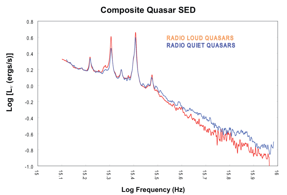
Figure 1: The EUV Deficit. The HST quasar composite continuum accretion disk spectra. The blue and red plots are the ultraviolet SED peak and the EUV composite spectra for RQQs and RLQs, respectively (Telfer et al 2002). Note the steeper SED (larger $\alpha_{\mathrm{EUV}}$) for RLQs.

In the following an extended magnetically arrested scenario is explored (EMAA) in parallel with the analysis of the MAA scenario. In the EMAA model, the magnetic flux that threads the EUV region is the outermost extent of an interior magnetic flux distribution that threads the equatorial plane of the ergosphere and the event horizon of the central supermassive black hole. The one necessary assumption that is required to connect this interior region to observation is that the vertical magnetic flux in the interior region is proportional to the magnetic flux in the EUV region, $\Phi_{int}\propto\Phi_{EUV}$. In this circumstance, the interior magnetic flux distribution is a major source of jet power. The EUV deficit is created by the flux that perforates the innermost accretion flow. Based on the assumption above, this interaction also provides an indirect tracer (a probe with a linear response function) of $\Phi_{int}$. With this assumption, the observational data discussed here also supports the EMAA model.

The paper is structured as follows. The second section is a review of MAA and EUV suppression. In this section, the fundamental relationships between jet power and EUV suppression are found. The goal of this article is to test these predicted relationships versus observations. In order to define the experiment, a method for estimating the jet power from the radio data and a sample of quasars with suitable HST spectra and radio images need to be established. These are the subjects of Sections 3 and 4. Section 5 describes the experimental tests performed and the conclusions. The last section is a discussion of the results.

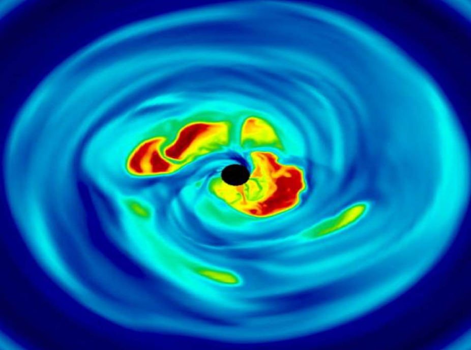
Figure 2: Magnetically Arrested Accretion. The logarithmic false color contour plot of the vertical poloidal magnetic pressure (i.e., $B_{p}=B_{z}$) from an MAA simulation is used to schematically illustrate the concepts posited in this study. One can see Figure 2 of Punsly et al (2009) for the color scale, but this is not necessary for this discussion. The false color accentuates the two-fluid nature of the accretion flow. The red to yellow regions are magnetic islands, the origin of strong Poynting jets and weak EUV emission. The dark blue (the densest plasma) and green are strong EUV emitting regions.

2 Jet Production and Suppressed EUV

The dynamics of viscous shear in black hole accretion flows with and without MAA are reviewed in order to assess the affects of MAA in an annular ring of the accretion flow surrounding the central black hole. Assume that magnetic islands fill a fraction, $f_{V}$, of the volume of the ring, $V$, and penetrate a fraction, $f$, of the top and bottom surface areas of the annular volume, $SA$. The volume of magnetic islands is $V_{MI}$ and its complement in $V$ is $V_{MI}^{C}$, $f_{V}=\int{dV_{MI}}/V$. The surface area elements of the top and bottom faces are, $dS\!A_{MI}$ and $dS\!A_{MI}^{C}$, respectively. The turbulent dissipation that heats the plasma in accretion flows is produced as a consequence of the magneto-rotational instability (MRI) in the 3-D numerical simulations De Villiers et al. (2003); Penna et al (2010). The accretion flow in MAA simulations is perforated by large scale magnetic flux tubes, magnetic islands (see Figure 2). Thus, MAA creates a two component fluid. Firstly, there are regions in which energy is removed from the fluid by turbulent dissipation. Secondly, in the magnetic islands, energy is removed from the flow vertically as Poynting flux (Igumenshchev et al., 2003; Igumenshchev, 2008; McKinney et al., 2012; Tchekhovskoy et al., 2011). The large scale magnetic flux suppresses the MRI induced dissipation in these regions. Simulated MAA flows are subsonic and therefore do not produce significant gas heating from shocks (McKinney et al., 2012; Punsly, 2014). Thus, viscous dissipation is the primary source of heat creation at the boundary of the magnetic islands and in surrounding accreting gas. The total volume available for MRI induced viscous heating is reduced by the magnetic islands. MAA provides an alternative to local turbulent dissipation for removing energy from the plasma allowing the gas to accrete closer to the black hole. The magnetic islands radiate Poynting flux, $S^{P}$, along the magnetic field lines at the expense of the energy of the plasma (Igumenshchev, 2008). The local physics that produces the turbulent viscosity, $\eta_{t}$, in $V_{MI}^{C}$ is unchanged from standard accretion and therefore so is the viscous stress in the fluid surrounding the islands, $T_{r\phi}^{\mathrm{visc}}=\eta_{t}r(d\Omega/dr)$. It was shown in Punsly (2014), in the magnetically arrested case, the radiative luminosity is $\approx 1-f$ of what it would be for standard accretion with the same mass accretion rate. If $f$ is the fraction of the inner accretion flow surface area, $SA$, penetrated by magnetic islands in MAA then the EUV luminosity, $L(\mathrm{EUV})$, obeys the approximate scaling Punsly (2014)

$$L(\mathrm{EUV})\propto(1-f)SA\;.$$ (1)

For any MHD Poynting flux dominated jet, regardless of the source, the total integrated electromagnetic poloidal energy flux is

$$\int{S^{P}\mathrm{d}A_{{}_{\perp}}}=k\frac{\Omega_{F}^{2}\Phi^{2}}{2\pi^{2}c}\;,$$ (2)

where $\Phi$ is the total magnetic flux enclosed within the jet, $\mathrm{d}A_{{}_{\perp}}$ is the cross-sectional area element and $k$ is a geometrical factor that equals 1 for a uniform highly collimated jet (Punsly, 2008). Thus, not only do the magnetic islands of large scale poloidal flux in the inner accretion flow suppress radiation from this region, but they provide a source of Poynting flux (power for the jet) as they orbit around the black hole with an angular velocity, $\Omega_{\mathrm{F}}$. If $M$ is the black hole mass in geometrized units, $\Omega_{F}\sim c/M$ for rotation based on black hole spin or Keplerian orbits. Thus, Equation (2) implies for magnetic islands

$$Q\approx\int S^{P}\mathrm{d}A_{{}_{\perp}}\propto B_{z}^{2}f^{2}\,SA\propto f^{2}P_{\mathrm{ram}}\,SA\ \propto f^{2}\dot{M}(v_{r}/\theta)\;,$$ (3)

where $B_{z}$ is the vertical magnetic field at the disk surface. The string of proportionality statements in Equation (3) require elaboration. The first proportionality arises from the fact that magnetic flux, $\Phi$ is conserved in the perfect magnetohydrodynamic approximation. So the value in the jet is the same as that in the MAA region. In the MAA region $\Phi=\int{B_{z}dS\!A_{MI}}$. This integral is approximated as $\Phi\approx fB_{z}SA$. At this point it is worth reiterating the intent of exploring the EMAA model as well. Equations (2) and (3) can be evaluated using $\Phi\approx\Phi_{int}$ for the jet power, and $\Phi_{int}\propto\Phi_{EUV}\approx fB_{z}SA$. Thus, the following analysis can be used to compare the pure MAA scenario or the EMAA scenario with observation. The only qualification is that the EMAA analysis has the additional assumption that $\Phi_{int}$ scales linearly on average with $\Phi_{EUV}$.

The second proportionality derives from pressure balance at the interface of the magnetic islands and the enveloping accretion flow. In order to evaluate the pressure balance, it is important to realize that the magnetic islands are not frozen into the enveloping accretion flow. For example, in Figure 2 the magnetic islands are in the process of spiraling outward, slowly. The dynamics are not time stationary. Outward motion of the stronger magnetic islands begins in the innermost regions of the accretion flow where the magnetic islands tend to merge (Igumenshchev, 2008). Furthermore, the gas density in the magnetic islands decreases due to outflow (i.e., a jet) in the inner accretion flow. The density is $<1\%$ of the enveloping accretion flow (Igumenshchev, 2008). Hence, they are weakly affected by gravity. By contrast, the dense enveloping accretion flow is strongly attracted to the central black hole. This is a classic Kruskal- Schwarzschild instability, the magnetized version of a Rayleigh-Taylor instability (Stix, 1992). Thus, the magnetic islands become buoyant and drift outward relative to the radial ram pressure of the inflow as discussed in Punsly et al. (2009) and the associated video of a simulated flow. The magnetic field in the islands decreases (expansion and ablation) as they drift outward in response to the decreasing dynamic pressure in an attempt to achieve a new pressure balance with the enveloping medium (Igumenshchev, 2008). This dynamic is unsuccessful and the islands slowly drift outward. In the MAA model considered here, the magnitude of the outward migration velocity, $v_{MI}^{r}$ is much smaller than the magnitude of the bulk radial velocity of the inward enveloping accretion flow, $v_{r}$. This is generally true in the simulations of Igumenshchev (2008), except at the smallest radii where the stronger islands are sometimes particularly unstable and burst outward until a more stable equilibrium is achieved. By contrast, the vertical magnetic flux that permeates the inner accretion flow in the simulation of the Kerr geometry discussed in detail in Punsly et al. (2009); Hawley and Krolik (2006) seems to persist at the smallest radii for longer than it does in the simulations of Igumenshchev (2008), remaining within $r<2M$ (in geometrized units), the ergosphere, for $\sim 2$ local Keplerain orbital periods Punsly (2007). Designate quantities in the magnetic island by the label MI and in the enveloping accretion flow by AF. There are four pressure components, $P_{g}$, $P_{B}$, $P_{r}$, and $P_{\mathrm{ram}}$, corresponding to gas, magnetic, radiation and ram pressure, respectively. $P_{r}$ is a slowly varying quantity around horizontal closed loops in a local neighborhood of the optically thick accretion flow that encircles each magnetic island. The radiation pressure is continuous through the low density magnetic islands. Thus, from the second moment of the radiative transfer equation, one expects $P_{r}(MI)\approx P_{r}(AF)$ at the interface (Punsly, 1996). In the inner accretion flow, $P_{\mathrm{ram}}\gg P_{g}$ in luminous quasars. Unlike $P_{r}$, the ram pressure is not continuous across the boundary, $P_{\mathrm{ram}}(MI)\ll P_{\mathrm{ram}}(AF)$, because of the large density differential and the motion of the magnetic islands relative to the enveloping accretion flow (Punsly, 1996). There is also no buoyancy force in the azimuthal direction. The force on the magnetic islands imposed by the inflow of matter is the strongest force resisting the buoyant outflow of the magnetic islands. Thus, despite all the uncertainty in the precise physics of magnetic island time evolution (see the final section), the radial ram pressure should determine the internal magnetic pressure of the islands to first approximation. Therefore, the pressure balance at the interface of the magnetic island and the enveloping accretion flow is approximately $P_{\mathrm{ram}}(AF)\approx P_{B}(MI)$ (Igumenshchev, 2008). Consequently, the substitution $B_{z}^{2}\propto P_{\mathrm{ram}}$ in Equation (2) was made. In summary, if the magnetic islands are not extremely short-lived transient features in the inner accretion flow, an approximate balance of the ram pressure and the magnetic pressure of the poloidal magnetic field in the islands must exist.

The third proportionality on the right hand side of Equation (2) arises from mass conservation near the black hole, where the “pseudo-half angle”, $\theta$, is the ratio of cross sectional area to $SA$ (evaluated near the outer boundary of the MAA region). Since, as discussed above, $v_{r}-v_{MI}^{r}\approx v_{r}$, to the accuracy of scaling laws in Equation (3), $P_{\mathrm{ram}}\propto v_{r}^{2}$. Consider this in the context of the bolometric luminosity of the accretion disk, $L_{\mathrm{bol}}=\eta(a)\dot{M}c^{2}$, where $\dot{M}c^{2}$ is the mass-energy accretion rate and the accretion efficiency is $\eta(a)$, a function of black hole spin, $a$. Equation (3) can be transformed into an approximate relationship that is more conducive to comparison with observation

$$Q/L_{\mathrm{bol}}\approx C(1/\eta(a))(v_{r}/\theta)f^{2}\;,$$ (4)

where C is a constant. For simplicity, it is assumed that the vast majority of black holes in quasars are rapidly rotating (Bardeen, 1970; Elvis, Risaliti and Zamorani, 2002). Secondly, it is also assumed that variations in $\theta$ and $v_{r}$ provide random scatter to Equation (4) and are not the primary physical drivers of $Q$. It is implicit in the approximate form of Equation (4) that the exact distributions of magnetic islands and the associated functional variation of $\Omega_{F}$ in the magnetically arrested region near the black hole are higher order corrections and only contribute cosmic scatter to the simplified relationship. These approximations are collectively referred to as the homogeneous approximation for the MAA. This makes the following analysis tractable and not dependent of specific models of the various parameters. With these assumptions, Equation (4) and the scaling with $f$ of $L(\mathrm{EUV})$ in Equation (1) implies an approximate relationship,

$$Q/L_{\mathrm{bol}}\approx A(1-L(\mathrm{EUV})/L(\mathrm{EUV})_{\mathrm{RQQ}})^{2}\;,$$ (5)

where A is a constant and $L(\mathrm{EUV})_{\mathrm{RQQ}}$ is the fiducial EUV luminosity if there were no magnetic islands.

3 Long Term Time Averaged Jet Power.

The two most viable options for estimating the jet power, $Q$, of quasars are either based on the low frequency (151 MHz) flux from the radio lobes on 100 kpc scales or models of the broadband Doppler boosted synchrotron and inverse Compton radiation spectra associated with the relativistic parsec scale jet. Each method has its advantage. The 151 MHz method is generally considered more reliable since it does not involve large uncertainties due to Doppler beaming (Willott et al, 1999). A disadvantage is that it involves long term time averages, $\overline{Q}$, that do not necessarily reflect the current state of quasar activity. In this study $Q\equiv\overline{Q}$. A method that allows one to convert 151 MHz flux densities, $F_{151}$ (measured in Jy), into estimates of long term time averaged jet power, $\overline{Q}$, (measured in ergs/s) is captured by the formula derived in Willott et al (1999); Punsly (2005):

$$\overline{Q}\approx[(\mathrm{\textbf{f}}/15)^{3/2}]1.1\times 10^{45}\left[X^{1+\alpha}Z^{2}F_{151}\right]^{0.857}\mathrm{ergs/s}\;,$$ (6)

$$Z\equiv 3.31-(3.65)\times$$

$$\left[X^{4}-0.203X^{3}+0.749X^{2}+0.444X+0.205\right]^{-0.125}\;,$$ (7)

where $X\equiv 1+z$, $F_{151}$ is the total optically thin flux density from the lobes (i.e., contributions from Doppler boosted jets or radio cores are removed). This sophisticated calculation of the jet kinetic luminosity incorporates deviations from the overly simplified minimum energy estimates into a multiplicative factor f that represents the small departures from minimum energy, geometric effects, filling factors, protonic contributions and low frequency cutoff Willott et al (1999). The quantity, f, was further determined to most likely be in the range of 10 to 20 Blundell and Rawlings (2000). In this paper we adopt the following cosmological parameters: $H_{0}$=70 km/s/Mpc, $\Omega_{\Lambda}=0.7$ and $\Omega_{m}=0.3$. Define the radio spectral index, $\alpha$, as $F_{\nu}\propto\nu^{-\alpha}$. The formula is most accurate for large classical double radio sources, thus we do not consider sources with a linear size of less than 20 kpc which are constrained by the ambient pressure of the host galaxy. Alternatively, one can also use the independently derived isotropic estimator in which the lobe energy is primarily inertial in form Punsly (2005)

$$\overline{Q}\approx 5.7\times 10^{44}(1+z)^{1+\alpha}Z^{2}F_{151}\,\mathrm{ergs/sec}\;.$$ (8)

Due to Doppler boosting on kpc scales, core dominated sources with a very bright one sided jet (such as 3C 279 and most blazars) must be treated with care (Punsly, 1995). The best estimate is to take the lobe flux density on the counter-jet side and multiply this value by 2 (bilateral symmetry assumption) and use this estimate for the flux density in Equations (6) - (8).

4 Sample Selection

Determination of quasar EUV continua requires space based observations of modest redshift quasars since ground based observations of high redshift objects in which the EUV is redshifted into the optical are heavily attenuated by the Ly$\alpha$ forrest (Zheng et al., 1997; Telfer, 2002). In order to get a meaningful estimate of $\alpha_{\mathrm{EUV}}$, a range of at least 700 Å  to 1100 Å  in the quasar rest frame is needed to extract the continuum from the numerous broad emission lines (Telfer, 2002). Therefore, a redshift of $z>0.63$ is required. Troughs from Lyman limit systems (LLS) were removed by assuming a single cloud with a $\nu^{-3}$ opacity. This was considered acceptable if the power law above the LLS could be continued smoothly through the corrected region (see the spectra in the Appendix). If there were many strong absorption systems or a LLS that compromised a broad emission line, this simple procedure was deemed inadequate for continuum extraction with the available data and the spectrum was eliminated from the sample. A small correction for the Lyman valley was also made (Zheng et al., 1997). Additionally, if there was evidence of a blazar synchrotron component contribution to the continuum such as a dominant flat spectrum radio core accompanied by high optical polarization or optical/UV variability, or low equivalent width of the emission lines, the underlying accretion disk continuum was considered too uncertain for the sample.

Table 1: The Jet Power of the HST RLQ Sample

Source	Alias	z	Lobe Flux Density	Observed Frequency	Estimated $Q$
			(mJy)	(GHz)	($10^{45}$ ergs/s)
0024+224	…	1.12	11	1.4	$1.38\pm 0.67$
0232-042	PKS 0232-04	1.45	6100	0.178	$32.45\pm 8.81$
0637 -7516	PKS 0637 -752	0.65	209	4.8	$2.83\pm 1.24$
0743-67	PKS 0743-67	1.51	1450	2.5	$65.87\pm 14.4$
0959+6827	…	0.77	27	1.4	$0.27\pm 0.16$
1022+194	4C +19.34	0.83	2400	0.178	$4.01\pm 1.67$
1040+123	3C 245	1.03	1179	1.4	$15.18\pm 4.95$
1137+660	3C 263	0.65	18380	0.151	$13.17\pm 4.42$
1229-021	4C -02.55	1.05	9000	0.160	$20.52\pm 6.25$
1241+176	PG 1241+176	1.27	112	1.4	$2.90\pm 1.27$
1244+324	4C +32.41	0.95	3370	0.151	$6.53\pm 2.51$
1252+119	PKS 1252+119	0.87	15	1.4	$0.31\pm 0.18$
1317+5203	4C+57.21	1.06	3800	0.178	$10.38\pm 3.66$
1340+289	FBQS J1343+2844	0.91	830	0.151	$1.67\pm 0.79$
1340+606	3C 288.1	0.96	9900	0.151	$17.83\pm 5.61$
1354+19	PKS 1354+19	0.72	545	1.4	$3.57\pm 1.32$
1415+172	PKS 1415+172	0.82	1020	0.408	$3.31\pm 1.42$
1857+566	4C +56.28	1.60	8650	0.160	$48.99\pm 11.82$
2149+212	4C +21.59	1.54	5300	0.160	$30.20\pm 8.35$
2340-036	PKS 2340-036	0.90	61	1.4	$0.78\pm 0.41$

Table 2: The EUV Properties of the HST RLQ Sample

Source	Alias	z	$\lambda L_{\lambda}(\lambda=1100\AA)$	$L_{\mathrm{bol}}$	$\alpha_{EUV}$	Spectrograph/
			($10^{45}$ ergs/s)	($10^{45}$ ergs/s)		Grating
0024+224	…	1.12	64,05	243.50	$1.77\pm 0.09$	FOS/G160L
0232-042	PKS 0232-04	1.45	94.47	358.98	$1.75\pm 0.09$	FOS/G160L, G270H
0637 -7516	PKS 0637 -752	0.65	20.80	79.02	$1.75\pm 0.09$	FOS/G160L
0743-67	PKS 0743-67	1.51	110.78	420.95	$2.20\pm 0.30$	FOS/G190H, G270H
0959+6827	…	0.77	22.28	84.65	$1.40\pm 0.10$	FOS/G160L
1022+194	4C +19.34	0.83	7.02	26.67	$2.55\pm 0.15$	FOS/G160L
1040+123	3C 245	1.03	11.90	45.21	$2.20\pm 0.20$	FOS/G160L
1137+660	3C 263	0.65	27.39	104.10	$2.00\pm 0.10$	COS/G130M, G160M; FOS/G190H
1229-021	4C -02.55	1.05	25.09	95.36	$2.65\pm 0.15$	FOS/G160L, G190H, G270H
1241+176	PG 1241+176	1.27	86.78	329.76	$1.79\pm 0.09$	STIS/G230L
1244+324	4C +32.41	0.95	13.77	52.31	$2.41\pm 0.25$	FOS/G160L
1252+119	PKS 1252+119	0.87	16.12	61.27	$1.45\pm 0.10$	FOS/G160L, G190H
1317+5203	4C+57.21	1.06	37.43	142.25	$2.18\pm 0.20$	FOS/G160L
1340+289	FBQS J1343+2844	0.91	14.76	56.08	$190\pm 0.10$	FOS/G160L
1340+606	3C 288.1	0.96	11.39	43.27	$1.78\pm 0.09$	STIS/G140L, G230L
1354+19	PKS 1354+19	0.72	27.46	104.34	$1.95\pm 0.10$	FOS/G160L
1415+172	PKS 1415+172	0.82	7.28	27.66	$1.93\pm 0.10$	FOS/G160L
1857+566	4C +56.28	1.60	22.60	85.87	$2.87\pm 0.14$	STIS/G230L
2149+212	4C +21.59	1.54	18.22	69.24	$2.27\pm 0.20$	STIS/G230L
2340-036	PKS 2340-036	0.90	38.78	147.35	$1.88\pm 0.09$	FOS/G160L

As discussed in the last section, the most reliable methods of estimating the long term time averaged jet power $Q$ are based on the the optically thin emission from relaxed radio lobes. Thus, all sources in the sample needed proof of extended emission on scales larger than the host galaxy so that the lobes can relax ($>20$ kpc). Verification required archival high resolution interferometry images made between 0.408 GHz and 5 GHz. The HST and radio selection criteria resulted in a total of 20 sources for the sample. Note that two new southern hemisphere sources have been added to the sample of spectra from Punsly (2014). The Notes on Individual Sources in the Appendix provides the details that allow these sources to pass the criteria required to be in the sample. The optically thin emission was estimated based on 151 MHz - 178 MHz flux densities (if available) and the lobe fluxes from the radio images. The largest spread in the estimates of $Q$, based on optically thin extended emission, are bounded on the high side by Equation (6) for the parameter, f = 20, and on the low side by Equation (8). These two extremes are used to generate the uncertainty in $Q$ in Table 1.

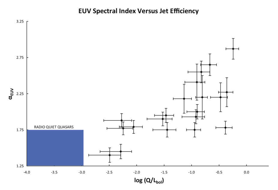
Figure 3: The EUV Deficit versus the Jet Efficiency. A scatter plot of $Q/L_{\mathrm{bol}}$ and $\alpha_{\mathrm{EUV}}$. The blue rectangle represents the RQQs for comparison. The RQQs composite of Figure 1 has $\alpha_{\mathrm{EUV}}=1.57\pm 0.17$ (Telfer et al 2002). Another composite of predominantly RQQs has $\alpha_{\mathrm{EUV}}=1.41\pm 0.16$ (Stevans et al 2014). So a broad range of $1.50\pm 0.25$ is chosen to span both composites.

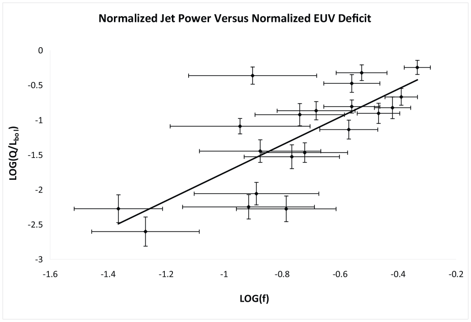
Figure 4: Jet Power and the EUV Deficit. The plot of $\log[Q/L_{\mathrm{bol}}]$, normalized jet power, versus normalized EUV deficit, $\log(f)$. The best fit line is plotted in black for the case that the lower cutoff on $f$ is 0.025. The slope is 2.005 in agreement with the exponent of 2 in Equation (11). The determination of $f$ for small values (flat EUV spectrum sources) is very sensitive to the choice of the fiducial radio quiet EUV level, hence the large error bars for small $f$.

5 Experiment Design and Results

Equations (4) and (5) are two approximate basic and testable predictions of the MAA explanation for the EUV deficit in RLQs. In order to design an experiment to test the validity of the relations, one needs a sample of RLQs with adequate EUV spectra and radio observations to perform the test as described in the last section. Equations (4) and (5) are tested by looking at the HST spectra that cover the span from the SED peak at 1100 Å  to 700 Å . The first experiment tests Equation (4) by assessing the implied correlation between $Q/L_{\mathrm{bol}}$ and $\alpha_{\mathrm{EUV}}$, where the spectral luminosity of the continuum is approximated as $L_{\nu}\propto\nu^{-\alpha_{\mathrm{EUV}}}$. Since the data used here covers the peak of the SED at $\lambda\approx 1100\AA$, an accurate expression, $L_{\mathrm{bol}}\approx 3.8\lambda L_{\lambda}(\lambda=1100\AA)$, can be used to estimate the accretion disk luminosity proper (less reprocessed IR emission in distant molecular clouds) (Davis and Laor, 2011; Punsly, 2014). The relevant data is captured in Tables 1 and 2. The data scatter is plotted in Figure 3. If the MAA scenario is correct not only would there be a correlation between $\alpha_{\mathrm{EUV}}$ with $Q/L_{\mathrm{bol}}$, but the correlation of $\alpha_{\mathrm{EUV}}$ with $Q/L_{\mathrm{bol}}$ should be stronger than $\alpha_{\mathrm{EUV}}$ with $Q$ since dividing by $L_{\mathrm{bol}}$ is equivalent to dividing out the scatter induced by the $B_{z}^{2}$ term in Equation (3). The Spearman rank correlation test indicates that the probability that the correlation of $\alpha_{\mathrm{EUV}}$ and $Q/L_{\mathrm{bol}}$ in Figure 3 occurs by random chance is 0.001. Note this is a more significant correlation compared to a probability of the scatter occurring by random chance of 0.006 for $\alpha_{\mathrm{EUV}}$ and $Q$ and 0.150 for $\alpha_{\mathrm{EUV}}$ and redshift (z). Thus, the expected correlation exists. Physically, the stronger correlation of $Q/L_{\mathrm{bol}}$ with $\alpha_{\mathrm{EUV}}$ compared to $\alpha_{\mathrm{EUV}}$ and $Q$ is evidence that the poloidal magnetic pressure in the islands is being set by the ram pressure of the surrounding accretion flow. The correlation of $Q/L_{\mathrm{bol}}$ with $\alpha_{\mathrm{EUV}}$ is definitely improved, but not dramatically improved from that with $Q$ and $\alpha_{\mathrm{EUV}}$. This is likely a consequence of the circumstance that the correlation with $Q$ is already very strong. Allowing for cosmic scatter generating effects (i.e., a simplified uniform MAA assumption, modest geometric variations from object to object and epoch to epoch within the same object, plus non-contemporaneous measurement of $Q$ with $L(EUV)$), it is probably not realistic to expect that the probability that the correlation of $Q/L_{\mathrm{bol}}$ with $\alpha_{\mathrm{EUV}}$ occurs by random chance is 0 to more than 2 significant digits. In order to see if this is a statistically significant result consider the partial correlation of $Q/L_{\mathrm{bol}}$ with $\alpha_{\mathrm{EUV}}$ when $Q$ is held fixed. The partial correlation coefficient is 0.492 which correspondence to a statistical significance of 0.984. Conversely, the partial correlation of $Q$ with $\alpha_{\mathrm{EUV}}$ when $Q/L_{\mathrm{bol}}$ is held fixed is significant at the 0.581 level. Similarly, repeating this analysis with the Kendall tau rank test, yields: the partial correlation of $Q/L_{\mathrm{bol}}$ with $\alpha_{\mathrm{EUV}}$ when $Q$ is held fixed is statistically significant at the 0.957 level and the partial correlation of $Q$ with $\alpha_{\mathrm{EUV}}$ when $Q/L_{\mathrm{bol}}$ is held fixed is statistically significant at the 0.753 level. There is statistical evidence that the correlation of $Q/L_{\mathrm{bol}}$ with $\alpha_{\mathrm{EUV}}$ is the fundamental correlation and the correlation of $Q$ with $\alpha_{\mathrm{EUV}}$ is a spurious correlation. This supports the premise of equation (3) that it is the jet power divided by accretion rate (ram pressure) that is the physical variable that is related to the EUV deficit. Finally, the much weaker correlation with redshift indicates that more profound physics is occurring, not just cosmic evolution or selection effects.

The second experiment is to test Equation (5) which is much more restrictive than Equation (4) and much more sensitive to any initial assumptions and deviations from the homogeneous approximation. In particular, this experiment will test both the $Q/L_{\mathrm{bol}}$ dependence on $f^{2}$ and the connection between $f$ and the EUV deficit in Equation (1). First, define $L(\mathrm{EUV})$ in a normalized form since from Equation (1) it scales with $SA$. The shortest wavelength that is uniformly sampled is $\lambda=700\AA$, so $L(\mathrm{EUV})\propto L_{\nu}(\lambda=700\AA)$ is the best available proxy for $L(\mathrm{EUV})$. In order to remove the dependence on $SA$ this value is normalized by the peak of the SED

$$L(\mathrm{EUV})\equiv\frac{L_{\nu}(\lambda=700\AA)}{L_{\nu}(\lambda=1100\AA)}\;.$$ (9)

For RQQs, the average value of $\alpha_{\mathrm{EUV}}=1.57\pm 0.17$ from Telfer (2002). As noted in Figure 3, another composite of predominantly intermediate redshift RQQs has $\alpha_{\mathrm{EUV}}=1.41\pm 0.16$ (Stevans et al., 2014). Thus, there is no unique estimate of the fiducial or baseline EUV level for the absence of magnetic islands. The variation in the RQQ EUV translates into an uncertainty in the estimate for $f$ in Equation (5). Denote the maximum and minimum estimates of the EUV in the absence of magnetic islands determined from the HST composite spectral analysis as

$$L(\mathrm{EUV})_{\mathrm{RQQ}}\biggr{|}_{\mathrm{max}}\equiv\frac{L_{\nu}(\lambda=700\AA)}{L_{\nu}(\lambda=1100\AA)}\biggr{|}_{\alpha=1.25}=0.57\;,$$ (10)

$$L(\mathrm{EUV})_{\mathrm{RQQ}}\biggr{|}_{\mathrm{min}}\equiv\frac{L_{\nu}(\lambda=700\AA)}{L_{\nu}(\lambda=1100\AA)}\biggr{|}_{\alpha=1.74}=0.46\;.$$

Combining Equations (5), (9) and (10) yields the crude, but simple prediction of the homogeneous MAA model applied to these intermediate redshift quasars observed with HST,

$$Q/L_{\mathrm{bol}}\approx Af^{2}\approx A\left[1-\left[\frac{L_{\nu}(\lambda=700\AA)}{L_{\nu}(\lambda=1100\AA)}\right]\left[\frac{L_{\nu}(\lambda=1100\AA)}{L_{\nu}(\lambda=700\AA)}\right]\biggr{|}_{\mathrm{RQQ}}\right]^{2}\;.$$ (11)

The larger the estimate for the RQQ EUV baseline level in Equation (10), the larger the value of $f$ (the EUV deficit) that is computed in Equation (11). Equation (11) is utilized as follows in Figure 4 for estimating $f$: the expression for $f$ in Equation (11) is computed two ways, one with the maximum baseline EUV luminosity from Equation (10) and again with the minimum baseline luminosity in Equation (10). The results of these two values in the expression for $f$ in Equation (11) are averaged, this is the $f$ value that is plotted in Figure 4. The uncertainty in this average $f$ is calculated as the maximum of the the expression for $f$ in Equation (11) minus the average. Implementing Equation (10) in Equation (11) is not completely straightforward since according to Table 2, two of the sources have $\alpha_{\mathrm{EUV}}<1.74$ and two others quasars have $\alpha_{\mathrm{EUV}}$ that are close to this value. The volume of the EUV emitting region that is displaced by magnetic islands cannot be negative, $f$ cannot be less than 0 in Equation (11). Thus, consider the example of a lower bound or cutoff of at least $2.5\%$ of the accretion surface area in the EUV region ($f>0.025$) is displaced by magnetic islands for the RLQs with flatter EUV spectrum when the upper limit value of $\alpha_{\mathrm{EUV}}=1.74$ is used in Equation (11) as the condition for the absence of magnetic islands. The result is shown graphically in Figure 4 for each source in Tables 1 and 2. This cutoff is arbitrary, so the effect of its variation is investigated below.

The second experiment in Figure 4 plots the logarithm of $Q/L_{\mathrm{bol}}$ versus logarithm of $f$ from Equation (11) from the data in Tables 1 and 2. The black line is the linear fit to these 20 sources and the slope is 2.01. The theoretical prediction of MAA is 2 in Equation (11). The incredible agreement is clearly coincidental since there is significant scatter and many crude approximations in the derivation of Equation (11). As an illustration of this claim, consider a lower bound of $f>0.05$. In this case, the slope is 2.22. Alternatively, if the lower bound of $f>0.01$ is used, the slope is 1.88. The fit to the best fit line in Figure 4 is fairly good with a squared multiple regression correlation coefficient of 0.57.

6 Implications and Conclusion

The primary results of this study that are presented in Tables 1 and 2 (as well as Figures 3 and 4) are empirical. It was shown that HST EUV spectra and radio interferometry data are consistent with the jet power, $Q$, in RLQs proportional to both the square of the deficit in EUV emission, $f^{2}$, and the accretion rate. The most straightforward interpretation is to assume that magnetic flux tubes occupy a fraction, $f$, of the EUV emitting region since this explains the EUV deficit and jet power connection. Furthermore, it was argued that the MAA/EMAA variants of this idea explains the precise scaling laws that are implied by the observational data. In the following, the experiments designed to test the MAA hypothesis are summarized. The speculative nature of the MAA scenario is critiqued as well as alternative explanations of the observed scaling laws.

In the first experiment, the scatter in Figure 3 indicates that $Q/L_{\mathrm{bol}}$ is strongly correlated with $\alpha_{\mathrm{EUV}}$ as expected from Equation (4), i.e., the jet launching region displaces the EUV emitting region in MAA. Secondly, it was shown that the correlation of $Q/L_{\mathrm{bol}}$ with $\alpha_{\mathrm{EUV}}$ is stronger than the correlation of $Q$ with $\alpha_{\mathrm{EUV}}$. It was argued that this is a statistically significant difference because a partial correlation analysis indicates that the correlation of $Q/L_{\mathrm{bol}}$ with $\alpha_{\mathrm{EUV}}$ is statistically significant and the correlation of $Q$ with $\alpha_{\mathrm{EUV}}$ is spurious. This is evidence of the precise details of MAA that is elucidated by Equation (3), ram pressure regulates the strength of the large scale poloidal field strength in the magnetic islands.

In the second experiment, Figure 4 shows a data scatter that is consistent with the jet strength being proportional to the square of the EUV deficit estimated from HST spectra in RLQs. The fitted slope of the log-log relationships between $Q/L_{\mathrm{bol}}$ and $f$ (Figure 4 is plotted for a lower cutoff $f=0.025$) are consistent with the prediction of Equation (11) of a slope equal to 2. Namely with reasonable variation due to the lower cutoff ($0.01<f<0.05$) the fitted slope was found to be $2.05\pm 0.17$. This is significant evidence that the fundamental details of the crude MAA model are consistent with the observations. Figure 4 indicates that $f$ is a few percent for the RLQs with weaker jets and $\sim 40\%$ for the RLQs with the most powerful jets.

It is not claimed that this is the only possible explanation of the EUV deficit in RLQs. Other explanations based on numerical and theoretical models include, lower $a$ in RLQs (larger innermost stable orbit), or stronger quenching winds in RLQs per the model of Laor and Davis (2014). Note that a scenario of larger black hole mass and lower accretion rates in RLQs was ruled out empirically as a plausible explanation due to the indistinguishable SED peak in RLQs and RQQs (Punsly, 2014). However, none of these other explanations naturally produces a radio jet and the correlation in Figure 3.

Furthermore, it is also not claimed that this is the only possible explanation of $Q$ being controlled by $P_{\mathrm{ram}}$. Magnetic flux pinned to the event horizon as in McKinney et al. (2012); Tchekhovskoy et al. (2011) or trapped in an equatorial gap between the accretion flow and the black hole as in Punsly (2008) would also result in this same correlation. However, neither of these scenarios explain the $Q/L_{\mathrm{bol}}$ scaling with the square of the EUV deficit, $f^{2}$ found in Figure 4. A possible reconciliation is provided near the end of this section.

In Section 2, it was noted that “if the magnetic islands are not extremely short-lived transient features in the inner accretion flow, an approximate balance of the ram pressure and the magnetic pressure of the poloidal magnetic field in the islands must exist.” Currently, the diffusion rate of plasma onto and off of magnetic field lines and magnetic reconnection rates are not well known near black holes. Not only are these issues critical for the formation of the magnetic islands, but the time evolution of the magnetic islands is determined primarily by diffusion (Igumenshchev, 2008; Punsly, 2015). These dynamical elements only occur as a consequence numerical diffusion in modern simulations in over simplified ideal MHD single fluid models of the physics (Punsly, 2015). It is not even clear theoretically what the basic principles required for an accurate physical depiction would be. Many issues that are related to these topics are active areas of investigation in solar and fusion physics (Bauman et al, 2013; Malakit, 2009; Threlfall et al., 2012; Yamada, 2007). As such, it cannot currently be claimed or refuted that long-lived magnetic islands can or cannot exist in the inner accretion flow. The magnetic islands should become Kruskal- Schwarzschild unstable if the density becomes low enough and should move outward, not inward. A key physical element is the numerical approximation of the physics that determines the density. If the numerical diffusion is significant, low enough density may not be achieved before the flux tubes are dragged across the event horizon. The simulations in Igumenshchev (2008); Punsly et al. (2009) indicate a population of magnetic islands within the innermost accretion flow consistent with the range of filling factors, $f$, that are found in Figure 4. In the innermost accretion flow, the time evolution of the islands is non-steady. The inner accretion flow is a dynamic region. There are epochs with very few magnetic islands and epochs in which the (large) magnetic islands near the black hole become buoyant after losing mass to the jet and slowly wind their way out against the ram pressure of the accretion flow. By contrast, the simulations in McKinney et al. (2012); Tchekhovskoy et al. (2011, 2012) that are heavily seeded with large scale magnetic flux are devoid of magnetic islands close to the event horizon. This is evidenced by the claim in McKinney et al. (2012) that no significant Poynting flux emerges from this region (see Equation 2, above) as well as the linked online videos of the simulations. The videos show the innermost significant, modest, magnetic island concentrations are located at $r>10M$ and they are extremely transient. Thus, even though the simulations in McKinney et al. (2012); Tchekhovskoy et al. (2011, 2012) have strong Poynting jets from the event horizon, they are not consistent with the EMAA model. This either means that the interpretation of the EUV deficit presented here is wrong or the simulations do not represent the magnetic flux evolution accurately. The latter option is favored empirically, since magnetic flux displacing EUV emitting gas in the inner accretion flow explains two correlated phenomena, jet power and the EUV deficit. It not only explains the correlation, but it predicts the explicit scaling laws for jet power with accretion rate and with the degree of EUV suppression implied by the observations. The simulations without significant vertical magnetic flux in the innermost accretion flow explain only the scaling law for jet power with accretion rate.

Recall the fact that the only difference between the RLQ and RQQ composite continua in Figure 1 is the EUV. Comparing this difference to numerical simulations indicates that the magnetic islands are concentrated between the event horizon and an outer boundary of $<2.8M$ (in geometrized units) for rapidly rotating black holes (Punsly, 2014; Penna et al, 2010). Thus the simple, homogeneous MAA model does not preclude a black hole spin assisted component that displaces the EUV emitting gas inside $r<2M$ as in the ”erogspheric disk” that has been found to occur in some 3-D numerical simulations of high spin black holes (Punsly, 2008; Punsly et al., 2009). It is also possible that a certain fraction of the flux distribution in the inner accretion flow threads the event horizon and extracts spin energy (Blandford and Znajek, 1977). In particular, what is shown here is that a significant magnetic flux in the inner accretion flow (based on Figure 4 from 2.5% to 45% of the EUV emitting region in RLQs is filled with magnetic islands) explains the EUV deficit and the source of the jet power is proportional to the square of this putative flux. However, the distribution of flux can be larger than just the inner accretion flow. For example, the magnetic flux distribution might in general thread the horizon and the ergospheric equatorial plane as well. This is the EMAA model that was sketched out in the introduction. The magnetic islands in the innermost accretion flow would represent the outermost portion of this flux distribution in this scenario. This inner region of magnetic flux would be proportional to the flux that threads the EUV region for the putative generic flux distribution, $\Phi_{int}\propto\Phi_{EUV}$. The power from the event horizon jet and/or the ergospheric disk jet could be larger than the jet power from the EUV region. In this scenario, the flux in the innermost accretion flow is merely a “tracer” for flux contained in these interior regions and not coincident with the primary source of the Poynting flux that powers the jet. However, the flux permeating the innermost accretion flow must be significant and the flux in these interior regions is presumed to scale with that in the EUV region. Namely, from Figure 4, for a weak jet like that in PKS 1252+119, $f\sim 4\%$ and for a strong jet like that of 1857+566 $f\sim 45\%$. By the EMAA assumption, one would expect the event horizon/ergosphere flux to be $\sim 10$ times larger in 1857+566 compared to PKS 1252+119 on average (and therefore $Q/L_{\mathrm{bol}}$ $\sim 100$ times larger) in order to explain the observational results (Figures 3 and 4) that are described in this paper. The implication is still that simulations of jets from these regions would need to have a significant flux in the innermost accretion flow to be consistent with the observations. As with the discussion of the time evolution of magnetic islands above, the existing numerical algorithms are single fluid MHD approximations to the physics in which numerical diffusion determines reconnection rates and diffusion rates and may not be reliable depictions of the physical model of magnetic field dynamics in the innermost accretion flow near black holes. As such, a different mathematical description of the reconnection process can lead to very different poloidal magnetic flux distributions near the black hole (Punsly, 2015). Hence, much of this discussion is speculative. On a less speculative note, the fundamental deduction drawn from the EUV observations is that future modeling and theory of quasar jet origins should contain the feature of an innermost accretion flow threaded by substantial vertical magnetic flux.

It is necessary for a critical analysis that one segregates the various issues addressed in the MAA/EMAA model and the numerical simulations by the degree to which they have been verified by the scientific method, observation. The hierarchal list below is in order of the degree to which each of these issues is verified by observations.

1. EUV deficit and radio loudness: The EUV deficit is verified observationally here and in Punsly (2014) to correlate with low frequency radio luminosity on super-galactic scales (converted to jet power here in order to make contact with theoretical treatments).

2. EUV originates from inner accretion flow: Being on the high frequency tail of the optically thick thermal spectrum this is the obvious interpretation. However, observational verification is scientifically much more robust. The only direct method of estimating the size of the EUV region is through time variability arguments. This requires the ability to collect a significant EUV flux on short time scales. The only reasonable set of observations related to an active nucleus are the EUVE (Extreme Ultraviolet Explorer) observations of NGC 5548. Simultaneous UV and EUV monitoring indicated that the most likely interpretation of the EUV emission was the Wien tail of the optically thick thermal emission and it had significant variability (Marshall et al., 1997). Further EUV monitoring found significant variability at the smallest sampling time scales $t_{var}<5600$ s (Haba et al, 2003). Standard arguments based on the light travel time across the EUV emitting region and black hole reverberation mass estimates of the central black hole indicate the EUV emitting gas is located in a volume with a radius, $r<10.5$M (Bentz et al., 2007; Denney et al,, 2010). The light curve in Haba et al (2003) seems to indicate that with a higher sensitivity telescope, the time scale for variability would likely be less than 5600 s. This is observational evidence that the EUV is radiated from the innermost accretion flow.

3. The only know energy source for the extreme powers in relativistic quasar jets is Poynting flux (independent of the details of its origins) and this scales with the square of the enclosed poloidal magnetic flux.

4. Magnetically arrested accretion occurs in some numerical models, however the dynamics of the arresting magnetic flux tubes differs from what is indicated in the MAA/EMAA model to varying degrees. The difference is small to modest in Igumenshchev (2008); Punsly et al. (2009), that agree with the fill fraction, $f$, expected from Figure 4 in the innermost accretion flow. The time evolution generally agrees with the MAA/EMAA model except that some of the islands may not agree due to some very unstable magnetic outbursts at the smallest radii. The difference from the MAA/EMAA explanation of the observations is large in McKinney et al. (2012); Tchekhovskoy et al. (2011, 2012) for which fill fraction, $f\approx 0$ in the innermost accretion flow. The “magnetically choked accretion flows” of McKinney et al. (2012) heat the innermost accretion flow compressively as part of the magnetic choking process. This likely eliminates the EUV region by drastically elevating the temperature of the innermost accretion flow as opposed to suppressing the emission from the innermost accretion flow as the observations indicate. Alternatively, depending on the precise, unknown, details of radiative transfer in this hot, dense gas, the compressive heating might drastically harden the high frequency tail of the optically thick spectrum in RLQs, the opposite of what is observed.

This list is the basis of the logic of the analysis presented in this study. Items 1 and 2 above state that observations directly indicate that jets disrupt (suppress) the EUV emission from the inner accretion disk and the amount of disruption scales with the power of the jet. The third point states that the only known mechanism for driving such a powerful relativistic jet is Poynting flux that requires significant poloidal magnetic flux at its source. Thus, with very little speculation, it is indicated that both the large scale poloidal magnetic flux at the base of the jet and a mechanism that suppresses (but does not eliminate) the EUV emission from the innermost accretion flow coexist at the heart of the central engine of RLQs. The main assumption of the MAA/EMAA idea is that this is too large of a coincidence, some of this magnetic flux must be the same element that disrupts, but does not eliminate the innermost accretion flow. If a numerical effort cannot reproduce this circumstance then perhaps the numerical approximation to the relevant physical processes requires further development. Observations should lead the numerical work.

Appendix 1.: Notes on Individual Sources

0024+224. The NVSS image at 1.4 GHz shows a predominantly core-jet morphology. The one-sided jet is likely Doppler boosted kpc emission as is typical of most RLQs viewed close to the jet axis Punsly (1995). There are two faint flux density peaks just beyond the hot spot at the end of the jet. This is taken as evidence of isotropic halo type emission and this flux density is used in the estimate of Q. Even though the radio source is core-dominated, the optical polarization and optical variability are small and the emission lines have high equivalent widths, Thus, Doppler boosted jet emission in the EUV is considered negligible.

0232-042. This is a strong lobe dominated source, so the low frequency total flux density at 178 MHz is the best estimator for Q.

0637-752. This is a famous core plus one-sided kpc jet dominated southern hemisphere radio source. There is clearly considerable Doppler beaming. The most reliable estimate of isotropic flux is to take twice the counter lobe flux density as discussed above. This is attained from the ATCA 4.8 GHz radio image Tingay et al (1998). Even though the radio source is core-dominated, the optical polarization and variability are small and the emission lines have high equivalent widths, Thus, Doppler boosted jet emission in the EUV is considered negligible.

0743-67. This is one of the most intrinsically luminous quasars and is also a very strong radio source, both the radio core and the lobes. The lobe flux density is estimated from ATCA radio observations Punsly and Tingay (2005). Even though the radio core exceeds 1 Jy, the optical polarization and variability are small and the emission lines have high equivalent widths, Thus, Doppler boosted jet emission in the EUV is considered negligible. This source has significantly higher visual extinction than any other source in the sample, $A_{V}$ = 0.362. Thus, unlike the other sources, the detailed form of the Galactic extinction law significantly affects the EUV continuum fit. The average Galactic value of $R_{V}$ = 3.1, gives a poor fit to a power-law continuum for the CCM model Cardelli et al. (1989). The reason is clear, de-convolving the extinction due to the $\lambda 2175$ bump has created an “artificial” kink in the spectrum presented in this Appendix (this equates to 865 Å  rest frame). A larger value of $R_{V}$ will remove this artificial bend and these values have been found for various lines of sight in the Galaxy Cardelli et al. (1989). Using $R_{V}$ = 4.5 or $R_{V}$ = 5.5 makes the continuum look more like a power-law in the spectra above. Even though the largest value of $R_{V}$ gives the smoothest continuum fit, and improves the scatter plots in Figures 3 and 4, a conservative intermediate choice is taken with a large uncertainty assigned in Table 2.

0959+6827. Fortunately, this weak radio source was observed the VLA Landt et al. (2006). This is a triple radio source. Such weak sources are very rarely imaged with high resolution VLA (as is required at intermediate and high redshift in order to resolve most radio sources).

1022+194. This source has a strong core (480 mJy) and a large amount of diffuse, elongated emission (160 mJy) at 1.4 GHz in FIRST images. The core spectrum is flat from 1.4 GHz to 5 GHz Hutchings et al. (1988). The total spectrum is very steep at low frequency, so it seems that the diffuse extended emission dominates at 178 MHz. Thus, the total 178 MHz flux density is used in the estimate of Q.

1040+123. 3C 245 is the rare quasar with a 1 Jy radio core and very strong symmetric radio lobes. In order to get a good estimate of Q, a high resolution radio map is needed to extract the radio core and jetted emission Murphy et al. (1993). Even though the radio core exceeds 1 Jy, the optical polarization and variability are small and the emission lines have large equivalent widths, Thus, Doppler boosted jet emission in the EUV is considered negligible.

1137+660. 3C 263 is a lobe dominated quasar, so the low frequency total flux density at 151 MHz is the best estimator for Q.

1229-021. This is a classical triple that is steep spectrum at low frequency. Thus, the 160 MHz flux density is used to estimate Q. This is a low optical polarization quasar with modest optical variability and the emission lines have large equivalent widths. It is concluded that the continuum in the EUV is dominated by the optically thick thermal emission. This is corroborated by negligible changes in the EUV continuum between HST observations separated by more than 2 years.

1241+176. A faint, very distant secondary is connected to the radio core by a thin bridge in the 5 GHz radio image Kellerman et al. (1994). The flux density of this component as determined by the NVSS image at 1.4 GHz is used to estimate Q. HST observations separated by 9 years show negligible EUV variability. This combined with large emission line equivalent widths indicate that the radio core does not contribute significantly to the EUV continuum.

1244+324. This is a classical triple, lobe dominated radio source. Thus, the 151 MHz data is used to estimate Q.

1252+119. This is a core dominated radio source with a weak jet. However, the 1.4 GHz radio image shows diffuse emission beyond the end of the jet that is considered evidence of a core-halo type source Price et al. (1993). The faint extension is used to estimate the halo (lobe) flux density for use in the computation of Q. This is a low optical polarization source that is not highly variable in the optical. There is no EUV variability over a 4 year span of HST observations. Thus, it is concluded that even though the source is core dominated, the relativistic jet contributes negligibly to the EUV.

1340+289. At 1.4 GHz, the flux is equally split between a “core” and the southern lobe Hutchings et al. (1988). The 4.8 GHz image shows a small northern extension, likely part of a lobe emission. The overall size is at least 25 kpc at 4.8 GHz making it suitable for this sample and the estimation techniques for Q Price et al. (1993). The spectrum is steep at low frequency, so it is assumed that the lobe emission dominates the 151 MHz flux density and this is used to estimate Q. The optical polarization is low and there is no evidence of strong optical variability. Combined with the large equivalent widths of the emission lines implies that there is very little synchrotron contamination of the EUV continuum.

1340+606. 3C 288.1 is a lobe dominated radio source, so the 151 MHz flux density is used to estimate Q.

1354+19. This source has a strong radio core and a strong one-sided jet, similar to PKS 0637 -752. Since the counter-lobe is more luminous than the lobe on the jetted side in the 1.4 GHz high resolution radio images, it is safe to assume that Doppler beaming is insignificant in the jetted lobe Murphy et al. (1993). Thus, the total lobe flux density at 1.4 GHz (less the Doppler beamed one - sided kpc jet emission) is used to compute Q. This object has low optical polarization and is mildly variable in the optical. Comparing the G160L and G270H spectra taken 14 months apart, there is no difference in the overlap region, thus the rest frame far UV flux is not highly variable. Thus, it is concluded, in spite of the strong radio core, that the EUV is predominantly optically thick thermal emission.

1415+172. This is a lobe dominated triple Hutchings et al. (1988). Thus, the total low frequency flux density is used to estimate Q.

1857+566. This is a powerful steep spectrum triple Barthel et al. (1988). Thus, the low frequency total flux density is used for estimating Q.

2149+212. This is a compact ($20$ kpc) steep spectrum triple Barthel et al. (1988). Thus, the low frequency total flux density is used for estimating Q.

2340-036. This source is a symmetric core dominated triple radio source in FIRST images. The 1.4 GHz flux density of the lobes is extracted from the FIRST data and is used in the computation of Q. Even though the radio source is core-dominated., the optical polarization and variability are small and the emission lines have high equivalent width, Thus, Doppler boosted jet emission in the EUV is considered negligible.

Appendix 2.: HST Spectra

Figure 5 are the EUV spectra corrected for Galactic extinction, the Lyman $\alpha$ forest and Lyman limit systems as discussed in the Sample Selection section. The spectra are arranged in order of increasing $Q/L_{\mathrm{bol}}$ in order to see the trend of increasing EUV deficit regardless of the precise continuum power law fits (the black lines). The spectra are log-log plots of $F_{\lambda}$ as a function of $\lambda$. The data was downloaded from MAST and smoothed as required to enhance the definition of the continuum

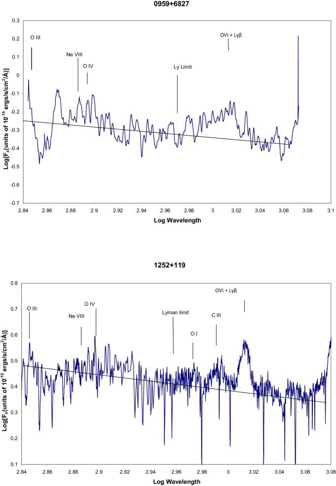
Figure 5: a

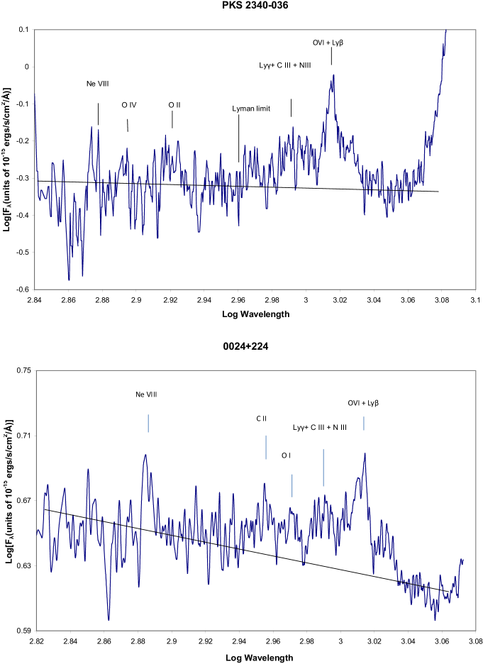
Figure 5: b

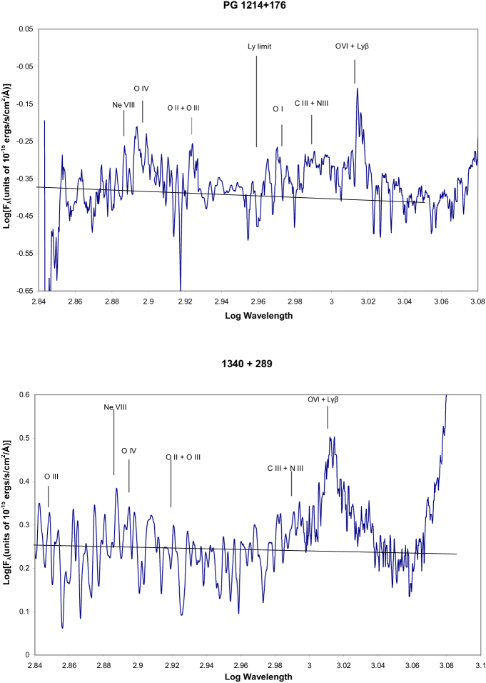
Figure 5: c

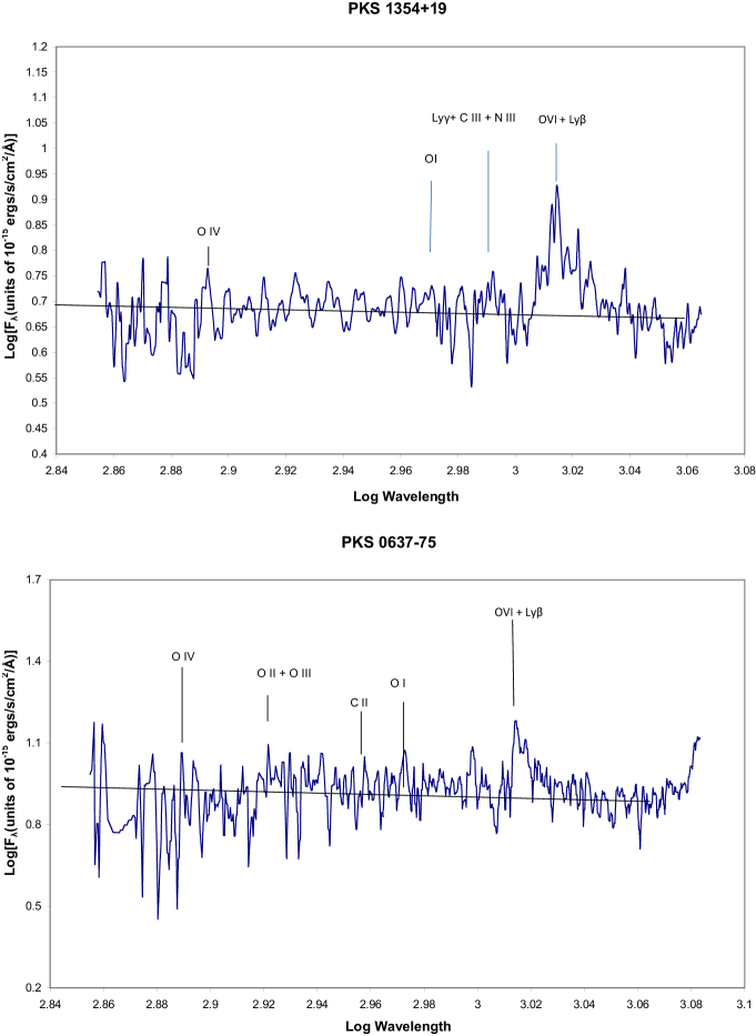
Figure 5: d

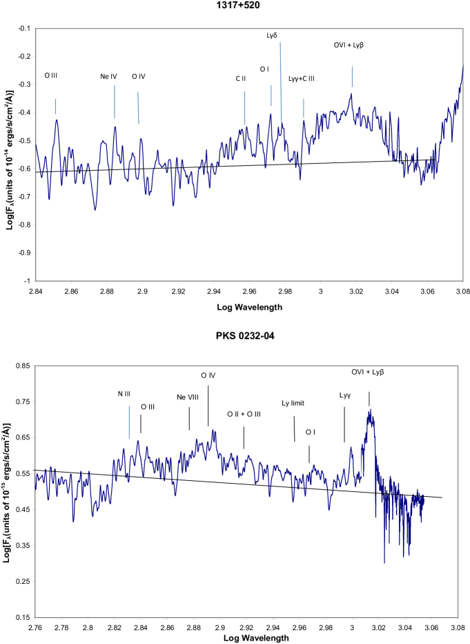
Figure 5: e

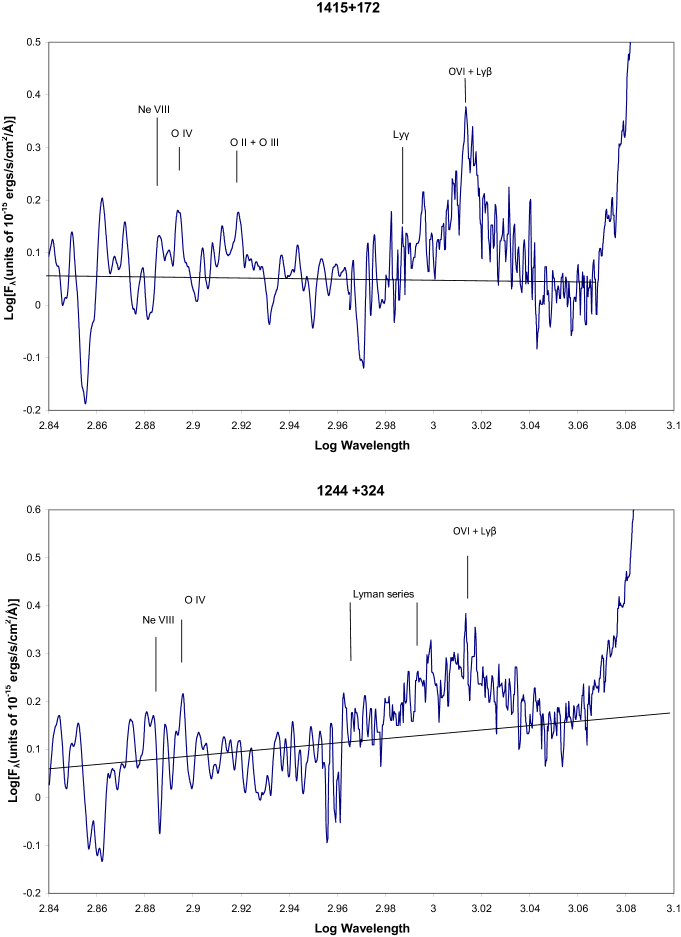
Figure 5: f

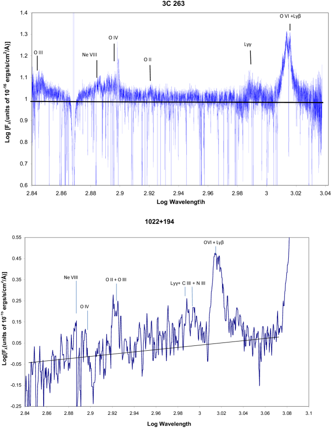
Figure 5: g. The spectral data for 3C 263 was generously provided by Michael Shull and Matt Stevans

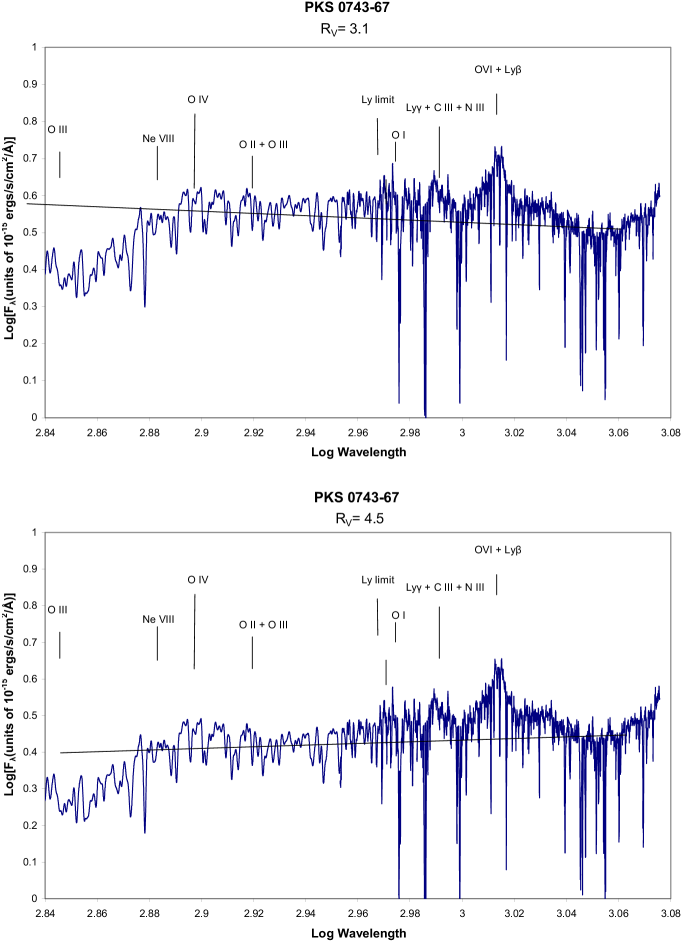
Figure 5: h.

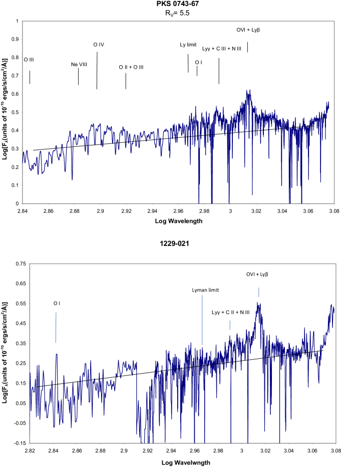
Figure 5: i.

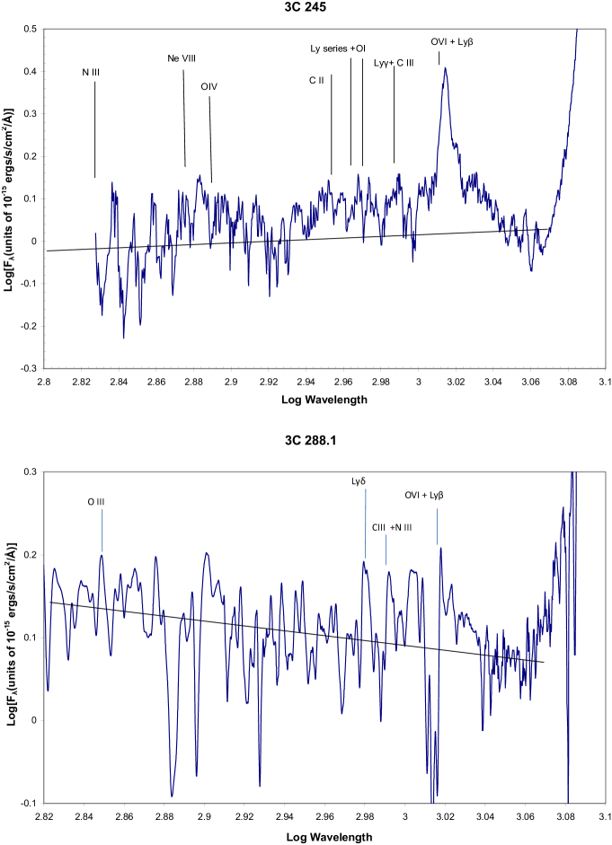
Figure 5: j.

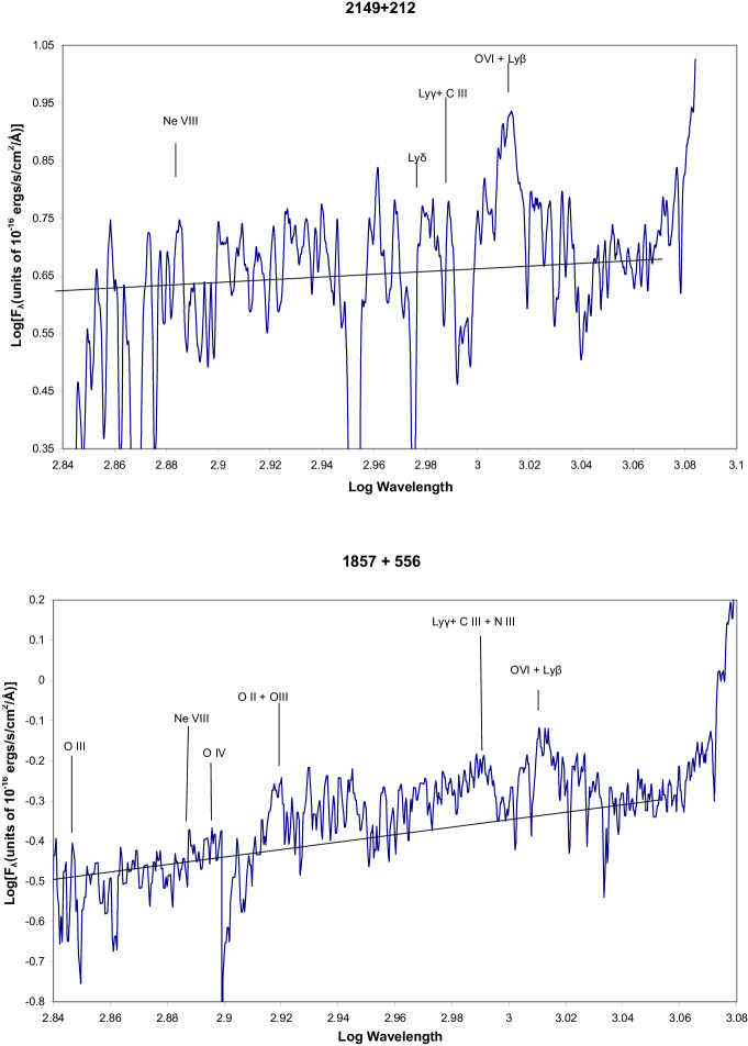
Figure 5: k.

References

- Bardeen (1970) Bardeen, J. 1970 Nature 226 64
- Barthel et al. (1988) Barthel, P. D., Miley, G. K., Schilizzi, R. T., Lonsdale, C. J. 1988 Astron. & Astrophys. Supp. 73 515
- Bauman et al (2013) Baumann, G., Galsgaard, K. & Norlund, A., 2013 Solar Physics 284 467
- Bentz et al. (2007) Bentz, M. et al. 2007 ApJ 662 205
- Blandford and Znajek (1977) Blandford, R. and Znajek, R. 1977 MNRAS 179 433
- Blandford and Payne (1982) Blandford, R. D. and Payne,D., 1982 MNRAS 199 883
- Blundell and Rawlings (2000) Blundell, K., Rawlings, S. 2000 AJ 119 1111
- Boroson and Green (1992) Boroson, T. and Green, R. 1992 ApJS 80 109
- Brotherton et al. (1994) Brotherton, M., Wills, B. Steidel, C. and Sargent, W. 1994 ApJ 423 131
- Cardelli et al. (1989) Cardelli, J., Clayton, G., Mathis, J. 1989 ApJ 345 245
- Davis and Laor (2011) Davis, S., Laor, A. 2011, ApJ 728 98
- Denney et al, (2010) Denney, K. et al 2010, ApJ 721 715
- De Villiers et al. (2003) De Villiers, J-P., Hawley, J., Krolik, 2003 ApJ 599 1238
- Elvis, Risaliti and Zamorani (2002) Elvis, M., Risaliti, G., Zamorani, G. 2002 ApJ L565 75
- Haba et al (2003) Haba et al. 2003, ApJ 599 949
- Hawley and Krolik (2006) Hawley, J., Krolik, K. 2006, ApJ 641 103
- Hutchings et al. (1988) Hutchings, J., Price, E., Gower, A.. 1988 ApJ 329 122
- Igumenshchev et al. (2003) Igumenshchev, I. V., Narayan, R. and Abramowicz, M. A. 2003 ApJ 592 1042
- Igumenshchev (2008) Igumenshchev, I. V. 2008 ApJ 677 317
- Kellerman et al. (1994) Kellerman et al. 1994 AJ108 1163
- Landt et al. (2006) Landt, H., Perlman, E., Padovanni, P.. 2006 ApJ 637 183
- Laor and Davis (2014) Laor, A., Davis, S. 2014 ApJ 428 3024
- Lind and Blandford (1985) Lind, K., Blandford, R.1985 ApJ 295 358
- Lovelace (1976) Lovelace, R. V. E. 1976 Nature 262 649
- Lynden-Bell and Rees (1971) Lynden-Bell, D., Rees, M. 1971, Mon. Not. R. Astr. Soc. Lett. 152 461
- Malakit (2009) Malakit, K., Cassak, P., Shav, M., Drake, F. 2009, Geosphysical Research Letter 36 L07107
- Malkan (1983) Malkan, M. 1983, ApJ 268, 582
- Marshall et al. (1997) Marhall, H. 1997, ApJ 479, 222
- McKinney et al. (2012) McKinney, J., Tchekhovskoy, A., Blandford, R. 2012 MNRAS 423 3083
- Meier (1999) Meier, D. L. 1999, ApJ 522, 753
- Murphy et al. (1993) Murphy, D., Browne, I.W.A., Perley, R.. 1993 MNRAS 264 298
- Novikov and Thorne (1976) Novikov, I. and Thorne, K. 1973, in Black Holes: Les Astres Occlus, eds. C. de Witt and B. de Witt (Gordon and Breach, New York), 344
- Penna et al (2010) Penna, R. et al 2010 MNRAS 408 752
- Price et al. (1993) Price, E., Gower, A..Hutchings, J., Talon, S., Duncan D., Ross, G. 1993 ApJS 86 365
- Punsly (1995) Punsly, B. 1995 AJ 109 1555
- Punsly (1996) Punsly, B. 1996 ApJ 473 178
- Punsly (2008) Punsly, B. 2008, Black Hole Gravitohydromagnetics, second edition (Springer-Verlag, New York)
- Punsly (2005) Punsly, B. 2005 ApJL 623 9
- Punsly (2007) Punsly, B. 2007, MNRAS Letters 381,79
- Punsly (2014) Punsly, B. 2014 ApJL 797 33
- Punsly (2015) Punsly, B. 2015 The Formation and Disruption of Black Hole Jets, ASSL, 414 ISBN 978-3-319-10355-6. Springer International Publishing Switzerland, p. 149
- Punsly et al. (2009) Punsly, B., Igumenshchev, I. V., Hirose, S. 2009 ApJ 704 1065
- Punsly and Tingay (2005) Punsly, B., Tingay, S. 2005 ApJL 633 89
- Shakura and Sunyaev (1973) Shakura, N., Sunyaev, R. 1973, A & A 24 337
- Steidel and Sargent (1991) Steidel, C. and Sargent, W. 1991 ApJ 383 433
- Stevans et al. (2014) Stevans, M., Shull, M., Danforth, C., Tilton, E. 2014ApJ 794 75
- Stix (1992) Stix, T. Waves in Plasmas.(American Institute of Physics, New York, 1992)
- Szuszkiewicz et al. (1996) Szuszkiewicz, E., Malkan, A., and Abramowicz, M. A. 1996 ApJ 458 474
- Tchekhovskoy et al. (2011) Tchekhovskoy, A., Narayan, R. and McKinney, J. 2011 MNRAS Lett. 418 79
- Tchekhovskoy et al. (2012) Tchekhovskoy, A.,McKinney, J. 2012, MNRAS Letters 423 55
- Telfer (2002) Telfer, R., Zheng, W., Kriss, G., Davidsen, A. 2002 ApJ 565 773
- Threlfall et al. (2012) Threlfall, J. et al 2012, A & A 544 24
- Tingay et al (1998) Tingay, S. et al. 1998 ApJL 497 594
- Willott et al (1999) Willott, C., Rawlings, S., Blundell, K., Lacy, M. 1999 MNRAS 309 1017
- Yamada (2007) Yamada, M.2007, Physics of Plasmas 14 058102
- Zheng et al. (1997) Zheng, W. et al. 1997 ApJ 475 469
- Zhu et al. (2012) Zhu, Y. et al. 2012, MNRAS 424 2504