Diffuse approximation to the kinetic theory in a Fermi system

Abstract

We suggest the diffuse approach to the relaxation processes within the kinetic theory for the Wigner distribution function. The diffusion and drift coefficients are evaluated taking into consideration the interparticle collisions on the distorted Fermi surface. Using the finite range interaction, we show that the momentum dependence of the diffuse coefficient $D_{p}(p)$ has a maximum at Fermi momentum $p=p_{F}$ whereas the drift coefficient $K_{p}(p)$ is negative and reaches a minimum at $p\approx p_{F}$. For a cold Fermi system the diffusion coefficient takes the non-zero value which is caused by the relaxation on the distorted Fermi-surface at temperature $T=0$. The numerical solution of the diffusion equation was performed for the particle-hole excitation in a nucleus with $A=16$. The evaluated relaxation time $\tau_{r}\approx 8.3\cdot 10^{-23}\mathrm{s}$ is close to the corresponding result in a nuclear Fermi-liquid obtained within the kinetic theory.

I Introduction

The relaxation processes in many-body systems can be effectively studied within the kinetic theory, see Ref. kosh04  and references therein. The kinetic approaches operate with the kinetic equation, which is written for the distribution function in phase space. The advantage of the kinetic approaches is that the kinetic equation can be easily generalized to the case of finite temperatures. Certain difficulties arise when one tries to describe the relaxation and damping effects involving the collision integral in $9$-dimension space bert78 ; kopl95 ; mako95 ; kiko96 ; kopl96 ; diko99 .

To reduce the kinetic equation for the Wigner distribution function, we will follow the diffuse approach lipi81 considering the relaxation on the distorted Fermi surface. The presence of the Fermi-surface distortion effects gives rise to some important consequences. Because of the Fermi-surface distortion, the scattering of particles leads to the relaxation and the damping. The purpose of present paper is to study the diffusion and drift terms in a Fermi-system which can be applied to the description of the damping of collective and particle-hole excitations as well as the large amplitude dynamics. In Sec. 2 we consider the kinetic equation for the Wigner distribution function and reduce it applying the diffusion approximation. In Sec. 3 we establish the diffusion and drift coefficients taking into consideration the Fermi-surface distortion effects. The discussion of numerical results is presented in Sec. 4. Our conclusions are given in Sec. 5.

II Collision integral within diffuse approximation

We will restrict ourselves to the Born collision approximation in the kinetic equation for Wigner distribution function $f(\mathbf{r},\mathbf{p};t)\equiv f$ kaba62 ; risc80 . Introducing the collision integral $\mathrm{St}\{f\}$, we will write the kinetic equation as

$${\frac{\partial f(\mathbf{r},\mathbf{p}_{1};t)}{\partial t}}+\hat{L}f(\mathbf{r},\mathbf{p}_{1};t)=\mathrm{St}\{f\},$$ (1)

where $\hat{L}$  is the driving operator. In the lowest order in $\hbar$ the driving operator $\hat{L}$ is given by kosh04

$$\hat{L}={\frac{1}{m}}\,\mathbf{p}\cdot\mathbf{\nabla}_{\mathbf{r}}-(\mathbf{\nabla}_{\mathbf{r}}U)\cdot\mathbf{\nabla}_{\mathbf{p}}.$$ (2)

Here, the single-particle potential $U$ includes, in general, the self-consistent and external fields. The collision integral $\mathrm{St}\{f\}$ in Eq. (1) can be written in the following form abkh59

$$\mathrm{St}\{f\} = \int\frac{g^{2}d\mathbf{p}_{2}d\mathbf{p}_{3}d\mathbf{p}_{4}}{(2\pi\hbar)^{6}}\ \mathcal{W}(\{\mathbf{p}_{j}\})$$ (3)

$$\times\left[\tilde{f}(\mathbf{p}_{1})\tilde{f}(\mathbf{p}_{2})f(\mathbf{p}_{3})f(\mathbf{p}_{4})-f(\mathbf{p}_{1})f(\mathbf{p}_{2})\tilde{f}(\mathbf{p}_{3})\tilde{f}(\mathbf{p}_{4})\right]\delta(\Delta\varepsilon)\delta(\Delta\mathbf{p})$$

$$= \int\frac{gd\mathbf{p}_{3}}{(2\pi\hbar)^{3}}\ \left[W_{3\rightarrow 1}(\mathbf{p}_{1},\mathbf{p}_{3})\tilde{f}(\mathbf{p}_{1})f(\mathbf{p}_{3})-W_{1\rightarrow 3}(\mathbf{p}_{1},\mathbf{p}_{3})f(\mathbf{p}_{1})\tilde{f}(\mathbf{p}_{3})\right],$$

where $g$ is the spin-isospin degeneracy factor, $\ f(\mathbf{p})\equiv f(\mathbf{r},\mathbf{p},t)$, $\tilde{f}(\mathbf{p})=1-f(\mathbf{p})$, $\Delta\varepsilon=\varepsilon_{1}+\varepsilon_{2}-\varepsilon_{3}-\varepsilon_{4},$ $\Delta\mathbf{p}=\mathbf{p}_{1}+\mathbf{p}_{2}-\mathbf{p}_{3}-\mathbf{p}_{4}$ and $\mathcal{W}(\{\mathbf{p}_{j}\})$ is the probability of two-body collisions. The gain and loss terms $W_{3\leftrightarrows 1}(\mathbf{p}_{1},\mathbf{p}_{3})$ in Eq. (3) are given by

$$W_{3\rightarrow 1}(\mathbf{p}_{1},\mathbf{p}_{3}) \equiv W(\mathbf{p}_{1},\mathbf{p}_{3})=\int\frac{gd\mathbf{p}_{2}d\mathbf{p}_{4}}{(2\pi\hbar)^{3}}\ \mathcal{W}(\{\mathbf{p}_{j}\})\tilde{f}(\mathbf{p}_{2})f(\mathbf{p}_{4})\delta(\Delta\varepsilon)\delta(\Delta\mathbf{p}),$$ (4)

$$W_{1\rightarrow 3}(\mathbf{p}_{1},\mathbf{p}_{3}) \equiv \widetilde{W}(\mathbf{p}_{1},\mathbf{p}_{3})=\int\frac{gd\mathbf{p}_{2}d\mathbf{p}_{4}}{(2\pi\hbar)^{3}}\ \mathcal{W}(\{\mathbf{p}_{j}\})f(\mathbf{p}_{2})\tilde{f}(\mathbf{p}_{4})\delta(\Delta\varepsilon)\delta(\Delta\mathbf{p}).$$ (5)

The transition probability $W_{p\leftrightarrows q}(\mathbf{p},\mathbf{q})$ in Eq. (3) contains the square of the corresponding amplitude of scattering for the direct, $1\rightarrow 3$, and the reverse, $3\rightarrow 1$, transitions. The probability $W_{p\leftrightarrows q}(\mathbf{p},\mathbf{q})$ includes also the distribution functions of the scattered particle in the initial and final states. We will assume that the main contribution to the scattering amplitude is given by the transitions which correspond to a small momentum transfer: $|\mathbf{p}_{1}-\mathbf{p}_{3}|\ \ll p_{F}$, where $p_{F}$ is the Fermi momentum, see also Ref. abkh59 . Introducing the new variables

$$\mathbf{s}=\mathbf{p}_{3}-\mathbf{p}_{1}\quad\text{and}\quad\mathbf{P}=\frac{1}{2}(\mathbf{p}_{1}+\mathbf{p}_{3})=\mathbf{p}_{1}+\frac{\mathbf{s}}{2},$$

we will apply the following expansions over small $\mathbf{s}$ :

$$f(\mathbf{p}_{3})=f(\mathbf{p}_{1}+\mathbf{s})\approx f(\mathbf{p}_{1})+s_{\nu}\nabla_{p_{1},\nu}\ f(\mathbf{p_{1}})+\frac{1}{2}\ s_{\nu}s_{\mu}\nabla_{p_{1},\nu}\nabla_{p_{1},\mu}\ f(\mathbf{p_{1}}),$$ (6)

$$W(\mathbf{p}_{1},\mathbf{p}_{3}) = W(\mathbf{P},\mathbf{s})$$ (7)

$$\approx W(\mathbf{p}_{1},\mathbf{s})+\frac{1}{2}\ s_{\nu}\nabla_{p_{1},\nu}W(\mathbf{p}_{1},\mathbf{s})+\frac{1}{8}\ s_{\nu}s_{\mu}\nabla_{p_{1},\nu}\nabla_{p_{1},\mu}W(\mathbf{p}_{1},\mathbf{s}),$$

and

$$\widetilde{W}(\mathbf{p}_{1},\mathbf{p}_{3}) = \widetilde{W}(\mathbf{P},\mathbf{s})$$ (8)

$$\approx \widetilde{W}(\mathbf{p}_{1},\mathbf{s})+\frac{1}{2}\ s_{\nu}\nabla_{p_{1},\nu}\widetilde{W}(\mathbf{p}_{1},\mathbf{s})+\frac{1}{8}\ s_{\nu}s_{\mu}\nabla_{p_{1},\nu}\nabla_{p_{1},\mu}\widetilde{W}(\mathbf{p}_{1},\mathbf{s}).$$

Note that the spin-averaged probability of two-body collisions $\mathcal{W}(\{\mathbf{p}_{j}\})$ in Eq. (3) can be expressed in term of in-medium scattering cross section $d\sigma/d\Omega$ as

$$\mathcal{W}(\{\mathbf{p}_{j}\})=\frac{2(2\pi\hbar)^{3}}{m^{2}}\frac{d\sigma}{d\Omega}(\{\mathbf{p}_{j}\}).$$ (9)

In the case of elastic collisions, the scattering cross section $d\sigma/d\Omega$ depends on the modulus square of the momentum transfer $\mathbf{s}$ only.

Using the expansions Eqs. (7) and (8), one can reduce the kinetic equation (1) to the diffusion equation in the following form (see Eq. (33) of Appendix A)

$${\frac{\partial f}{\partial t}}+\hat{L}f=-\mathbf{\nabla}_{p}\left[\mathbf{K}_{p}(\mathbf{p})f(\mathbf{p})\tilde{f}(\mathbf{p})+f^{2}(\mathbf{p})\mathbf{\nabla}_{p}D_{p}(\mathbf{p})\right]+\mathbf{\nabla}_{p}^{2}\,\left[f(\mathbf{p})\,D_{p}(\mathbf{p})\right],$$ (10)

where $D_{p}(\mathbf{p})$ and $K_{p}(\mathbf{p})$ represent the diffusion and drift terms, respectively. Both kinetic coefficients $D_{p}(\mathbf{p})$ and $K_{p}(\mathbf{p})$ are derived by the following relations, see Appendix A,

$$B_{\nu\mu}(\mathbf{p})=D_{p}(\mathbf{p})\delta_{\nu\mu},\quad D_{p}(\mathbf{p})=\frac{1}{6}\int\frac{gd\mathbf{s}}{(2\pi\hbar)^{3}}\ s^{2}\ W(\mathbf{p},\mathbf{s})$$ (11)

and

$$K_{p}(\mathbf{p})\nabla_{p,\nu}\varepsilon_{p}=\nabla_{p,\mu}B_{\nu\mu}(\mathbf{p})-A_{\nu}(\mathbf{p})\equiv\nabla_{p,\nu}D_{p}(\mathbf{p})-A_{\nu}(\mathbf{p}).$$ (12)

III Kinetic coefficients

The obtained expressions (11) and (12) for the kinetic coefficients imply a smallness of the momentum transfer $\mathbf{s}$ because of the expansions Eqs. (6), (7) and (8). To provide a small momentum transfer $\mathbf{s}$ in Eqs. (11) and (12) we will use the finite-radius inter-particle interaction with the following Gaussian form-factor $v(r)=v_{0}\exp(-r^{2}/2r_{0}^{2})$ which is appropriate for calculations of the in-medium cross-section within the transport approaches shda03 ; coly11 . The differential cross section $d\sigma/d\Omega$ in the first Born approximation is then given by Dav.b.65

$$\frac{d\sigma(\{\mathbf{p}_{j}\})}{d\Omega}=\frac{\pi m^{2}r_{0}^{6}v_{0}^{2}}{2\hbar^{4}}\exp\left(-4\mathbf{s}^{2}r_{0}^{2}/\hbar^{2}\right),$$ (13)

were $r_{0}$ and $v_{0}$ are the free parameters.

III.1 Diffusion term

Using Eqs. (26) and (13), we will rewrite the diffuse term $D_{p}(\mathbf{p}_{1})$ of Eq. (11) as

$$D_{p}(\mathbf{p}_{1}) \approx \frac{g^{2}r_{0}^{6}v_{0}^{2}}{48\pi^{2}\hbar^{7}}\int d\mathbf{p}_{2}d\mathbf{p}_{4}d\mathbf{s}\ s^{2}\exp\left(-4\mathbf{s}^{2}r_{0}^{2}/\hbar^{2}\right)\tilde{f}(\mathbf{p}_{2})f(\mathbf{p}_{4})\ \delta\left(\mathbf{p}_{2}-\mathbf{p}_{4}-\mathbf{s}\right)$$ (14)

$$\times \delta\left(\varepsilon_{2}-\varepsilon_{4}-\frac{\mathbf{p}_{1}\mathbf{s}}{m}\right).$$

Integrating in Eq. (14) over $\mathbf{s}$, we obtain (see Appendix B)

$$D_{p}(p) \approx \frac{g^{2}mr_{0}^{6}v_{0}^{2}}{24\pi^{2}\hbar^{7}}\int_{0}^{\infty}dk\ k^{5}\int_{-1}^{1}dx\int_{-1}^{1}dy\ \exp\left[-8k^{2}r_{0}^{2}(1-xy)/\hbar^{2}\right]$$ (15)

$$\times \left\{(1-xy)\ j\left(8k^{2}r_{0}^{2}\sqrt{1-x^{2}}\sqrt{1-y^{2}}/\hbar^{2}\right)-\sqrt{1-x^{2}}\sqrt{1-y^{2}}\right.$$

$$\times \left.\widetilde{j}\left(8k^{2}r_{0}^{2}\sqrt{1-x^{2}}\sqrt{1-y^{2}}/\hbar^{2}\right)\right\}\tilde{f}\left(\sqrt{k^{2}+p^{2}+2kpx}\right)$$

$$\times f\left(\sqrt{k^{2}+p^{2}+2kpy}\right),$$

where $x=\cos\theta_{q}$ and $y=\cos\theta_{k}$.

We will apply our consideration to the nuclear Fermi-liquid. For the numerical calculations we will adopt the following parameters $r_{0}=0.8$ fm and $v_{0}=-33$ MeV, which provide a reasonable value for the in-medium nucleon-nucleon cross section $\sigma_{\mathrm{tot}}\simeq 20$ mb. We will also use the Fermi distribution function

$$f(p)=\left(1+\exp\frac{p^{2}/2m-\lambda(T)}{T}\right)^{-1},$$ (16)

where $T$ is the temperature, $\lambda(T)\approx\varepsilon_{F}\left[1-(\pi^{2}/12)(T/\varepsilon_{F})^{2}\right]$ is the chemical potential and $\varepsilon_{F}=37$ MeV is the Fermi energy.

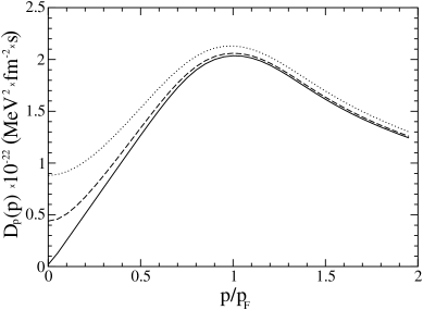
Figure 1: Dependence of the diffusion coefficient $D_{p}(p)$ on momentum $p$ in units of $p_{F}$, for temperatures $T=0.1$ MeV (solid line), $2\ \mathrm{MeV}$ (dashed line) and $4$ $\mathrm{MeV}$ (dotted line).

The results of calculations of the diffusion coefficient $D_{p}(p)$ accordingly to Eq. (15) with the Fermi distribution (16) are presented in Fig. 1. The calculations were performed for the different values of temperature $T$. As seen from Fig. 1, the momentum dependence of $D_{p}(p)$ has the clearly observed maximum at the Fermi momentum $p_{F}$ for different temperatures. With an increase of temperature the diffusion coefficient increases as $D_{p}(p=p_{F},T)\sim T^{2}$. The temperature dependence of the diffusion coefficient $D_{p}(p=p_{F},T)$ is shown in Fig. 2. As seen from Fig. 2, for a cold Fermi system the diffusion coefficient takes the non-zero value $D(p_{F},T=0)=2.1\cdot 10^{-22}$ $\mathrm{MeV}^{2}\mathrm{\cdot fm}^{-2}\mathrm{\cdot s}$ which is caused by the relaxation on the distorted Fermi-surface in Eq. (1) which exists at $T=0$ also. For high temperature regime where the Fermi statistic comes to Maxwell one, the diffusion coefficient $D(p_{F},T)$ behaves as a linear function of $T$ in agreement with the Einstein’s fluctuation-dissipation theorem.

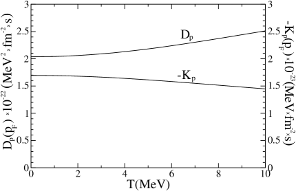
Figure 2: Dependence of the diffusion, $D_{p}$, and drift, $K_{p}$, coefficients taken at $p=p_{F}$ on the temperature $T$.

III.2 Drift term

Using Eq. (12) and $\varepsilon_{p}=p^{2}/2m$, one can write the drift coefficient $K_{p}(\mathbf{p})$ as

$$K_{p}(\mathbf{p})\frac{p_{\nu}}{m}=\nabla_{p,\nu}D_{p}(\mathbf{p})-\widehat{p}_{\nu}A(\mathbf{p}),$$ (17)

where

$$A(\mathbf{p})=\frac{1}{p}\int\frac{gd\mathbf{s}}{(2\pi\hbar)^{3}}\ p_{\nu}s_{\nu}\ W(\mathbf{p},\mathbf{s}).$$ (18)

For a spherically symmetric distribution $f(p)$ the drift coefficient $K_{p}(\mathbf{p})$ in Eq. (17) is reduced to the following form (see Appendix B)

$$K_{p}(p)=\frac{m}{p}\left(\frac{\partial D_{p}(p)}{\partial p}-A(p)\right),$$ (19)

where the first moment function $A(p)$ is given by Eq. (40) of Appendix B.

The presence of maximum of $D_{p}(p)$ at the Fermi momentum denotes that $\left.\partial D(p)/\partial p\right|_{p=p_{F}}=0$ and in agreement with Eq. (19) the drift coefficient $K_{p}(p_{F})$ is reduced as

$$K_{p}(p_{F})=-\frac{m}{p_{F}}A(p_{F}).$$ (20)

In Fig. 3 we show the dependence of the drift coefficient $K_{p}(p)$ on the momentum $p$ in units of Fermi momentum $p_{F}$. One can see that $K_{p}(p)$ has a minimum localized at $p<$ $p_{F}$ which slightly depends on the temperature. Note that for $p>p_{F}$ the temperature dependence of $K_{p}(p)$ is negligible.

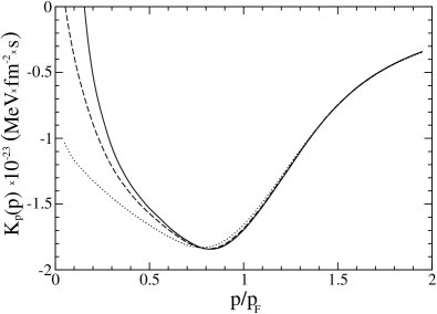
Figure 3: The same as in Fig. 1 but for the drift term $K_{p}(p)$.

The numerical estimates of the diffuse coefficient $D_{p}(p)$ and the drift term $K_{p}(p)$ near the Fermi momentum give $D_{p}(p_{F})\approx 10^{-22}$ $\mathrm{MeV}^{2}\mathrm{\cdot fm}^{-2}\cdot\mathrm{s}$ and $K_{p}(p_{F})\approx-10^{-23}$ $\mathrm{MeV\cdot fm}^{-2}\cdot\mathrm{s}$. Both obtained values of $D_{p}(p_{F})$ and $K_{p}(p_{F})$ agree with the phenomenological ones used earlier in Ref. wols82 .

IV Numerical results

Evaluating the transport coefficients $D_{p}(p)$ and $K_{p}(p)$ caused by the interparticle collisions on the distorted Fermi surface, we will restrict ourselves to a Fermi system which is homogeneous in $\mathbf{r}$ -space and omit the driving operator $\hat{L}$ in equation (10). Using the diffusion, $D_{p}(p)$, and drift, $K_{p}(p)$, coefficients from Eqs. (15) and (19), and solving the diffusion equation (10) with $\hat{L}=0$ one can evaluate the time evolution of the Wigner distribution function $f(p,t)$. We will also assume a spherical Fermi surface of radius $p_{F}$ which is derived by the condition for the particle number $A$ within a fixed volume $\mathcal{V}$

$$\int_{0}^{p_{F}}\frac{4\pi g\mathcal{V}}{(2\pi\hbar)^{3}}\ p^{2}dp=A.$$

The diffusion equation (10) must be augmented by the initial condition for $f(p,t)$.  We will consider the time evolution of the initial particle-hole ($1p1h$) excitation which is derived at $t=0$ as, see also Ref. wols82 ,

$$f_{\mathrm{in}}(p) = \left[1-\theta(p-p_{1}^{\prime})+\theta(p-p_{2}^{\prime})\right]\left[1-\theta(p-p_{F})\right]$$ (21)

$$+\left[1-\theta(p-p_{2})\right]\theta(p-p_{1})\theta(p-p_{F}).$$

The distribution $f_{\mathrm{in}}(p)$ of Eq. (21) means the particle located at $p_{1}<p<p_{2}$ and the hole excitation at $p_{1}^{\prime}<p<p_{2}^{\prime}$ for fixed $p_{1}>p_{F}$ and $p_{2}^{\prime}<p_{F}$, respectively. The intervals $\Delta p^{\prime}=p_{2}^{\prime}-p_{1}^{\prime}$ and $\Delta p=p_{2}-p_{1}$ are derived from the conditions

$$\int_{0}^{p_{F}}\frac{4\pi g\mathcal{V}dp}{(2\pi\hbar)^{3}}p^{2}f_{\mathrm{in}}(p,t=0) = A-1,$$

$$\int_{p_{F}}^{\infty}\frac{4\pi g\mathcal{V}dp}{(2\pi\hbar)^{3}}p^{2}f_{\mathrm{in}}(p,t=0) = 1.$$ (22)

In Fig. 4 we have plotted the time evolution of the Wigner distribution function $f(p,t)$ for the initial particle-hole excitation in the Fermi-system with $A=16$. We used the initial distribution $f_{\mathrm{in}}(p,t=0)$ given by Eq. (21) and assumed the initial excitation energy $E_{\mathrm{ex}}=30$ $\mathrm{MeV}$.

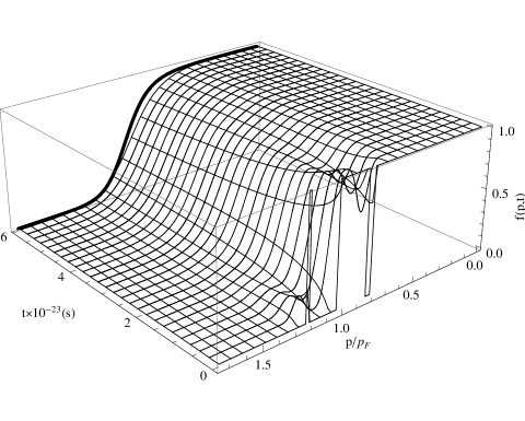
Figure 4: Time evolution of initial distribution function (21) in momentum space (in units of the Fermi momentum $p_{F}$) with $p_{1}^{\prime}/p_{F}\simeq 0.71$, $p_{2}^{\prime}/p_{F}\simeq 0.75$, $p_{1}/p_{F}\simeq 1.12$, $p_{2}/p_{F}\simeq 1.13$, which corresponds to the initial excitation energy $E_{\mathrm{ex}}=30$ MeV. The solid line is the equilibrium distribution $f_{\mathrm{eq}}(p)$.

One can see from Fig. 4 that the momentum distribution $f(p,t)$ evolves to the Fermi equilibrium limit $f_{\mathrm{eq}}(p)$ of Eq. (16) with temperature $T=\sqrt{E_{\mathrm{ex}}/a}$, where $a=(\pi^{2}/6)g(\epsilon_{F})$ is the level density parameter bomo1 and $g(\epsilon_{F})$ is the single-particle level density at the Fermi energy. The corresponding relaxation time $\tau_{r}$ for the diffusion process in Fig. 4 can be obtained considering the time evolution of the deviation $\delta f(p,t)=f(p,t)-f_{\mathrm{eq}}(p)$ of the distribution function $f(p,t)$ from its equilibrium limit $f_{\mathrm{eq}}(p)$. We introduce the mean square deviation

$$\Delta(t)=\int d\mathbf{p\ [}\delta f(p,t)\mathbf{]}^{2}-\left[\int d\mathbf{p\ }\delta f(p\mathbf{,}t\mathbf{)}\right]^{2}=\int d\mathbf{p\ [}\delta f(p,t)\mathbf{]}^{2}.$$ (23)

The time dependence of $\Delta(t)$ for the distribution function $f(p,t)$ from Fig. 4 is plotted in Fig. 5. The function $\Delta(t)$ can be fitted by the exponential dependence $\Delta(t)\sim$ $\exp(-t/\tau_{r})$ which is shown in Fig. 5 as the dashed line.

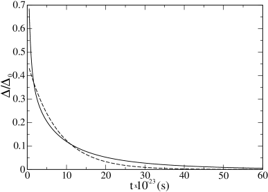
Figure 5: Dependence of the mean square deviation $\Delta(t)$ from Eq. (23) on the time (solid line). The dashed line is the mean square fit to the exponential function $\Delta(t)\sim\exp(-t/\tau_{r})$.

Both curves in Fig. 5 are normalized to the initial mean square deviation

$$\Delta_{0}=\int d\mathbf{p\ [}\delta f_{\mathrm{in}}(p)\mathbf{]}^{2},$$

where $\delta f_{\mathrm{in}}(p)=f_{\mathrm{in}}(p)-f_{\mathrm{eq}}(p)$. The corresponding relaxation time $\tau_{r}$ is estimated as $\tau_{r}\approx 8.3\cdot 10^{-23}\mathrm{s}$. The obtained value of $\tau_{r}$ agrees with a typical collisional relaxation time $\tau_{r,\mathrm{coll}}$ in a nucleus $\tau_{r,\mathrm{coll}}=10^{-23}\div 10^{-22}\mathrm{s}$ bert78 ; shko05 ; khol82 ; wegm74 .

We note also that considering the time evolution of the distribution function to the equilibrium (solid line in Fig. 4), we reach the regime where the further change of distribution function is negligible. That means that the collision integral in equation (10) should be zero in the case of equilibrium. To verify this fact we consider the time evolution of the collision integral (33). In Fig. 6 we show the ratio

$$R_{\mathrm{St}}(t)=\frac{\int d\mathbf{p\ [}\mathrm{St}\{f(t)\mathbf{\}]}^{2}}{\int d\mathbf{p\ [}\mathrm{St}\{f(t=0)\mathbf{\}]}^{2}},$$ (24)

which represents the time dependence of the mean square of collision integral $\mathrm{St}\{f(t)\}$ normalized to the initial value of $\mathrm{St}\{f(t=0)\}$.

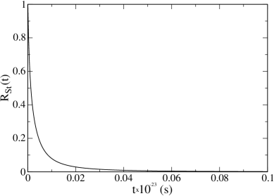
Figure 6: Time dependence of the ratio $R_{St}(t)$.

As seen from Fig. 6, the collision term $\mathrm{St}\{f(t)\}$ (33) approaches to zero with time as it should be in the equilibrium limit

V Conclusions

We have considered the kinetic approach with the collision integral for the Wigner distribution function using the diffusion approximation. We have demonstrated that the collisional Landau-Vlasov kinetic equation can be reduced to the form of the diffusion equation. We have established the expressions for both the diffusion coefficient $D_{p}(p)$ and the drift term $K_{p}(p)$ for the Fermi-systems where the relaxation processes occur on the distorted Fermi surface.

We have found out that the simplest isotropic assumption for the collision probability in the collision integral is insufficient for the correct description of the kinetic coefficients. The forward scattering should be ensured for the inter-particle interaction. For the description of the inter-particle interaction we have used the finite-range potential. Such kind of inter-particle interaction provides the necessary smallness of the momentum transfer and thereby the forward scattering of particles.

For the nuclear Fermi-liquid we have calculated dependencies of the diffuse coefficient $D_{p}(p)$ and the drift term $K_{p}(p)$ on the momentum $p$ and the temperature $T$. For the diffuse coefficient $D_{p}(p)$ the momentum dependence possesses the clearly observed maximum of order of $10^{-22}\ \mathrm{MeV}^{2}\mathrm{\cdot fm}^{-2}\mathrm{\cdot s}$ near the Fermi momentum for different temperatures. With an increase of temperature the value of the diffusion coefficient increases also. Excluding the small momentum values, the drift term $K_{p}(p)$ has negative sign and the minimum of order of $10^{-23}\ \mathrm{MeV\cdot fm}^{-2}\mathrm{\cdot s}$. Inside the Fermi sphere for $p<p_{F}$ the drift term $K_{p}(p)$ shows the strong dependence on the temperature. For $p>p_{F}$ the temperature dependence of $K_{p}(p)$ is practically negligible.

We have established the finite value of the diffusion coefficient in a cold Fermi system with $D(p_{F},T=0)=2.1\cdot 10^{-22}$ $\mathrm{MeV}^{2}\cdot\mathrm{fm}^{-2}\cdot\mathrm{s}$ which is caused by the relaxation on the distorted Fermi-surface at $T=0$. The diffusion process was investigated numerically assuming the initial non-equilibrium $1p1h$-excitation for a finite Fermi-system with number of particles $A=16$. It was shown that the $1p1h$-excitation relaxes to the equilibrium Fermi distribution. The numerical estimate for the relaxation time $\tau_{r}$ gives $\tau_{r}\approx 8.3\cdot 10^{-23}s$ which is close to the corresponding estimates in a nuclear Fermi-liquid obtained within the kinetic theory.

Appendix A Moment representation for the collision integral.

Applying the expansions of $W(\mathbf{p}_{1},\mathbf{p}_{3})$ and $\widetilde{W}(\mathbf{p}_{1},\mathbf{p}_{3})$ over small $\mathbf{s}=\mathbf{p}_{3}-\mathbf{p}_{1}$ (see Eqs. (7) and (8)), the collision integral (3) can be written as

$$\mathrm{St}\{f\} \approx \int\frac{gd\mathbf{s}}{(2\pi\hbar)^{3}}\left[\left(W(\mathbf{p}_{1},\mathbf{s})-\widetilde{W}(\mathbf{p}_{1},\mathbf{s})\right)\tilde{f}(\mathbf{p}_{1})f(\mathbf{p}_{1})\right.$$ (25)

$$+ s_{\nu}\left\{\left(W(\mathbf{p}_{1},\mathbf{s})\tilde{f}(\mathbf{p}_{1})+\widetilde{W}(\mathbf{p}_{1},\mathbf{s})f(\mathbf{p}_{1})\right)\nabla_{p_{1},\nu}f(\mathbf{p}_{1})\right.$$

$$+ \left.\frac{1}{2}\tilde{f}(\mathbf{p}_{1})f(\mathbf{p}_{1})\nabla_{p_{1},\nu}\left(W(\mathbf{p}_{1},\mathbf{s})-\widetilde{W}(\mathbf{p}_{1},\mathbf{s})\right)\right\}$$

$$+ \frac{1}{2}s_{\nu}s_{\mu}\left\{W(\mathbf{p}_{1},\mathbf{s})\tilde{f}(\mathbf{p}_{1})\nabla_{p_{1},\nu}\nabla_{p_{1},\mu}f(\mathbf{p}_{1})\right.$$

$$+ \left.\left(\tilde{f}(\mathbf{p}_{1})\nabla_{p_{1},\nu}W(\mathbf{p}_{1},\mathbf{s})+f(\mathbf{p}_{1})\nabla_{p_{1},\nu}\widetilde{W}(\mathbf{p}_{1},\mathbf{s})\right)\nabla_{p_{1},\mu}f(\mathbf{p}_{1})\right.$$

$$+ f(\mathbf{p}_{1})\left(\widetilde{W}(\mathbf{p}_{1},\mathbf{s})\nabla_{p_{1},\nu}\nabla_{p_{1},\mu}f(\mathbf{p}_{1})\right.$$

$$+ \left.\left.\left.\frac{1}{4}\tilde{f}(\mathbf{p}_{1})\nabla_{p_{1},\nu}\nabla_{p_{1},\mu}\left(W(\mathbf{p}_{1},\mathbf{s})-\widetilde{W}(\mathbf{p}_{1},\mathbf{s})\right)\right)\right\}\right].$$

Using then Eqs. (4),  (5) and (9), we obtain

$$W(\mathbf{P},\mathbf{s}) \simeq \frac{2g}{m^{2}}\frac{d\sigma}{d\Omega}(\mathbf{s}^{2})\int d\mathbf{p}_{2}d\mathbf{p}_{4}\tilde{f}(\mathbf{p}_{2})f(\mathbf{p}_{4})\delta\left(\mathbf{p}_{2}-\mathbf{p}_{4}-\mathbf{s}\right)$$ (26)

$$\times \delta\left(\varepsilon_{2}-\varepsilon_{4}-\frac{\mathbf{P\cdot}\mathbf{s}}{m}\right)$$

and

$$\widetilde{W}(\mathbf{P},\mathbf{s}) \simeq \frac{2g}{m^{2}}\frac{d\sigma}{d\Omega}(\mathbf{s}^{2})\int d\mathbf{p}_{2}d\mathbf{p}_{4}\ f(\mathbf{p}_{2})\tilde{f}(\mathbf{p}_{4})\delta\left(\mathbf{p}_{2}-\mathbf{p}_{4}-\mathbf{s}\right)$$ (27)

$$\times \delta\left(\varepsilon_{2}-\varepsilon_{4}-\frac{\mathbf{P\cdot}\mathbf{s}}{m}\right).$$

The collision integral of Eq. (25) is transformed to the following form

$$\mathrm{St}\{f\} = \int\frac{gd\mathbf{s}}{(2\pi\hbar)^{3}}\ s_{\nu}\left\{W(\mathbf{p}_{1},\mathbf{s})\left(\tilde{f}(\mathbf{p}_{1})-f(\mathbf{p}_{1})\right)\nabla_{p_{1},\nu}f(\mathbf{p}_{1})+\tilde{f}(\mathbf{p}_{1})f(\mathbf{p}_{1})\right.$$ (28)

$$\times \left.\nabla_{p_{1},\nu}W(\mathbf{p}_{1},\mathbf{s})\right\}+\frac{1}{2}\int\frac{gd\mathbf{s}}{(2\pi\hbar)^{3}}\ s_{\nu}s_{\mu}\left\{W(\mathbf{p}_{1},\mathbf{s})\tilde{f}(\mathbf{p}_{1})\nabla_{p_{1},\nu}\nabla_{p_{1},\mu}f(\mathbf{p}_{1})\right.$$

$$+ \nabla_{p_{1},\nu}\left(W(\mathbf{p}_{1},\mathbf{s})\right)\nabla_{p_{1},\mu}f(\mathbf{p}_{1})+\left.W(\mathbf{p}_{1},\mathbf{s})f(\mathbf{p}_{1})\nabla_{p_{1},\nu}\nabla_{p_{1},\mu}f(\mathbf{p}_{1})\right\}.$$

Introducing the two first moments $A_{\nu}(\mathbf{p}_{1})$ and $B_{\nu\mu}(\mathbf{p}_{1})$ of scattering probability $W(\mathbf{p}_{1},\mathbf{s})$ as

$$A_{\nu}(\mathbf{p}_{1})=\int\frac{gd\mathbf{s}}{(2\pi\hbar)^{3}}\ s_{\nu}\ W(\mathbf{p}_{1},\mathbf{s}),\quad B_{\nu\mu}(\mathbf{p}_{1})=\frac{1}{2}\int\frac{gd\mathbf{s}}{(2\pi\hbar)^{3}}\ s_{\nu}s_{\mu}\ W(\mathbf{p}_{1},\mathbf{s}),$$ (29)

the collision integral (28) is reduced as

$$\mathrm{St}\{f\}=\nabla_{p_{1},\nu}\left[A_{\nu}(\mathbf{p}_{1})f(\mathbf{p}_{1})\tilde{f}(\mathbf{p}_{1})+B_{\nu\mu}(\mathbf{p}_{1})\nabla_{p_{1},\mu}f(\mathbf{p}_{1})\right].$$ (30)

Using the relations

$$B_{\nu\mu}(\mathbf{p}_{1})\nabla_{p_{1},\mu}f(\mathbf{p}_{1})$$ (31)

$$= \nabla_{p_{1},\mu}\left(B_{\nu\mu}(\mathbf{p}_{1})\tilde{f}(\mathbf{p}_{1})f(\mathbf{p}_{1})\right)-\tilde{f}(\mathbf{p}_{1})f(\mathbf{p}_{1})\nabla_{p_{1},\mu}B_{\nu\mu}(\mathbf{p}_{1})+B_{\nu\mu}(\mathbf{p}_{1})\nabla_{p_{1},\mu}f^{2}(\mathbf{p}_{1})$$

$$= \nabla_{p_{1},\mu}\left(B_{\nu\mu}(\mathbf{p}_{1})f(\mathbf{p}_{1})\right)-f^{2}(\mathbf{p}_{1})\nabla_{p_{1},\mu}B_{\nu\mu}(\mathbf{p}_{1})-\tilde{f}(\mathbf{p}_{1})f(\mathbf{p}_{1})\nabla_{p_{1},\mu}B_{\nu\mu}(\mathbf{p}_{1}),$$

we rewrite the collision integral (30) as

$$\mathrm{St}\{f\} = -\ \nabla_{p_{1},\nu}\left[\left\{\nabla_{p_{1},\mu}B_{\nu\mu}(\mathbf{p}_{1})-A_{\nu}(\mathbf{p}_{1})\right\}f(\mathbf{p}_{1})\tilde{f}(\mathbf{p}_{1})+f^{2}(\mathbf{p}_{1})\nabla_{p_{1},\mu}B_{\nu\mu}(\mathbf{p}_{1})\right]$$ (32)

$$+ \nabla_{p_{1},\nu}\nabla_{p_{1},\mu}(f(\mathbf{p}_{1})B_{\nu\mu}(\mathbf{p}_{1})).$$

Finally, we obtain

$$\mathrm{St}\{f\} = -\ \nabla_{p_{1},\nu}\left[K_{p}(\mathbf{p}_{1})(\nabla_{p_{1},\nu}\varepsilon_{p_{1}})f(\mathbf{p}_{1})\tilde{f}(\mathbf{p}_{1})+f^{2}(\mathbf{p}_{1})\nabla_{p_{1},\nu}D_{p}(\mathbf{p}_{1})\right]$$ (33)

$$+ \nabla_{p_{1},\nu}^{2}\,\left[f(\mathbf{p}_{1})\,D_{p}(\mathbf{p}_{1})\right].$$

Appendix B Diffuse and drift terms

Integrating in Eq. (14) over $\mathbf{s}$, one obtains

$$D_{p}(\mathbf{p}_{1}) \approx \frac{g^{2}r_{0}^{6}v_{0}^{2}}{48\pi^{2}\hbar^{7}}\int d\mathbf{p}_{2}d\mathbf{p}_{4}\ (\mathbf{p}_{2}-\mathbf{p}_{4})^{2}\exp\left(-4(\mathbf{p}_{2}-\mathbf{p}_{4})^{2}r_{0}^{2}/\hbar^{2}\right)\tilde{f}(\mathbf{p}_{2})f(\mathbf{p}_{4})$$ (34)

$$\times \delta\left(\varepsilon_{2}-\varepsilon_{4}-\frac{\mathbf{p}_{1}}{m}(\mathbf{p}_{2}-\mathbf{p}_{4})\right).$$

The argument of the delta function in Eq. (34) can be written as

$$\varepsilon_{2}-\varepsilon_{4}-\frac{\mathbf{p}_{1}}{m}(\mathbf{p}_{2}-\mathbf{p}_{4})=\frac{1}{2m}\left((\mathbf{p}_{2}-\mathbf{p}_{1})^{2}-(\mathbf{p}_{4}-\mathbf{p}_{1})^{2}\right),$$

where $\varepsilon_{j}=\mathbf{p}_{j}^{2}/2m$. We will introduce the new variables $\mathbf{p}_{2}-\mathbf{p}_{1}=\mathbf{q}$ and $\mathbf{p}_{4}-\mathbf{p}_{1}=\mathbf{k}$ which allows one to rewrite Eq. (34) in the following form

$$D_{p}(\mathbf{p}_{1}) \approx \frac{g^{2}mr_{0}^{6}v_{0}^{2}}{24\pi^{2}\hbar^{7}}\int d\mathbf{q}\ d\mathbf{k}\ (\mathbf{q}-\mathbf{k})^{2}\exp\left(-4(\mathbf{q}-\mathbf{k})^{2}r_{0}^{2}/\hbar^{2}\right)\tilde{f}(\mathbf{q}+\mathbf{p}_{1})f(\mathbf{k}+\mathbf{p}_{1})$$ (35)

$$\times \delta\left(\mathbf{q}^{2}-\mathbf{k}^{2}\right).$$

Using the spherically symmetric distribution function $f(\mathbf{p})$ and the relation

$$\delta\left(x^{2}-a^{2}\right)=\frac{\delta(x-a)+\delta(x+a)}{2|a|},$$

we will rewrite Eq. (35) as

$$D_{p}(\mathbf{p}_{1}) \approx \frac{g^{2}mr_{0}^{6}v_{0}^{2}}{48\pi^{2}\hbar^{7}}\int_{0}^{\infty}q^{2}dq\ \int d\Omega_{q}\int_{0}^{\infty}kdk\ \int d\Omega_{k}\left(q^{2}+k^{2}-2qk\cos\widehat{\mathbf{q}\mathbf{k}}\right)$$ (36)

$$\times \exp\left(-4(q^{2}+k^{2}-2qk\cos\widehat{\mathbf{q}\mathbf{k}})r_{0}^{2}/\hbar^{2}\right)\left\{\delta(q-k)+\delta(q+k)\right\}$$

$$\times \tilde{f}\left(\sqrt{q^{2}+p_{1}^{2}+2qp_{1}\cos\widehat{\mathbf{q}\mathbf{p}_{1}}}\right)f\left(\sqrt{k^{2}+p_{1}^{2}+2kp_{1}\cos\widehat{\mathbf{k}\mathbf{p}_{1}}}\right).$$

Integrating in Eq. (36) over $q$, we obtain

$$D_{p}(\mathbf{p}_{1}) \approx \frac{g^{2}mr_{0}^{6}v_{0}^{2}}{24\pi^{2}\hbar^{7}}\int_{0}^{\infty}dk\ k^{5}\int d\Omega_{k}\int d\Omega_{q}\ \left(1-\cos\widehat{\mathbf{q}\mathbf{k}}\right)$$ (37)

$$\times \exp\left(-8k^{2}r_{0}^{2}(1-\cos\widehat{\mathbf{q}\mathbf{k}})/\hbar^{2}\right)\tilde{f}\left(\sqrt{k^{2}+p_{1}^{2}+2kp_{1}\cos\widehat{\mathbf{q\cdot}\mathbf{p}_{1}}}\right)$$

$$\times f\left(\sqrt{k^{2}+p_{1}^{2}+2kp_{1}\cos\widehat{\mathbf{k\cdot}\mathbf{p}_{1}}}\right).$$

Using the addition theorem for spherical harmonics, we can write in an arbitrary spherical coordinate system

$$\cos\widehat{\mathbf{q\cdot}\mathbf{k}} = \cos\theta_{q}\cos\theta_{k}+\sin\theta_{q}\sin\theta_{k}\cos(\phi_{q}+\phi_{k}),$$

$$\cos\widehat{\mathbf{q\cdot}\mathbf{p}_{1}} = \cos\theta_{q}\cos\theta_{p_{1}}+\sin\theta_{q}\sin\theta_{p_{1}}\cos(\phi_{q}+\phi_{p_{1}}),$$

$$\cos\widehat{\mathbf{k\cdot}\mathbf{p}_{1}} = \cos\theta_{k}\cos\theta_{p_{1}}+\sin\theta_{k}\sin\theta_{p_{1}}\cos(\phi_{k}+\phi_{p_{1}}).$$

Taking into account the spherically symmetry of the distribution functions $f(\mathbf{p}_{j})=f(p_{j})$ and using

$$\cos\widehat{\mathbf{q\cdot}\mathbf{p}_{1}}=\cos\theta_{q},\qquad\cos\widehat{\mathbf{k\cdot}\mathbf{p}_{1}}=\cos\theta_{k},$$

we obtain

$$D_{p}(p_{1}) \approx \frac{g^{2}mr_{0}^{6}v_{0}^{2}}{24\pi^{2}\hbar^{7}}\int_{0}^{\infty}dk\ k^{5}\int d\Omega_{k}\int d\Omega_{q}\ \left(1-\cos\widehat{\mathbf{q}\mathbf{k}}\right)$$ (38)

$$\times \exp\left(-8k^{2}r_{0}^{2}(1-\cos\widehat{\mathbf{q}\mathbf{k}})/\hbar^{2}\right)\tilde{f}\left(\sqrt{k^{2}+p_{1}^{2}+2kp_{1}\cos\theta_{q}}\right)$$

$$\times f\left(\sqrt{k^{2}+p_{1}^{2}+2kp_{1}\cos\theta_{k}}\right).$$

We will also introduce the following notations

$$j(\alpha)=\int_{0}^{2\pi}d\phi_{q}\int_{0}^{2\pi}d\phi_{k}\ \exp\left(\alpha(\phi_{q}+\phi_{k})\right),$$

$$\widetilde{j}(\alpha)=\int_{0}^{2\pi}d\phi_{q}\int_{0}^{2\pi}d\phi_{k}\ \cos(\phi_{q}+\phi_{k})\exp\left(\alpha(\phi_{q}+\phi_{k})\right),$$

which are attributed as functions of the argument $\alpha$. Using $j(\alpha)$ and $\widetilde{j}(\alpha)$, one can write the angular integrals in Eq. (38) as

$$\int_{0}^{2\pi}d\phi_{q}\int_{0}^{2\pi}d\phi_{k}\ \left(1-\cos\widehat{\mathbf{q}\mathbf{k}}\right)\exp\left(-8k^{2}r_{0}^{2}(1-\cos\widehat{\mathbf{q}\mathbf{k}})/\hbar^{2}\right)$$

$$= \exp\left(-8k^{2}r_{0}^{2}(1-\cos\theta_{q}\cos\theta_{k})/\hbar^{2}\right)$$

$$\times \left\{(1-\cos\theta_{q}\cos\theta_{k})j(8k^{2}r_{0}^{2}\sin\theta_{q}\sin\theta_{k}/\hbar^{2})-\sin\theta_{q}\sin\theta_{k}\ \widetilde{j}(8k^{2}r_{0}^{2}\sin\theta_{q}\sin\theta_{k}/\hbar^{2})\right\}$$

Finally, we obtain the diffuse coefficient $D_{p}(p)$ in the form given by Eq. (15).

The drift coefficient $K_{p}(\mathbf{p})$ of Eq. (12) can be reduced similarly to above described procedure. Using derivation of Eq. (18), we will reduce $A(\mathbf{p}_{1})$ to the following form

$$A(\mathbf{p}_{1}) \approx \frac{g^{2}mr_{0}^{6}v_{0}^{2}}{4\pi^{2}\hbar^{7}p_{1}}\int d\mathbf{q}\ d\mathbf{k}\ \mathbf{p}_{1}(\mathbf{q}-\mathbf{k})\exp\left(-4(\mathbf{q}-\mathbf{k})^{2}r_{0}^{2}/\hbar^{2}\right)\tilde{f}(\mathbf{q}+\mathbf{p}_{1})f(\mathbf{k}+\mathbf{p}_{1})$$

$$\times \delta\left(\mathbf{q}^{2}-\mathbf{k}^{2}\right),$$

or

$$A(p_{1}) \approx \frac{g^{2}mr_{0}^{6}v_{0}^{2}}{8\pi^{2}\hbar^{7}}\int_{0}^{\infty}dk\ k^{4}\int d\Omega_{k}\int d\Omega_{q}\ \left(\cos\theta_{q}-\cos\theta_{k}\right)$$ (39)

$$\times \exp\left(-8k^{2}r_{0}^{2}(1-\cos\widehat{\mathbf{q}\mathbf{k}})/\hbar^{2}\right)\tilde{f}\left(\sqrt{k^{2}+p_{1}^{2}+2kp_{1}\cos\theta_{q}}\right)$$

$$\times f\left(\sqrt{k^{2}+p_{1}^{2}+2kp_{1}\cos\theta_{k}}\right).$$

Finally, we obtain

$$A(p) \approx \frac{g^{2}mr_{0}^{6}v_{0}^{2}}{8\pi^{2}\hbar^{7}}\int_{0}^{\infty}dk\ k^{4}\int_{-1}^{1}dx\int_{-1}^{1}dy\ (x-y)$$ (40)

$$\times \exp\left(-8k^{2}r_{0}^{2}(1-xy)/\hbar^{2}\right)j\left(8k^{2}r_{0}^{2}\sqrt{1-x^{2}}\sqrt{1-y^{2}}/\hbar^{2}\right)$$

$$\times \tilde{f}\left(\sqrt{k^{2}+p^{2}+2kp_{1}x}\right)f\left(\sqrt{k^{2}+p^{2}+2kpy}\right).$$

References

(1) V.M. Kolomietz and S. Shlomo, Phys. Rep. 390, 133
(2004).
(2) G. Bertsch, Z. Phys. A289, 103 (1978).
(3) V.M. Kolomietz, V.A. Plujko and S. Shlomo, Phys. Rev. C
52, 2480 (1995).
(4) A.G. Magner, V.M. Kolomietz, H. Hofmann and S.Shlomo, Phys.
Rev. C51, 2457 (1995).
(5) D. Kiderlen, V.M. Kolomietz and S. Shlomo, Nucl. Phys.
A608, 32 (1996).
(6) V.M. Kolomietz, V.A. Plujko and S.Shlomo, Phys. Rev. C
54, 3014 (1996).
(7) M. Di Toro, V.M. Kolomietz and A.B. Larionov, Phys. Rev.
C59, 3099 (1999).