Anisotropic models for compact stars

Abstract

In the present paper we obtain an anisotropic analogue of Durgapal-Fuloria Durgapal1985 perfect fluid solution. The methodology consists of contraction of anisotropic factor $\Delta$ by the help of both metric potentials $e^{\nu}$ and $e^{\lambda}$. Here we consider $e^{\lambda}$ same as Durgapal-Fuloria Durgapal1985 whereas $e^{\nu}$ is that given by Lake Lake2003 . The field equations are solved by the change of dependent variable method. The solutions set mathematically thus obtained are compared with the physical properties of some of the compact stars, strange star as well as white dwarf. It is observed that all the expected physical features are available related to stellar fluid distribution which clearly indicate validity of the model.

1 Introduction

Few decades ago a new analytic relativistic model was obtained by Durgapal and Fuloria Durgapal1985 for superdense stars in the framework of Einstein’s General Theory of Relativity. They showed that the model in connection to neutron star stands all the tests of physical reality with the maximum mass $4.17~{}M_{\odot}$ and the surface redshift $0.63$. Very recently Gupta and Maurya Gupta2011 presented a class of charged analogues of superdense star model due to Durgapal and Fuloria Durgapal1985 under the Einstein-Maxwell spacetimes. The members of this class have been shown to satisfy various physical conditions and exhibit features (i) with the maximum mass $3.2860~{}M_{\odot}$ and the radius $18.3990$ km for a particular interval of the parameter $1<K\leq 1.7300$, and (ii) with the maximum mass $1.9672~{}M_{\odot}$ and the radius $15.9755$ km for another interval of the parameter $1<K\leq 1.1021$. Later on a family of well behaved charged analogues of Durgapal and Fuloria Durgapal1985 perfect fluid exact solution was also obtained by Murad and Fatema Murad2014 where they have studied the Crab pulsar with radius $13.21$ km.

In a similar way we have considered a generalization of Durgapal and Fuloria Durgapal1985 with anisotropic fluid sphere such that $p_{r}\neq p_{t}$, where $p_{r}$ and $p_{t}$ respectively are radial and tangential pressures of fluid distribution. The present work is a sequel of the paper Maurya2015 where we have developed a general algorithm in the form of metric potential $\nu$ for all spherically symmetric charged anisotropic solutions in connection to compact stars. However, in the present study without considering any anisotropic function we can develop algorithm by the help of metric potentials only and here lies the beauty of the investigation. Another point we would like to add here that till now, as far as our knowledge is concerned, no alternative anisotropic analogue of Duragapal-Fuloria Durgapal1985 solution is available in the literature.

In connection to anisotropy we note that it was Ruderman Ruderman1972 who argued that the nuclear matter may have anisotropic features at least in certain very high density ranges ($>~{}10^{15}~{}gm/cm^{3}$) and thus the nuclear interaction can be treated under relativistic background. Later on Bowers and Liang Bowers1974 specifically investigated the non-negligible effects of anisotropy on maximum equilibrium mass and surface redshift. In this regard several recently performed anisotropic compact star models may be consulted for further reference  Mak2002 ; Mak2003a ; Usov2004 ; Varela2010 ; Rahaman2010a ; Rahaman2011 ; Rahaman2012a ; Kalam2012 ; Bhar2015 . We also note some special works with anisotropic aspect in the physical system like Globular Clusters, Galactic Bulges and Dark Halos in the Refs. Nguyen2013a ; Nguyen2013b .

As a special feature of anisotropy we note that for small radial increase the anisotropic parameter increases. However, after reaching a maximum in the interior of the star it becomes a decreasing function of the radial distance as shown by Mak and Harko Mak2004a ; Mak2004b . Obviously at the centre of the fluid sphere the anisotropy is expected to vanish.

We would like to mention that algorithm for perfect fluid and anisotropic uncharged fluid is already available in the literature Lake2003 ; Lake2004 ; Herrera2008 . As for example, we note that in his work Lake Lake2003 ; Lake2004 has considered an algorithm based on the choice of a single monotone function which generates all regular static spherically symmetric perfect as well as anisotropic fluid solutions under the Einstein spacetimes. It is also observed that Herrera et al. Herrera2008 have extended the algorithm to the case of locally anisotropic fluids. Thus we opt for an algorithm to a more general case with anisotropic fluid distribution. However, in this context it is to note that in the Ref. Maurya2015 we developed an algorithm in the Einstein-Maxwell spacetimes.

The outline of the present paper can be put as follows: in Sec. 2 the Einstein field equations for anisotropic stellar source are given whereas the general solutions are shown in Sec. 3 along with the necessary matching condition. In Sec. 4 we represent interesting features of the physical parameters which include density, pressure, stability, charge, anisotropy and redshift. As a special study we provide several data sheets in connection to compact stars. Sec. 5 is used as a platform for some discussions and conclusions.

2 The Einstein field equations

In this work we intend to study a static and spherically symmetric matter distribution whose interior metric is given in Schwarzschild coordinates, $x^{i}=(r,\theta,\phi,t)$ Tolman1939 ; Oppenheimer1939

$$ds^{2}=-e^{\lambda(r)}dr^{2}-r^{2}(d\theta^{2}+sin^{2}\theta d\phi^{2})+e^{\nu(r)}dt^{2}.$$ (1)

The functions $\nu$ and $\lambda$ satisfy the Einstein field equations,

$$\kappa{T^{i}}_{j}={R^{i}}_{j}-\frac{1}{2}R{g^{i}}_{j}.$$ (2)

where $\kappa=8\pi$ is the Einstein constant with $G=1=c$ in relativistic geometrized unit, $G$ and $c$ respectively being the Newtonian gravitational constant and velocity of photon in vacua.

The matter within the star is assumed to be locally anisotropic fluid in nature and consequently ${T^{i}}_{j}$ is the energy-momentum tensor of fluid distribution defined by

$${T^{i}}_{j}=[(\rho+p_{r})v^{i}v_{j}-p_{t}{\delta^{i}}_{j}+(p_{r}-p_{t})\theta^{i}\theta_{j}],$$ (3)

where $v^{i}$ is the four-velocity as $e^{\lambda(r)/2}v^{i}={\delta^{i}}_{4}$, $\theta^{i}$ is the unit space like vector in the direction of radial vector, $\theta^{i}=e^{\lambda(r)/2}{\delta^{i}}_{1}$ is the energy density, $p_{r}$ is the pressure in direction of $\theta^{i}$ (normal pressure) and $p_{t}$ is the pressure orthogonal to $\theta_{i}$ (transverse or tangential pressure).

For the spherically symmetric metric (1), the Einstein field equations may be expressed as the following system of ordinary differential equations Dionysiou1982

$$-\kappa{T^{1}}_{1}=\frac{{\nu}^{\prime}}{r}e^{-\lambda}-\frac{(1-e^{-\lambda})}{r^{2}}=\kappa p_{r},$$ (4)

$$-\kappa{T^{2}}_{2}=-\kappa{T^{3}}_{3}=\left[\frac{{\nu}^{\prime\prime}}{2}-\frac{{\lambda}^{\prime}{\nu}^{\prime}}{4}+\frac{{{\nu}^{\prime}}^{2}}{4}+\frac{{\nu}^{\prime}-{\lambda}^{\prime}}{2r}\right]e^{-\lambda}=\kappa p_{t},$$ (5)

$$\kappa{T^{4}}_{4}=\frac{{\lambda}^{\prime}}{r}e^{-\lambda}+\frac{(1-e^{-\lambda})}{r^{2}}=\kappa\rho,$$ (6)

where the prime denotes differential with respect to radial coordinate $r$.

The pressure anisotropy condition for the system can be provided as

$$\Delta=\kappa\left(p_{t}-p_{r}\right)=\left[\frac{{\nu}^{\prime\prime}}{2}-\frac{{\lambda}^{\prime}{\nu}^{\prime}}{4}+\frac{{{\nu}^{\prime}}^{2}}{4}+\frac{{\nu}^{\prime}-{\lambda}^{\prime}}{2r}\right]e^{-\lambda}-\frac{{\nu}^{\prime}}{r}e^{-\lambda}+\frac{(1-e^{-\lambda})}{r^{2}}.$$ (7)

Now let us consider the metric potentials Durgapal1985 in the following forms:

$$e^{-\lambda}=\frac{7-10Cr^{2}-C^{2}r^{4}}{7+14Cr^{2}+7C^{2}r^{4}},$$ (8)

$$\nu=2\ln\psi,$$ (9)

where $C$ is a positive constant and $\psi$ is a function which depends on radial coordinate $r$. The nature of plots for these quantities are shown in Fig. 1.

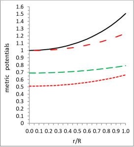
Figure 1: Variation of the metric potentials with radial coordinate $r/R$ are shown in the above figure. Here the legends are as follows: (i) $e^{\nu}$ is plotted with dotted line for Her X-1 and short-dashed line for white dwarf, (ii) $e^{\lambda}$ is plotted with continuous line for Her X-1 and long-dashed line for white dwarf

The above Eq. (7) together with Eqs. (8) and (9) becomes

$$\Delta=\left[\frac{7-10Cr^{2}-C^{2}r^{4}}{7(1+Cr^{2})^{2}}\right]\frac{{\psi}^{\prime\prime}}{\psi}+\left[\frac{C^{3}r^{6}+19C^{2}r^{4}-21Cr^{2}-7}{7r(1+Cr^{2})^{3}}\right]\frac{{\psi}^{\prime}}{\psi}+\left[\frac{8C^{2}r^{2}(Cr^{2}+5)}{7(1+C{r}^{2})^{3}}\right].$$ (10)

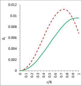
Figure 2: Variation of the anisotropy factor with radial coordinate $r/R$ are shown in figure. Here the legends are as follows: (i) $\Delta$ is plotted with short-dashed line for Her X-1, (ii) $\Delta$ is plotted with continuous line for white dwarf

3 The solutions for the model

Here our initial aim is to find out the pressure anisotropic function $\Delta$, which is zero at the centre and monotonic increasing for suitable choices of $\psi$. However, Lake Lake2003 imposes condition that $\psi$ should be regular and monotonic increasing function of radial coordinate $r$.

Let us therefore take the form of $\psi$ as follows:

$$\psi=(1-\alpha+Cr^{2})^{2},$$ (11)

where $\alpha>0$.

Substituting the value of $\psi$ from Eq. (11) in Eq. (10), we get

$$\Delta=-{\frac{8}{7}}\,{\frac{\alpha\,{C}^{2}{r}^{2}[2\,{C}^{2}{r}^{4}+\left(16-\alpha\right)C{r}^{2}-5\,\alpha-2]}{\left(1+C{r}^{2}\right)^{3}\left(1-\alpha+C{r}^{2}\right)^{2}}}.$$ (12)

For $\alpha>0$ and $0<Cr^{2}<\frac{\sqrt{{\alpha}^{2}+8\alpha+272}-(16-K)}{4}$, the pressure anisotropy is finite as well as positive everywhere as can be seen in Fig. 2.

By inserting the above value of $\Delta$ in the Eq. (12), we get

$$\psi^{\prime\prime}+\left[\frac{C^{3}r^{6}+19C^{2}r^{4}-21Cr^{2}-7}{r(1+Cr^{2})(7-10Cr^{2}-C^{2}r^{4})}\right]\psi^{\prime}$$

$$+\frac{1}{7-10Cr^{2}-C^{2}r^{4}}\left[\frac{8C^{2}r^{2}(Cr^{2}+5)}{(1+Cr^{2})}+\frac{8\alpha C^{2}r^{2}[2C^{2}r^{4}+(16-\alpha)Cr^{2}-(5\alpha+2)]}{(1+Cr^{2})(1-\alpha+Cr^{2})^{2}}\right]\psi=0.$$ (13)

Now our next task is to obtain the most general solution of the differential Eq. (13). Here we shall use the change of dependent variable method. We consider the differential equation of the form

$$y^{\prime\prime}+p(r)y^{\prime}+q(r)y=0.$$ (14)

Let $y=y_{1}$ be the particular solution of the differential Eq. (14). Then $y=y_{1}U$ will be complete solution of the differential Eq. (14), where

$$U=a_{1}+b_{1}\int\exp\left[-\int(p(r)+\frac{2y^{\prime}}{y_{1}})dr\right]dr,$$

where $a_{1}$ and $b_{1}$ are arbitrary constants.

Again let us consider here that $\psi=(1-\alpha+Cr^{2})^{2}=\psi_{\alpha r}$ is a particular solution of Eq. (13). So, the most general solution of the differential Eq. (13) can be given by

$$\psi=(1-\alpha+Cr^{2})^{2}\left[\tilde{B}+\tilde{A}\int\exp\left\{-\int\left(\frac{C^{3}r^{6}+19C^{2}r^{4}-21Cr^{2}-7}{r(1+Cr^{2})(7-10Cr^{2}-C^{2}r^{4})}+\frac{8Cr^{2}}{r(1-\alpha+Cr^{2})}\right)dr\right\}dr\right],$$ (15)

where $\tilde{A}$ and $\tilde{B}$ are arbitrary constants.

After integrating it, we get

$$\psi=\psi_{\alpha r}\left[B-A\left\{\frac{\{\psi_{\alpha 1}+\psi_{\alpha 2}(1-\alpha+Cr^{2})+\psi_{\alpha 3}\psi_{\alpha r}\}\sqrt{(\psi_{\alpha 5}-2(4+\alpha)(1-\alpha+Cr^{2})-\psi_{\alpha r})}}{(1-\alpha+Cr^{2})^{3}}+W(r)\right\}\right],$$ (16)

where

$$\psi_{\alpha r}=(1-\alpha+Cr^{2})^{2},$$ (17)

$$W(r)=\frac{\psi_{\alpha 4}}{\sqrt{\psi_{\alpha 5}}}\log\left[\frac{\psi_{\alpha 5}-(4+\alpha)(1-\alpha+Cr^{2})+\sqrt{\psi_{\alpha 5}}\sqrt{(\psi_{\alpha 5}-2(4+\alpha)(1-\alpha+Cr^{2})-\psi_{\alpha r})}}{(1-\alpha+Cr^{2})\psi_{\alpha 5}}\right],$$ (18)

and $A$ and $B$ are arbitrary constants with

$\psi_{\alpha 1}=\frac{\alpha}{3(16-8\alpha-\alpha^{2})}$,

$\psi_{\alpha 2}=\frac{24-2\alpha+\alpha^{2}}{3(16-8\alpha-\alpha^{2})^{2}}$,

$\psi_{\alpha 3}=\frac{288+80\alpha-10\alpha^{2}+\alpha^{3}}{3(16-8\alpha-\alpha^{2})^{3}}$,

$\psi_{\alpha 4}=\frac{1536-384\alpha+48\alpha^{2}-2\alpha^{3}}{3(16-8\alpha-\alpha^{2})^{3}}$,

$\psi_{\alpha 5}=(16-8\alpha-\alpha^{2})$.

Using Eqs. (8), (12) and (16) the expressions for energy-density and pressure read as

$$\frac{\kappa\rho}{C}=\frac{8(9+2Cr^{2}+C^{2}r^{4})}{7(1+Cr^{2})^{3}},$$ (19)

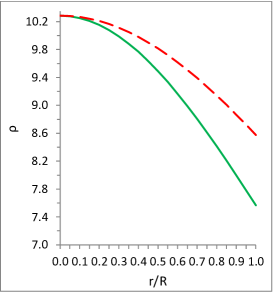
Figure 3: Variation of the density with radial coordinate $r/R$ are shown in figure. Here the legends are as follows: (i) $\rho$ is plotted with continuous line for Her X-1 (ii) $\rho$ is plotted with dashed line for white dwarf

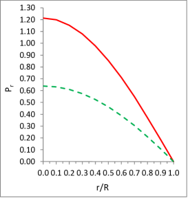
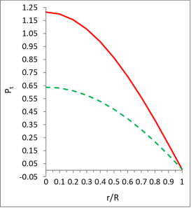
Figure 4: Variation of the density with radial coordinate $r/R$ are shown in figure. Here the legends are as follows: (i) $p_{r}$ is plotted with continuous line for Her X-1 and short-dashed line for white dwarf in left graph (left panel), (ii) $p_{t}$ is plotted with continuous line for Her X-1 and short-dashed line for white dwarf in right graph (right panel)

and

$$\frac{\kappa p_{r}}{C}=\frac{4(7-10Cr^{2}-C^{2}r^{4})}{7(1+Cr^{2})^{2}}\left[\frac{\psi_{pr}(1-\alpha+Cr^{2})^{3}+2\psi}{\psi(1-\alpha+Cr^{2})}\right]-\frac{8(Cr^{2}+3)}{7(1+Cr^{2})^{2}},$$ (20)

where

$$\psi_{pr}=\frac{A(1+Cr^{2})}{(1-\alpha+Cr^{2})^{4}\sqrt{(7-10Cr^{2}-Cr^{2})}}.$$ (21)

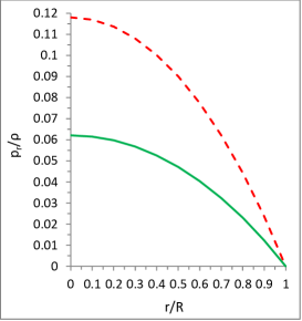
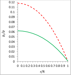
Figure 5: Variation of the density with radial coordinate $r/R$ are shown in figure. Here the legends are as follows: (i) $p_{r}/\rho$ is plotted with short-dashed line for Her X-1 and continuous line for white dwarf (left panel), (ii) $p_{t}/\rho$ is plotted with short-dashed line for Her X-1 and continuous line for white dwarf (right panel)

In the Figs. 3-5 we have plotted the nature of the above physical quantities which show viable features of the present model.

3.1 Matching condition

The above system of equations is to be solved subject to the boundary condition that radial pressure $p_{r}=0$ at $r=R$ (where $r=R$ is the outer boundary of the fluid sphere). It is clear that $m(r=R)=M$ is a constant and, in fact, the interior metric (2.1) can be joined smoothly at the surface of spheres ($r=R$), to an exterior Schwarzschild metric whose mass is same as above i.e. $m(r=R)=M$ Misner1964 .

The exterior spacetime of the star will be described by the Schwarzschild metric given by

$$ds^{2}=-\left(1-\frac{2M}{r}\right)^{-1}dr^{2}-r^{2}(d\theta^{2}+sin^{2}\theta d\phi^{2})+\left(1-\frac{2M}{r}\right)dt^{2}.$$ (22)

Continuity of the metric coefficients $g_{tt}$, $g_{rr}$ across the boundary surface $r=R$ between the interior and the exterior regions of the star yields the following conditions:

$$\left(1-\frac{2M}{R}\right)^{-1}=e^{\lambda(R)},$$ (23)

$$\left(1-\frac{2M}{r}\right)=\psi^{2}_{R},$$ (24)

where $\psi(r=R)=\psi_{R}$.

Equations (23) and (24) respectively give

$$M=\frac{R}{2}\left[\frac{8CR^{2}(3+CR^{2})}{7(1+CR^{2})^{2}}\right],$$ (25)

$$A=\frac{\sqrt{7-10CR^{2}-C^{2}R^{4}}}{\sqrt{7}(1+CR^{2})\psi_{\alpha R}(\frac{B}{A}-\Omega(R))}.$$ (26)

The radial pressure $p_{r}$ is zero at the boundary ($r=R$) provides

$$\frac{B}{A}=\frac{(1+CR^{2})\sqrt{7-10CR^{2}-C^{2}R^{2}}}{2(1-\alpha+CR^{2})^{3}[(1-\alpha+CR^{2})(3+CR^{2})-(7-10CR^{2}-C^{2}R^{4})]}\Omega(R),$$ (27)

where

$$\psi_{\alpha R}=(1-\alpha+CR^{2})^{2},$$ (28)

$$\Omega(R)=\frac{\{\psi_{\alpha 1}+\psi_{\alpha 2}(1-\alpha+CR^{2})+\psi_{\alpha 3}\psi_{\alpha R}\}\sqrt{\psi_{\alpha 5}-2(4+\alpha)(1-\alpha+CR^{2})-\psi_{\alpha R}}}{(1-\alpha+CR^{2})^{3}}+W(R),$$ (29)

$$W(R)=\frac{\psi_{\alpha 4}}{\sqrt{\psi_{\alpha 5}}}\log\left[\frac{\psi_{\alpha 5}-(4+\alpha)(1-\alpha+CR^{2})+\sqrt{\psi_{\alpha 5}}\sqrt{\psi_{\alpha 5}-2(4+\alpha)(1-\alpha+CR^{2})-\psi_{\alpha R}}}{(1-\alpha+CR^{2})\psi_{\alpha 5}}\right].$$ (30)

4 Some physical features of the model

4.1 Regularity at centre

The density $\rho$ and radial pressure $p_{r}$ and tangential pressure $p_{t}$ should be positive inside the star. The central density at centre for the present model is

$$\rho_{0}=\rho(r=0)=\frac{72C}{7}.$$ (31)

The metric Eq. (22) implies that $C=\frac{7\rho_{0}}{72}$ is positive finite.

Again, from Eq. (20), we obtain

$$\frac{p_{r}(r=0)}{C}=\frac{4A}{\sqrt{7}(1-\alpha)^{2}\psi_{r=0}}-\frac{24}{7},$$ (32)

where $p_{r}(r=0)>0$.

This immediately implies that

$$\frac{B}{A}<\frac{\sqrt{7}}{6(1-\alpha)^{4}}+\frac{\{\psi_{\alpha 1}+\psi_{\alpha 2}(1-\alpha)+\psi_{\alpha 3}(1-\alpha)^{2}\}\sqrt{\psi_{\alpha 5}-2(4+\alpha)(1-\alpha)-(1-\alpha)^{2}}}{(1-\alpha)^{3}}$$

$$+\frac{\psi_{\alpha 4}}{\sqrt{\psi_{\alpha 5}}}\log\left[\frac{\psi_{\alpha 5}-(4+\alpha)(1-\alpha)+\sqrt{\psi_{\alpha 5}}\sqrt{\psi_{\alpha 5}-2(4+\alpha)(1-\alpha)-(1-\alpha)^{2}}}{(1-\alpha)\psi_{\alpha 5}}\right].$$ (33)

4.2 Causality conditions

Inside the fluid sphere the speed of sound should be less than the speed of light i.e. $0\leq V_{sr}=\sqrt{\frac{dp_{r}}{d\rho}}<1$ and $0\leq V_{st}=\sqrt{\frac{dp_{t}}{d\rho}}<1$. Therefore

$${V^{2}}_{sr}=(1+Cr^{2})\left[\frac{4(C^{2}r^{4}+10Cr^{2}-7)(1+Cr^{2})(\psi_{r1}-\psi_{r2}-\psi_{r3})-8(Cr^{2}+5)}{8(C^{2}r^{4}+2Cr^{2}+25)}\right],$$ (34)

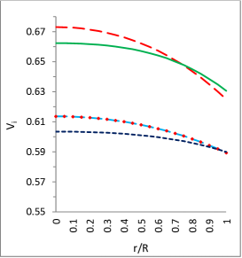
Figure 6: Variation of the sound velocity with radial coordinate $r/R$ are shown in figure. Here the legends are as follows: (i) $V_{r}$ is plotted with dash line for Her X-1, (ii) $V_{r}$ is plotted with marker continuous line for white dwarf (iii) $V_{t}$ is plotted with continuous line for Her X-1 (iv) $V_{t}$ is plotted with dotted line for white dwarf

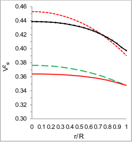
Figure 7: Variation of the sound velocity with radial coordinate r/R are shown in figure. Here the legends are as follows: (i) $V^{2}_{sr}$ is plotted with dotted line for Her X-1, (ii) $V^{2}_{sr}$ is plotted with dashed line for white dwarf (iii) $V^{2}_{st}$ is plotted with marker continuous line for Her X-1 (iv) $V^{2}_{st}$ is plotted with continuous line for white dwarf

$${V^{2}}_{st}=(1+Cr^{2})\left[\frac{4(C^{2}r^{4}+10Cr^{2}-7)(1+Cr^{2})(\psi_{r1}-\psi_{r2}-\psi_{r3})-8(Cr^{2}+5)-\psi_{r4}}{8(C^{2}r^{4}+2Cr^{2}+25)}\right],$$ (35)

where

$$\psi_{pr}=\frac{A(1+Cr^{2})}{(1-\alpha+Cr^{2})^{4}\sqrt{(7-10Cr^{2}-Cr^{2})}},$$ (36)

$$\psi_{r1}=[\frac{2}{(1-\alpha+Cr^{2})^{2}}+\frac{4(3-Cr^{2})(1-\alpha+Cr^{2})^{2}\psi_{pr}}{\psi(1+Cr^{2})(7-10Cr^{2}-C^{2}r^{4})}],$$ (37)

$$\psi_{r2}=[\frac{2K}{(1-\alpha+Cr^{2})}+\frac{(1-\alpha+Cr^{2})^{2}\psi_{pr}}{\psi}]^{2},$$ (38)

$$\psi_{r3}=\frac{8(3-Cr^{2})}{(7-10Cr^{2}-C^{2}r^{4})(1+Cr^{2})}[\frac{2}{(1-\alpha+Cr^{2})}+\frac{(1-\alpha+Cr^{2})^{2}\psi_{pr}}{\psi}],$$ (39)

$$\psi_{r4}=[4\alpha\frac{(1+Cr^{2})(1-\alpha+Cr^{2})\psi_{r5}-Cr^{2}\psi_{r6}(5-3\alpha+5Cr^{2})}{(1+Cr^{2})(1-\alpha+Cr^{2})^{3}}],$$ (40)

$$\psi_{r5}=[12C^{2}r^{4}+4(16-\alpha)Cr^{2}-(10\alpha+4)],$$ (41)

$$\psi_{r6}=[4C^{2}r^{4}+2(16-\alpha)Cr^{2}-(10\alpha+4)].$$ (42)

The physical quantities related to the above equations are plotted in Figs. 6 and 7.

4.3 Well behaved condition

The velocity of sound is monotonically decreasing away from the centre and it is increasing with the increase of density i.e. $\frac{d}{dr}(\frac{dp_{r}}{d\rho})<0$ or $(\frac{d^{2}p_{r}}{d\rho^{2}})>0$ and $\frac{d}{dr}(\frac{dp_{t}}{d\rho})<0$ or $(\frac{d^{2}p_{t}}{d\rho^{2}})>0$ for $0\leq r\leq R$. In this context it is worth mentioning that the equation of state at ultra-high distribution has the property that the sound speed is decreasing outwards Canuto1973 as can be observed from Fig. 6.

4.4 Energy conditions

The anisotropic fluid sphere composed of strange matter will satisfy the null energy condition (NEC), weak energy condition (WEC) and strong energy condition (SEC), if the following inequalities hold simultaneously at all points in the star:

NEC: $\rho\geq 0$,

WEC: $\rho+p_{r}\geq 0$,

WEC: $\rho+p_{t}\geq 0$,

SEC: $\rho+p_{r}+2p_{t}\geq 0$.

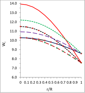
Figure 8: Variation of the energy conditions with radial coordinate $r/R$ are shown in figure. Here the legends are as follows: (i) $NEC$ is plotted with marker long-dashed line, $WEC_{r}$ with marker short-dashed line and $SEC$ with continuous line (for Her X-1), (ii) $NEC$ is plotted with marker continuous line, $WEC_{r}$ with long-dashed line and $SEC$ with short-dashed line (for white dwarf)

We have shown the energy conditions in Fig. 8 for Her X-1 under (i) and for white dwarf under (ii).

4.5 Stability conditions

4.5.1 Case-1:

In order to have an equilibrium configuration the matter must be stable against the collapse of local regions. This requires Le Chatelier s principle, also known as local or microscopic stability condition, that the radial pressure $p_{r}$ must be a monotonically non-decreasing function of $r$ such that $\frac{dp_{r}}{d\rho}\geq 0$ Bayin1982 . Heintzmann and Hillebrandt Heintzmann1975 also proposed that neutron star with anisotropic equation of state are stable for $\gamma>4/3$ as is observed from Fig. 9 and also shown in Tables 1 and 2 of our model related to compact stars.

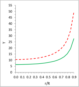
Figure 9: Variation of the adiabatic index with radial coordinate $r/R$ are shown in figure. Here the legends are as follows: (i) $\gamma$ is plotted with continuous line for Her X-1 (ii) $\gamma$ is plotted with dash line for white dwarf

4.5.2 Case-2:

For physically acceptable model, one expects that the velocity of sound should be within the range $0=V_{si}^{2}=(dp_{i}/d\rho)\leq 1$ Herrera1992 ; Abreu2007 . We plot the radial and transverse velocity of sound in Fig. 7 and conclude that all parameters satisfy the inequalities $0=V_{sr}^{2}=(dp_{i}/d\rho)\leq 1$ and $0=V_{st}^{2}=(dp_{i}/d\rho)\leq 1$ everywhere inside the star models. Also $0=V_{st}^{2}\leq 1$ and $0=V_{sr}^{2}\leq 1$, therefore $|V_{st}^{2}-V_{sr}^{2}|\leq 1$. Now, to examine the stability of local anisotropic fluid distribution, we follow the cracking (also known as overturning) concept of Herrera Herrera1992 which states that the region for which radial speed of sound is greater than the transverse speed of sound is a potentially stable region.

For this we calculate the difference of velocities as follows:

$$V_{st}^{2}-V_{sr}^{2}=\alpha\left[\frac{(1+Cr^{2})(1-\alpha+Cr^{2})\psi_{r5}-Cr^{2}\psi_{r6}(5-3\alpha+5Cr^{2})}{2(1+Cr^{2})^{3}(1-\alpha+Cr^{2})^{3}(C^{2}r^{4}+2Cr^{2}+25)}\right],$$ (43)

where

$$\psi_{r5}=[12C^{2}r^{4}+4(16-\alpha)Cr^{2}-(10\alpha+4)],$$ (44)

$$\psi_{r6}=[4C^{2}r^{4}+2(16-\alpha)Cr^{2}-(10\alpha+4)].$$ (45)

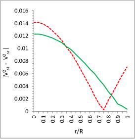
Figure 10: Variation of the absolute value of square of sound velocity with radial coordinate $r/R$ are shown in figure. Here the legends are as follows: (i) $|V^{2}_{st}-V^{2}_{sr}|$ is plotted with short-dashed line for Her X-1, (ii) $|V^{2}_{st}-V^{2}_{sr}|$ is plotted with continuous line for white dwarf

It can be seen that $|V_{st}^{2}-V_{sr}^{2}|$ at the centre lies between 0 and 1 (see Fig. 10). This implies that we must have $0\leq\frac{\alpha(10\alpha+4)}{50(1-\alpha)^{2}}\leq 1$. Then $\alpha$ should satisfy the following condition: $0\leq\alpha\leq\frac{52-\sqrt{704}}{40}$.

4.6 Generalized TOV equation

The generalized Tolman-Oppenheimer-Volkoff (TOV) equation

$$-\frac{M_{G}\left(\rho+p_{r}\right)}{r^{2}}e^{\frac{\lambda-\nu}{2}}-\frac{dp_{r}}{dr}+\frac{2}{r}\left(p_{t}-p_{r}\right)=0,$$ (46)

where $M_{G}=M_{G}(r)$ is the effective gravitational mass which can be given by

$$M_{G}(r)=\frac{1}{2}r^{2}e^{\frac{\nu-\lambda}{2}}\nu^{\prime}.$$ (47)

Substituting the value of $M_{G}(r)$ in Eq. (46), we get

$$-\frac{1}{2}\nu^{\prime}(\rho+p_{r})-\frac{dp_{r}}{dr}+\frac{2}{r}\left(p_{t}-p_{r}\right)=0.$$ (48)

Equation (48) basically describes the equilibrium condition for an anisotropic fluid subject to gravitational ($F_{g}$), hydrostatic ($F_{h}$) and anisotropic stress ($F_{a}$) which can, in a compact form, be expressed as

$$F_{g}+F_{h}+F_{a}=0,$$ (49)

where

$$F_{g}=-\frac{1}{2}\nu^{\prime}(\rho+p_{r}),$$ (50)

$$F_{h}=-\frac{dp_{r}}{dr},$$ (51)

$$F_{a}=\frac{2}{r}\left(p_{t}-p_{r}\right).$$ (52)

The above forces can be expressed in the following explicit forms:

$$F_{g}=-\frac{1}{2}\nu^{\prime}(\rho+p_{r})=\frac{C^{2}r}{8\pi}\left[\frac{8(6-2Cr^{2})}{7(1+Cr^{2})^{3}}\frac{[\psi_{pr}(1-\alpha+Cr^{2})^{3}+2\psi]}{\psi(1-\alpha+Cr^{2})}\right.$$

$$+\left.\frac{4(7-C^{2}r^{4}-10Cr^{2})}{7(1+Cr^{2})^{2}}\left(\frac{\psi_{pr}(1-\alpha+Cr^{2})^{3}+2\psi}{\psi(1-\alpha+Cr^{2})}\right)^{2}\right],$$ (53)

$$F_{h}=-\frac{dp_{r}}{dr}=\frac{C^{2}r}{4\pi}\left[\frac{4(C^{2}r^{4}+10Cr^{2}-7)}{7(1+Cr^{2})^{2}}(\psi_{r1}-\psi_{r2}-\psi_{r3})-\frac{8(Cr^{2}+5)}{7(1+Cr^{2})^{3}}\right],$$ (54)

$$F_{a}=\frac{2}{r}\left(p_{t}-p_{r}\right)=\frac{C^{2}r}{\pi}\left[\frac{2\alpha[(5\alpha+2)-(16-\alpha)Cr^{2}-2C^{2}r^{4}]}{7(1+Cr^{2})^{3}(1-\alpha+Cr^{2})^{2}}\right].$$ (55)

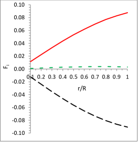
Figure 11: Variation of the forces with radial coordinate $r/R$ are shown in figure. Here the legends are as follows: $F_{g}$ is plotted with long-dashed line, $F_{h}$ with continuous line and $F_{a}$ with short-dashed line

Variation of different forces and attainment of equilibrium has been drawn in Fig. 11.

4.7 Effective mass-radius relation and surface redshift

Let us now turn our attention towards the effective mass to radius relationship. For static spherically symmetric perfect fluid star, Buchdahl Buchdahl1959 has proposed an absolute constraint on the maximally allowable mass-to-radius ratio ($M/R$) for isotropic fluid spheres as $2M/R\leq 8/9$ (in the unit $c=G=1$). This basically states that for a given radius a static isotropic fluid sphere cannot be arbitrarily massive. However, for more generalized expression for mass-to-radius ratio one may look at the paper by Mak and Harko Mak2003a .

For the present compact star model, the effective mass is written as

$$M_{eff}=4\pi\int_{0}^{R}\rho r^{2}dr=\frac{1}{2}R[1-e^{-\lambda(R)}]=\frac{1}{2}R\left[\frac{8CR^{2}(3+CR^{2})}{7(1+2CR^{2}+C^{2}R^{4})}\right].$$ (56)

The compactness of the star is therefore can be given by

$$u=\frac{M_{eff}}{R}=\frac{1}{2}\left[\frac{8CR^{2}(3+CR^{2})}{7(1+2CR^{2}+C^{2}R^{4})}\right].$$ (57)

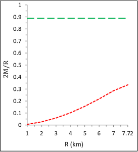
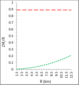
Figure 12: Variation of the mass with radial coordinate $r/R$ are shown in figure. Here the legends are as follows: (i) $2M/R$ is plotted with short-dashed line for Her X-1 and long-dashed line for its upper bound (left panel), (ii) $2M/R$ is plotted with short-dashed line for white dwarf and long-dashed line for its upper bound (right panel)

Therefore, the surface redshift ($Z$) corresponding to the above compactness factor ($u$) is obtained as

$$Z=[1-2u]^{-1/2}-1=[1-\frac{8CR^{2}(3+CR^{2})}{7(1+2CR^{2}+C^{2}R^{4})}]^{-1/2}-1.$$ (58)

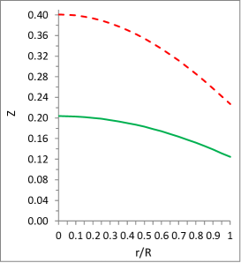
Figure 13: Variation of the redshift index radial coordinate $r/R$ are shown in figure. Here the legends are as follows: $Z$ is plotted with continuous line for Her X-1 and long-dashed line for white dwarf

We have shown the variation of physical quantities related to Buchdahl’s mass-to-radius ratio ($2M/R$) for isotropic fluid spheres and also surface redshift are plotted in Figs. 12 and 13.

5 Model parameters and comparison with some of the compact stars

In this Section we prepare several data sheets for the model parameters in the following Tables 1-3 and compare those with some of the compact stars, e.g. Strange star Her X-1 and White dwarf in Table 4. In our present investigation we propose a stable model with the parameters $R=12.5202$ Km and $M=0.8882~{}M_{\odot}$ (for white dwarf) whereas $R=7.7214$ Km and $M=0.8804$ $M_{\odot}$ (Her X-1) type compact star. The values of these data points have already been used for plotting graphs in the previous Sections 3 and 4 (See Figs. 1-13) in some way or others.

Table 1: Values of different physical parameters of White dwarf star for
 $\alpha=0.10$, $CR^{2}=0.068$, $M=0.8882$ $M_{\odot}$, $R=12.5202$ Km

$r$	$p_{r}$	$p_{t}$	$\rho$	$V_{r}$	$V_{t}$	$\Delta$	Z	$\gamma$
0.0	0.6386	0.6386	10.2857	0.6135	0.6034	0.00000	0.2036	10.4949
0.1	0.6314	0.6316	10.2663	0.6133	0.6033	0.00024	0.2028	10.5863
0.2	0.6096	0.6106	10.2084	0.6127	0.6031	0.00093	0.2003	10.8718
0.3	0.5738	0.5758	10.1129	0.6116	0.6026	0.0020	0.1961	11.3897
0.4	0.5245	0.5278	9.9814	0.6100	0.6019	0.0034	0.1903	12.2191
0.5	0.4624	0.4673	9.8157	0.6079	0.6010	0.0049	0.1830	13.5139
0.6	0.3885	0.3949	9.6185	0.6053	0.5997	0.0064	0.1741	15.5930
0.7	0.3040	0.3118	9.3926	0.6022	0.5980	0.0078	0.1637	19.2098
0.8	0.2101	0.2190	9.1412	0.5985	0.5959	0.0089	0.1519	26.6355
0.9	0.1083	0.1178	8.8676	0.5942	0.5932	0.0095	0.1388	49.2412
1.0	0.0000	0.0096	8.5754	0.5893	0.5899	0.0096	0.1244	$\infty$

Table 2: Values of different physical parameters of Strange star Her X-1 for
 $\alpha=0.11$, $CR^{2}=0.1178$, $M=0.8804$ $M_{\odot}$, $R=7.7214$ Km

$r$	$p_{r}$	$p_{t}$	$\rho$	$V_{r}$	$V_{t}$	$\Delta$	Z	$\gamma$
0.0	1.2135	1.2135	10.2857	0.6730	0.6624	0.0000	0.4010	4.2917
0.1	1.1984	1.1988	10.2521	0.6726	0.6622	0.0004	0.3991	4.3223
0.2	1.1533	1.1551	10.1523	0.6713	0.6617	0.0018	0.3933	4.4180
0.3	1.0795	1.0833	9.9890	0.6692	0.6607	0.0038	0.3838	4.5919
0.4	0.9790	0.9851	9.7665	0.6662	0.6592	0.0061	0.3707	4.8710
0.5	0.8546	0.8630	9.4906	0.6622	0.6571	0.0084	0.3541	5.3078
0.6	0.7096	0.7197	9.1681	0.6572	0.6541	0.0101	0.3342	6.0116
0.7	0.5475	0.5586	8.8067	0.6510	0.6501	0.0111	0.3113	7.2403
0.8	0.3725	0.3835	8.4143	0.6436	0.6450	0.0110	0.2856	9.7716
0.9	0.1886	0.1982	7.9990	0.6350	0.6385	0.0095	0.2574	17.4995
1.0	0.0000	0.0068	7.5686	0.6249	0.6305	0.0068	0.2271	-

Table 3: Values of the model parameters $A$, $B$, $C$ and $\alpha$ for different compact stars

Compact star	$M$	$R$	$A$	$B$	$C$	$\alpha$
candidates	($M_{\odot}$)	(Km)
White dwarf	0.8882	12.5202	-2.1463	0.5533	$4.3380\times 10^{-13}$	0.10
$Her~{}X-1$	0.8804	7.7214	-1.6255	0.5301	$1.9758\times 10^{-13}$	0.11

Table 4: Energy densities, central pressure and Buchdahl condition
for different compact star candidates for the above parameter values of Tables 1 - 3

Compact star	Central Density	Surface density	Central pressure	Buchdahl condition
candidates	($gm/cm^{-3}$)	($gm/cm^{-3}$)	($dyne/cm^{-2}$)	($2M/R\leq 8/9$)
White dwarf	$2.3961\times 10^{14}$	$2.0\times 10^{14}$	$1.3392\times 10^{34}$	0.1418
$Her~{}X-1$	$1.0913\times 10^{15}$	$0.8031\times 10^{15}$	$1.1591\times 10^{35}$	0.2280

Practically what we have done in the tables are as follows: In Tables 1-3 values of different physical parameters of Strange star Her X-1 and White dwarf have been provided. Under this data set then we calculate some physical parameters of compact star, say central density, surface density, central pressure etc in Table 4. It can be observed that these data are quite satisfactory for the compact stars whether it is strange star with central density $1.0913\times 10^{15}$ $gm/cm^{-3}$ or white dwarf with central density $2.3961\times 10^{14}$ $gm/cm^{-3}$. Likewise this feature of compact stars can be explored for some other physical parameters also.

6 Discussion and Conclusion

In the present work we have investigated about an anisotropic analogue of Durgapal-Fuloria Durgapal1985 and possibilities of interesting physical properties of the proposed model. As a necessary step we have contracted the anisotropic factor $\Delta$ by the help of both metric potentials $e^{\nu}$ and $e^{\lambda}$. However, $e^{\lambda}$ is considered here same as Durgapal-Fuloria Durgapal1985 whereas $e^{\nu}$ is that given by Lake Lake2003 .

The field equations are solved by the change of dependent variable method and under suitable boundary condition the interior metric (2.1) has been joined smoothly at the surface of spheres ($r=R$), to an exterior Schwarzschild metric whose mass is same as m$(r=R)=M$ Misner1964 . The solutions set thus obtained are correlated with the physical properties of some of the compact stars which include strange star as well as white dwarf. It is observed that the model is viable in connection to several physical features which are quite interesting and acceptable as proposed by other researchers within the framework of General Theory of Relativity.

As a detailed discussion we would like to put forward here that several verification scheme of the model have been performed and extract expected results some of which are as follows:

(1) Regularity at centre: The density $\rho$ and radial pressure $p_{r}$ and tangential pressure $p_{t}$ should be positive inside the star. It is shown that the central density at centre is $\rho_{0}=\rho(r=0)=\frac{72C}{7}$ and $p_{r}(r=0)>0$. This means that the density $\rho$ as well as radial pressure $p_{r}$ and tangential pressure $p_{t}$ all are positive inside the star.

(2) Causality conditions: It is shown that inside the fluid sphere the speed of sound is less than the speed of light i.e. $0\leq V_{sr}=\sqrt{\frac{dp_{r}}{d\rho}}<1$,  $0\leq V_{st}=\sqrt{\frac{dp_{t}}{d\rho}}<1$.

(3) Well behaved condition: The velocity of sound is monotonically decreasing away from the centre and it is increasing with the increase of density as can be observed from Fig. 6.

(4) Energy conditions: From Fig. 9 we observe that the anisotropic fluid sphere composed of strange matter satisfy the null energy condition (NEC), weak energy condition (WEC) and strong energy condition (SEC) simultaneously at all points in the star.

(5) Stability conditions: Following Heintzmann and Hillebrandt Heintzmann1975 we note that neutron star with anisotropic equation of state are stable for $\gamma>4/3$ as is observed in Tables 1 and 2 of our model. Also, it is expected that the velocity of sound should be within the range $0=V_{si}^{2}=(dp_{i}/d\rho)\leq 1$ Herrera1992 ; Abreu2007 . The plots for the radial and transverse velocity of sound in Fig. 7 everywhere inside the star models.

(6) Generalized TOV equation: The generalized Tolman-Oppenheimer-Volkoff equation describes the equilibrium condition for the anisotropic fluid subject to gravitational ($F_{g}$), hydrostatic ($F_{h}$) and anisotropic stress ($F_{a}$). Fig. 8 shows that the gravitational force is balanced by the joint action of hydrostatic and anisotropic forces to attain the required stability of the model. However, effect of anisotropic force is very less than the hydrostatic force.

(7) Effective mass-radius relation and surface redshift: For static spherically symmetric perfect fluid star, the Buchdahl Buchdahl1959 absolute constraint on the maximally allowable mass-to-radius ratio ($M/R$) for isotropic fluid spheres as $2M/R\leq 8/9=0.8888$ is seen to be maintained in the present model as can be observed from the Table 4.

In Sec. 5 we have made a comparative study by using model parameters and data of two of the compact stars which are, in general, very satisfactory as compared to the observational results. However, at this point we would like to comment that the sample data used for verifying the present model are to be increased to obtain more satisfactory and exhaustive features in the realm of physical reality.

References

- (1) M.C. Durgapal, R.S. Fuloria, Gen. Relativ. Gravit. 17, 671 (1985).
- (2) K. Lake, Phys. Rev. D 67, 104015 (2003).
- (3) Y.K. Gupta and S.K. Maurya, Astrophys. Space Sci. 331, 135 (2011).
- (4) M.H. Murad, S. Fatema, arXiv:1408.5126 (2014).
- (5) S.K. Maurya, Y.K. Gupta, S. Ray, arXiv: 1502.01915 [gr-qc] (2015).
- (6) R. Ruderman, Ann. Rev. Astron. Astrophys. 10, 427 (1972).
- (7) R. Bowers and E. Liang, Astrophys. J. 188, 657 (1974).
- (8) M.K. Mak and T. Harko, Proc. R. Soc. Lond. A 459, 393 (2002).
- (9) M.K. Mak and T. Harko, Proc. R. Soc. A 459, 393 (2003).
- (10) V.V. Usov, Phys. Rev. D 70, 067301 (2004).
- (11) V. Varela, F. Rahaman, S. Ray, K. Chakraborty and M. Kalam, Phys. Rev. D 82, 044052 (2010).
- (12) F. Rahaman, S. Ray, A. K. Jafry and K. Chakraborty, Phys. Rev. D 82, 104055 (2010).
- (13) F. Rahaman, P.K.F. Kuhfittig, M. Kalam, A.A. Usmani and S. Ray, Class. Quant. Grav. 28, 155021 (2011).
- (14) F. Rahaman, R. Maulick , A. K. Yadav, S. Ray and R. Sharma, Gen. Relativ. Gravit. 44, 107 (2012).
- (15) M. Kalam, F. Rahaman, S. Ray, Sk. Monowar Hossein, I. Karar and J. Naskar, Eur. Phys. J. C 72, 2248 (2012).
- (16) P. Bhar, F. Rahaman, S. Ray and V. Chatterjee, Eur. Phys. J. C 75, 190 (2015).
- (17) P.H. Nguyen and J.F. Pedraza, arXiv:1305.7220 [gr-qc] (2013).
- (18) P.H. Nguyen and M. Lingam, arXiv:1307.8433 [gr-qc] (2013).
- (19) M.K. Mak and T. Harko, Phys. Rev. D 70, 024010 (2004).
- (20) M.K. Mak and T. Harko, Int. J. Mod. Phys. D. 13, 149 (2004).
- (21) K. Lake, Phys. Rev. Lett. 92, 051101 (2004).
- (22) L. Herrera, J. Ospino and A. Di Parisco, Phys. Rev. D 77, 027502 (2008).
- (23) R.C. Tolman, Phys. Rev. 55, 364 (1939).
- (24) J.R. Oppenheimer, G.M. Volkoff, Phys. Rev. 55, 374 (1939).
- (25) D.D. Dionysiou, Astrophys. Space Sci. 85, 331 (1982).
- (26) C.W. Misner, D.H. Sharp, Phys. Rev. B 136, 571 (1964).
- (27) V. Canuto, In: Solvay Conf. on Astrophysics and Gravitation, Brussels (1973).
- (28) S.S. Bayin, Phys. Rev. D 26, 1262 (1982).
- (29) H. Heintzmann, W. Hillebrandt, Astron. Astrophys. 38, 51 (1975).
- (30) L. Herrera, Phys. Lett. A, 165 206, (1992).
- (31) H. Abreu, H. Hernandez and L. A. Nunez, Class. Quantum Gravit. 24, 4631 (2007).
- (32) H.A. Buchdahl, Phys. Rev. 116, 1027 (1959).
- (33) M.K. Mak and T. Harko, Proc. R. Soc. A 459, 393 (2003).