Deterministic Cramér-Rao Bound for Strictly Non-Circular Sources and Analytical Analysis of the Achievable Gains

Abstract

Recently, several high-resolution parameter estimation algorithms have been developed to exploit the structure of strictly second-order (SO) non-circular (NC) signals. They achieve a higher estimation accuracy and can resolve up to twice as many signal sources compared to the traditional methods for arbitrary signals. In this paper, as a benchmark for these NC methods, we derive the closed-form deterministic $R$-D NC Cramér-Rao bound (NC CRB) for the multi-dimensional parameter estimation of strictly non-circular (rectilinear) signal sources. Assuming a separable centro-symmetric $R$-D array, we show that in some special cases, the deterministic $R$-D NC CRB reduces to the existing deterministic $R$-D CRB for arbitrary signals. This suggests that no gain from strictly non-circular sources (NC gain) can be achieved in these cases. For more general scenarios, finding an analytical expression of the NC gain for an arbitrary number of sources is very challenging. Thus, in this paper, we simplify the derived NC CRB and the existing CRB for the special case of two closely-spaced strictly non-circular sources captured by a uniform linear array (ULA). Subsequently, we use these simplified CRB expressions to analytically compute the maximum achievable asymptotic NC gain for the considered two source case. The resulting expression only depends on the various physical parameters and we find the conditions that provide the largest NC gain for two sources. Our analysis is supported by extensive simulation results.

I Introduction

The problem of estimating the parameters of multi-dimensional ($R$-D) signals with $R\geq 1$, such as their directions of arrival, directions of departure, frequencies, and Doppler shifts, has been an extensive research area with widely-spread signal processing applications in radar, sonar, channel sounding, and wireless communications. Recently, various high-resolution parameter estimation algorithms such as NC MUSIC [1], NC Root-MUSIC [2], NC Standard ESPRIT [3], and NC Unitary ESPRIT [4, 5] have been developed to exploit the structure of signals from strictly second-order (SO) non-circular (NC) sources [6]. The term strictly SO NC (also called rectilinear) is based on the fact that the non-circularity coefficient of these signals is equal to one [6]. Examples of digital modulation schemes that use such signals include BPSK, PAM, and ASK. The aforementioned NC algorithms that exploit the non-circularity property are known to achieve a higher estimation accuracy and can resolve up to twice as many sources [5] compared to the traditional methods for arbitrary signals [7]. However, the “NC gain” achieved by these algorithms from estimating strictly non-circular sources has so far only been quantified through simulations. Hence, analytical expressions are highly desirable to study the properties of the NC gain under various conditions. As deriving a generic formulation for an arbitrary number of sources is very challenging, special cases can be considered to provide insights towards devising more general expressions. Based on the first-order performance analysis framework in [8], the scenario of a single strictly non-circular source for NC Standard ESPRIT was analyzed in [5]. It was found that no NC gain can be achieved in this case. A first attempt at analytically computing the NC gain of NC Standard ESPRIT for two uncorrelated strictly non-circular sources with maximum phase separation was taken in [9]. Despite the derivation of a closed-form expression for the NC gain, the considered assumptions in [9] are rather restrictive and do not provide the desired comprehensive insights.

The performance of high-resolution parameter estimation algorithms is often evaluated by comparing them to the deterministic (conditional) and stochastic (unconditional) Cramér-Rao bounds (CRBs) derived in [10] and [11], respectively. Whereas the stochastic data assumption requires both the signals and the noise to be complex Gaussian-distributed, the deterministic model assumes that the signals are arbitrary non-random sequences while only the noise follows a complex Gaussian distribution. Both CRBs are equally recognized in the literature. For the data model used to describe weak-sense non-circular sources whose non-circularity coefficient is between zero and one, a stochastic NC CRB has been derived in [12]. The follow-up papers [13] and [14] consider further variations of the underlying stochastic model assumption. The stochastic NC CRB in [12] was derived by extending the original Slepian-Bangs formula for circular complex Gaussian distributions [15] to weak-sense non-circular complex Gaussian distributions. However, this bound does not apply in the case of strict non-circularity, as in the weak-sense case, the real part and the imaginary part of the signal can be treated as independent random variables. This is not true for strictly non-circular sources, where the real and imaginary parts are linearly dependent.

In this paper, we derive a closed-form expression of the deterministic $R$-D NC CRB for strictly non-circular signals impinging on an arbitrary $R$-D sensor array. The derivation is based on the conventional Slepian-Bangs formula, which is still applicable due to the complex Gaussian noise assumption. Note that our initial contribution in [16] only states the 2-D result without providing a proof and further analysis. Based on the devised $R$-D NC CRB and assuming the $R$-D array to be separable and centro-symmetric, we show that in the special cases of equal rotation phases and full coherence of all strictly non-circular signals as well as for a single strictly non-circular source, the deterministic $R$-D NC CRB reduces to the existing deterministic $R$-D CRB for arbitrary signals [10]. This suggests that no NC gain from strictly non-circular sources can be achieved in these special cases. Note that the single source case of the $R$-D NC CRB has been analyzed in [5] for a uniform $R$-D array that contains a uniform linear array (ULA) in each mode. Here, we provide a generalization of this case to arbitrarily-formed (non-uniform) separable and centro-symmetric $R$-D arrays. Furthermore, the fact that twice as many sources can be resolved from the strictly non-circular data model is highlighted.

In our second contribution, we assume 1-D parameter estimation and simplify the derived deterministic NC CRB and the deterministic CRB for the special case of two closely-spaced strictly non-circular sources captured by a uniform linear array (ULA). These simplified expressions are subsequently used to analytically compute the maximum achievable NC gain, which only depends on the physical parameters, e.g., the number of sensors, the SNR, the correlation, the phase separation, and the location of the phase reference of the array. The devised expression is based on a truncated Taylor series expansion for closely-spaced sources. This is, however, the scenario, where high-resolution algorithms are primarily applied. Due to the fact that the NC gain expression is very general, the properties of the NC gain are studied in terms of the above-mentioned physical parameters. For instance, it is shown that the NC gain is largest if the sources are uncorrelated, the phase separation is maximum, and the phase reference is at the array centroid. Under these conditions, the two sources entirely decouple and do not influence each other.

The remainder of this paper is organized as follows: The data model is introduced in Section II. In Section III, the derivation of the deterministic $R$-D NC CRB is provided while its analysis is presented in Section IV. The asymptotic NC gain for two closely-spaced sources is analytically computed in Section V. Section VI illustrates and discusses the numerical results, and concluding remarks are drawn in Section VII.

Notation: We use italic letters for scalars, lower-case bold-face letters for column vectors, and upper-case bold-face letters for matrices. The superscripts ^T, ^∗, ^H, and ^-1 denote the transposition, complex conjugation, conjugate transposition, and the inversion of a matrix, respectively. The Hadamard product of two matrices $\bm{A}$ and $\bm{B}$ is represented by $\bm{A}\odot\bm{B}$, the Kronecker product is symbolized by $\bm{A}\otimes\bm{B}$, and the Khatri-Rao product (column-wise Kronecker product) is denoted by $\bm{A}\diamond\bm{B}$. The operator $\mathop{{\rm vec}}\left\{\bm{A}\right\}$ stacks the columns of the matrix $\bm{A}\in\mathbb{C}^{M\times N}$ into a column vector of length $MN\times 1$, the operator $\mathop{{\rm Tr}}\left\{\bm{A}\right\}$ returns the trace of the matrix $\bm{A}$, and $\mathrm{diag}\{\bm{a}\}$ returns a diagonal matrix with the elements of $\bm{a}$ placed on its diagonal. The matrix $\bm{\Pi}_{M}$ is the $M\times M$ exchange matrix with ones on its antidiagonal and zeros elsewhere. Also, the vector $\bm{1}_{M}$ denotes the $M\times 1$ vector of ones while $\bm{1}_{M\times M}$ is the $M\times M$ matrix of ones. Moreover, $\mathop{{\rm Re}}\left\{\cdot\right\}$ and $\mathop{{\rm Im}}\left\{\cdot\right\}$ extract the respective real and imaginary parts of a complex number or a matrix, $|\cdot|$ represents the absolute value of a complex number, and $\mathop{{\rm\mathbb{E}}}\left\{\cdot\right\}$ stands for the statistical expectation.

II Data Model

Let $N$ subsequent time instants of the measurement data sampled on an arbitrary separable $R$-D grid of size $M_{1}\times\ldots\times M_{R}$ be represented by a linear superposition of $d$ undamped exponentials in additive noise. The $t$-th time snapshot of the observed samples can be modeled as [17]

$$x_{m_{1},\ldots,m_{R}}(t)=\sum_{i=1}^{d}s_{i}(t)\prod_{r=1}^{R}{{\rm e}}^{\mathrm{j}k_{m_{r}}\mu^{({r})}_{i}}+n_{m_{1},\ldots,m_{R}}(t),$$ (1)

where $m_{r}=1,\ldots,M_{r}$, $t=1,\ldots,N$, $s_{i}(t)$ denotes the complex amplitude of the $i$-th undamped exponential at time instant $t$, and $k_{m_{r}}$ defines the sampling grid. Moreover, $\mu^{({r})}_{i}$ is the spatial frequency in the $r$-th mode with $i=1,\ldots,d$ and $r=1,\ldots,R$, and $n_{m_{1},\ldots,m_{R}}(t)$ contains the additive zero-mean circularly symmetric complex Gaussian noise samples with variance $\sigma_{\mathrm{n}}^{2}$.

In the array signal processing context, each of the $R$-D exponentials represents a narrow-band planar wavefront from stationary far-field sources and the complex amplitudes $s_{i}(t)$ are the source symbols. The objective is to estimate the $Rd$ spatial frequencies $\bm{\mu}_{i}=[\mu^{({1})}_{i},\ldots,\mu^{({R})}_{i}]^{\rm T},~{}\forall i$, from (1). We will also use the notation $\bm{\mu}^{({r})}=[\mu^{({r})}_{1},\ldots,\mu^{({r})}_{d}]^{\rm T},~{}\forall r,$ for the spatial frequencies of all sources in the $r$-th mode.

In order to obtain a more compact formulation of (1), we collect the observed samples into a measurement matrix $\bm{X}\in\mathbb{C}^{M\times N}$ with $M=\prod_{r=1}^{R}M_{r}$ by stacking the $R$ spatial dimensions along the rows and aligning the $N$ time snapshots as the columns. Subsequently, $\bm{X}$ can be modeled as

$$\bm{X}=\bm{A}\bm{S}+\bm{N}~{}\in\mathbb{C}^{M\times N},$$ (2)

where $\bm{S}\in\mathbb{C}^{d\times N}$ is the source symbol matrix and $\bm{N}\in\mathbb{C}^{M\times N}$ contains the noise samples. Furthermore, $\bm{A}=[\bm{a}(\bm{\mu}_{1}),\ldots,\bm{a}(\bm{\mu}_{d})]\in\mathbb{C}^{M\times d}$ is referred to as the array steering matrix, which consists of the array steering vectors $\bm{a}(\bm{\mu}_{i})$ defined by

$$\bm{a}(\bm{\mu}_{i})=\bm{a}^{(1)}\left(\mu_{i}^{(1)}\right)\otimes\cdots\otimes\bm{a}^{(R)}\left(\mu_{i}^{(R)}\right)\in\mathbb{C}^{M\times 1},$$ (3)

where $\bm{a}^{({r})}(\mu^{({r})}_{i})\in\mathbb{C}^{M_{r}\times 1}$ is the array steering vector of the $i$-th spatial frequency in the $r$-th mode. An alternative expression of $\bm{A}$ is given by

$$\bm{A}=\bm{A}^{(1)}\diamond\bm{A}^{(2)}\diamond\cdots\diamond\bm{A}^{(R)},$$ (4)

where $\bm{A}^{({r})}=[\bm{a}^{({r})}(\mu_{1}^{({r})}),\ldots,\bm{a}^{({r})}(\mu_{d}^{({r})})]\in\mathbb{C}^{M_{r}\times d}$ represents the array steering matrix in the $r$-th mode.

The non-circularity of a random variable can be defined through the non-circularity coefficient [6]. For every complex random variable $Z$ with zero mean, the non-circularity coefficient is given by

$$\kappa=\frac{\mathop{{\rm\mathbb{E}}}\left\{Z^{2}\right\}}{\mathop{{\rm\mathbb{E}}}\left\{|Z|^{2}\right\}}=|\kappa|{{\rm e}}^{\mathrm{j}\psi},\quad 0\leq|\kappa|\leq 1.$$ (5)

The cases $|\kappa|=0$ and $0<|\kappa|<1$ represent a circularly symmetric random variable and a weak-sense non-circular variable, respectively. The case $|\kappa|=1$ represents a strictly non-circular (strict sense or rectilinear) random variable. It can be shown that for $|\kappa|=1$, the real part and the imaginary part of $Z$ are linearly dependent [6], i.e., $c_{1}\cdot\mathop{{\rm Re}}\left\{Z\right\}=c_{2}\cdot\mathop{{\rm Im}}\left\{Z\right\}$ for constants $c_{1},c_{2}\in\real$.

In the context of array processing, the assumption of strictly SO non-circular sources requires that the complex symbol amplitudes of each source lie on a rotated line in the complex plane. This scenario is found, for instance, when real-valued data is transmitted by distinct sources causing different delays that result in different phase shifts. In this case, the symbol matrix $\bm{S}$ can be decomposed as [4]

$$\bm{S}=\bm{\Psi}\bm{S}_{0},$$ (6)

where $\bm{S}_{0}\in\mathbb{R}^{d\times N}$ is a real-valued symbol matrix and $\bm{\Psi}=\mathrm{diag}\{{{\rm e}}^{\mathrm{j}\varphi_{i}}\}_{i=1}^{d}$ contains stationary complex phase shifts on its diagonal that can be different for each source.

Using (6), the model (2) can be written as

$$\bm{X}=\bm{A}\bm{\Psi}\bm{S}_{0}+\bm{N}.$$ (7)

III Deterministic $R$-D NC Cramér-Rao Bound

In many applications, estimating the parameters of $R$-D signals with $R\geq 1$, can be of high importance. As a benchmark of such estimators, the corresponding CRBs for the multi-dimensional parameter estimation case are desirable. In this section, we first review the $R$-D CRB for arbitrary multi-dimensional signals and then derive the $R$-D NC CRB for multi-dimensional strictly non-circular signals. Additionally, we provide simplified expressions of the respective CRBs for the 1-D parameter estimation case.

III-A Deterministic $R$-D Cramér-Rao Bound

In the case of arbitrary signals, the set of parameters that needs to be considered for the deterministic $R$-D CRB is given by the angular parameters $\bm{\mu}=[\bm{\mu}^{({1})^{\rm T}},\ldots,\bm{\mu}^{({R})^{\rm T}}]^{\rm T}\in{}^{Rd\times 1}$, the real part and the imaginary part of the symbols $\bm{s}=\mathop{{\rm vec}}\left\{\bm{S}\right\}\in\mathbb{C}^{Nd\times 1}$, and the noise power $\sigma_{\mathrm{n}}^{2}$. For this parameter set that contains a total of $(2N+R)d+1$ parameters, the deterministic CRB matrix in the $R$-D parameter estimation case was derived in [10]. Its closed-form expression is given by

$$\bm{C}=\frac{\sigma_{\mathrm{n}}^{2}}{2N}\cdot\mathop{{\rm Re}}\left\{\left(\bm{D}^{\rm H}\bm{\Pi}^{\perp}_{\bm{A}}\bm{D}\right)\odot\hat{\bm{R}}^{({R})^{\rm T}}_{S}\right\}^{-1}\in{}^{Rd\times Rd},$$ (8)

where

$$\bm{\Pi}^{\perp}_{\bm{A}}=\bm{I}_{M}-\bm{A}\left(\bm{A}^{\rm H}\bm{A}\right)^{-1}\bm{A}^{\rm H}\in\mathbb{C}^{M\times M}$$ (9)

and

$$\bm{D}=\begin{bmatrix}\bm{D}^{({1})}&\cdots&\bm{D}^{({R})}\end{bmatrix}\in\mathbb{C}^{M\times Rd}$$ (10)

with $\bm{D}^{({r})}=[\bm{d}^{({r})}_{1},\ldots,\bm{d}^{({r})}_{d}]\in\mathbb{C}^{M\times d},~{}r=1,\ldots,R$, contains the partial derivatives of $\bm{A}$ with respect to the components of $\bm{\mu}_{i},~{}i=1,\ldots,d$, in the $r$-th mode. The vectors $\bm{d}^{({r})}_{i}$ are given by $\bm{d}^{({r})}_{i}=\partial\bm{a}(\bm{\mu}_{i})/\partial\mu^{({r})}_{i},~{}\forall i$. Writing $\bm{a}_{i}$ instead of $\bm{a}(\bm{\mu}_{i})$ to simplify the notation and using (3), we obtain

$$\bm{d}^{({r})}_{i}=\bm{a}_{i}^{(1)}\otimes\cdots\otimes\bm{a}_{i}^{(r-1)}\otimes\tilde{\bm{d}}^{({r})}_{i}\otimes\bm{a}_{i}^{(r+1)}\otimes\cdots\otimes\bm{a}_{i}^{(R)},$$ (11)

where $\tilde{\bm{d}}^{({r})}_{i}=\partial\bm{a}^{({r})}_{i}/\partial\mu_{i}^{({r})}$. Moreover, $\hat{\bm{R}}^{({R})}_{S}=\bm{1}_{R\times R}\otimes\hat{\bm{R}}_{S}$ contains the estimated signal covariance matrix $\hat{\bm{R}}_{S}=\bm{\Psi}^{*}\hat{\bm{R}}_{S_{0}}\bm{\Psi}$, where the real-valued sample covariance matrix $\hat{\bm{R}}_{S_{0}}$ is given by $\hat{\bm{R}}_{S_{0}}=\bm{S}_{0}\bm{S}_{0}^{\rm T}/N$. Note that $\hat{\bm{R}}_{S_{0}}$ can be written in matrix form as

$$\hat{\bm{R}}_{S_{0}} =\begin{bmatrix}\hat{P}_{1}&\hat{\rho}_{1,2}\sqrt{\hat{P}_{1}\hat{P}_{2}}&\ldots&\hat{\rho}_{1,d}\sqrt{\hat{P}_{1}\hat{P}_{d}}\\ \hat{\rho}_{2,1}\sqrt{\hat{P}_{1}\hat{P}_{2}}&\hat{P}_{2}&\ldots&\hat{\rho}_{2,d}\sqrt{\hat{P}_{2}\hat{P}_{d}}\\ \vdots&\vdots&\ddots&\vdots\\ \hat{\rho}_{d,1}\sqrt{\hat{P}_{1}\hat{P}_{d}}&\hat{\rho}_{d,2}\sqrt{\hat{P}_{2}\hat{P}_{d}}&\ldots&\hat{P}_{d}\end{bmatrix},$$

where $\hat{P}_{i}=\left\|\bm{s}_{0_{i}}\right\|_{2}^{2}/N$ is the empirical source power of the $i$-th source and $\bm{s}_{0_{i}}^{\rm T}\in{}^{1\times N}$ is the $i$-th row of $\bm{S}_{0}$. Furthermore, the empirical correlation coefficients $\hat{\rho}_{i,j}$ that represent the empirical correlation between the $i$-th and the $j$-th source vector are defined by

$$\hat{\rho}_{i,j}=\frac{1}{N}\cdot\frac{\bm{s}_{0_{i}}^{\rm T}\bm{s}_{0_{j}}}{\sqrt{\hat{P}_{1}\hat{P}_{2}}},~{}~{}\forall\;i\neq j,~{}~{}i,j=1,\ldots,d.$$ (12)

Note that $\bm{\hat{R}}_{S_{0}}$ is symmetric such that $\hat{\rho}_{i,j}=\hat{\rho}_{j,i}$.

In the special case of 1-D parameter estimation, the array steering matrix $\bm{A}$ reduces to $\bm{A}=[\bm{a}(\mu_{1}),\ldots,\bm{a}(\mu_{d})]\in\mathbb{C}^{M\times d}$ and the deterministic CRB matrix in (8) simplifies to

$$\bm{C}=\frac{\sigma_{\mathrm{n}}^{2}}{2N}\cdot\mathop{{\rm Re}}\left\{\left(\bm{D}^{\rm H}\bm{\Pi}^{\perp}_{\bm{A}}\bm{D}\right)\odot\hat{\bm{R}}_{S}^{\rm T}\right\}^{-1}\in{}^{d\times d},$$ (13)

where $\bm{D}$ becomes

$$\bm{D}=\begin{bmatrix}\bm{d}_{1}&\cdots&\bm{d}_{d}\end{bmatrix}\in\mathbb{C}^{M\times d}$$ (14)

with $\bm{d}_{i}=\partial\bm{a}(\mu_{i})/\partial\mu_{i},~{}\forall\;i$.

III-B Deterministic $R$-D NC Cramér-Rao Bound

In contrast to the case of arbitrary signals, the set of parameters for the strictly non-circular source model in (7) is given by the angular parameters $\bm{\mu}\in{}^{Rd\times 1}$, the real-valued symbols $\bm{s}_{0}=\mathop{{\rm vec}}\left\{\bm{S}_{0}\right\}\in{}^{Nd\times 1}$, the rotation phase angles $\bm{\varphi}\in{}^{d\times 1}$, and the noise power $\sigma_{\mathrm{n}}^{2}$. Thus, the number of parameters is now equal to $(N+R+1)d+1$, which requires the derivation of a new CRB for this parameter set.

The resulting closed-form expression for the deterministic NC CRB matrix $\bm{C}^{({\rm nc})}$ in the $R$-D case is stated in the following theorem:

Theorem 1.

The $R$-D deterministic NC CRB matrix $\bm{C}^{({\rm nc})}$ for strictly non-circular sources is given by

$$\bm{C}^{({\rm nc})}=\frac{\sigma_{\mathrm{n}}^{2}}{2N}\cdot\Big{\{}\left(\bm{G}_{2}-\bm{G}_{1}\bm{G}_{0}^{-1}\bm{G}_{1}^{\rm T}\right)\odot\hat{\bm{R}}^{({R})}_{S_{0}}$$

$$+\left[\left(\bm{G}_{1}\bm{G}_{0}^{-1}\bm{H}_{0}\right)\odot\hat{\bm{R}}^{({R})}_{S_{0}}\right]\!\left[\left(\bm{G}_{0}-\bm{H}_{0}^{\rm T}\bm{G}_{0}^{-1}\bm{H}_{0}\right)\odot\hat{\bm{R}}^{({R})}_{S_{0}}\right]^{-1}$$

$$\cdot\left[\left(\bm{H}_{1}^{\rm T}-\bm{H}_{0}^{\rm T}\bm{G}_{0}^{-1}\bm{G}_{1}^{\rm T}\right)\odot\hat{\bm{R}}^{({R})}_{S_{0}}\right]+\left[\bm{H}_{1}\odot\hat{\bm{R}}^{({R})}_{S_{0}}\right]$$

$$\cdot\left[\bm{G}_{0}\odot\hat{\bm{R}}^{({R})}_{S_{0}}\right]^{-1}\!\!\cdot\left[\left(\bm{H}_{0}^{\rm T}\bm{G}_{0}^{-1}\bm{G}_{1}^{\rm T}\right)\odot\hat{\bm{R}}^{({R})}_{S_{0}}\right]+\left[\bm{H}_{1}\odot\hat{\bm{R}}^{({R})}_{S_{0}}\right]$$

$$\cdot\left[\bm{G}_{0}\odot\hat{\bm{R}}^{({R})}_{S_{0}}\right]^{-1}\cdot\left[\left(\bm{H}_{0}^{\rm T}\bm{G}_{0}^{-1}\bm{H}_{0}\right)\odot\hat{\bm{R}}^{({R})}_{S_{0}}\right]$$

$$\cdot\left[\left(\bm{G}_{0}-\bm{H}_{0}^{\rm T}\bm{G}_{0}^{-1}\bm{H}_{0}\right)\odot\hat{\bm{R}}^{({R})}_{S_{0}}\right]^{-1}\!\!\!\cdot\!\left[\left(\bm{H}_{0}^{\rm T}\bm{G}_{0}^{-1}\bm{G}_{1}^{\rm T}\right)\odot\hat{\bm{R}}^{({R})}_{S_{0}}\right]$$

$$-\left[\bm{H}_{1}\odot\hat{\bm{R}}^{({R})}_{S_{0}}\right]\cdot\left[\left(\bm{G}_{0}-\bm{H}_{0}^{\rm T}\bm{G}_{0}^{-1}\bm{H}_{0}\right)\odot\hat{\bm{R}}^{({R})}_{S_{0}}\right]^{-1}$$

$$\cdot\left[\bm{H}_{1}^{\rm T}\odot\hat{\bm{R}}^{({R})}_{S_{0}}\right]\Big{\}}^{-1}\in{}^{Rd\times Rd},$$ (15)

where $\hat{\bm{R}}^{({R})}_{S_{0}}=\bm{1}_{R\times R}\otimes\hat{\bm{R}}_{S_{0}}$ and the matrices $\bm{G}_{n}$ and $\bm{H}_{n},~{}n=0,1,2$, are defined as

$$\bm{G}_{0} =\mathop{{\rm Re}}\left\{\bm{\Psi}^{*}\bm{A}^{\rm H}\bm{A}\bm{\Psi}\right\}\in{}^{d\times d},$$ (16)

$$\bm{H}_{0} =\mathop{{\rm Im}}\left\{\bm{\Psi}^{*}\bm{A}^{\rm H}\bm{A}\bm{\Psi}\right\}\in{}^{d\times d},$$ (17)

$$\bm{G}_{1} =\mathop{{\rm Re}}\left\{(\bm{I}_{R}\otimes\bm{\Psi}^{*})\bm{D}^{\rm H}\bm{A}\bm{\Psi}\right\}\in{}^{Rd\times d},$$ (18)

$$\bm{H}_{1} =\mathop{{\rm Im}}\left\{(\bm{I}_{R}\otimes\bm{\Psi}^{*})\bm{D}^{\rm H}\bm{A}\bm{\Psi}\right\}\in{}^{Rd\times d},$$ (19)

$$\bm{G}_{2} =\mathop{{\rm Re}}\left\{(\bm{I}_{R}\otimes\bm{\Psi}^{*})\bm{D}^{\rm H}\bm{D}(\bm{I}_{R}\otimes\bm{\Psi})\right\}\in{}^{Rd\times Rd}$$ (20)

and $\bm{A}$ and $\bm{D}$ are given by (4) and (10), respectively.

Proof:

The proof is given in Appendix A. ∎

It should be highlighted that the assumption of the $R$-D array to be separable is not required for the derivation of (15) in Appendix A. In fact, (15) is valid for arbitrarily formed $R$-D arrays, where the columns of $\bm{A}$ and $\bm{D}$ are represented accordingly. However, the separability assumption simplifies the further analysis and helps with the presentation of our results in the following sections.

In analogy to the 1-D parameter estimation case of the CRB for arbitrary signals in (13), the deterministic 1-D NC CRB matrix is stated in the corollary:

Corollary 1.

The deterministic 1-D NC CRB is given by (15), where $\hat{\bm{R}}^{({R})}_{S_{0}}$ reduces to $\hat{\bm{R}}_{S_{0}}$ and $\bm{G}_{1}$, $\bm{H}_{1}$, and $\bm{G}_{2}$ simplify to

$$\bm{G}_{1} =\mathop{{\rm Re}}\left\{\bm{\Psi}^{*}\bm{D}^{\rm H}\bm{A}\bm{\Psi}\right\}\in{}^{d\times d},$$ (21)

$$\bm{H}_{1} =\mathop{{\rm Im}}\left\{\bm{\Psi}^{*}\bm{D}^{\rm H}\bm{A}\bm{\Psi}\right\}\in{}^{d\times d},$$ (22)

$$\bm{G}_{2} =\mathop{{\rm Re}}\left\{\bm{\Psi}^{*}\bm{D}^{\rm H}\bm{D}\bm{\Psi}\right\}\in{}^{d\times d}$$ (23)

with $\bm{A}$ and $\bm{D}$ being defined in (13) and in (14).

IV Analysis of the Deterministic $R$-D NC CRB

In this section, we discuss interesting special cases and properties of the derived $R$-D NC CRB, where the $R$-D array is assumed to be separable and centro-symmetric for simplicity. Specifically, we investigate the two cases of equal rotation phases and full coherence for an arbitrary number of strictly non-circular signals before we focus on the single source case ($d=1$). It is shown that in these special cases, the deterministic $R$-D NC CRB reduces to the $R$-D CRB. Furthermore, we also analyze the maximum number of resolvable NC sources.

For our analysis, we first refine the model in (7). Assuming the $R$-D array to be centro-symmetric, i.e., it is symmetric with respect to its centroid, its array steering matrices $\bm{A}^{({r})}$ from (4) satisfy [18]

$$\bm{\Pi}_{M_{r}}\bm{A}^{({r})^{*}}=\bm{A}^{({r})}\bm{\Delta}^{({r})}_{\mathrm{c}}~{}~{}\forall\;r,$$ (24)

where $\bm{\Delta}^{({r})}_{\mathrm{c}}\in\mathbb{C}^{d\times d}$ is a unitary diagonal matrix that depends on the phase reference. If the $r$-mode array centroid is chosen as the phase reference [18], we have $\bm{\Delta}^{({r})}_{\mathrm{c}}=\bm{I}_{d}$. The phase reference $\delta^{({r})}$ along the $r$-th mode can be defined by

$$\delta^{({r})}=\frac{1}{M_{r}}\sum_{m_{r}=1}^{M_{r}}k_{m_{r}}.$$ (25)

Note that $\delta^{({r})}$ is a property of the array and independent of $\mu^{({r})}_{i}$. Using (24) and (25), we can decompose the $r$-mode array steering matrix $\bm{A}^{({r})}$ with an arbitrary phase reference along the $r$-th mode as

$$\bm{A}^{({r})}=\bar{\bm{A}}^{({r})}\bm{\Delta}^{({r})}.$$ (26)

The matrix $\bar{\bm{A}}\in\mathbb{C}^{M_{r}\times d}$ is the array steering matrix whose phase reference is located at the centroid of the $r$-th mode such that for $\bar{\bm{A}}^{({r})}$, from (24), the identity $\bar{\bm{A}}^{({r})}=\bm{\Pi}_{M_{r}}\bar{\bm{A}}^{({r})^{*}}$ holds. Furthermore, the diagonal matrix $\bm{\Delta}^{({r})}=\mathrm{diag}\big{\{}{\rm e}^{\mathrm{j}\delta^{({r})}\mu^{({r})}_{i}}\big{\}}_{i=1}^{d}$ contains the shifts of the phase reference for each $\mu^{({r})}_{i}$. By inserting (26) into (24), we can easily establish the relation $\bm{\Delta}^{({r})}_{\mathrm{c}}=\bm{\Delta}^{({r})^{*}}\bm{\Delta}^{({r})^{*}}$. Thus, if the actual phase reference is at the array centroid of the $r$-th mode, we have $\delta^{({r})}=0$, $\bm{\Delta}^{({r})}=\bm{\Delta}^{({r})}_{\mathrm{c}}=\bm{I}_{d}$, and consequently $\bm{A}^{({r})}=\bar{\bm{A}}^{({r})}$.

Based on (26), we can rewrite $\bm{A}$ in (4) as

$$\bm{A} =\left(\bar{\bm{A}}^{(1)}\bm{\Delta}^{(1)}\right)\diamond\left(\bar{\bm{A}}^{(2)}\bm{\Delta}^{(2)}\right)\diamond\cdots\diamond\left(\bar{\bm{A}}^{(R)}\bm{\Delta}^{(R)}\right)$$

$$=\bar{\bm{A}}\bm{\Delta},$$ (27)

where $\bar{\bm{A}}=\bar{\bm{A}}^{(1)}\diamond\bar{\bm{A}}^{(2)}\diamond\cdots\diamond\bar{\bm{A}}^{(R)}\in\mathbb{C}^{M\times d}$ and $\bm{\Delta}=\bm{\Delta}^{(1)}\cdot\bm{\Delta}^{(2)}\cdot\ldots\cdot\bm{\Delta}^{(R)}\in\mathbb{C}^{d\times d}$.

Inserting (27) into the expression for strictly non-circular signals in (7), we obtain

$$\bm{X}=\bar{\bm{A}}\bm{\Delta}\bm{\Psi}\bm{S}_{0}+\bm{N}=\bar{\bm{A}}\bm{\Phi}\bm{S}_{0}+\bm{N},$$ (28)

where we have defined $\bm{\Phi}=\bm{\Delta}\bm{\Psi}=\mathop{{\rm diag}}\left\{{\rm e}^{\mathrm{j}(\varphi_{i}+\delta_{i})}\right\}_{i=1}^{d}$ with $\delta_{i}=\sum_{r=1}^{R}\delta^{({r})}\mu^{({r})}_{i}$.

IV-A Sources with Equal Phases

An interesting special case of the model (27) occurs when the phase references in each of the $R$ modes coincide with the centroid of the $R$-D array, i.e., $\delta^{({r})}=0~{}\forall\;r$ such that $\bm{\Delta}=\bm{I}_{d}$ and $\bm{A}=\bar{\bm{A}}$, and, at the same time, the rotation phase angles for all $d$ sources are the same, i.e., $\varphi_{i}=\varphi~{}\forall\;i$. Hence, we have

$$\bm{\Phi}=\bm{\Psi}={\rm e}^{\mathrm{j}\varphi}\bm{I}_{d}.$$ (29)

Under these assumptions, the matrices $\bm{G}_{n}$, $n=0,1,2$, can be expressed as

$$\bm{G}_{0} =\mathop{{\rm Re}}\left\{{\rm e}^{-\mathrm{j}\varphi}\bm{I}_{d}\bm{A}^{\rm H}\bm{{A}}\bm{{I}}_{d}{\rm e}^{\mathrm{j}\varphi}\right\}=\mathop{{\rm Re}}\left\{\bm{{A}}^{\rm H}\bm{{A}}\right\}=\bm{{A}}^{\rm H}\bm{{A}}$$

$$\bm{{G}}_{1} =\mathop{{\rm Re}}\left\{{\rm e}^{-\mathrm{j}\varphi}\bm{{I}}_{Rd}\bm{D}^{\rm H}\bm{{A}}\bm{{I}}_{d}{\rm e}^{\mathrm{j}\varphi}\right\}=\mathop{{\rm Re}}\left\{\bm{D}^{\rm H}\bm{{A}}\right\}=\bm{D}^{\rm H}\bm{A}$$

$$\bm{{G}}_{2} =\mathop{{\rm Re}}\left\{{\rm e}^{-\mathrm{j}\varphi}\bm{{I}}_{Rd}\bm{D}^{\rm H}\bm{D}\bm{{I}}_{Rd}{\rm e}^{\mathrm{j}\varphi}\right\}=\mathop{{\rm Re}}\left\{\bm{D}^{\rm H}\bm{D}\right\}=\bm{D}^{\rm H}\bm{D}$$

while the matrices $\bm{{H}}_{n}$ evaluate to zero. The proof that the matrices $\bm{A}^{\rm H}\bm{A}\in{}^{d\times d}$, $\bm{D}^{\rm H}\bm{A}\in{}^{Rd\times d}$, and $\bm{D}^{\rm H}\bm{D}\in{}^{Rd\times Rd}$ are real-valued can be found in Appendix B.

Using these observations, all terms in (15) containing $\bm{{H}}_{0}$ or $\bm{{H}}_{1}$ vanish and the $R$-D NC CRB matrix simplifies to

$$\bm{C}^{({\rm nc})} =\frac{\sigma_{\mathrm{n}}^{2}}{2N}\cdot\Big{\{}\left(\bm{G}_{2}-\bm{G}_{1}\bm{G}_{0}^{-1}\bm{G}_{1}^{\rm T}\right)\odot\hat{\bm{R}}^{(R)}_{S_{0}}\Big{\}}^{-1}$$

$$=\frac{\sigma_{\mathrm{n}}^{2}}{2N}\cdot\bigg{\{}\big{(}\bm{D}^{\rm H}\bm{\Pi}_{\bm{A}}^{\perp}\bm{D}\big{)}\odot\hat{\bm{R}}_{S}^{(R)^{\rm T}}\bigg{\}}^{-1}$$

$$=\bm{C},$$ (30)

where we have used the fact that $\hat{\bm{R}}^{(R)}_{S}=\hat{\bm{R}}^{(R)}_{S_{0}}=\hat{\bm{R}}_{S_{0}}^{(R)^{\rm T}}$ for $\bm{\Psi}={\rm e}^{\mathrm{j}\varphi}\bm{I}_{d}$. From (30), it is evident that the $R$-D NC CRB reduces to the $R$-D CRB if the phase reference is at the $R$-D array centroid and the rotation phase angles of the sources are equal. This suggests that no gain from strictly non-circular sources can be achieved in this case.

IV-B Coherent Sources

In this section, the case of full coherence is discussed, i.e., the correlation coefficients $\hat{\rho}_{i,j}$ between all pairs of sources are given by $|\hat{\rho}_{i,j}|=1~{}\forall\;i,j$. For simplicity, we assume that all the sources have unit power, i.e., $\hat{P}_{i}=1~{}\forall\;i$. Under these assumptions, the sample covariance matrix takes the form $\hat{\bm{R}}_{S_{0}}=\bm{1}_{d\times d}$ such that $\hat{\bm{R}}^{({R})}_{S_{0}}=\bm{1}_{Rd\times Rd}$. Hence, all the Hadamard products with $\hat{\bm{R}}^{({R})}_{S_{0}}$ in the $R$-D NC CRB matrix in (15) can be omitted and the remaining parts are arranged in the following form

$$\!\!\!\frac{\sigma_{\mathrm{n}}^{2}}{2N}\cdot\bm{C}^{({\rm nc})^{-1}}\!\!=\bm{{G}}_{2}-\bm{{G}}_{1}\!\left[\bm{{G}}_{0}^{-1}+\bm{{G}}_{0}^{-1}\bm{{H}}_{0}\tilde{\bm{G}}^{-1}\bm{{H}}_{0}^{\rm T}\bm{{G}}_{0}^{-1}\right]\bm{{G}}_{1}^{\rm T}$$

$$~{}~{}~{}+\bm{{H}}_{1}\bm{{G}}_{0}^{-1}\bm{{H}}_{0}^{\rm T}\left[\bm{{G}}_{0}^{-1}+\bm{{G}}_{0}^{-1}\bm{{H}}_{0}\tilde{\bm{G}}^{-1}\bm{{H}}_{0}^{\rm T}\bm{{G}}_{0}^{-1}\right]\bm{{G}}_{1}^{\rm T}$$

$$~{}~{}~{}+\bm{{G}}_{1}\bm{{G}}_{0}^{-1}\bm{{H}}_{0}\tilde{\bm{G}}^{-1}\bm{{H}}_{1}^{\rm T}-\bm{{H}}_{1}\tilde{\bm{G}}^{-1}\bm{{H}}_{1}^{\rm T}$$ (31)

$$=\bm{{G}}_{2}-\left(\bm{{G}}_{1}-\bm{{H}}_{1}\bm{{G}}_{0}^{-1}\bm{{H}}_{0}^{\rm T}\right)\left(\bm{{G}}_{0}-\bm{{H}}_{0}\bm{{G}}_{0}^{-1}\bm{{H}}_{0}^{\rm T}\right)^{-1}\bm{{G}}_{1}^{\rm T}$$

$$~{}~{}~{}-\left(\bm{{H}}_{1}-\bm{{G}}_{1}\bm{{G}}_{0}^{-1}\bm{{H}}_{0}\right)\!\left(\bm{{G}}_{0}-\bm{{H}}_{0}^{\rm T}\bm{{G}}_{0}^{-1}\bm{{H}}_{0}\right)^{-1}\!\!\bm{{H}}_{1}^{\rm T},$$ (32)

where in (31), we have defined $\tilde{\bm{G}}=\bm{G}_{0}-\bm{H}_{0}^{\rm T}\bm{G}_{0}^{-1}\bm{H}_{0}$ and replaced the terms in the square brackets by applying the converse of the matrix inversion lemma, yielding the matrix $(\bm{G}_{0}-\bm{H}_{0}\bm{G}_{0}^{-1}\bm{H}_{0}^{\rm T})^{-1}$. Note that (32) can be transformed into the block matrix form

$$\frac{\sigma_{\mathrm{n}}^{2}}{2N}\cdot\bm{C}^{({\rm nc})^{-1}} =\bm{{G}}_{2}-\begin{bmatrix}\bm{{G}}_{1}&\bm{{H}}_{1}\end{bmatrix}\begin{bmatrix}\bm{{G}}_{0}&\bm{{H}}_{0}\\ \bm{{H}}_{0}^{\rm T}&\bm{{G}}_{0}\end{bmatrix}^{-1}\begin{bmatrix}\bm{{G}}_{1}^{\rm T}\\ \bm{{H}}_{1}^{\rm T}\end{bmatrix},$$

which represents a very interesting simplification of the original expression.

In the next step, we rewrite the $R$-D CRB matrix for arbitrary signals in (8) for the case of coherent sources in a similar form. Under the aforementioned assumptions, the $R$-D sample covariance matrix is given by $\hat{\bm{R}}^{({R})}_{S}=\bm{1}_{R\times R}\otimes(\bm{\Psi}^{*}\bm{1}_{d\times d}\bm{\Psi})=(\bm{I}_{R}\otimes\bm{\Psi}^{*})\bm{1}_{Rd\times Rd}(\bm{I}_{R}\otimes\bm{\Psi})$. Hence, we simplify the original form of the CRB in (13) into

$$\frac{\sigma_{\mathrm{n}}^{2}}{2N}\cdot\bm{C}^{-1}\!=\mathrm{Re}\Big{\{}\!\big{(}\bm{D}^{\rm H}\bm{\Pi}^{\perp}_{\bm{A}}\bm{D}\big{)}\Big{.}$$

$$\Big{.}\quad\quad\quad\quad\quad\quad\quad\odot\big{(}(\bm{I}_{R}\otimes\bm{\Psi}^{*})\bm{1}_{Rd\times Rd}(\bm{I}_{R}\otimes\bm{\Psi})\big{)}\!\Big{\}}$$ (33)

$$=\mathrm{Re}\Big{\{}(\bm{I}_{R}\otimes\bm{\Psi}^{*})\bm{D}^{\rm H}\bm{D}(\bm{I}_{R}\otimes\bm{\Psi})-(\bm{I}_{R}\otimes\bm{\Psi}^{*})\bm{D}^{\rm H}\bm{A}\bm{\Psi}\Big{.}$$

$$\Big{.}\quad\quad\quad\quad\quad~{}\cdot\left(\bm{\Psi}^{*}\bm{A}^{\rm H}\bm{A}\bm{\Psi}\right)^{-1}\bm{\Psi}^{*}\bm{A}^{\rm H}\bm{D}(\bm{I}_{R}\otimes\bm{\Psi})\Big{\}}$$ (34)

$$=\mathrm{Re}\Big{\{}\bm{{G}}_{2}+\mathrm{j}\bm{{H}}_{2}-\left(\bm{{G}}_{1}+\mathrm{j}\bm{{H}}_{1}\right)\Big{.}$$

$$\Big{.}\quad\quad\quad\quad\quad~{}\cdot\left(\bm{{G}}_{0}+\mathrm{j}\bm{{H}}_{0}\right)^{-1}(\bm{{G}}_{1}^{\rm T}-\mathrm{j}\bm{{H}}_{1}^{\rm T})\Big{\}},$$ (35)

where we have introduced additional matrices $\bm{\Psi}$ in (34) by noting that $\bm{\Psi}\bm{\Psi}^{*}=\bm{I}_{d}$. To proceed we require the following lemma:

Lemma 1.

The inverse of a full rank complex-valued matrix $\bm{C}=\bm{A}+\mathrm{j}\bm{B}\in\mathbb{C}^{n\times n}$ with the real part $\bm{A}\in{}^{n\times n}$ and the imaginary part $\bm{B}\in{}^{n\times n}$ can be split into its real part and its imaginary part as follows:

$$\bm{C}^{-1} =\left(\bm{{A}}+\bm{{B}}\bm{{A}}^{-1}\bm{{B}}\right)^{-1}-\mathrm{j}\bm{{A}}^{-1}\bm{{B}}\left(\bm{{A}}+\bm{{B}}\bm{{A}}^{-1}\bm{{B}}\right)^{-1}$$

if $\bm{A}$ and $\left(\bm{A}+\bm{B}\bm{A}^{-1}\bm{B}\right)$ are invertible.

Proof:

To prove this lemma, it is sufficient to multiply $\bm{C}$ with $\bm{C}^{-1}$ and show that the result is the identity matrix. ∎

Applying Lemma 1 to (35), we split $\bm{C}^{-1}$ into its real and imaginary part. After some elementary operations and using the fact that $\bm{H}_{0}^{\rm T}=-\bm{H}_{0}$, we obtain equation (32) and consequently, we have $\bm{C}^{({\rm nc})}=\bm{C}$. Thus, both $R$-D CRBs become equal if all the sources are coherent. Note that this result is valid for arbitrary $R$-D arrays as the assumptions of separability and centro-symmetry were not used in the derivation. Analogously to the special case considered in the previous subsection, our findings suggests that no NC gain can be achieved for coherent sources.

IV-C Single Source Case

The expression for the deterministic $R$-D NC CRB is formulated in terms of the matrices $\bm{A}$, $\bm{\Psi}$, $\bm{D}$, and the sample covariance matrix $\hat{\bm{R}}_{S_{0}}$. Consequently, it provides no explicit insights into the parameters of physical significance, e.g., the number of sensors $M$, the correlation coefficient $\rho$, the source separation. Knowing how the CRB scales with these parameters can facilitate array design decisions on the number of required sensors to achieve a certain performance under specific conditions. As establishing a generic formulation for an arbitrary number of sources is very challenging, we can, however, consider special cases such as the single source case. Note that this scenario of the $R$-D NC CRB has been analyzed in [5] for a uniform $R$-D array containing a uniform linear array (ULA) in the $r$-th mode and we found that no NC gain can be achieved in this case. Here, we provide a generalization of the previous results and simplify the $R$-D NC CRB for non-uniform centro-symmetric and separable $R$-D arrays.

So far, we have shown that, from the $R$-D NC CRB, no NC gain can be obtained if the sources have the same rotation phase while the phase reference is at the array centroid or if the sources are coherent. As the single source case is a special case of each of these two properties, i.e., $\bm{\Psi}={\rm e}^{\mathrm{j}\varphi}$ or $\hat{\bm{R}}^{({R})}_{S_{0}}=\bm{1}_{R\times R}$, we can directly conclude that the $R$-D NC CRB and the $R$-D CRB must be equal for this case as well, which is in line with our results in [5].

The simplified expression of the deterministic $R$-D NC CRB for a single strictly non-circular source is shown in the next theorem:

Theorem 2.

For the case of an $M_{1}\times\ldots\times M_{R}$ ($M$-element) separable $R$-D array with $\delta^{({r})}=0~{}\forall~{}r$, i.e., the phase reference of the centro-symmetric array is at the centroid, and a single strictly non-circular source ($d=1$), the deterministic $R$-D NC CRB can be simplified to

$$\bm{C}^{({\rm nc})}=\mathop{{\rm diag}}\left\{\left[{C^{({\rm nc})}}^{(1)},\ldots,{C^{({\rm nc})}}^{(R)}\right]\right\}\in{}^{R\times R}$$ (36)

with

$${C^{({\rm nc})}}^{({r})}=\frac{1}{\hat{\varrho}}\cdot\frac{M_{r}}{2M}\cdot\frac{1}{\sum_{m_{r}=1}^{M_{r}}k_{m_{r}}^{2}}~{}~{}\forall\;r,$$ (37)

where $\hat{\varrho}$ represents the effective SNR $\hat{\varrho}=N\hat{P}/\sigma_{\mathrm{n}}^{2}$ with $\hat{P}$ being the empirical source power given by $\hat{P}=\left\|\bm{s}_{0}\right\|_{2}^{2}/N$ and $\bm{s}_{0}\in{}^{N\times 1}$.

Proof:

The proof is given in Appendix C. ∎

For the special case of a uniform $R$-D sampling grid, the $R$-D NC CRB expression from Theorem 2 is simplified in the following corollary:

Corollary 2.

For an $M$-element uniform $R$-D array with an $M_{r}$-element ULA in the $r$-th mode and a single strictly non-circular source ($d=1$), the deterministic NC CRB for the $r$-th mode in (37) can be explicitly expressed as

$${C^{({\rm nc})}}^{({r})}=\frac{1}{\hat{\varrho}}\cdot\frac{6}{M(M_{r}^{2}-1)}~{}~{}\forall\;r,$$ (38)

where $k_{m_{r}}=-(M_{r}-1)/2,\ldots,(M_{r}-1)/2$.

The expression (38) is in line with our previous developments in [5]. Moreover, (38) is equivalent to the result for the single source case of the deterministic $R$-D CRB for arbitrary signals derived in [19]. This fact proves our previous claim that no improvement in terms of the estimation accuracy can be achieved for a single strictly non-circular source.

IV-D Maximum Number of Resolvable Sources

In the case of arbitrary signals, it is well-known from [10] that the upper limit of sources that can be resolved with $M$ sensors is $d=M-1$. However, if the sources are strictly non-circular, we can estimate the DOAs of even more sources than sensors available. In this section, we establish the conditions under which the deterministic NC CRB is valid for $d\geq M$.

Firstly, it is not difficult to see that the matrices $\bm{G}_{n}$ and $\bm{H}_{n}$, $n=0,1,2$, can have a rank larger than $M$. For example, the matrix $\bm{G}_{0}$ can be rewritten as

$$\bm{G}_{0}=\mathop{{\rm Re}}\left\{\bm{\Psi}^{*}\bm{A}^{\rm H}\bm{A}\bm{\Psi}\right\}=\begin{bmatrix}\bm{A}\mathop{{\rm Re}}\left\{\bm{\Psi}\right\}\\ \bm{A}\mathop{{\rm Im}}\left\{\bm{\Psi}\right\}\end{bmatrix}^{\rm H}\underbrace{\begin{bmatrix}\bm{A}\mathop{{\rm Re}}\left\{\bm{\Psi}\right\}\\ \bm{A}\mathop{{\rm Im}}\left\{\bm{\Psi}\right\}\end{bmatrix}}_{2M\times d}.$$

From this equation, it can be seen that unless the phase matrix $\bm{\Psi}$ is equal to $\bm{\Psi}=\mathrm{diag}\{{\rm e}^{\mathrm{j}\varphi_{i}}\}_{i=1}^{d}$ with $\varphi_{i}=\varphi+k_{i}\cdot\pi,~{}k_{i}\in\mathbb{Z}$, i.e., all the rotation phases are equal modulo $\pi$, $\bm{G}_{0}$ has a rank larger than $M$ if $d>M$. This result complies with the one from Subsection IV-A. For the matrices $\bm{G}_{1}$, $\bm{G}_{2}$ as well as $\bm{H}_{n}$, $n=0,1$, similar forms are easily found.

Secondly, regarding the additional dependence of the NC CRB on the sample covariance matrix $\hat{\bm{R}}_{S_{0}}$, we have proven in Subsection IV-B that the NC CRB reduces to the CRB if the sources are coherent. This suggests that for non-coherent sources, the NC CRB is valid for $d\geq M$.

Consequently, we can infer for a uniform linear array that if the sources are non-coherent, i.e.,

$${|\hat{\rho}_{i,j}|}<1\quad\forall i\neq j\;\;\mbox{in}\;\;1,2,\ldots,d,$$ (39)

and the rotation phase angles are different, i.e.,

$$|\varphi_{i}-\varphi_{j}|\neq 0\mod\pi\quad\forall i\neq j\;\;\mbox{in}\;\;1,2,\ldots,d,$$ (40)

the Fisher information matrix has full rank and is invertible as long as $d\leq 2(M-1)$. To support our claim, we provide the numerical evaluation shown in Table I, which suggests that the condition $d\leq 2(M-1)$ represents an upper limit on the number of sources that is resolvable. Therefore, up to twice as many signal sources can be resolved compared to the case of arbitrary signals.

V Achievable NC Gain for Two Sources

After establishing that according to the $R$-D NC CRB, no NC gain can be attained for a single source, the question to be studied is what is the maximum achievable NC gain if at least two sources are not fully coherent, their rotation phases are different, and the phase reference is arbitrary. Although it is well known that exploiting the properties of strictly non-circular sources can provide significant gains in reducing the estimation error, so far, the NC gain could only be quantified via simulations. In this section, we analytically compute the maximum achievable NC gain associated with strictly non-circular sources. As finding an analytical expression for an arbitrary number of sources is an intricate task, we limit our analysis to the case of two closely-spaced strictly non-circular sources. The $R$-D CRB for arbitrary source constellations tends to infinity when the source separation approaches zero. This is not always true for the $R$-D NC CRB as under certain conditions, a finite value is reached. This observation motivates us to derive simplified expressions of the NC CRB and the CRB for the two source case, which are subsequently used to analytically compute the maximum achievable NC gain. To obtain generic expressions in terms of the physical parameters, the derivations are based on the model in (28).

For simplicity, we limit our analysis to the 1-D parameter estimation case and assume a ULA composed of $M$ isotropic sensor elements, which is centro-symmetric. The phase reference is located at an arbitrary position. For this scenario, the array steering matrix $\bar{\bm{A}}$ in model (28) simplifies to

$$\bar{\bm{A}}=\begin{bmatrix}\bar{\bm{a}}(\mu_{1})&\cdots&\bar{\bm{a}}(\mu_{d})\end{bmatrix}\in\mathbb{C}^{M\times d},$$ (41)

where the steering vectors $\bar{\bm{a}}(\mu_{i}),~{}i=1,\ldots,d,$ are defined as

$$\bar{\bm{a}}(\mu_{i})=\begin{bmatrix}{\rm e}^{-\mathrm{j}\frac{(M-1)}{2}\mu_{i}}&\cdots&{\rm e}^{\mathrm{j}\frac{(M-1)}{2}\mu_{i}}\end{bmatrix}.$$ (42)

After inserting (41) into the expression (27), it is once more apparent that if the phase reference is at the array centroid, we have $\delta=0$ and consequently $\bm{\Delta}=\bm{I}_{d}$. Moreover, if the phase reference is at the first element, we have $\delta=(M-1)/2$.

V-A NC CRB for Two Closely-Spaced Sources

The result obtained by simplifying the NC CRB for two closely-spaced sources can be summarized in the following theorem:

Theorem 3.

For the case of an $M$-element ULA (1-D) and two closely-spaced strictly non-circular sources ($d=2$), the deterministic NC Cramér-Rao bound can be simplified to expression (43) below. In (43), we have defined $\Delta\mu=|\mu_{2}-\mu_{1}|$ and $\Delta\phi=\Delta\varphi+\delta\Delta\mu$ with $\Delta\varphi=|\varphi_{2}-\varphi_{1}|$. Moreover, $\hat{\varrho}_{i}=N\hat{P}_{i}/\sigma_{\mathrm{n}}^{2},~{}i=1,2$ represents the effective SNR of each of the two sources.

 

$$\mathop{{\rm Tr}}\left\{\bm{C}^{({\rm nc})}\right\}\approx 50400\cdot\bigg{(}\hat{\rho}^{2}\Delta\mu^{2}M(M-1)(M-2)(M+2)(M+1)\Big{(}\Delta\mu^{2}(M-3)(M+3)\cdot\cos^{2}(\Delta\phi)+140\cdot\sin^{2}(\Delta\phi)\Big{)}\bigg{.}$$

$$\quad\quad\quad\quad\bigg{.}+\left(1-\hat{\rho}^{2}\right)M(M-1)(M+1)\Big{(}140\cdot\Delta\mu^{2}(M-2)(M+2)\cdot\cos^{2}(\Delta\phi)+8400\cdot\sin^{2}(\Delta\phi)\Big{)}\bigg{)}^{-1}\cdot\frac{\hat{\varrho}_{1}+\hat{\varrho}_{2}}{\hat{\varrho}_{1}\hat{\varrho}_{2}}.$$ (43)

Proof:

The proof is given in Appendix D. ∎

It is worth highlighting that the analytical expression in (43) is only an approximate result as the derivation involves a Taylor series approximation for small $\Delta\mu$, where the higher order terms beyond $\mathcal{O}(\Delta\mu^{4})$ have been neglected. Therefore, (43) becomes accurate if $\Delta\mu$ is small.

Also, note that the behavior of the simplified NC CRB in (43) is symmetric in $\Delta\varphi$ as the two sources can be interchanged. Moreover, as any real-valued data stream can be multiplied by the factor $-1$, which represents a phase shift of $\pi$, it is also $\pi$-periodic. Combining these two results, only the interval $\Delta\varphi\in[0,\pi/2]$ must be considered and the general behavior of the NC CRB can be extracted from this interval by mirroring and periodification. Consequently, the maximum phase separation is given by $\Delta\varphi=\pi/2$.

Based on the result in (43), simplified expressions for several special cases can be deduced, e.g., for two uncorrelated ($\hat{\rho}=0$) or coherent ($\hat{\rho}=1$) sources as well as for $\Delta\phi=0$ or $\Delta\phi=\pi/2$.

Remark 1: One specific case that is worth highlighting is the case $\hat{\rho}=0$ and $\Delta\phi=\pi/2$, where $\Delta\varphi=\pi/2$ and $\delta=0$. Under these conditions, the NC CRB for two sources in (43) simplifies to

$$\mathop{{\rm Tr}}\left\{\bm{C}^{({\rm nc})}\right\} \approx\frac{6}{M(M^{2}-1)}\cdot\frac{\hat{\varrho}_{1}+\hat{\varrho}_{2}}{\hat{\varrho}_{1}\hat{\varrho}_{2}},$$ (44)

which is independent of $\Delta\mu$. As (44) resembles the expression for a single source in (36), it is apparent that the individual NC CRB for each of the two sources represents the NC CRB for the single source case discussed in the previous section. Hence, the two sources entirely decouple as if each of them was present alone.

Remark 2: Another special case occurs when the two sources approach each other, i.e., $\Delta\mu$ approaches zero. In the CRB for arbitrary sources this always implies that the CRB tends to infinity. This is, however, not always true for the NC CRB. The limit can be computed as

$$\lim_{\Delta\mu\rightarrow 0}\mathop{{\rm Tr}}\left\{\bm{C}^{({\rm nc})}\right\} =\frac{1}{1-\hat{\rho}^{2}}\cdot\frac{6}{M(M^{2}-1)}$$

$$\quad\quad\quad\cdot\frac{1}{\sin^{2}(\Delta\phi)}\cdot\frac{\hat{\varrho}_{1}+\hat{\varrho}_{2}}{\hat{\varrho}_{1}\hat{\varrho}_{2}}.$$ (45)

Thus, for $\hat{\rho}<1$ and $\Delta\phi>0$, a finite value is reached. If we have $\hat{\rho}=0$ and $\Delta\phi=\pi/2$, the limit (45) corresponds to (44), and for $\hat{\rho}=1$ and $\Delta\phi=0$, the limit tends to infinity as the NC CRB matches the CRB.

V-B CRB for Two Closely-Spaced Sources

The corresponding expression of the simplified CRB for two closely-spaced sources is stated as follows:

Theorem 4.

For the case of an $M$-element ULA (1-D) and two closely-spaced sources ($d=2$), the deterministic Cramér-Rao bound can be simplified to expression (46) below.

$$\mathop{{\rm Tr}}\left\{\bm{C}\right\} \approx 50400\cdot\bigg{(}\hat{\rho}^{2}\Delta\mu^{2}M(M-1)(M-2)(M+2)(M+1)\Big{(}\Delta\mu^{2}(M-3)(M+3)\cdot\cos^{2}(\Delta\phi)+140\cdot\sin^{2}(\Delta\phi)\Big{)}\bigg{.}$$

$$\bigg{.}+140\cdot\left(1-\hat{\rho}^{2}\right)\Delta\mu^{2}M(M-1)(M-2)(M+2)(M+1)\bigg{)}^{-1}\cdot\frac{\hat{\varrho}_{1}+\hat{\varrho}_{2}}{\hat{\varrho}_{1}\hat{\varrho}_{2}}.$$ (46)

Proof:

The proof is given in Appendix E. ∎

In analogy to the result for the NC CRB, (46) becomes exact for small $\Delta\mu$ and the higher order terms beyond $\mathcal{O}(\Delta\mu^{4})$ of the Taylor series expansion are negligible.

Again, more simplified expressions for several special cases can be derived from (46), e.g., $\hat{\rho}=0$, $\hat{\rho}=1$, $\Delta\phi=0$, or $\Delta\phi=\pi/2$.

Remark 3: A very interesting property of the CRB can be shown for $\hat{\rho}=1$ and $\Delta\phi=\pi/2$ with $\delta=0$. For these parameters, we can reduce the CRB in (46) to

$$\mathop{{\rm Tr}}\left\{\bm{C}\right\} \approx\frac{1}{\Delta\mu^{2}}\cdot\frac{360}{M(M-1)(M-2)(M+2)(M+1)}$$

$$\quad\cdot\frac{\hat{\varrho}_{1}+\hat{\varrho}_{2}}{\hat{\varrho}_{1}\hat{\varrho}_{2}},$$ (47)

which corresponds to the expression of the CRB for $\hat{\rho}=0$ and arbitrary $\Delta\phi$. This implies that a rotation phase separation of $\pi/2$ decorrelates two coherent sources.

Remark 4: In contrast to the NC CRB, the limit for the CRB is given by

$$\lim_{\Delta\mu\rightarrow 0}\mathop{{\rm Tr}}\left\{\bm{C}\right\}=\infty\quad\forall\;\hat{\rho},\;\;\forall\;\Delta\phi.$$ (48)

Therefore, the NC CRB for strictly non-circular sources exhibits substantial benefits compared to the CRB if the sources are closely-spaced, incoherent, and have a non-vanishing phase discrimination $\Delta\phi$.

V-C Analytical NC Gain for Two Closely-Spaced Sources

Based on the simplified expressions for the two-source case of the NC CRB in (43) and the CRB in (46), we can explicitly compute the NC gain for two sources as given in (49) below.

 

$$\eta^{({\rm nc})} =\frac{\mathop{{\rm Tr}}\left\{\bm{C}\right\}}{\mathop{{\rm Tr}}\left\{\bm{C}^{({\rm nc})}\right\}}\approx 1+\bigg{(}140\cdot(1-\hat{\rho}^{2})M(M-1)(M+1)\cdot\sin^{2}(\Delta\phi)\Big{(}60-\Delta\mu^{2}(M-2)(M+2)\Big{)}\bigg{)}\Big{/}$$

$$\bigg{(}\Delta\mu^{2}M(M-1)(M-2)(M+2)(M+1)\Big{(}\Delta\mu^{2}\hat{\rho}^{2}(M-3)(M+3)\cdot\cos^{2}(\Delta\phi)+140\cdot(1-\hat{\rho}^{2}\cos^{2}(\Delta\phi))\Big{)}\bigg{)}$$ (49)

As the derivation of (49) is based on (43) and (46), it becomes accurate for small source separations $\Delta\mu$ as well. We can now analyze the properties of the NC gain expression for different values of $\hat{\rho}$, $\Delta\varphi$, and $\delta$.

Remark 5: As already established earlier for an arbitrary number of sources, the NC CRB becomes equal to the CRB if either $\hat{\rho}=1$ or if $\Delta\phi=0$, where $\Delta\varphi=0$ and $\delta=0$. This behavior also reflects in the NC gain computed for two strictly non-circular sources as it can easily be verified that for these parameter values, the expression (49) evaluates to $\eta^{({\rm nc})}=1$. Hence, no NC gain is obtained in these cases. Note, however, that if $\delta\neq 0$, i.e., the phase reference is not at the array centroid, there may be an NC gain even if $\Delta\varphi=0$.

Remark 6: By analyzing the NC CRB for two closely-spaced sources, we have found that for $\hat{\rho}=0$ and $\Delta\phi=\pi/2$ with $\delta=0$, the two sources entirely decouple. Evaluating the NC gain expression for these parameters leads to

$$\eta^{({\rm nc})} \approx\frac{1}{\Delta\mu^{2}}\cdot\frac{60}{(M-2)(M+2)}.$$ (50)

Thus, this case represents the largest achievable gain for two closely-spaced strictly non-circular sources. It is apparent that the NC gain in (50) decays in proportion to $M^{-2}$ but increases as $\Delta\mu$ decreases.

Remark 7: The limit of the NC gain for $\Delta\mu$ approaching zero is given by

$$\lim_{\Delta\mu\rightarrow 0}\eta^{({\rm nc})}=\infty\quad\forall\;\hat{\rho},\;\;\forall\;\Delta\phi.$$ (51)

Therefore, the NC gain can theoretically approach infinity if the source separation tends to zero.

V-D Two Groups of Equal Phases

This subsection represents a generalization of the case of two uncorrelated strictly non-circular sources to two groups of equal phases. Let $d$ mutually uncorrelated sources with unit power, i.e., $\hat{\bm{R}}_{S_{0}}=\bm{I}_{d}$, have the phase angles

$$\varphi_{i}=\varphi^{[1]}+k_{i}\cdot\pi\quad\textrm{or}\quad\varphi_{i}=\varphi^{[2]}+k_{i}\cdot\pi,~{}i=1,\ldots,d,$$

where $k_{i}\in\mathbb{Z}$, i.e., modulo $\pi$ there are only two different phase angles: $\varphi^{[1]}$ and $\varphi^{[2]}$. Without loss of generality, we can reorder the sources such that the $d_{1}$ sources with phase $\varphi^{[1]}$ are the sources $1,2,\ldots,d_{1}$ and the remaining $d-d_{1}$ sources $d_{1}+1,d_{1}+2,\ldots,d$ have phase $\varphi^{[2]}$. Thus, the sources fall into two groups, where the NC gain depends on the phase separation $|\varphi^{[2]}-\varphi^{[1]}|$ of the groups.

Now, in the special case $|\varphi^{[2]}-\varphi^{[1]}|=\pi/2$, i.e., the phase separation between the two groups is maximum, it is straightforward to see that the matrices $\bm{{G}}_{0}$, $\bm{{G}}_{1}$, and $\bm{{G}}_{2}$ are block diagonal, i.e., they are zero except for the upper left $d_{1}\times d_{1}$ block matrix and the lower right $(d-d_{1})\times(d-d_{1})$ block. Combining these matrices and using the fact that the correlation coefficients are zero, we can show from the joint CRB that the two groups decouple, that is, the first $d_{1}$ sources are completely decoupled from the remaining $(d-d_{1})$ sources. This case can provide a significant gain compared to the CRB for arbitrary sources if there are closely-spaced sources that belong to different groups.

VI Simulation Results

In this section, we provide simulation results to evaluate the behavior of the $R$-D NC CRB and illustrate our analytical results.

VI-A Behavior of the Deterministic $R$-D NC CRB

In this subsection, we compare the root mean squared error (RMSE) of the derived deterministic $R$-D NC CRB (Det NC CRB) to the deterministic $R$-D CRB (Det CRB) and the existing stochastic $R$-D NC CRB (Sto NC CRB) for weak-sense non-circular signals from [12]. Moreover, we include the $R$-D NC Standard ESPRIT (NC SE) and $R$-D NC Unitary ESPRIT (NC UE) algorithms [5] as well as their non-NC counterparts $R$-D Standard ESPRIT (SE) and $R$-D Unitary ESPRIT (UE) [18] into the comparison. It is assumed that a known number of signals with unit power and real-valued symbols drawn from a Gaussian distribution impinge on the array.

Fig. 1 illustrates the RMSE over all sources versus the SNR for the centro-symmetric 2-D array ($R=2$) in Fig. 2 with $M=12$, where $N=20$ available snapshots of $d=3$ sources with the spatial frequencies $\mu_{1}^{(1)}=0.25$, $\mu_{2}^{(1)}=0.25$, $\mu_{1}^{(2)}=0.5$, $\mu_{2}^{(2)}=0.5$, $\mu_{1}^{(3)}=0.75$, and $\mu_{2}^{(3)}=0.75$, and a real-valued pair-wise correlation of $\rho=0.9$. The rotation phases contained in $\bm{\Psi}$ are given by $\varphi_{1}=0$, $\varphi_{2}=\pi/4$, and $\varphi_{3}=\pi/2$. It is apparent from Fig. 1 that the NC SE and NC UE algorithms perform close to the derived Det NC CRB and that all of these outperform the Sto NC CRB from [12].

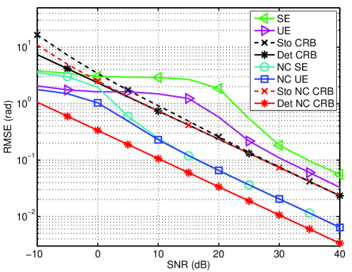
Figure 1: Analytical and empirical RMSEs versus SNR for the 12-element 2-D array ($R=2$) from Fig. 2, and $N=20$, $d=3$ correlated sources ($\rho=0.9$) at $\mu_{1}^{(1)}=0.25$, $\mu_{2}^{(1)}=0.25$, $\mu_{1}^{(2)}=0.5$, $\mu_{2}^{(2)}=0.5$, $\mu_{1}^{(3)}=0.75$, $\mu_{2}^{(3)}=0.75$ with rotation phases $\varphi_{1}=0$, $\varphi_{2}=\pi/4$, and $\varphi_{3}=\pi/2$.

\psfrag{Jxx}{\footnotesize{\color[rgb]{1,0,0} $\bm{J}_{1}^{(1)}$}}\psfrag{J12}{\footnotesize{\color[rgb]{0,1,0} $\bm{J}_{2}^{(1)}$}}\psfrag{J22}{\footnotesize{\color[rgb]{1,0,0} $\bm{J}_{1}^{(2)}$}}\psfrag{J21}{\footnotesize{\color[rgb]{0,1,0} $\bm{J}_{2}^{(2)}$}}\includegraphics[width=303.53267pt]{Figures/array_2d_shinv2}

Figure 2: 2-D shift invariance for the depicted centro-symmetric $4\times 3$ sampling grid, left: subarrays for the first (horizontal) dimension, right: subarrays for the second (vertical) dimension.

In Table I, we analyze the Det 1-D CRB and the Det 1-D NC CRB for a varying number of sources $d$ in case of a ULA with $M=4$, $N=20$, and $\mathrm{SNR}=10$ dB. The spatial frequencies $\mu_{i},~{}\forall i$ are distributed equally in the interval $[-2,2]$ and the rotation phases $\varphi_{i},~{}\forall i$ are drawn randomly. It can be seen that $d_{\rm max}=M-1$ for the CRB and $d_{\rm max}^{({\rm nc})}=2(M-1)$ for the NC CRB are the largest numbers of $d$ that lead to an invertible Fisher matrix, otherwise, the problem is ill-posed. Therefore, twice as many sources can be resolved from the strictly non-circular data model.

VI-B Analytical Results

In this subsection, we compare the analytical results “ana” in (43) and (46) to the empirical ones “emp” in (13) and Corollary 1 obtained by averaging over 1000 Monte-Carlo trials. We have $d=2$ sources that impinge on a ULA (1-D) with the powers $P_{1}=0.5$ and $P_{2}=1.5$. The symbols $\bm{S}_{0}$ are randomly drawn from a real-valued Gaussian distribution.

In Fig. 3, we display the RMSE of the Det 1-D NC CRB and the Det 1-D CRB for $d=2$ sources as a function of the number of sensors $M$, where the square root of the analytical expressions is taken. The source separation is $\Delta\mu=0.1~{}\mathrm{rad}$ with $\mu_{1}=0$ and $\mu_{2}=0.1$, however, the actual positions are irrelevant and have no impact on the performance. The remaining parameters are given by $N=10$, $\Delta\varphi=\pi/3$, $\delta=(M-1)/2$, i.e., the phase reference is located at the first sensor element, and $\sigma_{\mathrm{n}}^{2}=0.032$. Moreover, the correlation coefficient $\rho$ is set to $\rho=0.8$. It is evident that the analytical results agree well with the empirical estimation errors and that both CRBs perform similarly for large $M$.

Fig. 4 illustrates the asymptotic NC gain in (49) for $d=2$ sources as a function of $\Delta\mu$. The number of sensors is fixed to $M=15$ and we have $\rho=0$, $\Delta\varphi=\pi/2$ as well as $\delta=0$. For comparison purposes, we have also included the curves for the analytical NC gain of NC SE from [9] for this specific scenario. It can be seen that the NC gain expression becomes accurate for small $\Delta\mu$ and that it is largest when $\Delta\mu$ goes to zero. Furthermore, the NC gain of NC SE is close to the maximum achievable NC gain computed from the NC CRB.

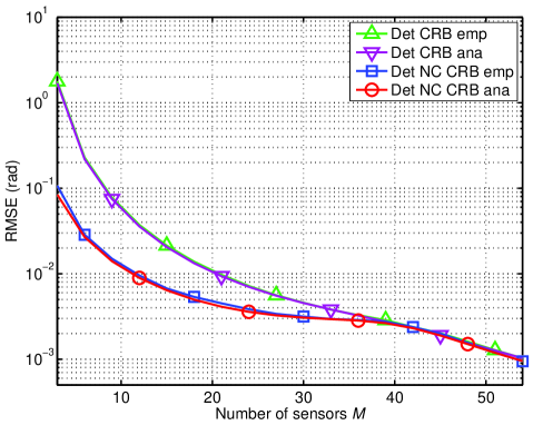
Figure 3: Analytical and empirical RMSEs versus the number of sensors $M$ for $d=2$ correlated sources with $N=10$, $\Delta\mu=0.1$ rad, $\rho=0.8$, $\Delta\varphi=\pi/3$, $\delta=(M-1)/2$, $P_{1}=1.5$, $P_{2}=0.5$, and $\sigma_{\mathrm{n}}^{2}=0.032$.

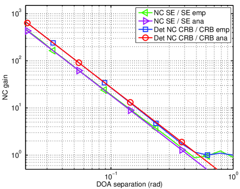
Figure 4: Analytical and empirical NC gain versus the source separation $\Delta\mu$ for $d=2$ uncorrelated sources with $M=15$, $N=10$, $\Delta\varphi=\pi/2$, $\delta=0$, $P_{1}=1.5$, $P_{2}=0.5$, and $\sigma_{\mathrm{n}}^{2}=0.032$.

TABLE I: RMSE for a varying number of sources with $M=4$

RMSE	$d=1$	$d=2$	$d=3$	$d=4$	$d=5$	$d=6$	$d=7$
CRB	$0.02$	$0.13$	$0.80$	$\infty$	$\infty$	$\infty$	$\infty$
NC CRB	$0.02$	$0.11$	$0.12$	$0.14$	$0.35$	$2.93$	$\infty$

VII Conclusion

In this paper, we have presented a closed-form expression of the deterministic $R$-D NC Cramér-Rao bound for multi-dimensional strictly non-circular (rectilinear) signals. This bound serves as a benchmark for the recently developed algorithms, e.g., $R$-D NC Standard ESPRIT and $R$-D NC Unitary ESPRIT, that exploit the NC structure of such strictly non-circular signals and thus outperform the traditional methods for arbitrary signals. Based on the resulting $R$-D NC CRB expression and assuming the $R$-D array to be separable and centro-symmetric, we have shown that in the special cases of equal phases and full coherence of the strictly non-circular signals as well as for a single strictly non-circular source, the deterministic $R$-D NC CRB reduces to the existing deterministic $R$-D CRB for arbitrary signals. This suggests that no NC gain can be achieved in these specific cases. Furthermore, we have simplified the derived NC CRB and the existing CRB for the special case of two closely-spaced strictly non-circular signals captured by a uniform linear array (ULA). With these simplified CRB expressions, we have then analytically computed the maximum achievable asymptotic NC gain for this scenario. The resulting expression only depends on the various physical parameters, e.g., the number of sensors, the signal correlation, etc. Additionally, we have analyzed the dependence of the NC gain on these parameters to find that the largest NC gain is obtained if the two sources are closely-spaced, incoherent, and have a non-vanishing phase discrimination.

Appendix A Proof of Theorem 1

For convenience, we start our derivation by vectorizing the $R$-D NC data model in (7) by using the property $\mathrm{vec}\{\bm{A}\bm{X}\bm{B}\}=(\bm{B}^{\rm T}\otimes\bm{A})\cdot\mathrm{vec}\{\bm{X}\}$ for arbitrary matrices $\bm{A}$, $\bm{B}$, and $\bm{X}$ of appropriate sizes. We obtain

$$\bm{x}=\mathop{{\rm vec}}\left\{\bm{X}\right\}=\left(\bm{I}_{N}\otimes\bm{A}\bm{\Psi}\right)\bm{s}_{0}+\bm{n}\in\mathbb{C}^{MN\times 1},$$ (52)

where $\bm{s}_{0}=\mathop{{\rm vec}}\left\{\bm{S}_{0}\right\}=[\bm{s}_{0}^{\rm T}(1),\ldots,\bm{s}_{0}^{\rm T}(N)]^{\rm T}\in{}^{Nd\times 1}$ with $\bm{s}_{0}(t),~{}t=1,\ldots,N$, being the $t$-th column of $\bm{S}_{0}$, and $\bm{n}=\mathop{{\rm vec}}\left\{\bm{N}\right\}\in\mathbb{C}^{MN\times 1}$. To suit the deterministic data assumption, the signal vector $\bm{s}_{0}$ is assumed to be deterministic and unknown to the receiver, while the sensor noise $\bm{n}$ is zero-mean circularly symmetric white complex Gaussian distributed, i.e., $\mathbb{E}\{\bm{n}\bm{n}^{\rm T}\}=\bm{0}$. Hence, the observations $\bm{x}$ satisfy the model

$$\bm{x}\sim\mathcal{CN}(\bm{\nu},\bm{\Sigma}),$$ (53)

where $\bm{\nu}=\left(\bm{I}_{N}\otimes\bm{A}\bm{\Psi}\right)\bm{s}_{0}$ and $\bm{\Sigma}=\sigma_{\mathrm{n}}^{2}\bm{I}_{MN}$ are the mean and the covariance of the array output vector $\bm{x}$.

Let us now define the real-valued vector of unknown parameters as

$$\bm{\xi}=\begin{bmatrix}\bm{\mu}^{\rm T}&\bm{s}_{0}^{\rm T}&\bm{\varphi}^{\rm T}&\sigma_{\mathrm{n}}^{2}\end{bmatrix}^{\rm T}\in{}^{[(R+N+1)d+1]\times 1}.$$ (54)

Here, $\bm{\mu}=[\bm{\mu}^{({1})^{\rm T}},\ldots,\bm{\mu}^{({R})^{\rm T}}]^{\rm T}\in{}^{Rd\times 1}$ is the principal parameter vector of interest and $\bm{s}_{0}\in{}^{Nd\times 1}$, $\bm{\varphi}\in{}^{d\times 1}$, and $\sigma_{\mathrm{n}}^{2}$ are the nuisance parameters. As the CRB matrix is usually computed by taking the inverse of the Fisher information matrix (FIM) $\bm{J}$, we first need to calculate $\bm{J}$. Due to (53), i.e., $\bm{x}$ is Gaussian distributed, the Slepian-Bangs formulation [15] of the FIM is still valid for the strictly non-circular data model in (52). Hence, the Slepian-Bangs formulation of $\bm{J}$ for the parameter vector $\bm{\xi}$ is given by [15]

$$\begin{aligned} \bm{J}_{p,q}&=\mathrm{Tr}\left\{\bm{\Sigma}^{-1}\frac{\partial\bm{\Sigma}}{\partial\bm{\xi}_{p}}\bm{\Sigma}^{-1}\frac{\partial\bm{\Sigma}}{\partial\bm{\xi}_{q}}\right\}\\ &\quad\quad\quad\quad\quad+2\cdot\mathrm{Re}\left\{\left(\frac{\partial\bm{\nu}}{\partial\bm{\xi}_{p}}\right)^{\rm H}\bm{\Sigma}^{-1}\frac{\partial\bm{\nu}}{\partial\bm{\xi}_{q}}\right\},\end{aligned}$$ (55)

$$\qquad\qquad\qquad~{}p,q=1,\ldots,(R+N+1)d+1.$$

Note that we are only interested in the CRB for $\bm{\mu}$, denoted as $\bm{C}^{({\rm nc})}$. Therefore, it is sufficient to compute the upper left block of $\bm{J}^{-1}$. In order to find $\bm{J}$ from (55), the partial derivatives of $\bm{\nu}$ with respect to the parameters of $\bm{\xi}$ can be calculated straightforwardly. We have

$$\frac{\partial\bm{\nu}}{\partial\bm{\mu}^{\rm T}} =\left(\bm{I}_{N}\otimes(\bm{D}(\bm{I}_{R}\otimes\bm{\Psi}))\right)\tilde{\bm{S}}^{({R})}_{0}\in\mathbb{C}^{MN\times Rd},$$ (56)

where $\bm{D}$ is given in (10) and $\tilde{\bm{S}}^{({R})}_{0}=[(\bm{I}_{R}\otimes\tilde{\bm{S}_{0}}(1)),\ldots,(\bm{I}_{R}\otimes\tilde{\bm{S}_{0}}(N))]^{\rm T}\in{}^{NRd\times Rd}$ with $\tilde{\bm{S}_{0}}(t)=\mathop{{\rm diag}}\left\{\bm{s}_{0}(t)\right\}\in{}^{d\times d}$. For the remaining parameters, we get

$$\frac{\partial\bm{\nu}}{\partial\bm{s}_{0}^{\rm T}} =\left(\bm{I}_{N}\otimes\bm{A}\bm{\Psi}\right)\in\mathbb{C}^{MN\times Nd},$$

$$\frac{\partial\bm{\nu}}{\partial\bm{\varphi}^{\rm T}} =\mathrm{j}\left(\bm{I}_{N}\otimes\bm{A}\bm{\Psi}\right)\tilde{\bm{S}}_{0}\in\mathbb{C}^{MN\times d},~{}~{}\frac{\partial\bm{\nu}}{\partial\sigma_{\mathrm{n}}^{2}}=\bm{0}\in{}^{MN\times 1},$$

where $\tilde{\bm{S}}_{0}=[\tilde{\bm{S}_{0}}(1),\ldots,\tilde{\bm{S}_{0}}(N)]^{\rm T}\in{}^{Nd\times d}$. Next, these results are combined to obtain

$$\frac{d\bm{\nu}}{d\bm{\xi}^{\rm T}} =\left[\begin{matrix}\left(\bm{I}_{N}\otimes(\bm{D}(\bm{I}_{R}\otimes\bm{\Psi}))\right)\tilde{\bm{S}}^{({R})}_{0}&\left(\bm{I}_{N}\otimes\bm{A}\bm{\Psi}\right),\end{matrix}\right.$$

$$\quad~{}\left.\begin{matrix}\mathrm{j}\left(\bm{I}_{N}\otimes\bm{A}\bm{\Psi}\right)\tilde{\bm{S}}_{0}&\bm{0}\end{matrix}\right]\in\mathbb{C}^{MN\times[(R+N+1)d+1]},$$ (57)

As for the derivative of $\bm{\Sigma}$ with respect to $\bm{\xi}$, the only non-zero term is

$$\frac{d\bm{\Sigma}}{d\sigma_{\mathrm{n}}^{2}}=\bm{I}_{MN},$$ (58)

such that

$$\frac{d\bm{\Sigma}}{d\bm{\xi}^{\rm T}}=\begin{bmatrix}\bm{0}&\bm{0}&\bm{0}&\bm{I}_{MN}\end{bmatrix}\in\mathbb{C}^{MN\times[(R+N+1)d+MN]}.$$ (59)

Inserting (57) and (59) into (55) and bearing in mind that we are interested in the $\bm{\mu}$-block of $\bm{J}$, only the second term of (55) is of concern. Therefore, we only consider the non-zero block $\tilde{\bm{J}}$ of $\bm{J}$, which is given by

$$\tilde{\bm{J}}=\begin{bmatrix}\bm{J}_{\bm{\mu},\bm{\mu}}&\bm{J}_{\bm{\mu},\bm{s}_{0}}&\bm{J}_{\bm{\mu},\bm{\varphi}}\\ \bm{J}_{\bm{s}_{0},\bm{\mu}}&\bm{J}_{\bm{s}_{0},\bm{s}_{0}}&\bm{J}_{\bm{s}_{0},\bm{\varphi}}\\ \bm{J}_{\bm{\varphi},\bm{\mu}}&\bm{J}_{\bm{\varphi},\bm{s}_{0}}&\bm{J}_{\bm{\varphi},\bm{\varphi}}\end{bmatrix}=\frac{2}{\sigma_{\mathrm{n}}^{2}}\cdot\mathrm{Re}\left\{\bm{G}^{\rm H}\bm{G}\right\},$$ (60)

where

$$\bm{G} =\left[\begin{matrix}\left(\bm{I}_{N}\otimes(\bm{D}(\bm{I}_{R}\otimes\bm{\Psi}))\right)\tilde{\bm{S}}^{({R})}_{0}&\left(\bm{I}_{N}\otimes\bm{A}\bm{\Psi}\right),\end{matrix}\right.$$

$$\quad\quad\quad\quad\quad\left.\begin{matrix}\mathrm{j}\left(\bm{I}_{N}\otimes\bm{A}\bm{\Psi}\right)\tilde{\bm{S}}_{0}\end{matrix}\right]\in\mathbb{C}^{MN\times(R+N+1)d}.$$ (61)

It is easy to see that $\tilde{\bm{J}}=\tilde{\bm{J}}^{\rm T}$. Consequently, only the block matrices on and above the diagonal of $\tilde{\bm{J}}$ need to be computed. For the block matrix $\bm{J}_{\bm{\mu},\bm{\mu}}$, we obtain

$$\bm{J}_{\bm{\mu},\bm{\mu}} =\frac{2}{\sigma_{\mathrm{n}}^{2}}\cdot\sum_{t=1}^{N}\mathop{{\rm Re}}\left\{(\bm{I}_{R}\otimes\tilde{\bm{S}}_{0}(t))(\bm{I}_{R}\otimes\bm{\Psi}^{*})\bm{D}^{\rm H}\right.$$

$$\left.\quad\quad\quad\quad\quad\quad\quad\quad\cdot\bm{D}(\bm{I}_{R}\otimes\bm{\Psi})(\bm{I}_{R}\otimes\tilde{\bm{S}}_{0}(t))\right\}$$ (62)

$$=\frac{2}{\sigma_{\mathrm{n}}^{2}}\cdot\mathrm{Re}\Bigg{\{}\left((\bm{I}_{R}\otimes\bm{\Psi}^{*})\bm{D}^{\rm H}\bm{D}(\bm{I}_{R}\otimes\bm{\Psi})\right)\Bigg{.}$$

$$\left.\quad\quad\quad\quad\quad\odot\sum_{t=1}^{N}(\bm{1}_{R}\otimes\bm{s}_{0}(t))(\bm{1}_{R}\otimes\bm{s}_{0}(t))^{\rm T}\right\}$$ (63)

$$=\frac{2}{\sigma_{\mathrm{n}}^{2}}\cdot\mathrm{Re}\Bigg{\{}\left((\bm{I}_{R}\otimes\bm{\Psi}^{*})\bm{D}^{\rm H}\bm{D}(\bm{I}_{R}\otimes\bm{\Psi})\right)\Bigg{.}$$

$$\left.\quad\quad\quad\quad\quad\quad\quad\odot\left(\bm{1}_{R\times R}\otimes\sum_{t=1}^{N}\bm{s}_{0}(t)\bm{s}^{\rm T}_{0}(t)\right)\right\}$$ (64)

$$=\frac{2N}{\sigma_{\mathrm{n}}^{2}}\cdot\mathrm{Re}\Bigg{\{}\left((\bm{I}_{R}\otimes\bm{\Psi}^{*})\bm{D}^{\rm H}\bm{D}(\bm{I}_{R}\otimes\bm{\Psi})\right)\Bigg{.}$$

$$\left.\quad\quad\quad\quad\quad\quad\quad\odot\left(\bm{1}_{R\times R}\otimes\frac{1}{N}\bm{S}_{0}\bm{S}_{0}^{\rm T}\right)\right\}$$ (65)

$$=\frac{2N}{\sigma_{\mathrm{n}}^{2}}\cdot\bm{G}_{2}\odot\hat{\bm{R}}^{({R})}_{S_{0}}\in{}^{Rd\times Rd},$$ (66)

where $\bm{G}_{2}$ is defined according to (20) and we have used the fact that $\mathop{{\rm diag}}\left\{\bm{a}\right\}\bm{C}\mathop{{\rm diag}}\left\{\bm{b}\right\}=\bm{C}\odot(\bm{a}\bm{b}^{\rm T})$ for arbitrary vectors $\bm{a}\in\mathbb{C}^{M},\bm{b}\in\mathbb{C}^{N}$, and a matrix $\bm{C}\in\mathbb{C}^{M\times N}$. In a similar manner, the other blocks of $\tilde{\bm{J}}$ can be computed. The results are given by

$$\bm{J}_{\bm{s}_{0},\bm{s}_{0}} =\frac{2}{\sigma_{\mathrm{n}}^{2}}\cdot\bm{I}_{N}\otimes\bm{G}_{0}\in{}^{Nd\times Nd}$$ (67)

$$\bm{J}_{\bm{\varphi},\bm{\varphi}} =\frac{2N}{\sigma_{\mathrm{n}}^{2}}\cdot\bm{G}_{0}\odot\hat{\bm{R}}_{S_{0}}\in{}^{d\times d}$$ (68)

$$\bm{J}_{\bm{\mu},\bm{s}_{0}} =\frac{2}{\sigma_{\mathrm{n}}^{2}}\cdot\tilde{\bm{S}}^{({R})^{\rm T}}_{0}\left(\bm{I}_{N}\otimes\bm{G}_{1}\right)\in{}^{Rd\times Nd}$$ (69)

$$\bm{J}_{\bm{s}_{0},\bm{\varphi}} =-\frac{2}{\sigma_{\mathrm{n}}^{2}}\cdot\left(\bm{I}_{N}\otimes\bm{H}_{0}\right)\tilde{\bm{S}_{0}}\in{}^{Nd\times d}$$ (70)

$$\bm{J}_{\bm{\mu},\bm{\varphi}} =-\frac{2N}{\sigma_{\mathrm{n}}^{2}}\cdot\bm{H}_{1}\odot(\bm{1}_{R}\otimes\bm{\hat{R}}_{S_{0}})\in{}^{Rd\times d},$$ (71)

where the matrices $\bm{G}_{n}$ and $\bm{H}_{n},~{}n=0,1,2$ are given in (16)-(19). Note that we have the symmetries $\bm{G}_{0}=\bm{G}_{0}^{\rm T}$, $\bm{G}_{2}=\bm{G}_{2}^{\rm T}$, and $\bm{H}_{0}=-\bm{H}_{0}^{\rm T}$.

In the next step, we need to extract the upper left block of $\tilde{\bm{J}}^{-1}$. To this end, we make use of the following lemma:

Lemma 2.

For matrices $\bm{{A}}\in\mathbb{C}^{p\times p}$, $\bm{{B}}\in\mathbb{C}^{p\times q}$, $\bm{{C}}\in\mathbb{C}^{p\times r}$, $\bm{{D}}\in\mathbb{C}^{q\times p}$, $\bm{{E}}\in\mathbb{C}^{q\times q}$, $\bm{{F}}\in\mathbb{C}^{q\times r}$, $\bm{{G}}\in\mathbb{C}^{r\times p}$, $\bm{{H}}\in\mathbb{C}^{r\times q}$, and $\bm{{J}}\in\mathbb{C}^{r\times r}$ the upper left $p\times p$ block of the matrix

$$\bm{{K}}=\begin{bmatrix}\bm{{A}}&\bm{{B}}&\bm{{C}}\\ \bm{{D}}&\bm{{E}}&\bm{{F}}\\ \bm{{G}}&\bm{{H}}&\bm{{J}}\end{bmatrix}^{-1}$$ (72)

is given by

$$\bm{{K}}_{1:p,1:p} =\Big{(}\bm{{A}}-\bm{{B}}\bm{{E}}^{-1}\bm{{D}}-\bm{{B}}\bm{{E}}^{-1}\bm{{F}}\bm{{S}}_{E}^{-1}\bm{{H}}\bm{{E}}^{-1}\bm{{D}}$$

$$+\bm{{B}}\bm{{E}}^{-1}\bm{{F}}\bm{{S}}_{E}^{-1}\cdot\bm{{G}}+\bm{{C}}\bm{{J}}^{-1}\bm{{H}}\bm{{E}}^{-1}\bm{{D}}$$

$$+\bm{{C}}\bm{{J}}^{-1}\bm{{H}}\bm{{E}}^{-1}\cdot\bm{{F}}\bm{{S}}_{E}^{-1}\bm{{H}}\bm{{E}}^{-1}\bm{{D}}-\bm{{C}}\bm{{S}}_{E}^{-1}\bm{{G}}\Big{)}^{-1},$$

where $\bm{{S}}_{E}=\bm{{J}}-\bm{{H}}\bm{{E}}^{-1}\bm{{F}}$.

Proof:

The proof of Lemma 2 can easily be constructed by applying the inversion formula for a $2\times 2$ block-partitioned matrix [20] to the $3\times 3$ block matrix in (72) twice. ∎

Applying Lemma 2 to compute the upper left block of $\tilde{\bm{J}}^{-1}$, it is straightforward to obtain the expression in (15), where we have

$$\bm{{S}}_{E} =\frac{2N}{\sigma_{\mathrm{n}}^{2}}\cdot\left(\bm{{G}}_{0}-\bm{{H}}_{0}^{\rm T}\bm{{G}}_{0}^{-1}\bm{{H}}_{0}\right)\odot\hat{\bm{R}}^{({R})}_{S_{0}}$$

$$\bm{{B}}\bm{{E}}^{-1}\bm{{D}} =\frac{2N}{\sigma_{\mathrm{n}}^{2}}\cdot\left(\bm{{G}}_{1}\bm{{G}}_{0}^{-1}\bm{{G}}_{1}^{\rm T}\right)\odot\hat{\bm{R}}^{({R})}_{S_{0}}$$

$$\bm{{B}}\bm{{E}}^{-1}\bm{{F}} =-\frac{2N}{\sigma_{\mathrm{n}}^{2}}\cdot\left(\bm{{G}}_{1}\bm{{G}}_{0}^{-1}\bm{{H}}_{0}\right)\odot\hat{\bm{R}}^{({R})}_{S_{0}}$$

$$\bm{{H}}\bm{{E}}^{-1}\bm{{D}} =-\frac{2N}{\sigma_{\mathrm{n}}^{2}}\cdot\left(\bm{{H}}_{0}^{\rm T}\bm{{G}}_{0}^{-1}\bm{{G}}_{1}^{\rm T}\right)\odot\hat{\bm{R}}^{({R})}_{S_{0}}$$

$$\bm{{H}}\bm{{E}}^{-1}\bm{{F}} =\frac{2N}{\sigma_{\mathrm{n}}^{2}}\cdot\left(\bm{{H}}_{0}^{\rm T}\bm{{G}}_{0}^{-1}\bm{{H}}_{0}\right)\odot\hat{\bm{R}}^{({R})}_{S_{0}}.$$

This concludes the proof. ∎

Appendix B

In this section, we prove that for $\delta^{({r})}=0~{}\forall\;r$ and subsequently $\bm{A}=\bar{\bm{A}}$, the matrices $\bm{A}^{\rm H}\bm{A}\in{}^{d\times d}$, $\bm{D}^{\rm H}\bm{A}\in{}^{Rd\times d}$, and $\bm{D}^{\rm H}\bm{D}\in{}^{Rd\times Rd}$ are real-valued. To this end, we make use of the following lemma:

Lemma 3.

For two arbitrary non-singular left $\bm{\Pi}$-real matrices $\bm{X}\in\mathbb{C}^{M\times N}$ and $\bm{Y}\in\mathbb{C}^{M\times N}$ satisfying $\bm{\Pi}\bm{X}^{*}=\bm{X}$ and $\bm{\Pi}\bm{Y}^{*}=\bm{Y}$, respectively, the following identity holds:

$$\bm{Y}^{\rm H}\bm{X} =(\bm{\Pi}\bm{Y}^{*})^{\rm H}\bm{\Pi}\bm{X}^{*}=\bm{Y}^{\rm T}\bm{\Pi}\bm{\Pi}\bm{X}^{*}$$

$$=(\bm{Y}^{\rm H}\bm{X})^{*}\in{}^{N\times N}.$$ (73)

Therefore, to prove that the aforementioned matrices are real-valued, we simply show that the matrices $\bm{A}$ and $\bm{D}$ are left $\bm{\Pi}$-real. It is straightforward to see that due to $\delta^{({r})}=0~{}\forall\;r$, this is the case for $\bm{A}$ (cf. Equation (24)). As for the matrix $\bm{D}$, we utilize the linearity of the differentiation operator and obtain

$$\bm{\Pi}\bm{D}^{*} =\bm{\Pi}\left(\frac{\partial\bm{A}}{\partial\bm{\mu}}\right)^{*}=\frac{\partial\bm{\Pi}\bm{A}^{*}}{\partial\bm{\mu}}=\frac{\partial\bm{A}}{\partial\bm{\mu}}=\bm{D},$$ (74)

which also renders $\bm{D}$ left $\bm{\Pi}$-real and concludes the proof. ∎

Appendix C Proof of Theorem 2

Evaluating the $R$-D NC CRB in (15) for the special case $d=1$, the array steering matrix $\bm{A}$ reduces to $\bm{a}(\bm{\mu})$, $\bm{D}=[\bm{d}^{(1)},\ldots,\bm{d}^{(R)}]\in\mathbb{C}^{M\times R}$, $\bm{\Psi}={{\rm e}}^{\mathrm{j}\varphi}$, and $\hat{\bm{R}}_{S_{0}}=\bm{s}_{0}^{\rm T}\bm{s}_{0}/N=\hat{P}$, where $\bm{s}_{0}\in{}^{N\times 1}$. Moreover, we choose $\delta^{({r})}=0~{}\forall\;r$ for simplicity. Then, dropping the dependence of $\bm{a}$ on $\bm{\mu}$ and utilizing the definitions in (3) and (11), respectively, we have

$$\bm{a}^{\rm H}\bm{a} =\prod_{r=1}^{R}\bm{a}^{({r})^{\rm H}}\bm{a}^{({r})}=\prod_{r=1}^{R}M_{r}=M,$$ (75)

$$\bm{d}^{({r})^{\rm H}}\bm{a} =\prod_{\begin{subarray}{c}p=1\\ p\neq r\end{subarray}}^{R}\bm{a}^{({p})^{\rm H}}\bm{a}^{({p})}\cdot\tilde{\bm{d}}^{({r})^{\rm H}}\bm{a}^{({r})}$$

$$=\prod_{\begin{subarray}{c}p=1\\ p\neq r\end{subarray}}^{R}\bm{a}^{({p})^{\rm H}}\bm{a}^{({p})}\cdot\left(-\mathrm{j}\sum_{m_{r}=1}^{M_{r}}k_{m_{r}}\right)=0~{}~{}\forall\;r,$$ (76)

$$\bm{d}^{({r})^{\rm H}}\bm{d}^{({r})} =\prod_{\begin{subarray}{c}p=1\\ p\neq r\end{subarray}}^{R}\bm{a}^{({p})^{\rm H}}\bm{a}^{({p})}\cdot\tilde{\bm{d}}^{({r})^{\rm H}}\tilde{\bm{d}}^{({r})}$$

$$=\prod_{\begin{subarray}{c}p=1\\ p\neq r\end{subarray}}^{R}\bm{a}^{({p})^{\rm H}}\bm{a}^{({p})}\cdot\left(\sum_{m_{r}=1}^{M_{r}}k_{m_{r}}^{2}\right)$$

$$=\frac{M}{M_{r}}\sum_{m_{r}=1}^{M_{r}}k_{m_{r}}^{2}=\Gamma^{({r})}~{}~{}\forall\;r.$$ (77)

Using the results in (75)-(77), the matrices $\bm{G}_{n}$ and $\bm{H}_{n},~{}n=0,1,2,$ simplify to

$$\bm{G}_{0} =M,\quad\quad\bm{G}_{1}=\bm{H}_{0}=\bm{H}_{1}=0,$$ (78)

$$\bm{G}_{2} =\bm{D}^{\rm H}\bm{D}=\mathop{{\rm diag}}\left\{\left[\Gamma^{(1)},\ldots,\Gamma^{({R})}\right]\right\},$$ (79)

where in $\bm{G}_{2}$, the terms $\bm{d}^{(r_{1})^{\rm H}}\bm{d}^{(r_{2})}$ for $r_{1}\neq r_{2}$ evaluate to zero due to (76). Inserting these expressions into (15), the remaining part of the $R$-D NC CRB matrix is given by

$$\bm{C}^{({\rm nc})} =\frac{\sigma_{\mathrm{n}}^{2}}{2N\hat{P}}\cdot\left\{\mathop{{\rm diag}}\left\{\left[\Gamma^{(1)},\ldots,\Gamma^{({R})}\right]\right\}\right\}^{-1}$$ (80)

$$=\mathop{{\rm diag}}\left\{\left[{C^{({\rm nc})}}^{(1)},\ldots,{C^{({\rm nc})}}^{(R)}\right]\right\}\in{}^{R\times R},$$ (81)

where

$${C^{({\rm nc})}}^{({r})}=\frac{\sigma_{\mathrm{n}}^{2}}{2N\hat{P}}\cdot\frac{M_{r}}{M}\cdot\frac{1}{\sum_{m_{r}=1}^{M_{r}}k_{m_{r}}^{2}}~{}\forall\;r,$$ (82)

which is the desired result. ∎

Appendix D Proof of Theorem 3

Based on the model in (28) after inserting (41), we start the proof by assuming without loss of generality that the phase reference is at the array centroid, i.e., $\bm{\Delta}=\bm{I}_{d}$ such that $\bm{A}=\bar{\bm{A}}$ and $\bm{\Phi}=\bm{\Psi}$. Using the results from Appendix B, we can write the real-valued matrices $\bm{A}^{\rm H}\bm{A}$, $\bm{D}^{\rm H}\bm{A}$, and $\bm{D}^{\rm H}\bm{D}$ as

$$\bm{A}^{\rm H}\bm{A}=\begin{bmatrix}M&\alpha\\ \alpha&M\end{bmatrix}\!,~{}\bm{D}^{\rm H}\bm{A}=\begin{bmatrix}0&\beta\\ -\beta&0\end{bmatrix},~{}\bm{D}^{\rm H}\bm{D}=\begin{bmatrix}\Gamma&\gamma\\ \gamma&\Gamma\end{bmatrix},$$

where we have defined $\alpha=\bm{a}_{1}^{\rm H}\bm{a}_{2}=\bm{a}_{2}^{\rm H}\bm{a}_{1}$, $\beta=\bm{d}_{1}^{\rm H}\bm{a}_{2}=-\bm{d}_{2}^{\rm H}\bm{a}_{1}$, and $\gamma=\bm{d}_{1}^{\rm H}\bm{d}_{2}=\bm{d}_{2}^{\rm H}\bm{d}_{1}$. Then, the matrices $\bm{G}_{0}$ and $\bm{H}_{0}$ can be written as

$$\bm{G}_{0} =\mathop{{\rm Re}}\left\{\bm{\Psi}^{*}\bm{A}^{\rm H}\bm{A}\bm{\Psi}\right\}=\begin{bmatrix}M&\alpha\cdot\cos(\Delta\varphi)\\ \alpha\cdot\cos(\Delta\varphi)&M\end{bmatrix}$$

$$\bm{H}_{0} =\mathop{{\rm Im}}\left\{\bm{\Psi}^{*}\bm{A}^{\rm H}\bm{A}\bm{\Psi}\right\}=\begin{bmatrix}0&\alpha\cdot\sin(\Delta\varphi)\\ -\alpha\cdot\sin(\Delta\varphi)&0\end{bmatrix}.$$

The matrices $\bm{G}_{1}$, $\bm{H}_{1}$, and $\bm{G}_{2}$ can be expressed in a similar manner. In order to obtain an expression of the 1-D NC CRB that only depends on the physical parameters, e.g, $M$, $\rho$, $\Delta\varphi$, etc., we approximate the scalars $\alpha$, $\beta$, and $\gamma$ using a Taylor series expansion for small source separations $\Delta\mu=|\mu_{2}-\mu_{1}|$. Hence, these approximations become accurate for a small $\Delta\mu$. Therefore, for $\alpha$, we have

$$\alpha =\sum_{m=-\frac{(M-1)}{2}}^{\frac{(M-1)}{2}}{\rm e}^{\mathrm{j}m\Delta\mu}\approx M+\mathrm{j}\Delta\mu\cdot\sum_{m=-\frac{(M-1)}{2}}^{\frac{(M-1)}{2}}m$$

$$-\frac{\Delta\mu^{2}}{2}\cdot\sum_{m=-\frac{(M-1)}{2}}^{\frac{(M-1)}{2}}m^{2}-~{}\cdots$$

$$\approx M-\frac{M}{24}\Delta\mu^{2}(M^{2}-1)+\mathcal{O}(\Delta\mu^{4}).$$

Note that the terms containing odd powers of $m$ evaluate to zero. Similarly, in case of a small $\Delta\mu$, we get for $\beta$ and $\gamma$ the expressions

$$\beta =-\mathrm{j}\cdot\sum_{m=-\frac{(M-1)}{2}}^{\frac{(M-1)}{2}}m\cdot{\rm e}^{\mathrm{j}m\Delta\mu}$$

$$\approx-\mathrm{j}\cdot\sum_{m=-\frac{(M-1)}{2}}^{\frac{(M-1)}{2}}m\cdot\left(1+\mathrm{j}m\Delta\mu-\frac{\Delta\mu^{2}}{2}m^{2}-~{}\cdots\right)$$

$$\approx\frac{M}{12}\Delta\mu(M^{2}-1)-\frac{M}{1440}\Delta\mu^{3}(3M^{4}-10M^{2}+7)+\mathcal{O}(\Delta\mu^{5}),$$

$$\gamma =\sum_{m=-\frac{(M-1)}{2}}^{\frac{(M-1)}{2}}m^{2}\cdot{\rm e}^{\mathrm{j}m\Delta\mu}$$

$$\approx-\mathrm{j}\cdot\sum_{m=-\frac{(M-1)}{2}}^{\frac{(M-1)}{2}}m^{2}\cdot(1+\mathrm{j}m\Delta\mu-\frac{\Delta\mu^{2}}{2}m^{2}-~{}\cdots)$$

$$\approx\frac{M}{12}(M^{2}-1)-\frac{M}{480}\Delta\mu^{2}(3M^{4}-10M^{2}+7)+\mathcal{O}(\Delta\mu^{4}).$$

Finally, with the sample covariance matrix

$$\hat{\bm{R}}_{S_{0}}=\begin{bmatrix}\hat{P}_{1}&\hat{\rho}\sqrt{\hat{P}_{1}\hat{P}_{2}}\\ \hat{\rho}\sqrt{\hat{P}_{1}\hat{P}_{2}}&\hat{P}_{2}\end{bmatrix}$$ (83)

and the help of the Taylor approximation terms above, we can evaluate the 1-D NC CRB expression in Corollary 1 for two closely-spaced strictly non-circular sources. Due to the cancellation of relevant terms when using only approximation terms of lower order, we also need to consider higher-order Taylor approximation terms for $\alpha$, $\beta$, and $\gamma$. After some tedious calculations, we obtain

$$\mathop{{\rm Tr}}\left\{\bm{C}^{({\rm nc})}\right\}=\frac{\sigma_{\mathrm{n}}^{2}}{2N}\cdot z\cdot\frac{\hat{P}_{1}+\hat{P}_{2}}{\hat{P}_{1}\hat{P}_{2}},$$ (84)

where

$$z=\frac{x_{0}+x_{1}\Delta\mu^{2}+x_{2}\Delta\mu^{4}+\cdots}{y_{1}\Delta\mu^{2}+y_{2}\Delta\mu^{4}+y_{3}\Delta\mu^{6}+\cdots}.$$ (85)

It is apparent that the first term in the numerator and the first two terms in the denominator of (84) are dominant. Neglecting the non-relevant higher-order terms in the numerator and denominator of (84) and applying some algebraic manipulations, an expression in the form of (43) can be deduced. Finally, to make the result more general, we consider an arbitrary phase reference and substitute $\Delta\varphi$ by $\Delta\phi$ to obtain (43). This concludes the proof. ∎

Appendix E Proof of Theorem 4

The proof of Theorem 4 follows the same steps as the proof in Appendix D. Under the same assumptions, we compute the matrices $\bm{A}^{\rm H}\bm{A}$, $\bm{D}^{\rm H}\bm{A}$, and $\bm{D}^{\rm H}\bm{D}$ in the same way. The difference is, however, that we evaluate the 1-D CRB expression given in (8). Using the same Taylor series approximations as before, we obtain a similar expression as (84). Finally, neglecting the non-dominant terms in the numerator and the denominator, and substituting $\Delta\phi$ for $\Delta\varphi$, we arrive at the expression in (46) to prove this theorem. ∎

References

• [1] H. Abeida and J. P. Delmas, “MUSIC-like estimation of direction of arrival for noncircular sources,” IEEE Transactions on Signal Processing, vol. 54, no. 7, pp. 2678–2690, July 2006.
• [2] P. Chargé, Y. Wang, and J. Saillard, “A non-circular sources direction finding method using polynomial rooting,” Signal Processing, vol. 81, no. 8, pp. 1765–1770, Aug. 2001.
• [3] A. Zoubir, P. Chargé, and Y. Wang, “Non circular sources localization with ESPRIT,” in Proc. European Conference on Wireless Technology (ECWT), Munich, Germany, Oct. 2003.
• [4] M. Haardt and F. Roemer, “Enhancements of unitary ESPRIT for non-circular sources,” in Proc. IEEE Int. Conf. on Acoust., Speech, and Signal Processing (ICASSP), Montreal, Canada, May 2004.
• [5] J. Steinwandt, F. Roemer, M. Haardt, and G. Del Galdo, “R-dimensional ESPRIT-type algorithms for strictly second-order non-circular sources and their performance analysis,” IEEE Transactions on Signal Processing, vol. 62, no. 18, pp. 4824–4838, Sept. 2014.
• [6] P. J. Schreier and L. L. Scharf, Statistical Signal Processing of Complex-Valued Data: The Theory of Improper and Noncircular Signals, Cambridge University Press, 2010.
• [7] H. Krim and M. Viberg, “Two decades of array signal processing research: parametric approach,” IEEE Signal Processing Magazine, vol. 13, no. 4, pp. 67–94, July 1996.
• [8] F. Roemer, M. Haardt, and G. Del Galdo, “Analytical performance assessment of multi-dimensional matrix- and tensor-based ESPRIT-type algorithms,” IEEE Transactions on Signal Processing, vol. 62, no. 10, pp. 2611–2625, May 2014.
• [9] J. Steinwandt, F. Roemer, and M. Haardt, “Analytical ESPRIT-based performance study: What can we gain from non-circular sources?,” in Proc. 8th IEEE Sensor Array and Multichannel Signal Processing Workshop (SAM), A Coruña, Spain, June 2014.
• [10] P. Stoica and A. Nehorai, “MUSIC, maximum likelihood, and Cramer-Rao bound,” IEEE Transactions on Acoustics, Speech and Signal Processing, vol. 37, no. 5, pp. 720–741, May 1989.
• [11] P. Stoica, A. G. Larsson, and A. B. Gershman, “The stochastic CRB for array processing: A textbook derivation,” IEEE Signal Processing Letters, vol. 8, no. 5, pp. 148–150, May 2001.
• [12] J. P. Delmas and H. Abeida, “Stochastic Cramer-Rao bound for noncircular signals with application to DOA estimation,” IEEE Transactions on Signal Processing, vol. 52, no. 11, pp. 3192–3199, Nov. 2004.
• [13] H. Abeida and J. P. Delmas, “Gaussian Cramer-Rao bound for direction estimation of noncircular signals in unknown noise fields,” IEEE Transactions on Signal Processing, vol. 53, no. 12, pp. 4610–4618, Dec. 2005.
• [14] J. P. Delmas and H. Abeida, “Cramer-Rao bounds of DOA estimates for BPSK and QPSK modulated signals,” IEEE Transactions on Signal Processing, vol. 54, no. 1, pp. 117–126, Jan. 2006.
• [15] P. Stoica and R. L. Moses, Spectral Analysis of Signals, Upper Saddle River, NJ: Prentice-Hall, 2005.
• [16] F. Roemer and M. Haardt, “Deterministic Cramér-Rao bounds for strict sense non-circular sources,” in Proc. ITG/IEEE Workshop on Smart Antennas (WSA), Vienna, Austria, Feb. 2007.
• [17] M. Haardt and J. A. Nossek, “Simultaneous Schur decomposition of several non-symmetric matrices to achieve automatic pairing in multidimensional harmonic retrieval problems,” IEEE Transactions on Signal Processing, vol. 46, no. 1, pp. 161–169, Jan. 1998.
• [18] M. Haardt and J. A. Nossek, “Unitary ESPRIT: How to obtain increased estimation accuracy with a reduced computational burden,” IEEE Transactions on Signal Processing, vol. 43, no. 5, pp. 1232–1242, May 1995.
• [19] F. Roemer and M. Haardt, “A framework for the analytical performance assessment of matrix and tensor-based ESPRIT-type algorithms,” pre-print, Sept. 2012, arXiv:1209.3253.
• [20] H. Lütkepohl, Handbook of Matrices, John Wiley and Sons, 1996.