NonLocal Systems of Balance Laws
in Several Space Dimensions
with Applications to Laser Technology

Abstract

For a class of systems of nonlinear and nonlocal balance laws in several space dimensions, we prove the local in time existence of solutions and their continuous dependence on the initial datum. The choice of this class is motivated by a new model devoted to the description of a metal plate being cut by a laser beam. Using realistic parameters, solutions to this model obtained through numerical integrations meet qualitative properties of real cuts. Moreover, the class of equations considered comprises a model describing the dynamics of solid particles along a conveyor belt.

Keywords: Nonlocal Balance Laws; Laser Cutting; Conveyor Belt Dynamics

2010 MSC: 35L65

1 Introduction

We are concerned with a system of $n$ balance laws in several space dimensions of the type

$$\left\{\begin{array}[]{l}\partial_{t}u_{i}+\mathop{\rm{div}}\nolimits_{x}\varphi_{i}(t,x,u_{i},\vartheta*u)=\Phi_{i}(t,x,u_{i},\vartheta*u)\\ u_{i}(0,x)=\bar{u}_{i}(x)\end{array}\right.\qquad i=1,\ldots,n\,.$$ (1.1)

Here, $t\in\left[0,+\infty\right[$ is time, $x\in{\mathbb{R}}^{N}$ is the space coordinate and $u\equiv(u_{1},\ldots,u_{n})$, with $u_{i}=u_{i}(t,x)$, is the unknown. The function $\vartheta$ is a smooth function defined in ${\mathbb{R}}^{N}$ attaining as values $m\times n$ matrices, so that

$$\vartheta\in\mathbf{C_{c}^{2}}({\mathbb{R}}^{N};{\mathbb{R}}^{m\times n})\,,\qquad\left(\vartheta*u(t)\right)(x)=\int_{{\mathbb{R}}^{N}}\vartheta(x-\xi)\;u(t,\xi)\mathinner{\mathrm{d}{\xi}}\,,\qquad\left(\vartheta*u(t)\right)(x)\in{\mathbb{R}}^{m}\,.$$

The flow $\varphi\equiv(\varphi_{1},\ldots,\varphi_{n})$, with $\varphi_{i}(t,x,u_{i},A)\in{\mathbb{R}}^{N}$, and the source $\Phi\equiv(\Phi_{1},\ldots,\Phi_{n})$, with $\Phi_{i}(t,x,u_{i},A)\in{\mathbb{R}}$, have the peculiar property that the equations are coupled only through the nonlocal convolution term $\vartheta*u$.

The driving example for our considering the class (1.1) is a new model for the cutting of metal plates by means of a laser beam, presented in Section 3. A sort of pattern formation phenomenon, typical of various nonlocal equations [7], accounts for the formation of the well known ripples whose insurgence deeply affects the quality of the cuts. In fact, two type of lasers are mainly used in the cutting of metals: $CO_{2}$ lasers and fiber lasers. The former ones are more powerful and more precise, but also more expensive. Recent technological improvements are apparently going to allow also to the cheaper devices of the latter type to cut thick plates, nowadays treated typically with $CO_{2}$ lasers. Unfortunately, a typical drawback of fiber lasers is that along the cut ripples are generated, see [26, 28, 33]. The modeling of these ripples often relies on the introduction of imperfections in the metal or of inaccuracies in the laser management, see also [25, 27]. Here, using realistic numeric parameters, we obtain the formation of a geometry similar to the ripples observed in industrial cuts. We remark that in the present construction neither the initial data nor the parameters in the equations contain any oscillating term.

Furthermore, in Section 4, we slightly extend the model introduced in [12] to describe the dynamics of bolts along a conveyor belt. The resulting equations fit in the present framework and is proved to be well posed.

Besides, we also note that several crowd dynamics models considered in the literature fit into (1.1), e.g. [7, 9, 11, 18].

The particular structure of (1.1) allows to prove its well posedness. Indeed, for small times, system (1.1) admits a unique solution $u=u(t,x)$. Moreover, $u$ is proved to be a continuous function of time with respect to the $\mathbf{L^{1}}$ topology and an $\mathbf{L^{1}}$–Lipschitz continuous function of the initial datum $\bar{u}$. In all this, the particular coupling among the equations in (1.1) plays a key role. At present, the well posedness of general systems of balance laws in several space dimensions is a formidable open problem. In the present work, the functional setting is provided by $\mathbf{L^{1}}\cap\mathbf{L^{\infty}}\cap\mathbf{BV}$, as usual in the framework of nonlocal conservation laws. The existence result is obtained through a careful use of the general estimates [10, 21]. They provide the necessary analytic tool to apply Banach Contraction Theorem.

A preliminary result related to Theorem 2.2 below is presented for instance in [1], see also [3]. There, the existence of solution to (1.1) in the case $\Phi\equiv 0$ is obtained proving the convergence (up to a subsequence) of a Lax–Friedrichs type approximate solutions. Note however that differently from the present situation, in the case considered in [1], positive initial data yield positive solutions so that the $\mathbf{L^{1}}$ norm is conserved.

We remark that most of the results related to nonlocal balance laws are currently devoted to conservation laws, i.e., to equations that lack any source term. Here, we allow for the presence of source terms that can be nonlinear in both the unknown variable $u$ and the convolution term $\vartheta*u$. The unavoidable cost of this extension is a local in time existence result, as shown by an example in Section 2.

Nonlocal conservation and balance laws are currently widely considered in various modeling frameworks. Besides those of crowd dynamics, laser cutting and conveyor belt dynamics considered above, we recall for instance granular materials, see [2], and vehicular traffic, see [4]. For a different approach, based on measure valued balance laws, we refer to [24].

The paper is organized as follows: the next section is devoted to the analytic results. Section 3 presents the laser cutting model, its well posedness and some qualitative properties with the help of numerical integrations. Conveyor belts dynamics is the subject of Section 4. All analytic proofs are postponed to the last Section 5.

2 Analytic Results

Throughout, we denote by $\mathop{\rm{grad}}\nolimits_{x}f$, respectively $\mathop{\rm{div}}\nolimits_{x}f$, the gradient, respectively the divergence, of $f$ with respect to the $x$ variable, with $x\in{\mathbb{R}}^{N}$. All norms in function spaces are denoted with a subscript indicating the space, as for instance in ${\left\|u(t)\right\|}_{\mathbf{L^{1}}({\mathbb{R}}^{N};{\mathbb{R}}^{n})}$. When no space is indicated, the norm is the usual Euclidean norm in ${\mathbb{R}}^{k}$, for a suitable $k$, as for instance in ${\left\|u(t,x)\right\|}$. Throughout, we fix the non trivial time interval $\widehat{I}=[0,\widehat{T}]$. For any $U>0$, we also denote $\mathcal{U}_{U}=[-U,\,U]$.

Our starting point is the definition of solution to (1.1), which extends [1, Definition 2.1] to the case of balance laws.

Definition 2.1.

Fix a positive $T$. Let $\bar{u}\in\mathbf{L^{\infty}}({\mathbb{R}}^{N},{\mathbb{R}}^{n})$. A map $u:[0,T]\rightarrow\mathbf{L^{\infty}}({\mathbb{R}}^{N},{\mathbb{R}}^{n})$ is a solution on $[0,T]$ to (1.1) with initial datum $\bar{u}$ if, for $i=1,\ldots,n$, setting for all $w\in{\mathbb{R}}$

$$\widetilde{\varphi_{i}}(t,x,w)=\varphi_{i}\left(t,x,w,(\vartheta*u)(t,x)\right)\qquad\mbox{ and }\qquad\widetilde{\Phi}_{i}(t,x,w)=\Phi_{i}\left(t,x,w,(\vartheta*u)(t,x)\right)$$

the map $u$ is a Kružkov solution to the system

$$\left\{\begin{array}[]{l}\partial_{t}u_{i}+\mathop{\rm{div}}\nolimits_{x}\widetilde{\varphi}_{i}(t,x,u_{i})=\widetilde{\Phi}_{i}(t,x,u_{i})\\ u_{i}(0,x)=\bar{u}_{i}(x)\end{array}\right.\qquad i=1,\ldots,n\,.$$ (2.1)

Above, for the definition of Kružkov solution we refer to the original [20, Definition 1].

We are now ready to state the main result of the present paper.

Theorem 2.2.

Assume that there exists a function $\lambda\in(\mathbf{C^{0}}\cap\mathbf{L^{1}})(\widehat{I}\times{\mathbb{R}}^{N}\times{\mathbb{R}}^{+};{\mathbb{R}}^{+})$ such that:

($\boldsymbol{\varphi}$)

For any $U>0$, $\varphi\in(\mathbf{C^{2}}\cap\mathbf{W^{2,\infty}})(\widehat{I}\times{\mathbb{R}}^{N}\times\mathcal{U}_{U}\times\mathcal{U}_{U}^{m};{\mathbb{R}}^{n\times N})$ and for all $t\in\widehat{I}$, $x\in{\mathbb{R}}^{N}$, $u\in\mathcal{U}_{U}$, $A\in\mathcal{U}_{U}^{m}$

$$\max\left\{\begin{array}[]{ll}{\left\|\mathop{\rm{grad}}\nolimits_{x}\varphi(t,x,u,A)\right\|}\,,&{\left\|\mathop{\rm{div}}\nolimits_{x}\varphi(t,x,u,A)\right\|}\,,\\[3.0pt] {\left\|\mathop{\rm{grad}}\nolimits_{x}\mathop{\rm{div}}\nolimits_{x}\varphi(t,x,u,A)\right\|}\,,&{\left\|\mathop{\rm{grad}}\nolimits_{x}\mathop{\rm{grad}}\nolimits_{A}\varphi(t,x,u,A)\right\|}\,,\\[3.0pt] {\left\|\mathop{\rm{grad}}\nolimits_{A}\varphi(t,x,u,A)\right\|}\,,&{\left\|\mathop{\rm{grad}}\nolimits_{A}^{2}\varphi(t,x,u,A)\right\|}\end{array}\right\}\leq\lambda(t,x,U)\,.$$

($\boldsymbol{\Phi}$)

For any $U>0$, $\Phi\in(\mathbf{C^{1}}\cap\mathbf{W^{1,\infty}})(\widehat{I}\times{\mathbb{R}}^{N}\times\mathcal{U}_{U}\times\mathcal{U}_{U}^{m};{\mathbb{R}}^{n})$ and for all $t\in\widehat{I}$, $x\in{\mathbb{R}}^{N}$, $u\in\mathcal{U}_{U}$, $A\in\mathcal{U}_{U}^{m}$

$$\max\left\{{\left\|\Phi(t,x,u,A)\right\|}\,,\;{\left\|\mathop{\rm{grad}}\nolimits_{x}\Phi(t,x,u,A)\right\|}\right\}\leq\lambda(t,x,U)\,.$$

($\boldsymbol{\vartheta}$)

$\vartheta\in\mathbf{C_{c}^{2}}({\mathbb{R}}^{N};{\mathbb{R}}^{m\times n})$.

Then, for any positive $\bar{\mathcal{C}}$ there exists a positive $T_{*}\in I$ and positive $\mathcal{L}$, $\mathcal{C}$ such that for any datum

$$\bar{u}\in(\mathbf{L^{1}}\cap\mathbf{L^{\infty}}\cap\mathbf{BV})({\mathbb{R}}^{N};{\mathbb{R}}^{n})\mbox{ with }{\left\|\bar{u}_{i}\right\|}_{\mathbf{L^{1}}({\mathbb{R}}^{N};{\mathbb{R}}^{n})}\leq\bar{\mathcal{C}},\;{\left\|\bar{u}_{i}\right\|}_{\mathbf{L^{\infty}}({\mathbb{R}}^{N};{\mathbb{R}}^{n})}\leq\bar{\mathcal{C}}\mbox{ and }\mathop{\mathrm{missing}}{TV}(\bar{u}_{i})\leq\bar{\mathcal{C}},$$ (2.2)

problem (1.1) admits a unique solution

$$u\in\mathbf{C^{0}}\left([0,T_{*}];\mathbf{L^{1}}({\mathbb{R}}^{N};{\mathbb{R}}^{n})\right)$$

in the sense of Definition 2.1, satisfying the bounds

$${\left\|u(t)\right\|}_{\mathbf{L^{1}}({\mathbb{R}}^{N};{\mathbb{R}}^{n})}\leq\mathcal{C}\,,\;\;{\left\|u(t)\right\|}_{\mathbf{L^{\infty}}({\mathbb{R}}^{N};{\mathbb{R}}^{n})}\leq\mathcal{C}\mbox{ and }\mathop{\mathrm{missing}}{TV}(u(t))\leq\mathcal{C}\,,$$

for all $t\in[0,T_{*}]$. Moreover, if also $\bar{w}$ satisfies (2.2) and $w$ is the corresponding solution to (1.1), the following Lipschitz estimate holds:

$${\left\|u(t)-w(t)\right\|}_{\mathbf{L^{1}}({\mathbb{R}}^{N};{\mathbb{R}}^{n})}\leq\mathcal{L}\;{\left\|\bar{u}-\bar{w}\right\|}_{\mathbf{L^{1}}({\mathbb{R}}^{N};{\mathbb{R}}^{n})}\,.$$

The proof is deferred to Section 5. Observe that the whole construction in the present paper can be easily extended substituting the convolution $\vartheta*u$ with a nonlocal operator having suitable properties that comprise those of the convolution, as was done for instance in [7, 9].

A natural question arises, namely whether the above result can be extended to ensure the global in time existence of solutions. In this connection, consider the following particular case of (1.1)

$$\left\{\begin{array}[]{l}\partial_{t}u=(u*\eta)\,u\\ u(0,x)=1\,.\end{array}\right.$$ (2.3)

Here, $n=1$ and $m=1$ while $N$ does not play any particular role. Moreover, $\eta\in\mathbf{C_{c}^{2}}({\mathbb{R}}^{N};{\mathbb{R}})$ is non negative and satisfies $\int_{{\mathbb{R}}^{N}}\eta(x)\mathinner{\mathrm{d}{x}}=1$. The solution is $u(t,x)=1/(1-t)$, which exists only up to time $t=1$. The above example (2.3) admits an explicit solution but does not fit into the setting of Theorem 2.2, since the initial datum is not in $\mathbf{L^{1}}({\mathbb{R}}^{N};{\mathbb{R}})$. On the other hand, setting $N=1$, the similar problem

$$\begin{array}[c]{c}\left\{\begin{array}[]{l}\partial_{t}u=(u*\eta)\,u\,\psi(x)\\ u(0,x)=\psi(x)\end{array}\right.\quad\mbox{ where }\\[30.0pt] \psi(x)=\left\{\begin{array}[]{lrcl}1&{\left|x\right|}&\in&[0,1]\\ \left(1-(x-1)^{3}\right)^{4}&{\left|x\right|}&\in&\left]1,\,2\right[\\ 0&{\left|x\right|}&\in&\left[2,+\infty\right[\end{array}\right.\end{array}\begin{array}[]{c}\includegraphics[width=173.44534pt]{esepsi.eps}\end{array}$$ (2.4)

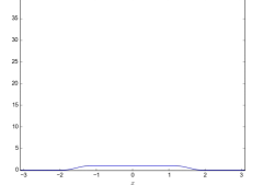
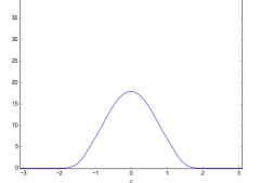
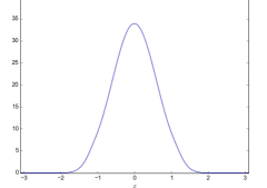
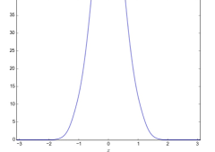
apparently has a qualitatively analogous blow up pattern, as shown by the numerical integration displayed in Figure 1. To obtain it, we use an explicit forward Euler method, with space mesh $\Delta x=10^{-3}$ and time mesh $\Delta t=10^{-3}$ on the space domain $[-3,\,3]$ and for $t\in[0,\,1.05]$.

Figure 1: Numerical integration of (2.4) for $t\in[0,\,1.05]$. The values of the $\mathbf{L^{1}}$ norm of the solution is plotted vs. time in Figure 2.

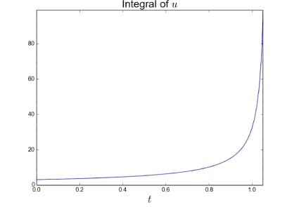
The graph of the $\mathbf{L^{1}}$ norm of the numerical solution to (2.4) is in Figure 2.

Figure 2: $\mathbf{L^{1}}$ norm of the solution to (2.4), suggesting a blow up at finite time, similar to the solution to (2.3).

It is straightforward to see that (2.4) fits into the framework of Theorem 2.2, setting

$$\begin{array}[]{rcl}N&=&1\\ n&=&1\\ m&=&1\end{array}\qquad\qquad\begin{array}[]{rcl}\varphi(t,x,u,A)&=&0\\ \Phi(t,x,u,A)&=&\psi(x)\,u\,A\,.\end{array}$$

The requirements ($\boldsymbol{\varphi}$) and ($\boldsymbol{\Phi}$) are easily seen to be satisfied.

3 A Laser Beam Cutting a Metal Plate

A thin horizontal metal plate can be cut by means of a moving vertical laser beam. More precisely, the laser energy melts the metal along a prescribed trajectory. A wind, suitably provoked around the beam, pushes the melted material downwards. For its industrial interest, this phenomenon is widely considered in the specialized literature, see [13, 14, 15, 16, 26, 27, 28, 32, 33], while information specific to the cut of aluminum are for instance in [30]. A phenomenological description of the whole process can be summarized as follows. We fix a 3D geometric framework, with the laser beam parallel to the vertical $z$ axis, see Figure 3, left. The trajectory of the laser is prescribed by the map $x_{L}=x_{L}(t)$.

\psfrag{x}{$x_{1}$}\psfrag{y}{$x_{2}$}\psfrag{z}{$z$}\includegraphics[width=142.26378pt]{SteelGeometry.eps}

\psfrag{x}{$x_{1}$}\psfrag{z}{$z$}\psfrag{hs}{$h_{s}$}\psfrag{hm}{$h_{m}$}\includegraphics[width=142.26378pt]{SteelProfile1.eps}

Figure 3: Left, reference frame with respect to the metal plate being cut. The laser beam is parallel to the $z$ axis, while the plate lies on the $z=0$ plain. Right, the distinction between the melted part $h_{m}$ and the solid one $h_{s}$.

We distinguish the height $h_{s}$ of the solid metal and that of the melted part, denoted $h_{m}$, see Figure 3, right.

A $1$D system of balance laws is used to describe the dynamics of the melted and of the solid material in [8]. Here, we present a description of this dynamics by means a $2$D system of balance laws of the form:

$$\left\{\begin{array}[]{l}\partial_{t}h_{m}+\mathop{\rm{div}}\nolimits_{x}(h_{m}\,V)=\mathcal{L}\\ \partial_{t}h_{s}=-\mathcal{L}\,.\end{array}\right.$$ (3.1)

The vector $V=V(t,x)$ describes the projection of the melted material velocity on the horizontal $(x,y)$-plane. Its modulus must depend on the wind speed $w=w(t,x)$, which is centered at the laser beam sited at $x=x_{L}(t)$. Its direction depends on the geometry of the melted metal and of the solid surface $z=H(t,x)$, where $H=h_{s}+h_{m}$. The source term $\mathcal{L}$ is directly related to the laser position and intensity: it describes the net rate at which the solid part turns into melted. Also $\mathcal{L}$ depends on the metal geometry, since the heat absorption is strictly related to the incidence angle between the moving melted metal surface and the vertical laser beam, see Figure 4, left.

Here, we posit the following assumptions:

$$V = \left(w(t,x)-\tau_{g}h_{m}\right)\;\frac{-\mathop{\rm{grad}}\nolimits_{x}(\eta*H)}{\sqrt{1+{\left\|\mathop{\rm{grad}}\nolimits_{x}(\eta*H)\right\|}^{2}}}$$ (3.2)

$$\mathcal{L} = \frac{i(t,x)}{1+{\left\|\mathop{\rm{grad}}\nolimits_{x}(\eta*H)\right\|}^{2}}\,.$$ (3.3)

The term with the coefficient $\tau_{g}$ in (3.2) is related to the shear stress, inspired by [8, 33]. The denominator in (3.2) is due to a (smooth) normalization of the direction $-\mathop{\rm{grad}}\nolimits_{x}(\eta*H)$ of the average steepest descent along the surface $z=H(t,x)$. Indeed, the convolution kernel $\eta$ is chosen smooth, compactly supported and with total mass $1$, so that $\mathop{\rm{grad}}\nolimits_{x}\left(\eta*H(t)\right)(x)$ is the average gradient at position $x$ and time $t$ of the surface $z=H(t,x)$.

In (3.3), the numerator $i=i(t,x)$ is related to the laser intensity. It can be reasonably described through a compactly supported bell shaped function centered at the location of the moving focus of the laser beam.

\psfrag{x}{$x_{1}$}\psfrag{z}{$z$}\psfrag{H}{$z=H(t,x)$}\psfrag{s}{$z=h_{s}(t,x)$}\psfrag{l}{Laser axis}\psfrag{a}{$\alpha$}\psfrag{hm}{$h_{m}$}\includegraphics[width=142.26378pt]{SteelAngle.eps}

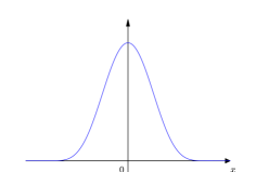
Figure 4: Left, the incidence angle $\alpha$ of the laser beam on the surface $z=H(t,x)$. Right, a possible profile for the functions $\mathcal{W}$ and $\mathcal{I}$ in (3.4).

The denominator is the squared cosine of an averaged incidence angle of the laser on the surface $z=H(t,x)$, see Figure 4, left. In fact,

$$\cos^{2}\alpha=\left(\frac{[-\partial_{x_{1}}H\quad-\partial_{x_{2}}H\quad 1]\left[\begin{array}[]{c}0\\ 0\\ 1\end{array}\right]}{{\left\|[-\partial_{x_{1}}H\quad-\partial_{x_{2}}H\quad 1]\right\|}\;{\left\|[0\quad 0\quad 1]\right\|}}\right)^{2}=\frac{1}{1+{\left\|\mathop{\rm{grad}}\nolimits_{x}H\right\|}^{2}}\,.$$

For the wind function $w=w(t,x)$ and for the laser intensity function $i=i(t,x)$ we choose a dependence on the form

$$w(t,x)=\mathcal{W}\left({\left\|x-x_{L}(t)\right\|}\right)\quad\mbox{ and }\quad i(t,x)=\mathcal{I}\left({\left\|x-x_{L}(t)\right\|}\right)$$ (3.4)

where both maps $\mathcal{W}$ and $\mathcal{I}$ have the form in Figure 4, right. More precisely, in the real setting under consideration, the diameter of the support of $\mathcal{W}$ is a few times larger than that of $\mathcal{I}$.

We stress that the present model describes how the laser beam digs a block of metal along its movement, i.e., it describes the dynamics of the melted metal and the profile of the solid material during the passing of the laser beam. At the physical level, the actual formation of the hole makes the melted material fall and, essentially, disappear. At the analytic level, the appearance of the hole causes major discontinuities that can hardly be described within a model of the form (3.1). Therefore, we provide (3.1)–(3.2)–(3.3) with an initial datum

$$h_{s}(0,x)=h_{s}^{o}\quad\mbox{ and }\quad h_{m}(x)=0$$ (3.5)

where the constant $h_{m}^{o}$ is the uniform thickness of the plate under consideration. Then, we interpret the region where $h_{s}(t,x)<0$ as the region where the cut is accomplished.

As a result we obtain the following model:

$$\left\{\begin{array}[]{l@{}}\displaystyle\partial_{t}h_{m}+\mathop{\rm{div}}\nolimits_{x}\left[\left(w(t,x)h_{m}-\tau_{g}(h_{m})^{2}\right)\frac{-\mathop{\rm{grad}}\nolimits_{x}(\eta*H)}{\sqrt{1+{\left\|\mathop{\rm{grad}}\nolimits_{x}(\eta*H)\right\|}^{2}}}\right]=\frac{i(t,x)}{1+{\left\|\mathop{\rm{grad}}\nolimits_{x}(\eta*H)\right\|}^{2}}\\ \displaystyle\partial_{t}h_{s}=-\frac{i(t,x)}{1+{\left\|\mathop{\rm{grad}}\nolimits_{x}(\eta*H)\right\|}^{2}}\\ H=h_{s}+h_{m}\end{array}\right.$$ (3.6)

To apply Theorem 2.2 to the model (3.6), a formal modification is necessary. Indeed, we introduce a cutoff function

$${\cal T}_{g}(t,x)=\tau_{g}\,\mathcal{S}\left({\left\|x-x_{L}(t)\right\|}\right)\quad\mbox{ where }\quad\mathcal{S}(\xi)=\left\{\begin{array}[]{lrcl}1&\xi&\in&[0,\,r]\\ 0&\xi&\in&\left[R,+\infty\right[\end{array}\right.$$ (3.7)

for a smooth $\mathcal{S}$ and suitable (large) $r$ and $R$, with $r<R$. We thus obtain

$$\left\{\begin{array}[]{l@{}}\displaystyle\partial_{t}h_{m}+\mathop{\rm{div}}\nolimits_{x}\left[\frac{-\left(w(t,x)h_{m}-{\cal T}_{g}(t,x)(h_{m})^{2}\right)\mathop{\rm{grad}}\nolimits_{x}(\eta*H)}{\sqrt{1+{\left\|\mathop{\rm{grad}}\nolimits_{x}(\eta*H)\right\|}^{2}}}\right]=\frac{i(t,x)}{1+{\left\|\mathop{\rm{grad}}\nolimits_{x}(\eta*H)\right\|}^{2}}\\ \displaystyle\partial_{t}h_{s}=-\frac{i(t,x)}{1+{\left\|\mathop{\rm{grad}}\nolimits_{x}(\eta*H)\right\|}^{2}}\\ H=h_{s}+h_{m}\end{array}\right.$$ (3.8)

When used with real data, the two problems (3.6) and (3.8) are indistinguishable.

Proposition 3.1.

The model (3.8) fits into (1.1) setting:

$$\begin{array}[]{@{}r@{\;}c@{\;}l}N&=&2\\ n&=&2\\ m&=&2\\ u_{1}&=&h_{m}\\ u_{2}&=&h_{s}\end{array}\qquad\vartheta(x)=\left[\begin{array}[]{cc}\partial_{x_{1}}\eta(x)&\partial_{x_{1}}\eta(x)\\ \partial_{x_{2}}\eta(x)&\partial_{x_{2}}\eta(x)\end{array}\right]\qquad\begin{array}[]{@{}r@{\;}c@{\;}l@{}}\varphi_{1}(t,x,u_{1},A)&=&\!\left(w(t,x)-{\cal T}_{g}(t,x)u_{1}\right)\frac{-u_{1}\,A}{\sqrt{1+{\left\|A\right\|}^{2}}}\\ \varphi_{2}(t,x,u_{2},A)&=&0\\ \Phi_{1}(t,x,u,A)&=&\frac{1}{\sqrt{1+{\left\|A\right\|}^{2}}}\,i(t,x)\\ \Phi_{2}(t,x,u,A)&=&-\frac{1}{\sqrt{1+{\left\|A\right\|}^{2}}}\,i(t,x)\,,\end{array}$$

where $w,i$ are defined in (3.4) and ${\cal T}_{g}$ in (3.7). Moreover, if

$$x_{L}\in(\mathbf{C^{2}}\cap\mathbf{W^{2,\infty}})([0,\widehat{T}];{\mathbb{R}}^{2})\,,\quad\mathcal{W},\mathcal{I},\mathcal{S}\in\mathbf{C_{c}^{2}}({\mathbb{R}};{\mathbb{R}})\quad\mbox{ and }\quad\eta\in\mathbf{C_{c}^{3}}({\mathbb{R}}^{2};{\mathbb{R}})$$ (3.9)

for a positive $\widehat{T}$, then, assumptions ($\boldsymbol{\varphi}$), ($\boldsymbol{\Phi}$), ($\boldsymbol{\vartheta}$) hold.

The proof is deferred to Section 5. The above Proposition 3.1 allows to apply Theorem 2.2 to model (3.8), ensuring its well posedness.

3.1 Numerical Integration

The model (3.6), fed with realistic values of the various parameters, is able to reproduce the rising of ripples. The following numerical integrations show this qualitative feature.

We use below the numerical method presented in [1], where it is proved to be convergent up to a subsequence in the case of a system of nonlocal conservation laws. As it is usual, we deal with the source terms by means of the fractional step method, see for instance [22, Section 12.1]. In other words, we use a Lax–Friedrichs type algorithm for the convective part and a first order explicit forward Euler method for the ordinary differential equations arising from the source terms.

The computational domain is the rectangle $[0,\,40]\times[-2,\,2]$, entirely contained in the metal plate to be cut (all lengths being measured in millimeters). The mesh size is $5\cdot 10^{-3}$ along both axis. The integration is computed for $t\in[0,\,1]$, time being measured in seconds.

The laser trajectory is

$$x_{L}(t)=\left\{\begin{array}[]{lrcl}(3,\,0)&t&\in[0,\,0.1]\\ \left(3+40\,(t-0.1),\,0\right)&t&\in\left]0.1,\,1\right]\end{array}\right.$$

meaning that for $t\in[0,\,0.1]$ the initial hole is drilled centered at $(3,\,0)$, in the interior of the metal plate. The speed of the laser beam, $40\frac{{\rm mm}}{{\rm sec}}$, is coherent with the data in [31], see also [8, Table 1].

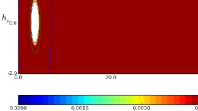
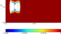
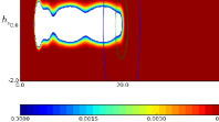
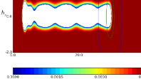
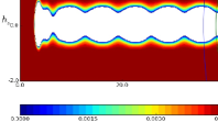
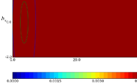
Figure 5: Numerical integration of (3.6) with the data and parameters provided in § 3.1, see [8, 31]. These are the contour plots of the solid metal level $h_{s}$ in the interval $[0,\,4.5]$ over the domain $[0,\,40]\times[-2,\,2]$ millimeters. The inner circle (appearing as an ellipse due to the different scales on the two axis) is the support of the laser beam. The outer one is the support of the wind. At time $t=0.1$, the initial hole is terminated and the laser beam starts moving rightwards. Note the formation of “ripples”, i.e., the sides of the cut are not flat but present an apparently regularly oscillating profile. Neither data nor parameters are “pulsating”.

The wind and laser functions are given by (3.4) setting

$$\begin{array}[]{rclr@{\;}c@{\;}lrcl}\mathcal{W}(\xi)&=&\displaystyle\left(1-\left(\frac{\xi}{3.6}\right)^{2}\right)^{4}&\mbox{ for }{\left\|\xi\right\|}&\leq&3.6\\ \mathcal{I}(\xi)&=&\displaystyle 2\,\left(1-\left(\frac{\xi}{1.2}\right)^{2}\right)^{6}&\mbox{ for }{\left\|\xi\right\|}&\leq&1.2\end{array}$$

corresponding to a laser beam with radius $1.2\,$mm, see [31]. The radius of the surface where the wind blows downward is $3$ times that of the laser beam. Besides, we set $\tau_{g}=4$. The convolution kernel is

$$\eta(x)=\frac{1}{\int_{{\mathbb{R}}^{2}}\tilde{\eta}(y)\mathinner{\mathrm{d}{y}}}\,\tilde{\eta}(x)\quad\mbox{ where }\quad\tilde{\eta}(x)=\left(1-\left(\frac{{\left\|x\right\|}}{2.4}\right)^{2}\right)^{3}\qquad\mbox{ for }{\left\|x\right\|}\leq 2.4\,.$$

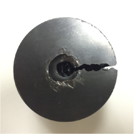
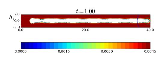
Figure 6: Left, a real piece of metal with a hole and a cut made by a laser beam. Right, the result of the numerical integration of the model (3.6) as in Figure 5, but plotted with the same scales along the two axis.

As initial datum, we choose

$$\bar{h}_{m}(x)=0\qquad\mbox{ and }\qquad\bar{h}_{s}(x)=4.5\qquad\mbox{ for all }x\in{\mathbb{R}}^{2}\,,$$

representing a flat metal plate $4.5\,$mm thick, see [31].

The result of this integration is in Figure 5, which displays the contour plot of the surface $z=h_{s}(t,x)$ remaining after the cut, restricted to the interval $[0,\,4.5]$mm. The white part corresponds to a level below $0$ and should be understood as expelled, corresponding to the cut. Remark the oscillations arisen along the sides of the cut. No parameter and no datum in the integration oscillates, nevertheless, the solution displays these sort of “ripples”.

4 Materials Flowing on a Conveyor Belt

A macroscopic model for the flow of materials along a conveyor belt is presented in [12]. The material consists of a large number of solid identical particles, called cargo. From a macroscopic point of view, the cargo state is identified by a density $\rho=\rho(t,x)$, where $t$ is time and $x\equiv(x_{1},\,x_{2})$ is the coordinate along the conveyor belt. The industrial interest behind these modeling efforts is motivated by the need of an efficient management of specific parts of the production process. A standard example is the pouring of newly produced bolts in boxes. In this case, a selector is positioned on the belt to drive the bolts in a short segment of the belt, so that at the end of the conveyor they fall in their boxes, see [12] and figure 7, left. For other references on these modeling issues, both from the microscopic and macroscopic points of view, see for instance [23], related to conveyor belts in mines, or [17, 29] and the review [19].

With the notation in [12, Section 3], a macroscopic description for the cargo dynamics is provided by the equation

$$\partial_{t}\rho+\mathop{\rm{div}}\nolimits_{x}\left(\rho\left(\boldsymbol{v^{stat}}(x)+H(\rho-\rho_{max})\,\mathcal{I}(\rho)\right)\right)=0\,.$$ (4.1)

Here, $\boldsymbol{v^{stat}}$ is the time independent velocity of the underlying conveyor belt. The fixed positive $\rho_{max}$ is the maximal cargo density and $H$ is the usual Heaviside function. The term

$$\mathcal{I}(\rho)=\varepsilon\,\frac{-\mathop{\rm{grad}}\nolimits_{x}(\eta*\rho)}{\sqrt{1+{\left\|\mathop{\rm{grad}}\nolimits_{x}(\eta*\rho)\right\|}^{2}}}$$ (4.2)

describes how the cargo velocity is modified when the maximal density is reached: particles move towards regions with lower average cargo density, $\eta$ being a $\mathbf{C_{c}^{2}}$ positive function with integral $1$, so that $\eta*\rho$ is an average cargo density. Further details are available in [12, Section 3], where (4.1) is supplied with suitable boundary conditions along the sides of the conveyor belt. The numerical study therein shows a good agreement between the solutions to (4.1) and real data.

Next, we slightly modify (4.1). The conveyor belt is described by the strip ${\left|x_{2}\right|}\leq\ell$. First, we replace the Heaviside function by a regularization

$$H^{\mu}\in\mathbf{C^{2}}({\mathbb{R}};[0,1])\quad\mbox{ with }\quad H^{\mu}(\xi)=H(\xi)\quad\forall\xi\mbox{ with }{\left|\xi\right|}>\mu\,.$$ (4.3)

Then, we modify $\boldsymbol{v^{stat}}(x)$ so that it incorporates the upper and lower conveyor boundaries. To this aim, we introduce the vector field $\boldsymbol{b}(x)\in\mathbf{C_{c}^{2}}({\mathbb{R}}^{2};{\mathbb{R}}^{2})$, see Figure 7, right,

\psfrag{ml}{$-\ell$}\psfrag{l}{$\ell$}\psfrag{x1}{$x_{1}$}\psfrag{x2}{$x_{2}$}\includegraphics[width=195.12767pt]{convBeltSel.eps}

\psfrag{ml}{$-\ell$}\psfrag{l}{$\ell$}\psfrag{x1}{$x_{1}$}\psfrag{x2}{$x_{2}$}\psfrag{d}{$\delta$}\includegraphics[width=195.12767pt]{convBelt.eps}

Figure 7: Left, a conveyor belt with a selector restricting the possible path of the carried cargo. Right, geometry and notation of the conveyor belt.

such that:

$$\begin{array}[]{r@{\;}c@{\;}r@{\qquad}r@{\;}c@{\;}l}\left(\boldsymbol{b}(x_{1},\ell)\right)_{2}&=&-\widehat{\varepsilon}\quad\forall x_{1}\in{\mathbb{R}}\,,&\left(\boldsymbol{b}(x)\right)_{1}&=&0\quad\forall x\in{\mathbb{R}}^{2}\,,\\ \left(\boldsymbol{b}(x_{1},-\ell)\right)_{2}&=&\widehat{\varepsilon}\quad\forall x_{1}\in{\mathbb{R}}\,,&\left(\boldsymbol{b}(x)\right)_{2}&=&0\quad\forall x\in{\mathbb{R}}^{2}\mbox{ with }{\left|x_{2}-\ell\right|}>\delta\mbox{ or }{\left|x_{2}+\ell\right|}>\delta\,.\end{array}$$

We therefore obtain the equation

$$\partial_{t}\rho+\mathop{\rm{div}}\nolimits_{x}\left(\rho\left(\boldsymbol{v^{stat}}(x)+\boldsymbol{b}(x)+H^{\mu}(\rho-\rho_{max})\,\mathcal{I}(\rho)\right)\right)=0$$ (4.4)

which describes the cargo dynamics along the conveyor belt. Thanks to the framework provided by Theorem 2.2, we can incorporate in the model also the cargo source and sink. Indeed, we assume that the solid particles are poured on the belt in a region, say, $R_{in}=[0,a]\times[-\ell,\ell]$ and fall out of the belt in the region $R_{out}=[L-a,L]\times[-\ell,\ell]$. To this aim, for a positive $\widehat{T}$, we introduce the source and sink functions

$$\begin{array}[]{@{}r@{\;}c@{\;}l@{\mbox{ with ~}}l@{}}\Psi_{in}&\in&\mathbf{C^{2}}([0,\widehat{T}]\times R_{in};{\mathbb{R}}^{+})\hfil\mbox{ with ~{}&\mathop{\mathrm{missing}}{spt}\Psi_{in}(t,\cdot)\subseteq R_{in}\mbox{ for all }t\in[0,\widehat{T}]\\[6.0pt] \Psi{{}_{out}}&\in&\mathbf{C^{2}}([0,\widehat{T}]\times R_{in}\times{\mathbb{R}};{\mathbb{R}}^{+})\hfil\mbox{ with ~{}&\begin{array}[]{@{}l@{}}\mathop{\mathrm{missing}}{spt}\Psi_{out}(t,\cdot,\rho)\subseteq R_{out}\mbox{ for all }t\in[0,\widehat{T}]\mbox{ and }\rho\in{\mathbb{R}}\\ \Psi_{out}(\cdot,\cdot,\rho)=0\mbox{ for all }\rho\leq 0\end{array}\end{array}}}$$ (4.5)

The function $\Psi_{in}$ is the rate at which particles are poured in $R_{in}$, while $\Psi{{}_{out}}$ describes the outflow from the belt.

We can assume that the belt is initially empty, thus we obtain the following Cauchy Problem, where we set $\boldsymbol{v}=\boldsymbol{v}^{stat}+\boldsymbol{b}$,

$$\left\{\begin{array}[]{l}\partial_{t}\rho+\mathop{\rm{div}}\nolimits_{x}\left(\rho\left(\boldsymbol{v}(x)+H^{\mu}(\rho-\rho_{max})\;\mathcal{I}(\rho)\right)\right)=\Psi_{in}(t,x)-\Psi_{out}(t,x,\rho)\\ \rho(t,0)=0\end{array}\right.$$ (4.6)

Proposition 4.1.

Fix positive $\widehat{T},\ell,L,\mu,\rho_{max},\varepsilon,\widehat{\varepsilon}$ with $\widehat{\varepsilon}>\varepsilon$. Let $\mathcal{B}=[0,L]\times[-\ell,\ell]$ be the conveyor belt. If $\boldsymbol{v}\in\mathbf{C^{2}}({\mathbb{R}}^{2};{\mathbb{R}}^{2})$ is such that

$$\begin{array}[]{rcl@{\qquad}rcl}\left(\boldsymbol{v}(0,x_{2})\right)_{1}&\geq&0\quad\forall x_{2}\in[-\ell,\ell]&\left(\boldsymbol{v}(L,x_{2})\right)_{1}&\leq&0\quad\forall x_{2}\in[-\ell,\ell]\\ \left(\boldsymbol{v}(x_{1},-\ell)\right)_{2}&\geq&\widehat{\varepsilon}\quad\forall x_{1}\in[0,L]&\left(\boldsymbol{v}(x_{1},\ell)\right)_{2}&\geq&\widehat{\varepsilon}\quad\forall x_{1}\in[0,L]\,,\end{array}$$ (4.7)

$H^{\mu}$ is as in (4.3), $\mathcal{I}$ is as in (4.2) and $\Psi_{in},\Psi_{out}$ are as in (4.5), then there exists a positive $T_{*}$ such that problem (4.6) admits a solution on the time interval $[0,T_{*}]$. Moreover, this solution is supported in $\mathcal{B}$ for all $t\in[0,T_{*}]$.

The proof is deferred at the end Section 5.

5 Technical Details

The proof of Theorem 2.2 consists of several steps. We briefly describe here the overall formal structure.

Fix a positive $T\in\widehat{I}$ and let $I=[0,T]$. Introduce the map

$$\mathcal{T}\colon(w,\tilde{u})\to u$$

where $u\equiv(u_{1},\ldots,u_{n})$ and its $i$-th component $u_{i}$ solves the nonlinear balance law

$$\left\{\begin{array}[]{l}\partial_{t}u_{i}+\mathop{\rm{div}}\nolimits_{x}\varphi_{i}(t,x,u_{i},\vartheta*w)=\Phi_{i}(t,x,u_{i},\vartheta*w)\\ u_{i}(0,x)=\tilde{u}_{i}(x)\end{array}\right.$$ (5.1)

for $i=1,\ldots,n$. By construction, solving (1.1) is equivalent to solving the fixed point problem $u=\mathcal{T}(u,\bar{u})$. The core of the proof thus consists in choosing $T$ and suitable subsets

$$\mathbb{W}\subset\mathbf{C^{0}}\left(I;\mathbf{L^{1}}({\mathbb{R}}^{N};{\mathbb{R}}^{n})\right)\quad\mbox{ and }\quad\mathbb{U}\subset\mathbf{L^{1}}({\mathbb{R}}^{N};{\mathbb{R}}^{n}),$$

see (5.2), so that

$$\left\{\begin{array}[]{ll@{\qquad}l}\mbox{(i)}&\forall(w,\tilde{u})\in\mathbb{W}\times\mathbb{U},&\mathcal{T}(w,\tilde{u})\mbox{ is well defined,}\\ \mbox{(ii)}&\forall(w,\tilde{u})\in\mathbb{W}\times\mathbb{U},&\mathcal{T}(w,\tilde{u})\mbox{ is in }\mathbb{W},\\ \mbox{(iii)}&\forall\tilde{u}\in\mathbb{U},&w\to\mathcal{T}(w,\tilde{u})\mbox{ is a contraction,}\\ \mbox{(iv)}&\forall w\in\mathbb{W},&\tilde{u}\to\mathcal{T}(w,\tilde{u})\mbox{ is Lipschitz continuous,}\\ \mbox{(v)}&\forall(w,\tilde{u})\in\mathbb{W}\times\mathbb{U},&t\to\left(\mathcal{T}(w,\tilde{u})\right)(t)\mbox{ is continuous.}\end{array}\right.$$

Steps 1 and 2 in the proof below give (i). The a priori bounds proved in steps 3, 4, 5 and 6 ensure (ii). The key estimate (5.19), which has the form

$${\left\|\mathcal{T}(w^{\prime},\tilde{u})-\mathcal{T}(w^{\prime\prime},\tilde{u})\right\|}_{\mathbf{C^{0}}(I;\mathbf{L^{1}}({\mathbb{R}}^{N};{\mathbb{R}}^{n}))}\leq\mathinner{\mathcal{O}(1)}\;T\;{\left\|w^{\prime}-w^{\prime\prime}\right\|}_{\mathbf{C^{0}}(I;\mathbf{L^{1}}({\mathbb{R}}^{N};{\mathbb{R}}^{n}))}$$

and is proved in Step 7, shows that (iii) holds for $T$ small. The statement (iv) is obtained in Step 9 through an estimate of the form

$${\left\|\mathcal{T}(w,\tilde{u}^{\prime})-\mathcal{T}(w,\tilde{u}^{\prime\prime})\right\|}_{\mathbf{C^{0}}(I;\mathbf{L^{1}}({\mathbb{R}}^{N};{\mathbb{R}}^{n}))}\leq\mathinner{\mathcal{O}(1)}\;{\left\|\tilde{u}^{\prime}-\tilde{u}^{\prime\prime}\right\|}_{\mathbf{L^{1}}({\mathbb{R}}^{N};{\mathbb{R}}^{n})}\,,$$

see (5.20). Finally, (v) is the content of Step 4, see (5.10)–(5.10), used also in the proof of (ii).

Once the statements (i), $\ldots$, (v) are obtained, the proof of Theorem 2.2 is essentially completed.

Proof of Theorem 2.2.  Throughout, we use the standard properties of the convolution product and, in particular, the following bounds. If $\vartheta$ satisfies ($\boldsymbol{\vartheta}$) and $u\in\mathbf{L^{1}}({\mathbb{R}}^{N};{\mathbb{R}}^{n})$, then

$${\left\|\vartheta*u\right\|}_{\mathbf{L^{\infty}}(I\times{\mathbb{R}}^{N};{\mathbb{R}}^{n})}\leq{\left\|\vartheta\right\|}_{\mathbf{L^{\infty}}({\mathbb{R}}^{N};{\mathbb{R}}^{m\times n})}\;{\left\|u\right\|}_{\mathbf{C^{0}}(I;\mathbf{L^{1}}({\mathbb{R}}^{N};{\mathbb{R}}))}$$

which is a straightforward generalization, for instance, of [6, Theorem IV.15]. By ($\boldsymbol{\vartheta}$), without any loss of generality, we may assume that

$${\left\|\vartheta_{ji}\right\|}_{\mathbf{L^{1}}({\mathbb{R}}^{N};{\mathbb{R}})}\leq 1/n\quad\mbox{ for all }\quad j=1,\ldots,m\quad\mbox{ and }\quad i=1,\ldots,n\,.$$

This requirement simplifies several estimates below, since it ensures that

$$u_{i}(x)\in\mathcal{U}_{U}\mbox{ for all }i=1,\ldots,n\quad\mbox{ and }\quad x\in{\mathbb{R}}^{N}\quad\Rightarrow\quad(\vartheta*u)(x)\in\mathcal{U}_{U}^{m}\quad\mbox{ for all }\quad x\in{\mathbb{R}}^{N}\,.$$

1: Notation and Definition of $\mathcal{T}$.

Fix positive $K$, $U$, $\bar{U}$, $R$ and $\bar{R}$ with

$${\left\|\bar{u}\right\|}_{\mathbf{L^{1}}({\mathbb{R}}^{N};{\mathbb{R}}^{n})}\leq\bar{R}<R\,,\quad{\left\|\bar{u}\right\|}_{\mathbf{L^{\infty}}({\mathbb{R}}^{N};{\mathbb{R}}^{n})}\leq\bar{U}<U\quad\mbox{ and }\quad\mathop{\mathrm{missing}}{TV}(\bar{u})<K\,.$$

Introduce the $\mathbf{L^{1}}$ closed sphere centered at the initial datum $\bar{u}$ with radius $R$ and its intersection with $\mathbf{BV}$ as follows:

$$B_{\mathbf{L^{1}}}(\bar{u},R,U) = \left\{u\in\mathbf{L^{1}}({\mathbb{R}}^{N};{\mathbb{R}}^{n})\colon{\left\|u-\bar{u}\right\|}_{\mathbf{L^{1}}({\mathbb{R}}^{N};{\mathbb{R}}^{n})}\leq R\mbox{ and }u(x)\in\mathcal{U}_{U}^{n}\right\}$$

$$B_{\mathbf{L^{1}}\cap\mathbf{BV}}(\bar{u},\bar{R},\bar{U},K) = \left\{u\in B_{\mathbf{L^{1}}}(\bar{u},\bar{R},\bar{U})\colon\mathop{\mathrm{missing}}{TV}(u)\leq K\right\}.$$

For any positive $T\in\widehat{I}$, denote $I=[0,T]$ and define the map

$$\begin{array}[]{@{}c@{\;}c@{\;}ccccc@{}}\mathcal{T}&\colon&\mathbf{C^{0}}\left(I;B_{\mathbf{L^{1}}}(\bar{u},R,U)\right)&\times&B_{\mathbf{L^{1}}\cap\mathbf{BV}}(\bar{u},\bar{R},\bar{U},K)&\to&\mathbf{C^{0}}\left(I;B_{\mathbf{L^{1}}}(\bar{u},R,U)\right)\\ &&w&,&\tilde{u}&\to&u\end{array}$$ (5.2)

where the function $u\equiv(u_{1},\ldots,u_{n})$ is such that for $i=1,\ldots,n$, $u_{i}$ solves (5.1). We equip the Banach space $\mathbf{C^{0}}\left(I;\mathbf{L^{1}}({\mathbb{R}}^{N};{\mathbb{R}}^{n})\right)$ with its natural norm

$${\left\|u\right\|}_{\mathbf{C^{0}}\left(I;\mathbf{L^{1}}({\mathbb{R}}^{N};{\mathbb{R}}^{n})\right)}=\sup_{t\in I}{\left\|u(t)\right\|}_{\mathbf{L^{1}}({\mathbb{R}}^{N};{\mathbb{R}}^{n})}\,,$$

and the metric space $B_{\mathbf{L^{1}}\cap\mathbf{BV}}(\bar{u},r,K)$ with the $\mathbf{L^{1}}$–distance. Denote below

$$\Omega_{T}=I\times{\mathbb{R}}^{N}\times{\mathbb{R}}\quad\mbox{ and }\quad\Omega_{T}^{U}=I\times{\mathbb{R}}^{N}\times\mathcal{U}_{U}\,.$$

Moreover, we set

$$\Lambda(t,U)={\left\|\lambda(\cdot,\cdot,U)\right\|}_{\mathbf{L^{1}}([0,t]\times{\mathbb{R}}^{N};{\mathbb{R}})}$$ (5.3)

so that $\Lambda(\cdot,U)\in\mathbf{C^{0}}(\widehat{I};{\mathbb{R}})$ is non decreasing, bounded and $\Lambda(0,U)=0$ for all $U\in{\mathbb{R}}^{+}$.

Throughout, we denote by $C$ a quantity dependent only on $\lambda$ and on the norms in ($\boldsymbol{\varphi}$), ($\boldsymbol{\Phi}$) and ($\boldsymbol{\vartheta}$), but independent of $T$, $R$, $U$, $\bar{R}$, $\bar{U}$ and $K$. Similarly, $C_{U}$ is a constant depending only on ${\left\|\varphi\right\|}_{\mathbf{W^{2,\infty}}(I\times{\mathbb{R}}^{N}\times\mathcal{U}_{U}\times\mathcal{U}_{U}^{m};{\mathbb{R}}^{n\times m})}$ and on ${\left\|\Phi\right\|}_{\mathbf{W^{1,\infty}}(I\times{\mathbb{R}}^{N}\times\mathcal{U}_{U}\times\mathcal{U}_{U}^{m};{\mathbb{R}}^{n})}$.

2: Problem (5.1) Admits a Solution.

Note that if $i\neq j$, equation (5.1) is decoupled from the analogous equation for $u_{j}$. Therefore, we want to apply the classical result by Kružkov [20, Theorem 1], see also [21, Theorem 2.1], to each equation in (5.1), setting iteratively for $i=1,\ldots,n$

$$f(t,x,u)=\varphi_{i}\left(t,x,u,(\vartheta*w)(t,x)\right)\quad\mbox{ and }\quad F(t,x,u)=\Phi_{i}\left(t,x,u,(\vartheta*w)(t,x)\right)\,.$$

To this aim, we check that the assumption (H1*) in [21, Theorem 2.1], see also [20, Theorem 1], is satisfied.

(H1*)

$f\in\mathbf{C^{0}}(\Omega_{T};{\mathbb{R}}^{N})$ holds by ($\boldsymbol{\varphi}$) and ($\boldsymbol{\vartheta}$), since $w\in\mathbf{C^{0}}\left(I;\mathbf{L^{1}}({\mathbb{R}}^{N};{\mathbb{R}}^{n})\right)$.

$F\in\mathbf{C^{0}}(\Omega_{T};{\mathbb{R}})$ holds by ($\boldsymbol{\Phi}$) and ($\boldsymbol{\vartheta}$), since $w\in\mathbf{C^{0}}\left(I;\mathbf{L^{1}}({\mathbb{R}}^{N};{\mathbb{R}}^{n})\right)$.

$f$ has continuous derivatives $\partial_{u}f$, $\partial_{u}\mathop{\rm{grad}}\nolimits_{x}f$, $\mathop{\rm{grad}}\nolimits_{x}^{2}f$, by ($\boldsymbol{\varphi}$) and ($\boldsymbol{\vartheta}$).

$F$ has continuous derivatives $\partial_{u}F$ and $\mathop{\rm{grad}}\nolimits_{x}F$ by ($\boldsymbol{\Phi}$) and ($\boldsymbol{\vartheta}$).

$\partial_{u}f\in\mathbf{L^{\infty}}(\Omega_{U}^{T};{\mathbb{R}})$ by ($\boldsymbol{\varphi}$).

$(F-\mathop{\rm{div}}\nolimits_{x}f)\in\mathbf{L^{\infty}}(\Omega_{T}^{U};{\mathbb{R}})$ by ($\boldsymbol{\varphi}$) and ($\boldsymbol{\Phi}$).

$\partial_{u}(F-\mathop{\rm{div}}\nolimits_{x}f)\in\mathbf{L^{\infty}}(\Omega_{T}^{U};{\mathbb{R}})$ by ($\boldsymbol{\varphi}$) and ($\boldsymbol{\Phi}$).

Therefore, problem (5.1) admits a solution $u\in\mathbf{L^{\infty}}\left(I;\mathbf{L^{1}_{loc}}({\mathbb{R}}^{N};{\mathbb{R}}^{n})\right)$.

3: Total Variation Estimate.

We want to apply [10, Theorem 2.5] as refined in [21, Theorem 2.2]. To this aim, we verify (H2*) in [21, § 2].

(H2*)

$\mathop{\rm{grad}}\nolimits_{x}\partial_{u}f\in\mathbf{L^{\infty}}(\Omega_{T}^{U};{\mathbb{R}}^{N\times N})$ by ($\boldsymbol{\varphi}$) and ($\boldsymbol{\vartheta}$).

$\partial_{u}F\in\mathbf{L^{\infty}}(\Omega_{T}^{U};{\mathbb{R}})$ since $\partial_{u}F=\partial_{u_{i}}\varphi_{i}$ and since ($\boldsymbol{\Phi}$) holds.

$\int_{I}\int_{{\mathbb{R}}^{N}}{\left\|\mathop{\rm{grad}}\nolimits_{x}(F-\mathop{\rm{div}}\nolimits_{x}f)(t,x,\cdot)\right\|}_{\mathbf{L^{\infty}}(\mathcal{U}_{U};{\mathbb{R}}^{N})}\mathinner{\mathrm{d}{x}}\mathinner{\mathrm{d}{t}}<+\infty$: indeed, note that the inequality ${\left\|\mathop{\rm{grad}}\nolimits_{x}F(t,x,\cdot)\right\|}_{\mathbf{L^{\infty}}(\mathcal{U}_{U};{\mathbb{R}}^{N})}\leq\lambda(t,x,U)$ holds by ($\boldsymbol{\Phi}$). Moreover,

$$\begin{array}[]{rcl}\mathop{\rm{div}}\nolimits_{x}f(t,x,u)&=&\mathop{\rm{div}}\nolimits_{x}\varphi_{i}\left(t,x,u,(\vartheta*w)(t,x)\right)\\ &&+\mathop{\rm{grad}}\nolimits_{A}\varphi_{i}\left(t,x,u,(\vartheta*w)(t,x)\right)\;\mathop{\rm{div}}\nolimits_{x}(\vartheta*w)(t,x)\end{array}$$ (5.4)

and passing to the gradient

$$\mathop{\rm{grad}}\nolimits_{x}\mathop{\rm{div}}\nolimits_{x}f(t,x,u)$$

$$= \mathop{\rm{grad}}\nolimits_{x}\mathop{\rm{div}}\nolimits_{x}\varphi_{i}\left(t,x,u,(\vartheta*w)(t,x)\right)$$

$$+\mathop{\rm{grad}}\nolimits_{A}\mathop{\rm{div}}\nolimits_{x}\varphi_{i}\left(t,x,u,(\vartheta*w)(t,x)\right)\;\mathop{\rm{grad}}\nolimits_{x}(\vartheta*w)(t,x)$$

$$+\mathop{\rm{grad}}\nolimits_{x}\mathop{\rm{grad}}\nolimits_{A}\varphi_{i}\left(t,x,u,(\vartheta*w)(t,x)\right)\;\mathop{\rm{div}}\nolimits_{x}(\vartheta*w)(t,x)$$

$$+\mathop{\rm{grad}}\nolimits_{A}^{2}\varphi_{i}\left(t,x,u,(\vartheta*w)(t,x)\right)\;\mathop{\rm{grad}}\nolimits_{x}(\vartheta*w)(t,x)\;\mathop{\rm{div}}\nolimits_{x}(\vartheta*w)(t,x)$$

$$+\mathop{\rm{grad}}\nolimits_{A}\varphi_{i}\left(t,x,u,(\vartheta*w)(t,x)\right)\;\mathop{\rm{grad}}\nolimits_{x}\mathop{\rm{div}}\nolimits_{x}(\vartheta*w)(t,x)\,,$$

so that, using the standard properties of the convolution and ($\boldsymbol{\varphi}$)

$${\left\|\mathop{\rm{grad}}\nolimits_{x}\mathop{\rm{div}}\nolimits_{x}f(t,x,u)\right\|} \leq (1+3\,C_{U}\,R\,T+C_{U}\,R^{2}\,T^{2})\;\lambda(t,x,U)$$

$$\leq C_{U}\;(1+R\,T+R^{2}\,T^{2})\;\lambda(t,x,U)$$

and hence, using ($\boldsymbol{\varphi}$), ($\boldsymbol{\Phi}$) and (5.3),

$$\int_{I}\int_{{\mathbb{R}}^{N}}{\left\|\mathop{\rm{grad}}\nolimits_{x}(F-\mathop{\rm{div}}\nolimits_{x}f)(t,x,\cdot)\right\|}_{\mathbf{L^{\infty}}(\mathcal{U}_{U};{\mathbb{R}}^{N})}\mathinner{\mathrm{d}{x}}\mathinner{\mathrm{d}{t}}$$ (5.5)

$$\leq \int_{I}\int_{{\mathbb{R}}^{N}}\left({\left\|\mathop{\rm{grad}}\nolimits_{x}F(t,x,\cdot)\right\|}_{\mathbf{L^{\infty}}(\mathcal{U}_{U};{\mathbb{R}}^{N})}+{\left\|\mathop{\rm{grad}}\nolimits_{x}\mathop{\rm{div}}\nolimits_{x}f(t,x,\cdot)\right\|}_{\mathbf{L^{\infty}}(\mathcal{U}_{U};{\mathbb{R}}^{N})}\right)\mathinner{\mathrm{d}{x}}\mathinner{\mathrm{d}{t}}$$

$$\leq \int_{I}\int_{{\mathbb{R}}^{N}}\left(\lambda(t,x,U)+C_{U}\;(1+R\,T+R^{2}\,T^{2})\,\lambda(t,x,U)\right)\mathinner{\mathrm{d}{x}}\mathinner{\mathrm{d}{t}}$$

$$= C_{U}\;(1+R\,T+R^{2}\,T^{2})\;\Lambda(T,U)\,.$$

To apply [21, Theorem 2.5], with reference to [21, (2.6)] compute first

$$\mathop{\rm{grad}}\nolimits_{x}\partial_{u}f(t,x,u) = \mathop{\rm{grad}}\nolimits_{x}\partial_{u}\varphi_{i}\left(t,x,u,(\vartheta*w)(t,x)\right)$$

$$+\mathop{\rm{grad}}\nolimits_{A}\partial_{u}\varphi_{i}\left(t,x,u,(\vartheta*w)(t,x)\right)\mathop{\rm{grad}}\nolimits_{x}(\vartheta*w)(t,x)$$

so that

$${\left\|\mathop{\rm{grad}}\nolimits_{x}\partial_{u}f\right\|}_{\mathbf{L^{\infty}}(I\times{\mathbb{R}}^{N}\times\mathcal{U}_{U};{\mathbb{R}}^{N\times N})}\leq C_{U}+C_{U}\,C\,R\,T\leq C_{U}\,(1+C\,R\,T)$$

and

$$\kappa_{0}^{*} = (2N+1){\left\|\mathop{\rm{grad}}\nolimits_{x}\partial_{u}f\right\|}_{\mathbf{L^{\infty}}(I\times{\mathbb{R}}^{N}\times\mathcal{U}_{U};{\mathbb{R}}^{N\times N})}+{\left\|\partial_{u}F\right\|}_{\mathbf{L^{\infty}}(I\times{\mathbb{R}}^{N}\times\mathcal{U}_{U};{\mathbb{R}})}$$ (5.6)

$$\leq (2N+1)\,C_{U}\,(1+C\,R\,T)+C_{U}$$

$$\leq C\;C_{U}\;(1+R\,T)\,.$$

Denoting $W_{N}=\int_{0}^{\pi/2}(\cos\vartheta)^{N}\mathinner{\mathrm{d}{\vartheta}}$, use (5.5), (5.6) to obtain, for all $t\in I$,

$$\mathop{\mathrm{missing}}{TV}\left(u_{i}(t)\right) \leq \mathop{\mathrm{missing}}{TV}(\tilde{u})e^{\kappa_{0}^{*}t}+N\,W_{N}\!\int_{I}\!e^{\kappa_{0}^{*}(t-\tau)}\!\!\int_{{\mathbb{R}}^{N}}{\left\|\mathop{\rm{grad}}\nolimits_{x}(F-\mathop{\rm{div}}\nolimits_{x}f)(\tau,x,\cdot)\right\|}_{\mathbf{L^{\infty}}(\mathcal{U}_{U};{\mathbb{R}}^{N})}\mathinner{\mathrm{d}{x}}\mathinner{\mathrm{d}{\tau}}$$ (5.7)

$$\leq \left(\mathop{\mathrm{missing}}{TV}(\tilde{u})+N\,W_{N}\int_{I}\int_{{\mathbb{R}}^{N}}{\left\|\mathop{\rm{grad}}\nolimits_{x}(F-\mathop{\rm{div}}\nolimits_{x}f)(\tau,x,\cdot)\right\|}_{\mathbf{L^{\infty}}(\mathcal{U}_{U};{\mathbb{R}}^{N})}\mathinner{\mathrm{d}{x}}\mathinner{\mathrm{d}{\tau}}\right)e^{\kappa_{0}^{*}t}$$

$$\leq \left(K+C\,C_{U}\,(1+R\,T+R^{2}\,T^{2})\;\Lambda(T,U)\right)e^{CC_{U}(1+RT)T}\,.$$

4: $\mathbf{L^{1}}$ Continuity in Time

We use [21, Corollary 2.4]. To this aim, verify first that $f,F$ satisfy (H3*).

(H3*)

$\partial_{u}f\in\mathbf{L^{\infty}}(\Omega^{U}_{T};{\mathbb{R}}^{N})$, already verified in (H1*).

$\partial_{u}F\in\mathbf{L^{\infty}}(\Omega^{U}_{T};{\mathbb{R}})$, already verified in (H2*).

$\int_{I}\int_{{\mathbb{R}}^{N}}{\left\|(F-\mathop{\rm{div}}\nolimits_{x}f)(t,x,\cdot)\right\|}_{\mathbf{L^{\infty}}(\mathcal{U}_{U};{\mathbb{R}})}\mathinner{\mathrm{d}{x}}\mathinner{\mathrm{d}{t}}<+\infty$: use (5.4), ($\boldsymbol{\varphi}$) and ($\boldsymbol{\Phi}$) to obtain the bound

$$\int_{I}\int_{{\mathbb{R}}^{N}}{\left\|(F-\mathop{\rm{div}}\nolimits_{x}f)(t,x,\cdot)\right\|}_{\mathbf{L^{\infty}}(\mathcal{U}_{U};{\mathbb{R}})}\mathinner{\mathrm{d}{x}}\mathinner{\mathrm{d}{t}}$$ (5.8)

$$\leq \int_{I}\int_{{\mathbb{R}}^{N}}{\left\|F(t,x,\cdot)\right\|}_{\mathbf{L^{\infty}}(\mathcal{U}_{U};{\mathbb{R}})}\mathinner{\mathrm{d}{x}}\mathinner{\mathrm{d}{t}}+\int_{I}\int_{{\mathbb{R}}^{N}}{\left\|\mathop{\rm{div}}\nolimits_{x}f(t,x,\cdot)\right\|}_{\mathbf{L^{\infty}}(\mathcal{U}_{U};{\mathbb{R}})}\mathinner{\mathrm{d}{x}}\mathinner{\mathrm{d}{t}}$$

$$\leq \Lambda(T,U)+\int_{I}\int_{{\mathbb{R}}^{N}}{\left\|\mathop{\rm{div}}\nolimits_{x}\varphi\left(t,x,\cdot,(\vartheta*w)(t,x)\right)\right\|}_{\mathbf{L^{\infty}}(\mathcal{U}_{U};{\mathbb{R}})}\mathinner{\mathrm{d}{x}}\mathinner{\mathrm{d}{t}}$$

$$+\int_{I}\int_{{\mathbb{R}}^{N}}{\left\|\mathop{\rm{grad}}\nolimits_{A}\varphi\left(t,x,\cdot,(\vartheta*w)(t,x)\right)\right\|}_{\mathbf{L^{\infty}}(\mathcal{U}_{U};{\mathbb{R}})}\mathinner{\mathrm{d}{x}}\mathinner{\mathrm{d}{t}}$$

$$\qquad\times{\left\|\mathop{\rm{div}}\nolimits_{x}\vartheta\right\|}_{\mathbf{L^{\infty}}(I\times{\mathbb{R}}^{N};{\mathbb{R}}^{n})}{\left\|w\right\|}_{\mathbf{C^{0}}(I;\mathbf{L^{1}}({\mathbb{R}}^{N};{\mathbb{R}}))}$$

$$\leq \Lambda(T,U)+\Lambda(T,U)\left(1+{\left\|\mathop{\rm{div}}\nolimits_{x}\vartheta\right\|}_{\mathbf{L^{\infty}}(I\times{\mathbb{R}}^{N};{\mathbb{R}}^{n})}{\left\|w\right\|}_{\mathbf{C^{0}}(I;\mathbf{L^{1}}({\mathbb{R}}^{N};{\mathbb{R}}))}\right)$$

$$= C\,(1+R\,T)\,\Lambda(T,U)\,.$$

Repeating the same computations on the time interval between $s$ and $t$, by ($\boldsymbol{\varphi}$), [21, (2.8)], (5.7) and (5.8), for all $t,s\in I$,

$${\left\|u_{i}(t)-u_{i}(s)\right\|}_{\mathbf{L^{1}}({\mathbb{R}}^{N};{\mathbb{R}})}$$ (5.10)

$$\leq \!\!{\left|\int_{s}^{t}\int_{{\mathbb{R}}^{N}}{\left\|(F-\mathop{\rm{div}}\nolimits_{x}f)(\tau,x,\cdot)\right\|}_{\mathbf{L^{\infty}}(\mathcal{U}_{U};{\mathbb{R}})}\mathinner{\mathrm{d}{x}}\right|}+{\left|t-s\right|}\;{\left\|\partial_{u}f\right\|}_{\mathbf{L^{\infty}}(I\times{\mathbb{R}}^{N}\times\mathcal{U}_{U},{\mathbb{R}})}\;\sup_{\tau\in I}\mathop{\mathrm{missing}}{TV}\left(u_{i}(\tau)\right)$$

$$\leq \!\!C(1+RT){\left|\Lambda(t,U)-\Lambda(s,U)\right|}$$

$$+C{\left|t-s\right|}\!\left[K+C(1+RT+R^{2}T^{2})\Lambda(T,U)\right]\!e^{CC_{U}(1+RT)T}$$

proving the uniform $\mathbf{L^{1}}$–continuity in time of the map $t\to u_{i}(t)$, where $u=\mathcal{T}(w,\tilde{u})$.

5: $\mathbf{L^{\infty}}$ Bound

Passing to the limit $\varepsilon\to 0$ in the classical estimate [20, Formula (4.6)], we have that, using [20, Formulæ (4.1), (4.2) and 4) in § 4], ${\left|u(t,x)\right|}\leq(M_{o}+c_{o}T)e^{c_{1}T}$, where

$$M_{o} = {\left\|\bar{u}(x)\right\|}_{\mathbf{L^{\infty}}{({\mathbb{R}}^{N};{\mathbb{R}})}}$$

$$\leq \bar{R}\,.$$

$$c_{o} = {\left\|\mathop{\rm{div}}\nolimits_{x}f(\cdot,\cdot,0)-F(\cdot,\cdot,0)\right\|}_{\mathbf{L^{\infty}}(I\times{\mathbb{R}}^{N};{\mathbb{R}})}$$

$$\leq {\left\|\mathop{\rm{div}}\nolimits_{x}\varphi_{i}\left(\cdot,\cdot,0,(\vartheta*w)(\cdot,\cdot)\right)\right\|}_{\mathbf{L^{\infty}}(I\times{\mathbb{R}}^{N};{\mathbb{R}})}$$

$$+{\left\|\mathop{\rm{grad}}\nolimits_{A}\varphi_{i}\left(\cdot,\cdot,0,(\vartheta*w)(\cdot,\cdot)\right)\;\mathop{\rm{div}}\nolimits_{x}(\vartheta*w)(\cdot,\cdot)\right\|}_{\mathbf{L^{\infty}}(I\times{\mathbb{R}}^{N};{\mathbb{R}})}$$

$$+{\left\|\Phi\left(\cdot,\cdot,0,(\vartheta*w)(\cdot,\cdot)\right)\right\|}_{\mathbf{L^{\infty}}(I\times{\mathbb{R}}^{N};{\mathbb{R}})}$$

$$\leq C_{U}+C_{U}\,C\,R\,T+C_{U}$$

$$\leq C\,C_{U}\,(1+R\,T)\,.$$

$$c_{1} = \sup_{I\times{\mathbb{R}}^{N}\times\mathcal{U}_{U}}\left(-\partial_{u}\mathop{\rm{div}}\nolimits_{x}f(t,x,u)+\partial_{u}F(t,x,u)\right)$$

$$\leq {\left\|\partial_{u}\mathop{\rm{div}}\nolimits_{x}\varphi_{i}\left(\cdot,\cdot,\cdot,(\vartheta*w)(\cdot,\cdot)\right)\right\|}_{\mathbf{L^{\infty}}(I\times{\mathbb{R}}^{N}\times\mathcal{U}_{U};{\mathbb{R}})}$$

$$+{\left\|\partial_{u}\mathop{\rm{grad}}\nolimits_{A}\varphi_{i}\left(\cdot,\cdot,\cdot,(\vartheta*w)(\cdot,\cdot)\right)\;\mathop{\rm{div}}\nolimits_{x}(\vartheta*w)(\cdot,\cdot)\right\|}_{\mathbf{L^{\infty}}(I\times{\mathbb{R}}^{N}\times\mathcal{U}_{U};{\mathbb{R}})}$$

$$+{\left\|\partial_{u}\Phi\left(\cdot,\cdot,\cdot,(\vartheta*w)(\cdot,\cdot)\right)\right\|}_{\mathbf{L^{\infty}}(I\times{\mathbb{R}}^{N}\times\mathcal{U}_{U};{\mathbb{R}})}$$

$$\leq C_{U}+C_{U}\,C\,R\,T+C_{U}$$

$$\leq C\,C_{U}\,(1+R\,T)\,.$$

Therefore,

$${\left\|u\right\|}_{\mathbf{L^{\infty}}(I\times{\mathbb{R}}^{N};{\mathbb{R}})}\leq\left(\bar{R}+C\,C_{U}\,(1+R\,T)T\right)\exp\left(C\,C_{U}\,(1+R\,T)T\right)\,.$$ (5.11)

6: $\mathcal{T}$ is Well Defined

Apply (5.10)–(5.10) with $s=0$, obtaining that for all $t\in I$

$${\left\|u_{i}(t)-\bar{u}_{i}\right\|}_{\mathbf{L^{1}}({\mathbb{R}}^{N};{\mathbb{R}})} \leq {\left\|u_{i}(t)-\tilde{u}_{i}\right\|}_{\mathbf{L^{1}}({\mathbb{R}}^{N};{\mathbb{R}})}+{\left\|\tilde{u}_{i}-\bar{u}_{i}\right\|}_{\mathbf{L^{1}}({\mathbb{R}}^{N};{\mathbb{R}})}$$

$$\leq C(1+RT)\Lambda(T)+CT\left[K+C(1+RT+R^{2}T^{2})\Lambda(T)\right]e^{C(1+RT)T}+\bar{R}\,.$$

This inequality, together with (5.11), ensures that if $T$ is sufficiently small, $u(t)=\left(\mathcal{T}(w,\tilde{u})\right)(t)\in B_{\mathbf{L^{1}}}(\bar{u},R)$ for all $t\in I$. This estimate, together with what was proved at 2 and 4, ensures that $\mathcal{T}(w,\tilde{u})\in\mathbf{C^{0}}\left(I;\mathbf{L^{1}}({\mathbb{R}}^{N};{\mathbb{R}}^{n})\right)$ for any $\tilde{u}\in B_{\mathbf{L^{1}}\cap\mathbf{BV}}(\bar{u},r,K)$.

7: $\mathcal{T}$ is a Contraction.

Here we use the stability result [8, Theorem 2.6] as refined in [21, Theorem 2.5]. To this aim, for $w^{\prime},w^{\prime\prime}\in\mathbf{C^{0}}\left(I;\mathbf{L^{1}}({\mathbb{R}}^{N};{\mathbb{R}}^{n})\right)$, call $f^{\prime},f^{\prime\prime},F^{\prime},F^{\prime\prime}$ the corresponding fluxes and sources. We first verify that $f^{\prime}-f^{\prime\prime}$ and $F^{\prime}-F^{\prime\prime}$ satisfy (H3*).

(H3*)

$\partial_{u}(f^{\prime}-f^{\prime\prime})\in\mathbf{L^{\infty}}(\Omega_{T}^{U};{\mathbb{R}}^{N})$ is proved as in (H1*).

$\partial_{u}(F^{\prime}-F^{\prime\prime})\in\mathbf{L^{\infty}}(\Omega_{T}^{U};{\mathbb{R}})$ is proved as in (H2*).

Using ($\boldsymbol{\Phi}$) and (5.4),

$$\int_{I}\int_{{\mathbb{R}}^{N}}{\left\|(F^{\prime}-F^{\prime\prime})-\mathop{\rm{div}}\nolimits_{x}(f^{\prime}-f^{\prime\prime})(t,x,\cdot)\right\|}_{\mathbf{L^{\infty}}(\mathcal{U}_{U};{\mathbb{R}})}\mathinner{\mathrm{d}{x}}\mathinner{\mathrm{d}{t}}$$

$$\leq \int_{I}\int_{{\mathbb{R}}^{N}}{\left\|(F^{\prime}-F^{\prime\prime})(t,x,\cdot)\right\|}_{\mathbf{L^{\infty}}(\mathcal{U}_{U};{\mathbb{R}})}\mathinner{\mathrm{d}{x}}\mathinner{\mathrm{d}{t}}$$

$$+ \int_{I}\int_{{\mathbb{R}}^{N}}{\left\|\mathop{\rm{div}}\nolimits_{x}(f^{\prime}-f^{\prime\prime})(t,x,\cdot)\right\|}_{\mathbf{L^{\infty}}(\mathcal{U}_{U};{\mathbb{R}})}\mathinner{\mathrm{d}{x}}\mathinner{\mathrm{d}{t}}$$

$$\leq \int_{I}\int_{{\mathbb{R}}^{N}}{\left\|\Phi_{i}\left(t,x,\cdot,(\vartheta*w^{\prime})(t,x)\right)-\Phi_{i}\left(t,x,\cdot,(\vartheta*w^{\prime\prime})(t,x)\right)\right\|}_{\mathbf{L^{\infty}}(\mathcal{U}_{U};{\mathbb{R}})}\mathinner{\mathrm{d}{x}}\mathinner{\mathrm{d}{t}}$$

$$+ \int_{I}\int_{{\mathbb{R}}^{N}}{\left\|\mathop{\rm{div}}\nolimits_{x}\left[\varphi_{i}\left(t,x,\cdot,(\vartheta*w^{\prime})(t,x)\right)-\varphi_{i}\left(t,x,\cdot,(\vartheta*w^{\prime\prime})(t,x)\right)\right]\right\|}_{\mathbf{L^{\infty}}(\mathcal{U}_{U};{\mathbb{R}})}\mathinner{\mathrm{d}{x}}\mathinner{\mathrm{d}{t}}$$

$$+ \int_{I}\int_{{\mathbb{R}}^{N}}\Big{\|}\mathop{\rm{grad}}\nolimits_{A}\varphi_{i}\left(t,x,\cdot,(\vartheta*w^{\prime})(t,x)\right)\mathop{\rm{div}}\nolimits_{x}(\vartheta*w^{\prime})(t,x)$$

$$\qquad\qquad\qquad-\mathop{\rm{grad}}\nolimits_{A}\varphi_{i}\left(t,x,\cdot,(\vartheta*w^{\prime\prime})(t,x)\right)\mathop{\rm{div}}\nolimits_{x}(\vartheta*w^{\prime\prime})(t,x)\Big{\|}_{\mathbf{L^{\infty}}(\mathcal{U}_{U};{\mathbb{R}})}\mathinner{\mathrm{d}{x}}\mathinner{\mathrm{d}{t}}$$

$$\leq {\left\|\Phi\right\|}_{\mathbf{W^{1,\infty}}(I\times{\mathbb{R}}^{N}\times\mathcal{U}_{U}\times\mathcal{U}_{U}^{m};{\mathbb{R}}^{n})}\int_{I}\int_{{\mathbb{R}}^{N}}{\left\|\left(\vartheta*(w^{\prime}-w^{\prime\prime})\right)(t,x)\right\|}\mathinner{\mathrm{d}{x}}\mathinner{\mathrm{d}{t}}$$

$$+ {\left\|\varphi\right\|}_{\mathbf{W^{2,\infty}}(I\times{\mathbb{R}}^{N}\times\mathcal{U}_{U}\times\mathcal{U}_{U}^{m};{\mathbb{R}}^{n\times N})}\int_{I}\int_{{\mathbb{R}}^{N}}{\left\|\left(\vartheta*(w^{\prime}-w^{\prime\prime})\right)(t,x)\right\|}\mathinner{\mathrm{d}{x}}\mathinner{\mathrm{d}{t}}$$

$$+ \int_{I}\int_{{\mathbb{R}}^{N}}\Big{\|}\Big{[}\mathop{\rm{grad}}\nolimits_{A}\varphi_{i}\left(t,x,\cdot,(\vartheta*w^{\prime})(t,x)\right)$$

$$\qquad\qquad\qquad-\mathop{\rm{grad}}\nolimits_{A}\varphi_{i}\left(t,x,\cdot,(\vartheta*w^{\prime\prime})(t,x)\right)\Big{]}\mathop{\rm{div}}\nolimits_{x}(\vartheta*w^{\prime})(t,x)\Big{\|}_{\mathbf{L^{\infty}}(\mathcal{U}_{U};{\mathbb{R}})}\mathinner{\mathrm{d}{x}}\mathinner{\mathrm{d}{t}}$$

$$+ \int_{I}\int_{{\mathbb{R}}^{N}}\Big{\|}\mathop{\rm{grad}}\nolimits_{A}\varphi_{i}\left(t,x,\cdot,(\vartheta*w^{\prime\prime})(t,x)\right)$$

$$\qquad\qquad\qquad\left[\mathop{\rm{div}}\nolimits_{x}(\vartheta*w^{\prime})(t,x)-\mathop{\rm{div}}\nolimits_{x}(\vartheta*w^{\prime\prime})(t,x)\right]\Big{\|}_{\mathbf{L^{\infty}}(\mathcal{U}_{U};{\mathbb{R}})}\mathinner{\mathrm{d}{x}}\mathinner{\mathrm{d}{t}}$$

$$\leq {\left\|\Phi\right\|}_{\mathbf{W^{1,\infty}}(I\times{\mathbb{R}}^{N}\times\mathcal{U}_{U}\times\mathcal{U}_{U}^{m};{\mathbb{R}}^{n})}{\left\|\vartheta\right\|}_{\mathbf{L^{\infty}}({\mathbb{R}}^{N};{\mathbb{R}}^{m\times n})}{\left\|w^{\prime}-w^{\prime\prime}\right\|}_{\mathbf{C^{0}}(I;\mathbf{L^{1}}({\mathbb{R}}^{N};{\mathbb{R}}^{n}))}T$$

$$+ {\left\|\varphi\right\|}_{\mathbf{W^{2,\infty}}(I\times{\mathbb{R}}^{N}\times\mathcal{U}_{U}\times\mathcal{U}_{U}^{m};{\mathbb{R}}^{n\times N})}{\left\|\vartheta\right\|}_{\mathbf{L^{\infty}}({\mathbb{R}}^{N};{\mathbb{R}}^{m\times n})}{\left\|w^{\prime}-w^{\prime\prime}\right\|}_{\mathbf{C^{0}}(I;\mathbf{L^{1}}({\mathbb{R}}^{N};{\mathbb{R}}^{n}))}T$$

$$+ {\left\|\varphi\right\|}_{\mathbf{W^{2,\infty}}(I\times{\mathbb{R}}^{N}\times\mathcal{U}_{U}\times\mathcal{U}_{U}^{m};{\mathbb{R}}^{n\times N})}$$

$$\qquad\times\int_{I}\int_{{\mathbb{R}}^{N}}{\left\|\left(\vartheta*(w^{\prime}-w^{\prime\prime})\right)(t,x)\right\|}\mathinner{\mathrm{d}{x}}\mathinner{\mathrm{d}{t}}{\left\|\mathop{\rm{div}}\nolimits_{x}(\vartheta*w^{\prime})\right\|}_{\mathbf{L^{\infty}}(I\times{\mathbb{R}}^{N};{\mathbb{R}}^{n})}$$

$$+ {\left\|\varphi\right\|}_{\mathbf{W^{1,\infty}}(I\times{\mathbb{R}}^{N}\times\mathcal{U}_{U}\times\mathcal{U}_{U}^{m};{\mathbb{R}}^{n\times N})}\int_{I}\int_{{\mathbb{R}}^{N}}{\left\|\left(\mathop{\rm{div}}\nolimits_{x}\vartheta*(w^{\prime}-w^{\prime\prime})\right)(t,x)\right\|}\mathinner{\mathrm{d}{x}}\mathinner{\mathrm{d}{t}}$$

$$\leq C\,C_{U}\,T\,(1+R){\left\|w^{\prime}-w^{\prime\prime}\right\|}_{\mathbf{C^{0}}(I;\mathbf{L^{1}}({\mathbb{R}}^{N};{\mathbb{R}}^{n}))}\,.$$ (5.13)

Recall the following quantities from [21, (2.10)] and use (5.4):

$$\kappa^{*} = {\left\|\partial_{u}F^{\prime}\right\|}_{\mathbf{L^{\infty}}(I\times{\mathbb{R}}^{N}\times{\mathbb{R}};{\mathbb{R}})}+{\left\|\partial_{u}\mathop{\rm{div}}\nolimits_{x}(f^{\prime\prime}-f^{\prime})\right\|}_{\mathbf{L^{\infty}}(I\times{\mathbb{R}}^{N}\times{\mathbb{R}};{\mathbb{R}})}$$

$$\leq {\left\|\Phi\right\|}_{\mathbf{W^{1,\infty}}({\mathbb{R}}^{+}\times{\mathbb{R}}^{N}\times\mathcal{U}_{U}\times\mathcal{U}_{U}^{m};{\mathbb{R}}^{n\times N})}$$

$$+{\left\|\partial_{u}\mathop{\rm{div}}\nolimits_{x}\left(\varphi_{i}\left(\cdot,\cdot,\cdot,(\vartheta*w^{\prime})(\cdot,\cdot)\right)-\varphi_{i}\left(\cdot,\cdot,\cdot,(\vartheta*w^{\prime\prime})(\cdot,\cdot)\right)\right)\right\|}_{\mathbf{L^{\infty}}(I\times{\mathbb{R}}^{N}\times\mathcal{U}_{U};{\mathbb{R}})}$$

$$+\Big{\|}\partial_{u}\mathop{\rm{grad}}\nolimits_{A}\varphi_{i}\left(\cdot,\cdot,\cdot,(\vartheta*w^{\prime})(\cdot,\cdot)\right)\mathop{\rm{div}}\nolimits_{x}(\vartheta*w^{\prime})(\cdot,\cdot)$$

$$\qquad\qquad-\partial_{u}\mathop{\rm{grad}}\nolimits_{A}\varphi_{i}\left(\cdot,\cdot,\cdot,(\vartheta*w^{\prime\prime})(\cdot,\cdot)\right)\mathop{\rm{div}}\nolimits_{x}(\vartheta*w^{\prime\prime})(\cdot,\cdot)\Big{\|}_{\mathbf{L^{\infty}}(I\times{\mathbb{R}}^{N}\times\mathcal{U}_{U};{\mathbb{R}})}$$

$$\leq {\left\|\Phi\right\|}_{\mathbf{W^{1,\infty}}({\mathbb{R}}^{+}\times{\mathbb{R}}^{N}\times\mathcal{U}_{U}\times\mathcal{U}_{U}^{m};{\mathbb{R}}^{n\times N})}+2{\left\|\varphi\right\|}_{\mathbf{W^{2,\infty}}({\mathbb{R}}^{+}\times{\mathbb{R}}^{N}\times\mathcal{U}_{U}\times\mathcal{U}_{U}^{m};{\mathbb{R}}^{n\times N})}$$

$$+2{\left\|\varphi\right\|}_{\mathbf{W^{2,\infty}}({\mathbb{R}}^{+}\times{\mathbb{R}}^{N}\times\mathcal{U}_{U}\times\mathcal{U}_{U}^{m};{\mathbb{R}}^{n\times N})}{\left\|\mathop{\rm{div}}\nolimits_{x}\vartheta\right\|}_{\mathbf{L^{\infty}}({\mathbb{R}}^{N};{\mathbb{R}}^{n})}{\left\|w^{\prime}\right\|}_{\mathbf{C^{0}}(I;\mathbf{L^{1}}({\mathbb{R}}^{N};{\mathbb{R}}^{n}))}$$

$$+{\left\|\varphi\right\|}_{\mathbf{W^{2,\infty}}({\mathbb{R}}^{+}\times{\mathbb{R}}^{N}\times\mathcal{U}_{U}\times\mathcal{U}_{U}^{m};{\mathbb{R}}^{n\times N})}{\left\|\mathop{\rm{div}}\nolimits_{x}\vartheta\right\|}_{\mathbf{L^{\infty}}({\mathbb{R}}^{N};{\mathbb{R}}^{n})}{\left\|w^{\prime}-w^{\prime\prime}\right\|}_{\mathbf{C^{0}}(I;\mathbf{L^{1}}({\mathbb{R}}^{N};{\mathbb{R}}^{n}))}$$

$$\leq 3\,C_{U}+4\,C_{U}\,C\,R\,T$$

$$\leq C\,C_{U}\,(1+R\,T)\,.$$ (5.15)

$$M = {\left\|\partial_{u}f^{\prime\prime}\right\|}_{\mathbf{L^{\infty}}(I\times{\mathbb{R}}^{N}\times{\mathbb{R}};{\mathbb{R}})}$$

$$= {\left\|\partial_{u}\varphi_{i}\left(\cdot,\cdot,\cdot,(\vartheta*w^{\prime\prime})(\cdot,\cdot)\right)\right\|}_{\mathbf{L^{\infty}}(I\times{\mathbb{R}}^{N}\times\mathcal{U}_{U};{\mathbb{R}})}$$

$$\leq {\left\|\varphi\right\|}_{\mathbf{W^{2,\infty}}({\mathbb{R}}^{+}\times{\mathbb{R}}^{N}\times\mathcal{U}_{U}\times\mathcal{U}_{U}^{m};{\mathbb{R}}^{n\times N})}$$

$$\leq C_{U}\,.$$

By [21, Remark 2.8], (5.6) and (5.15)

$$\frac{e^{\kappa_{0}^{*}t}-e^{\kappa^{*}t}}{\kappa_{0}^{*}-\kappa^{*}}\leq t\,e^{\max\{\kappa_{0}^{*},\kappa^{*}\}t}\leq t\,e^{CC_{U}(1+RT)t}$$ (5.16)

so that we can prepare the bound

$${\left\|\partial_{u}(f^{\prime}-f^{\prime\prime})\right\|}_{\mathbf{L^{\infty}}(I\times{\mathbb{R}}^{N}\times\mathcal{U}_{U})}$$ (5.17)

$$= {\left\|\partial_{u}\varphi_{i}\left(\cdot,\cdot,\cdot,(\vartheta*w^{\prime})(\cdot,\cdot)\right)-\partial_{u}\varphi_{i}\left(\cdot,\cdot,\cdot,(\vartheta*w^{\prime\prime})(\cdot,\cdot)\right)\right\|}_{\mathbf{L^{\infty}}(I\times{\mathbb{R}}^{N}\times\mathcal{U}_{U})}$$

$$\leq {\left\|\varphi_{i}\right\|}_{\mathbf{W^{2,\infty}}(I\times{\mathbb{R}}^{N}\times\mathcal{U}_{U}\times\mathcal{U}_{U}^{m};{\mathbb{R}}^{N})}\,{\left\|\vartheta\right\|}_{\mathbf{L^{\infty}}({\mathbb{R}}^{N};{\mathbb{R}}^{n\times m})}\,{\left\|w^{\prime}-w^{\prime\prime}\right\|}_{\mathbf{C^{0}}(I;\mathbf{L^{1}}({\mathbb{R}}^{N};{\mathbb{R}}))}$$

$$\leq C\,C_{U}\,{\left\|w^{\prime}-w^{\prime\prime}\right\|}_{\mathbf{C^{0}}(I;\mathbf{L^{1}}({\mathbb{R}}^{N};{\mathbb{R}}))}\,,$$

and we can finally pass to the key estimate provided by [21, Theorem 2.5] using (5.16), (5.17), (5.5), (5.15) and (5.13)

$${\left\|u_{i}^{\prime}(t)-u_{i}^{\prime\prime}(t)\right\|}_{\mathbf{L^{1}}({\mathbb{R}}^{N};{\mathbb{R}})}$$

$$\leq \frac{e^{\kappa_{0}^{*}t}-e^{\kappa^{*}t}}{\kappa_{0}^{*}-\kappa^{*}}\,\mathop{\mathrm{missing}}{TV}(\tilde{u})\,{\left\|\partial_{u}(f^{\prime}-f^{\prime\prime})\right\|}_{\mathbf{L^{\infty}}(I\times{\mathbb{R}}^{N}\times\mathcal{U}_{U})}$$

$$+NW_{N}\int_{0}^{t}\frac{e^{\kappa_{0}^{*}(t-\tau)}-e^{\kappa^{*}(t-\tau)}}{\kappa_{0}^{*}-\kappa^{*}}\int_{{\mathbb{R}}^{N}}{\left\|\mathop{\rm{grad}}\nolimits_{x}(F^{\prime}-\mathop{\rm{div}}\nolimits_{x}f^{\prime})(\tau,x,\cdot)\right\|}_{\mathbf{L^{\infty}}(\mathcal{U}_{U};{\mathbb{R}}^{N})}\mathinner{\mathrm{d}{x}}\mathinner{\mathrm{d}{\tau}}$$

$$\qquad\times{\left\|\partial_{u}(f^{\prime}-f^{\prime\prime})\right\|}_{\mathbf{L^{\infty}}(I\times{\mathbb{R}}^{N}\times\mathcal{U}_{U})}$$

$$+\int_{0}^{t}e^{\kappa^{*}(t-\tau)}\int_{{\mathbb{R}}^{N}}{\left\|\left((F^{\prime}-F^{\prime\prime})-\mathop{\rm{div}}\nolimits_{x}(f^{\prime}-f^{\prime\prime})\right)(t,x,\cdot)\right\|}_{\mathbf{L^{\infty}}(\mathcal{U}_{U};{\mathbb{R}}^{N})}\mathinner{\mathrm{d}{x}}\mathinner{\mathrm{d}{\tau}}$$

$$\leq t\,e^{CC_{U}(1+RT)t}\,K\,C\,C_{U}\,{\left\|w^{\prime}-w^{\prime\prime}\right\|}_{\mathbf{C^{0}}(I;\mathbf{L^{1}}({\mathbb{R}}^{N};{\mathbb{R}}))}$$

$$+C\,e^{CC_{U}(1+RT)t}C_{U}(1+R\,T+R^{2}\,T^{2})\,\Lambda(T,U)\,C\,C_{U}\,{\left\|w^{\prime}-w^{\prime\prime}\right\|}_{\mathbf{C^{0}}(I;\mathbf{L^{1}}({\mathbb{R}}^{N};{\mathbb{R}}))}$$

$$+e^{CC_{U}(1+RT)}C\,C_{U}\,T\,(1+R)\,{\left\|w^{\prime}-w^{\prime\prime}\right\|}_{\mathbf{C^{0}}(I;\mathbf{L^{1}}({\mathbb{R}}^{N};{\mathbb{R}}))}$$

$$\leq C\,C_{U}\,T\left(1+K+(1+R\,T+R^{2}\,T^{2})\,\Lambda(T,U)+R\right)e^{CC_{U}(1+RT)}\,{\left\|w^{\prime}-w^{\prime\prime}\right\|}_{\mathbf{C^{0}}(I;\mathbf{L^{1}}({\mathbb{R}}^{N};{\mathbb{R}}))}$$ (5.19)

which shows that there exists a positive $T_{*}$, such that the map

$$\begin{array}[]{ccccc}\mathcal{T}_{\tilde{u}}&\colon&\mathbf{C^{0}}\left([0,T_{*}];B_{\mathbf{L^{1}}}(\bar{u},R,U)\right)&\to&\mathbf{C^{0}}\left([0,T_{*}];B_{\mathbf{L^{1}}}(\bar{u},R,U)\right)\\ &&w&\to&\mathcal{T}(w,\tilde{u})\end{array}$$

is a contraction, for any $\tilde{u}\in B_{\mathbf{L^{1}}\cap\mathbf{BV}}(\bar{u},\bar{R},\bar{U},K)$.

8: The Fixed Point of $\mathcal{T}$ Is the Unique Solution to (1.1).

The fixed point of $\mathcal{T}_{\tilde{u}}$ solves (1.1) by Definition 2.1 and from (5.2). On the other hand, any solution to (1.1) in the sense of Definition 2.1, is a fixed point of $\mathcal{T}_{\tilde{u}}$, proving also uniqueness.

9: Continuous Dependence on the Initial Datum.

Note first that $\mathcal{T}$ is $\mathbf{L^{1}}$-Lipschitz continuous in its second argument. Indeed, applying again [21, Theorem 2.5], we have:

$${\left\|\mathcal{T}(w,\tilde{u}^{\prime})-\mathcal{T}(w,\tilde{u}^{\prime\prime})\right\|}_{\mathbf{C^{0}}(I;\mathbf{L^{1}}({\mathbb{R}}^{N};{\mathbb{R}}^{n}))} \leq e^{\kappa^{*}T}\,{\left\|\tilde{u}^{\prime}-\tilde{u}^{\prime\prime}\right\|}_{\mathbf{L^{1}}({\mathbb{R}}^{N};{\mathbb{R}}^{n})}$$ (5.20)

$$\leq e^{CC_{U}(1+RT)}{\left\|\tilde{u}^{\prime}-\tilde{u}^{\prime\prime}\right\|}_{\mathbf{L^{1}}({\mathbb{R}}^{N};{\mathbb{R}}^{n})}\,.$$

By [5, Theorem 2.7], the $\mathbf{L^{1}}$–Lipschitz continuous dependence on the fixed point of $\mathcal{T}_{\tilde{u}}$ from $\tilde{u}$ follows.   $\square$

Proof of Proposition 3.1.  To prove that (3.8) fits into the class (1.1), simply observe that

$$\vartheta*u=\mathop{\rm{grad}}\nolimits_{x}\left(\eta*(u_{1}+u_{2})\right)\,.$$ (5.21)

The regularity required in ($\boldsymbol{\varphi}$) and ($\boldsymbol{\Phi}$) is immediate, the cutoff function ${\cal T}_{g}$ being useful in bounding the terms $\mathop{\rm{grad}}\nolimits_{A}\varphi$ and $\mathop{\rm{grad}}\nolimits_{A}^{2}\varphi$. The various estimates follow from (3.9) and from the fact that the map $(x_{1},x_{2})\to(x_{1},x_{2})/\sqrt{1+{x_{1}}^{2}+{x_{2}}^{2}}$ is bounded, with all first and second derivatives also bounded.   $\square$

Proof of Proposition 4.1.  Observe first that (4.7), the assumption $\widehat{\varepsilon}>\varepsilon$ and (4.2) ensure that the flow in the convective part of (4.6) points inward all along the boundary of $\mathcal{B}$. Therefore, if there is a solution to (4.6), its support is contained in $\mathcal{B}$ for all times. To apply Theorem 2.2, we introduce a function $s\in\mathbf{C_{c}^{2}}({\mathbb{R}}^{2};{\mathbb{R}})$ such that $s(x)=1$ for all $x\in\mathcal{B}$. Then, note that (4.6) belongs to the class (1.1). Indeed, similarly to (5.21), set

$$\begin{array}[]{@{}r@{\;}c@{\;}l}N&=&2\\ n&=&1\\ m&=&2\\ u&=&\rho\end{array}\quad\vartheta(x)=\left[\begin{array}[]{@{}cc@{}}\partial_{x_{1}}\eta(x)&\partial_{x_{1}}\eta(x)\\ \partial_{x_{2}}\eta(x)&\partial_{x_{2}}\eta(x)\end{array}\right]\quad\begin{array}[]{@{}r@{\;}c@{\;}l@{}}\varphi(t,x,u,A)&=&u\left(\boldsymbol{v}(x)-\frac{\varepsilon H^{\mu}(\rho-\rho_{max})\,A}{\sqrt{1+{\left\|A\right\|}^{2}}}\right)s(x)\\ \Phi(t,x,u,A)&=&\Psi_{in}(t,x)-\Psi_{out}(t,x,u)\,,\end{array}$$ (5.22)

The invariance of $\mathcal{B}$ proved above ensures that the function $s$ has no effect whatsoever on the dynamics described by (4.6). Therefore, with the given initial datum (as well as with any other initial datum supported in $\mathcal{B}$), any solution to (1.1)–(5.22) also solves (4.6), and viceversa. The estimates required in ($\boldsymbol{\varphi}$) and ($\boldsymbol{\Phi}$) now immediately follow.   $\square$

Acknowledgment: Both authors thank M. Herty (RWTH) and Markus Nießen (Fraunhofer ILT) for several useful discussions. The present work was supported by the PRIN 2012 project Nonlinear Hyperbolic Partial Differential Equations, Dispersive and Transport Equations: Theoretical and Applicative Aspects and by the GNAMPA 2014 project Conservation Laws in the Modeling of Collective Phenomena.

References

• [1] A. Aggarwal, R. M. Colombo, and P. Goatin. Nonlocal systems of conservation laws in several space dimensions. SIAM J. on Numerical Analysis, to appear.
• [2] D. Amadori and W. Shen. Global existence of large BV solutions in a model of granular flow. Comm. Partial Differential Equations, 34(7-9):1003–1040, 2009.
• [3] F. Betancourt, R. Bürger, K. H. Karlsen, and E. M. Tory. On nonlocal conservation laws modelling sedimentation. Nonlinearity, 24(3):855–885, 2011.
• [4] S. Blandin and P. Goatin. Well-posedness of a conservation law with non-local flux arising in traffic flow modeling. Numer. Math., to appear.
• [5] A. Bressan. Hyperbolic systems of conservation laws, volume 20 of Oxford Lecture Series in Mathematics and its Applications. Oxford University Press, Oxford, 2000. The one-dimensional Cauchy problem.
• [6] H. Brezis. Analyse fonctionnelle. Collection Mathématiques Appliquées pour la Maîtrise. [Collection of Applied Mathematics for the Master’s Degree]. Masson, Paris, 1983. Théorie et applications. [Theory and applications].
• [7] R. M. Colombo, M. Garavello, and M. Lécureux-Mercier. A class of nonlocal models for pedestrian traffic. Math. Models Methods Appl. Sci., 22(4):1150023, 34, 2012.
• [8] R. M. Colombo, G. Guerra, M. Herty, and F. Marcellini. A hyperbolic model for the laser cutting process. Appl. Math. Model., 37(14-15):7810–7821, 2013.
• [9] R. M. Colombo and L.-M. Mercier. Nonlocal crowd dynamics models for several populations. Acta Mathematica Scientia, 32(1):177–196, 2011.
• [10] R. M. Colombo, M. Mercier, and M. D. Rosini. Stability and total variation estimates on general scalar balance laws. Commun. Math. Sci., 7(1):37–65, 2009.
• [11] M. Di Francesco, P. A. Markowich, J.-F. Pietschmann, and M.-T. Wolfram. On the Hughes’ model for pedestrian flow: the one-dimensional case. J. Differential Equations, 250(3):1334–1362, 2011.
• [12] S. Göttlich, S. Hoher, P. Schindler, V. Schleper, and A. Verl. Modeling, simulation and validation of material flow on conveyor belts. Applied Mathematical Modelling, 38(13):3295–3313, 2014.
• [13] M. S. Gross. On gas dynamics effects in the modelling of laser cutting processes. Appl. Math. Model., 30:307–318, 2006.
• [14] M. S. Gross, I. Black, and W. H. Müller. Computer simulation of the processing of engineering materials with lasers – theory and first applications. J. Phys. D – Appl. Phys, 36:929–938, 2003.
• [15] M. S. Gross, I. Black, and W. H. Müller. 3–d simulation model for gas–assisted laser cutting. Lasers Eng., 15:129–146, 2005.
• [16] K. Hirano and R. Fabbro. Experimental investigation of hydrodynamics of melt layer during laser cutting of steel. Journal of Physics D: Applied Physics, 44(10):105502, 2011.
• [17] S. Hoher, P. Schindler, S. Göttlich, V. Schleper, and S. Röck. System dynamic models and real-time simulation of complex material flow systems. In H. A. ElMaraghy, editor, Enabling Manufacturing Competitiveness and Economic Sustainability, pages 316–321. Springer Berlin Heidelberg, 2012.
• [18] R. L. Hughes. A continuum theory for the flow of pedestrians. Transportation Research Part B, 36:507–535, 2002.
• [19] M. Jahangirian, T. Eldabi, A. Naseer, L. K. Stergioulas, and T. Young. Simulation in manufacturing and business: A review. European Journal of Operational Research, 203(1):1 – 13, 2010.
• [20] S. N. Kružhkov. First order quasilinear equations with several independent variables. Mat. Sb. (N.S.), 81 (123):228–255, 1970.
• [21] M. Lécureux-Mercier. Improved stability estimates on general scalar balance laws. ArXiv e-prints, Oct. 2010.
• [22] R. J. LeVeque. Numerical methods for conservation laws. Lectures in Mathematics ETH Zürich. Birkhäuser Verlag, Basel, second edition, 1992.
• [23] A. Minkin. Analysis of transfer stations of belt conveyors with help of discrete element method (dem) in the mining industry. The International Journal of Transport & logistics, 12(24), 2012.
• [24] B. Piccoli and A. Tosin. Time-evolving measures and macroscopic modeling of pedestrian flow. Arch. Ration. Mech. Anal., 199(3):707–738, 2011.
• [25] W. Schulz, V. Kostrykin, M. Niessen, J. Michel, D. Petring, E. W. Kreutz, and R. Poprawe. Dynamics of ripple formation and melt flow in laser beam cutting. Journal of Physics D: Applied Physics, 32(11):1219, 1999.
• [26] W. Schulz, V. Kostrykin, H. Zefferer, D. Petring, and R. Poprawe. A free boundary problem related to laser beam fusion cutting: Ode approximation. Int. J. Heat Mass Transfer, 40(12):2913–2928, 1997.
• [27] W. Schulz, M. Nießen, U. Eppelt, and K. Kowalick. Simulation of laser cutting. In Springer Series in Materials Science, The theory of laser materials processing: heat and mass transfer in modern technology. Springer Publishers, 2009.
• [28] W. Schulz, G. Simon, H. Urbassek, and I. Decker. On laser fusion cutting of metals. J. Phys. D – Appl. Phys, 20(4):481, 1987.
• [29] P. Sekler and A. Verl. Real-time computation of the system behaviour of lightweight machines. In Proceedings of the 2009 First International Conference on Advances in System Simulation, SIMUL ’09, pages 144–147, Washington, DC, USA, 2009. IEEE Computer Society.
• [30] W. R. Smith. Models for solidification and splashing in laser percussion drilling. SIAM J. Appl. Math., 62(6):1899–1923 (electronic), 2002.
• [31] W. Steen. Laser material processing. Springer, 2003.
• [32] M. Vicanek and G. Simon. Momentum and heat transfer of an inert gas jet to the melt in laser cutting. Journal of Physics D: Applied Physics, 20(9):1191, 1987.
• [33] G. Vossen and J. Schüttler. Mathematical modelling and stability analysis for laser cutting. Mathematical and Computer Modelling of Dynamical Systems, 18(4):439–463, 2012.