Systematic ranging and late warning asteroid impacts

Abstract

We describe systematic ranging, an orbit determination technique especially suitable to assess the near-term Earth impact hazard posed by newly discovered asteroids. For these late warning cases, the time interval covered by the observations is generally short, perhaps a few hours or even less, which leads to severe degeneracies in the orbit estimation process. The systematic ranging approach gets around these degeneracies by performing a raster scan in the poorly-constrained space of topocentric range and range rate, while the plane of sky position and motion are directly tied to the recorded observations. This scan allows us to identify regions corresponding to collision solutions, as well as potential impact times and locations. From the probability distribution of the observation errors, we obtain a probability distribution in the orbital space and then estimate the probability of an Earth impact. We show how this technique is effective for a number of examples, including 2008 TC₃ and 2014 AA, the only two asteroids to date discovered prior to impact.

1 Introduction

When an asteroid is first discovered, the few available observations rarely allow the determination of its orbit. Surveys usually capture 3–5 repeat images of the same area of sky with a typical return time of 15–30 minutes. Over this time interval, an object in the field of view moves with respect to background stars at a roughly linear rate. Thus, the short arc of available data, also called a tracklet (Kubica et al., 2007), provides an estimate of the angular position and motion of the object in the plane of sky, which is not enough to determine a six-parameter orbit (Milani and Knežević, 2005).

Despite the degeneracies in the orbit estimation process, it is important to recognize potentially hazardous objects shortly after discovery. In fact, the only two objects discovered prior to an Earth impact, namely 2008 TC₃ and 2014 AA, were both discovered by R. Kowalski (Kowalski et al., 2008, 2014) of the Catalina Sky Survey (Larson et al., 1998) only about 20 hours before striking the Earth. On one hand, 2008 TC₃ was quickly recognized as potential impactor and so it was extensively observed before the impact. The acquired observations allowed the estimation of the orbit of 2008 TC₃ as well as some physical characterization (Jenniskens et al., 2009; Kozubal et al., 2011; Scheirich et al., 2010). Using the available data, it was possible to predict the impact that took place above Sudan on 2008 October 7 (Jenniskens et al., 2009). On the other hand, 2014 AA was not immediately recognized as a possible impactor and so only seven astrometric observations over about 70 minutes were obtained before the object fell into the Atlantic Ocean on 2014 January 2 (Chesley et al., 2015).

When the standard differential correction procedure (e.g., Farnocchia et al., 2015; Milani and Gronchi, 2010) to find a least-squares orbit fails, other methods can be used to assess the orbital probability distribution. In particular, Muinonen and Bowell (1993) show how to put a probability density on the phase space of the orbital elements by using Bayesian inversion theory. By using a Monte Carlo approach one can sample the orbit phase space and thereby derive the probability distribution from the observation errors corresponding to the sampled orbit.

The available observations directly constrain the position and motion of the asteroid in the sky while the distance between the asteroid and the observer (topocentric range) is poorly constrained. Thus, ranging methods are the preferred Monte Carlo approach when only a short arc of observations is available. Virtanen et al. (2001) describe a method called statistical ranging that allows one to generate orbital samples compatible with the observational data. After choosing two observations, the topocentric ranges at the epochs of the two observations are randomly sampled and a corresponding orbit computed. Oszkiewicz et al. (2009) rely on the statistical ranging technique and use Markov chains to generate an unbiased sequence of orbital samples distributed according to the probability distribution coming from Bayesian inversion theory.

Chesley (2005) introduces a technique called systematic ranging, which in contrast to Monte Carlo techniques systematically explores a raster in the topocentric range and range-rate space. This technique provides a geometric description of the orbital elements as a function of range and range rate. Moreover, systematic ranging allows one to identify regions of the phase space filled with impact solutions and the corresponding impact times and locations. In this paper we present a detailed description of systematic ranging and show how to derive a probability distribution on the range and range-rate space, which is then mapped to the orbital element space where impact probability estimates can be derived.

2 Systematic ranging

Systematic ranging relies on the fact that a short arc of observations yields a direct estimate of the plane of sky position (right ascension $\alpha$ and declination $\delta$) and motion ($\dot{\alpha}$ and $\dot{\delta}$). These four scalar quantities can be assembled together in the so-called attributable ${\cal A}=(\alpha,\delta,\dot{\alpha},\dot{\delta})$ (Milani and Knežević, 2005). The topocentric range $\rho$ and $\dot{\rho}$ are only marginally constrained, if at all. If $\rho$ and $\dot{\rho}$ were known, we would have a full description of the asteroid’s topocentric position and velocity in polar coordinates $(\alpha,\delta,\dot{\alpha},\dot{\delta},\rho,\dot{\rho})$, which can be easily converted to a Cartesian heliocentric state if the position and velocity of the observer are known. Note that, to account for light-time correction, we correct the epoch of the Cartesian state from that of the attributable by a quantity $\rho/c$, where $c$ is the speed of light.

To explore the orbit phase space, systematic ranging scans a suitably dense grid in the $(\rho,\dot{\rho})$ space. Such grid needs to be large enough to contain the reasonably possible orbital configurations. In particular, the grid must contain the so-called admissible region (Milani et al., 2004), i.e., the values of $(\rho,\dot{\rho})$ leading to bounded heliocentric orbits. For each grid point we fix the values of $\rho=\rho_{i}$ and $\dot{\rho}=\dot{\rho}_{j}$ and find the best fit value of the attributable ${\cal A}_{ij}$ that minimizes the cost function:

$$Q=\bm{\nu}^{T}W\bm{\nu}$$ (1)

where $\bm{\nu}$ is the vector of Observed $-$ Computed astrometric residuals and $W$ is the weight matrix (Farnocchia et al., 2015).

The constrained best-fitting solution can easily be converted to an orbit, which is in turn propagated to find upcoming Earth encounters. Moreover, if the observations contain photometric measurements we also compute the absolute magnitude for each grid point.

Figure 1: Eccentricity, perihelion distance, inclination, and absolute magnitude as a function of range and range rate for asteroid 2014 AA. The dashed curve corresponds to parabolic orbits and the dash-dotted line to grazing impacts.

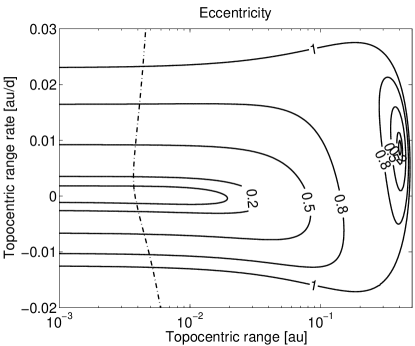
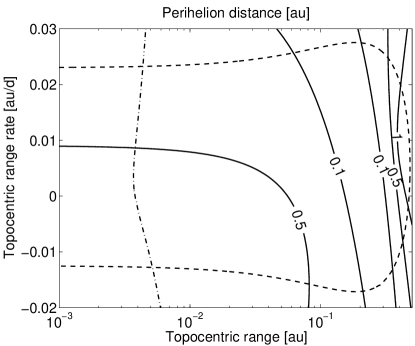
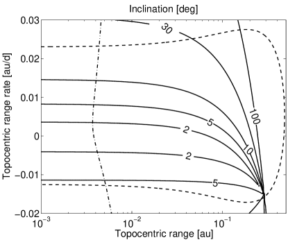
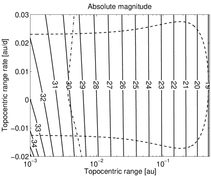
Figure 1 shows the application of systematic ranging to 2014 AA by using the seven astrometric observations obtained by the Catalina Sky Survey prior to impact. The orbital elements are shown as a function of $(\rho,\dot{\rho})$. The dashed curve encloses bounded orbits and corresponds to the admissible region of Milani et al. (2004). The dash-dotted line is for grazing impacts: the region on the left of the curve contains impacting solutions.

3 Probability distribution on the range & range rate space

The raster scan presented in the previous section gives a geometric description of how the orbital configuration depends on the value of topocentric range and range rate. The next step is to assign a probability distribution to this space.

As is common practice, given a set of optical observations we assume that the observation errors $\bm{\nu}$ are normally distributed according to a weight matrix $W$, i.e., their probability density $f_{err}$ is:

$$f_{err}(\bm{\nu})\propto\exp(-0.5\ \bm{\nu}^{T}\,W\,\bm{\nu})\ .$$

It is typical to use a diagonal weight matrix where the individual weights are $1/\sigma^{2}$ ($\sigma$ is the uncertainty in the astrometric positions). Table 1 shows the data weights we currently use for the most productive discovery and follow-up stations. The chosen weights are based on our experience and account for the fact that discovery observations can sometimes be problematic because they are not targeted on the object.

Station	$\sigma_{\alpha,\delta}$	Station	$\sigma_{\alpha,\delta}$	Station	$\sigma_{\alpha,\delta}$
703	1.00′′	G96	0.50′′	F51	0.20′′
950	0.50′′	291	0.70′′	691	0.70′′
568	0.15′′	H01	0.30′′	H21	0.70′′
J04	0.40′′	W84	0.20′′	F65, E10	0.40′′
W85, W86, W87	0.60′′	Q63, Q64, V37	0.80′′	K91, K92, K93	0.80′′

Table 1: Station-specific weighting rules for the most productive discovery and short-term follow-up stations. For all the other stations we use weights at 1^′′.

In principle, it is possible to consider the photometric residuals together with the astrometric ones. However, photometric measurements have a much larger uncertainty than that of the astrometry and can be affected by significant biases (Jurić et al., 2002). Moreover, in case of a magnitude trend, it is hard to tell if the varying luminosity is due to a rapidly changing topocentric distance rather than the asteroid’s rotation. Therefore, we do not use the information obtained from the photometric residuals.

According to Bayesian inversion theory (Muinonen and Bowell, 1993), the posterior probability density function for $(\rho,\dot{\rho})$ is:

$$f_{post}(\rho,\dot{\rho})\propto f_{err}(\bm{\nu}(\rho,\dot{\rho}))\,f_{prior}(\rho,\dot{\rho})\ ,$$

where $f_{prior}$ is a prior distribution on the $(\rho,\dot{\rho})$ space. The selection of $f_{prior}$ is to some extent arbitrary and far from trivial (Jaynes, 1968), and yet can significantly affect the posterior probability distribution, especially for short observation arcs.

Whatever the choice of $f_{prior}$, we always add a crude constraint from the population model by setting $f_{prior}=0$ for hyperbolic orbits, flagging objects where the astrometric errors favor an unbounded orbit.

3.1 Jeffreys’ prior

A mathematically sound choice is Jeffreys’ prior (Granvik et al., 2009):

$$f_{prior}(\rho,\dot{\rho})=\sqrt{\det\left(\frac{\partial\bm{\nu}}{\partial(\rho,\dot{\rho})}^{T}\ W\ \frac{\partial\bm{\nu}}{\partial(\rho,\dot{\rho})}\right)}\ .$$ (2)

Note that the partials are the total derivatives of $\bm{\nu}$ with respect to $(\rho,\dot{\rho})$, which means that they account for the fact that the best-fit attributable ${\cal A}$ changes as a function of $(\rho,\dot{\rho})$.

Among other things, Jeffreys’ prior secures the invariance of the probability distribution when changing variables. However, since there is more sensitivity of the residuals for small topocentric distances, Jeffreys’ prior tends to favor orbital configurations where the object is close to the observer, e.g., see the examples of 2015 CV and 2015 BU₉₂ in Sec. 6.

3.2 Prior based on population model

As already discussed by Virtanen et al. (2001), the prior could be based on the known asteroid population. Even better, one could use an orbit and size population model where the known population is extrapolated to remove survey selection effects and to reach completeness up to a given apparent magnitude. One such model is the Pan-STARRS Synthetic Solar System Model (Grav et al., 2011), and new population models are expected in the future (Granvik et al., 2014). From the Grav et al. (2011) model we derived a probability density $f_{pop}(q,e,i,H)$ for perihelion distance $q$, eccentricity $e$, inclination $i$, and absolute magnitude $H$. A more refined approach would be to remove the known population from the population model.

Mapping $f_{pop}$ to the best fitting orbits in the $(\rho,\dot{\rho})$ plane is quite complicated. Therefore, to compute such a prior we iteratively apply Bayesian inversion theory, i.e., the prior is computed as posterior $f_{post}^{\prime}$ of another prior $f_{prior}^{\prime}$:

$$f_{prior}(\rho,\dot{\rho})=f_{post}^{\prime}(\rho,\dot{\rho})\propto f_{prior}^{\prime}(\rho,\dot{\rho})f_{pop}(q(\rho,\dot{\rho}),e(\rho,\dot{\rho}),i(\rho,\dot{\rho}),H(\rho,\dot{\rho}))\,.$$

At this point we select $f_{prior}^{\prime}$ using simple geometric considerations. By assuming that the Cartesian space of position and velocity is uniformly filled, we have that $\rho^{3}$ and $\dot{\rho}$ are uniformly distributed. Hence, $f_{prior}^{\prime}(\rho,\dot{\rho})\propto\rho^{2}$.

3.3 Uniform prior

A common choice for $f_{prior}$ is a uniform distribution. For instance, such a prior is used by Virtanen et al. (2001) and Oszkiewicz et al. (2009). Interestingly, it is possible to approximately obtain a prior distribution from the population model if we only consider the size distribution $f_{size}(H)$, i.e., $f_{prior}=\rho^{2}f_{size}(H)$.

For near-Earth asteroids the cumulative size distribution is expected to follow a power law $f_{size}(H)\propto 10^{\eta H}$, with $\eta$ somewhere between 0.35 and 0.47 (Bottke et al., 2002; Harris, 2002; Stuart and Binzel, 2004). For a given visual magnitude $V$, we have that $f_{size}(H)\propto\rho^{-5\eta}$ (Bowell et al., 1989) and therefore $f_{prior}=\rho^{2-5\eta}$. According to the range of possible values for $\eta$, this prior corresponds to a power law with exponent between $-0.35$ and $0.25$, which is compatible with a uniform distribution.

Though a uniform distribution might appear overly simplistic, we have found that this it does a good job of identifying potential impactors (e.g., see Sec. 6) and distinguishing interesting objects from more common ones, such as main belt asteroids.

4 Impact probability computation

For each grid point, as a result of the constrained least squares fit to the observations, we obtain not only a best fit value ${\cal A}_{ij}$ of the attributable, but also the corresponding uncertainty expressed by a covariance matrix $\Gamma_{{\cal A}_{ij}}$. This uncertainty is easily mapped to the orbital element space and therefore allows us to compute the probability $p_{ij}$ of an Earth impact for that orbit. Since for a fixed grid point the orbital uncertainty is small and the horizon for impacts is of the order of weeks, we compute the impact probability with a linear approach (Milani et al., 2002; Farnocchia et al., 2015).

Given $f_{post}$ we can assign each grid point a weight $w_{ij}\propto f_{post}(\rho_{i},\dot{\rho}_{j})$, where $\sum w_{ij}=1$. Then, the impact probability can be easily computed as

$$P=\sum w_{ij}p_{ij}.$$

5 Generation of Monte Carlo orbital samples

To better visualize the orbital distribution, it is convenient to generate Monte Carlo orbital samples distributed according to the probability distribution computed above. The following procedure can be used to achieve this goal:

(a)

Randomly draw $\rho_{k}$ according to a uniform distribution between the minimum and maximum values of $\rho$ on the grid;

(b)

Randomly draw $\dot{\rho}_{k}$ according to a uniform distribution between the minimum and maximum values of $\dot{\rho}$ on the grid;

(c)

Randomly draw a value $\gamma$ according to a uniform distribution between 0 and the maximum of $f_{post}$ on the grid;

(d)

Compute a best-fit attributable ${\cal A}_{k}$ for $(\rho,\dot{\rho})=(\rho_{k},\dot{\rho}_{k})$;

(e)

If $f_{post}(\rho_{k},\dot{\rho}_{k})\geq\gamma$ go to (f), otherwise start again from (a);

(f)

Add normally distributed noise to ${\cal A}_{k}$ according to the covariance $\Gamma_{{\cal A}_{k}}$ and add $({\cal A}_{k},\rho_{k},\dot{\rho}_{k})$ to the sequence of orbital samples.

6 Examples

We want to test the algorithm presented in the previous sections on real cases. On one hand it is important that systematic ranging provides an early detection of impacting asteroids. On the other hand we need to avoid generating too many warnings for objects that might be very far from Earth. Thus, we show examples of impactors as well as main belt asteroids. Table 2 summarizes the results for the examples discussed in more detail in the following subsections.

Object	Number	Arc	Weights	Impact probability
	of obs	length		Jeffreys	Uniform	Population
2008 TC3	4	43 min	0.5′′	$6.3\times 10^{-1}$	$4.4\times 10^{-2}$	$2.4\times 10^{-2}$
2008 TC3	4	43 min	1.0′′	$6.7\times 10^{-1}$	$3.7\times 10^{-3}$	$3.5\times 10^{-3}$
2008 TC3	7	99 min	0.5′′	$1.0$	$1.0$	$1.0$
2008 TC3	7	99 min	1.0′′	$9.7\times 10^{-1}$	$9.8\times 10^{-1}$	$9.6\times 10^{-1}$
2014 AA	3	28 min	0.5′′	$8.1\times 10^{-1}$	$2.9\times 10^{-2}$	$3.1\times 10^{-2}$
2014 AA	3	28 min	1.0′′	$8.4\times 10^{-1}$	$3.3\times 10^{-3}$	$8.4\times 10^{-3}$
2014 AA	7	69 min	0.5′′	$1.0$	$1.0$	$1.0$
2014 AA	7	69 min	1.0′′	$9.9\times 10^{-1}$	$9.6\times 10^{-1}$	$9.0\times 10^{-1}$
Hayabusa	3	7 min	1.0′′	$9.4\times 10^{-1}$	$2.7\times 10^{-3}$	$2.0\times 10^{-3}$
Hayabusa	6	34 min	1.0′′	$2.4\times 10^{-1}$	$1.7\times 10^{-1}$	$2.2\times 10^{-2}$
Hayabusa 2	3	43 min	0.2′′	$2.8\times 10^{-1}$	$3.6\times 10^{-1}$	$4.2\times 10^{-1}$
Hayabusa 2	3	43 min	0.5′′	$3.6\times 10^{-1}$	$3.3\times 10^{-2}$	$7.2\times 10^{-2}$
Hayabusa 2	6	26 h	0.2′′	$2.4\times 10^{-13}$	$2.3\times 10^{-13}$	$2.2\times 10^{-13}$
Hayabusa 2	6	26 h	0.5′′	$1.9\times 10^{-3}$	$1.9\times 10^{-3}$	$1.8\times 10^{-3}$
2004 AS1	4	71 min	1.0′′	$2.2\times 10^{-1}$	$1.2\times 10^{-1}$	$7.8\times 10^{-2}$
2004 AS1	4	71 min	1.5′′	$1.2\times 10^{-1}$	$1.3\times 10^{-2}$	$1.1\times 10^{-2}$
2004 FU162	4	44 min	1.0′′	$3.6\times 10^{-1}$	$7.3\times 10^{-3}$	$8.7\times 10^{-4}$
2004 FU162	4	44 min	1.5′′	$5.0\times 10^{-1}$	$1.3\times 10^{-2}$	$1.0\times 10^{-3}$
2015 CV	4	34 min	0.5′′	$8.5\times 10^{-3}$	$4.7\times 10^{-6}$	$9.9\times 10^{-7}$
2015 CV	4	34 min	1.0′′	$1.7\times 10^{-1}$	$1.5\times 10^{-4}$	$4.6\times 10^{-5}$
2015 BU92	3	36 min	0.5′′	$1.7\times 10^{-1}$	$7.2\times 10^{-5}$	$3.5\times 10^{-10}$
2015 BU92	3	36 min	1.0′′	$4.8\times 10^{-1}$	$4.0\times 10^{-4}$	$8.5\times 10^{-8}$

Table 2: Impact probabilities for the examples considered in Sec. 6 for different choices of $f_{prior}$, different number of tracklets, and different data weights.

6.1 2008 TC₃

Figure 2: Normalized RMS as a function of $(\rho,\dot{\rho})$ for 2008 TC₃. Left panel is for the first tracklet (four observations over 43 min), right panel is for the first two tracklets (total of seven observations over 99 min). Astrometric weights are at 0.5^′′. The dashed curve corresponds to parabolic heliocentric orbits and the dash-dotted line to grazing impacts.

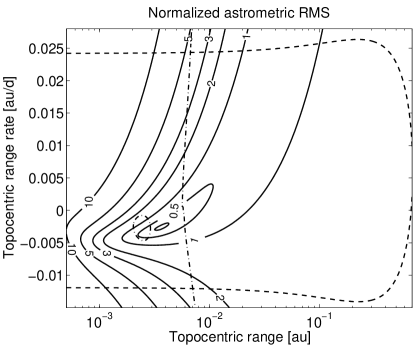
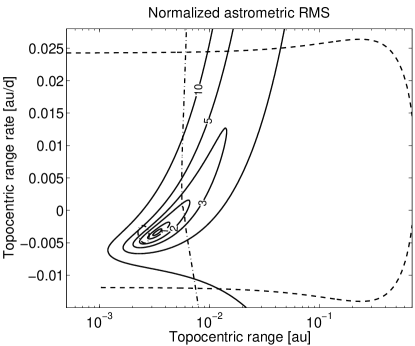
As already discussed in the introduction, 2008 TC₃ was the first asteroid discovered prior to impact. This object was first spotted and promptly followed up by R. A. Kowalski at the Mt. Lemmon observatory. In the 20 hours between discovery and impact hundreds of astrometric observations were reported to the Minor Planet Center. These observations allowed the calculation of a least squares orbit and the prediction of the impact. How would systematic ranging have performed with the first observations of 2008 TC₃?

The left panel of Fig. 2 shows the normalized RMS, i.e., the square root of the target function $Q$ in Eq. (1), as a function of $(\rho,\dot{\rho})$ by using the first tracklet of four observations obtained by Kowalski. The nonlinearity of the orbit determination problem is evident from the level curves of the RMS, which clearly suggest that 2008 TC₃ could be on an impact trajectory. As a matter of fact, the corresponding impact probability, computed as described in Sec. 4, is already significant with the first four observations (Table 2). With our defaults data weights at 0.5^′′, the impact probability is few percents when using a uniform prior or one based on the population model, and $\sim$60% when using Jeffreys’ prior. With more conservative weights at 1^′′ Jeffreys’ prior leads to a $\sim$70% impact probability, while the uniform and population prior result in a probability of few in a thousand.

With the addition of Kowalski’s second tracklet, three additional observations, the orbit becomes much better constrained by the observation residuals (see right panel of Fig. 2). The impact is now almost certain, especially with 0.5^′′ weights.

Figure 3: Potential impact locations for 2008 TC₃ based on the first two tracklets of data.

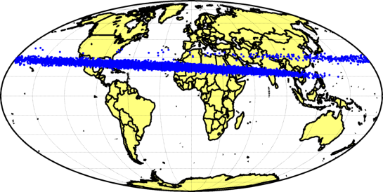
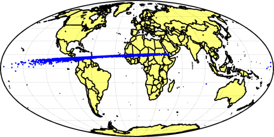
By using the first two tracklets of data and adopting a uniform prior, we also generated Monte Carlo samples to find potential impact locations, as shown in Fig. 3. As expectable, the region of possible impact location contains the Sudan desert where 2008 TC₃ actually ended its journey (Jenniskens et al., 2009).

6.2 2014 AA

Though 2014 AA was not extensively followed up after discovery, there are several similarities with 2008 TC₃. In particular, 2014 AA was also discovered about 20 hours before impact by R. A. Kowalski at the Mt. Lemmon observatory.

Figure 4: Normalized RMS as a function of $(\rho,\dot{\rho})$ for 2014 AA. Left panel is for the first tracklet (three observations over 28 min), right panel is for the first two tracklets (total of seven observations over 69 min). Astrometric weights are at 0.5^′′. The dashed curve corresponds to parabolic heliocentric orbits and the dash-dotted line to grazing impacts.

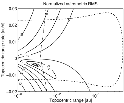
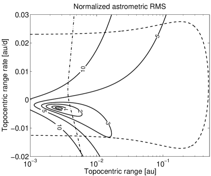
Figure 4 shows the normalized RMS for 2014 AA as a function of $(\rho,\dot{\rho})$ by using the first tracklet of data (three observations) or the full available dataset (seven observations). Again, the RMS curves clearly indicate that an impact is possible. Systematic ranging immediately recognizes the potential impact from the first tracklet and make the impact almost certain when the second tracklet is added. Table 2 reports the computed impact probabilities, which are similar to those computed for 2008 TC₃,.

Figure 5: Potential impact locations for 2014 AA based on all available data, i.e., seven observations.

The impact locations (see Fig. 5) found by using the seven available observations and adopting a uniform prior are statistically consistent with the detection by the infrasound component of the International Monitoring System (IMS) operated by the Comprehensive Nuclear Test Ban Treaty Organization (CTBTO), which places the impact location in the Atlantic Ocean at a latitude of about 15^∘ N and a longitude of about 43^∘ W (Chesley et al., 2015; Brown, 2014).

6.3 Hayabusa & Hayabusa 2

Because of the low number of actual impactors we can use as a validation, we tested our algorithm on Hayabusa and Hayabusa 2 (Kawaguchi et al., 2008).

Figure 6: Normalized RMS as a function of $(\rho,\dot{\rho})$ for Hayabusa. Left panel is for the first tracklet (three observations over 7 min), right panel is for the first two tracklets (total of seven observations over 34 min). Astrometric weights are at 1.0^′′. The dashed curve corresponds to parabolic heliocentric orbits and the dash-dotted line to grazing impacts.

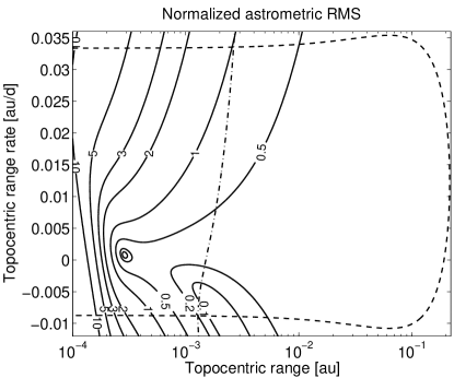
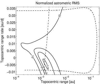
The reentry of Hayabusa took place on 2010 June 13. Yamaguchi et al. (2011) report ground-based observations acquired during the reentry phase, which ended with a landing in the South Australia outback. We used these observations for applying systematic ranging technique to Hayabusa. Figure 6 shows the normalized RMS as a function of $(\rho,\dot{\rho})$ by using the first tracklet of data (three observations) or the full available dataset (six observations). Table 2 gives the impact probability as a function of the number of observations. With a uniform prior the initial impact probability is $2.7\times 10^{-3}$ and increases to 17% with the second tracklet. With the population-based prior the initial impact probability is $2.0\times 10^{-3}$ and increases to 2% with the second tracklet. On the other hand, with the use of Jefrreys’ prior we immediately have a 94% impact probability that decreases to 24% with the second tracklet. This counterintuitive behavior is due to the presence of two local RMS minima with the first tracklet, one of which clearly corresponds to an impact and is ruled out by the second tracklet.

Hayabusa 2 was launched on 2014 December 3. After launch Hayabusa 2 was initially put on a low Earth parking orbit, until a maneuver moved it onto a ballistic trajectory leaving the Earth. On its way out, on 2014 December 6, Hayabusa 2 happend to be in the field of view of the Pan-STARRS PS1 survey (Wainscoat et al., 2014), which collected three observations of the spacecraft over 43 min. The corresponding astrometry was submitted to the Minor Planet Center, which, since the observations were not recognized as belonging to the Hayabusa 2 spacecraft, put the object on the NEO Confirmation Page with the temporary designation P10gJfF. The following day, 2014 December 7, Pan-STARRS obtained three additional observations from which it became clear that the object was Hayabusa 2. Table 2 shows how systematic ranging recognizes Hayabusa 2 as potential impactor from the first three observations with an impact probability probability of few to ten percents, depending on the data weights and the prior used. Then, the subsequent observations better constrain the orbit and lower the impact probability since the ballistic trajectory does not correspond to an impact but to the post-injection escape orbit.

6.4 2004 AS₁

Asteroid 2004 AS₁ was discovered by LINEAR (Stokes et al., 2000) on 2004 January 13 (Blythe et al., 2004a). The four discovery observations span 71 min and show an unusually high curvature thus suggesting that 2004 AS₁ was close to the Earth and that an impact was possible. Follow-up observations later showed that the object was much farther than originally thought, thus ruling out any impact, and that the observed curvature was due to large astrometric errors in the discovery observations.

Virtanen and Muinonen (2006) employed the statistical ranging technique (Virtanen et al., 2001) to analyze the 2004 AS₁ case. They found an 18% impact probability with 1.0^′′ weights and concluded that such a large impact probability was mostly due to the poor quality of the discovery night observations.

The left panel of Fig. 7 shows the application of systematic ranging to 2004 AS₁. The astrometric observations are weighted at 1.0^′′. The RMS favors an impact solution while the true solution (marked with a cross) correspond to larger astrometric errors. The impact probabilities computed for the different choices of the prior distribution are of the order of 10%, see Table 2. Decreasing the weights at 1.5^′′ gives significantly lower probabilities for the uniform and population-based priors, while with Jefrreys’ prior we still have a 12% impact probability.

Figure 7: Normalized RMS as a function of $(\rho,\dot{\rho})$ for 2004 AS₁ (left panel) and 2004 FU₁₆₂ (right panel). Astrometric weights are at 1.0^′′. The dashed curve corresponds to parabolic heliocentric orbits and the dash-dotted line to grazing impacts. For 2004 AS₁ the cross marks the true solution.

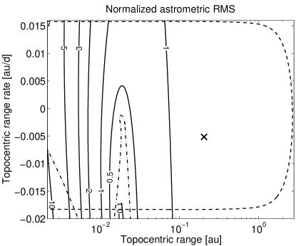
As shown by Table 3, we computed the $p$-value of the true solution, i.e., the fraction of less likely orbital solutions, for the different choices of the prior and different data weights. Jeffreys’ prior produces very small $p$-values thus indicating that the true solution is deemed as extremely unlikely by the computed probability distribution. For the uniform distribution we have 3% $p$-value with 1^′′ weights, which is due to the large errors in the astrometric observations. As a matter of fact, relaxing the weights increases the $p$-value to 22%. On the other hand, the population-based prior compensates for the large astrometric errors since impacting solutions with low RMS are less likely in the population model than non-impacting solutions with a higher RMS. The $p$-values are 13.6% and 38.7% depending on the data weights.

Object	Weights	$p$-value
		Jeffreys	Uniform	Population
2004 AS1	1.0′′	$3.1\times 10^{-5}$	$2.6\times 10^{-2}$	$1.4\times 10^{-1}$
2004 AS1	1.5′′	$4.0\times 10^{-4}$	$2.2\times 10^{-1}$	$3.9\times 10^{-1}$
2015 CV	0.5′′	$5.0\times 10^{-5}$	$4.9\times 10^{-1}$	$4.2\times 10^{-1}$
2015 CV	1.0′′	$1.3\times 10^{-5}$	$4.9\times 10^{-1}$	$4.2\times 10^{-1}$
2015 BU92	0.5′′	$1.1\times 10^{-5}$	$9.1\times 10^{-1}$	$8.8\times 10^{-1}$
2015 BU92	1.0′′	$2.3\times 10^{-6}$	$9.1\times 10^{-1}$	$8.9\times 10^{-1}$

Table 3: $p$-values for some of the examples considered in Sec. 6 for different choices of $f_{prior}$ and different data weights.

The conclusion fpr 2004 AS₁ is that the discovery tracklet, weighted at 1^′′, yields impact probabilities $\sim 10\%$ even as the trueth is compatible with the data at the 3–14% level. This outcome is a manifestation of the large astrometric errors in the data.

6.5 2004 FU₁₆₂

Asteroid 2004 FU₁₆₂ was also discovered by LINEAR on 2004 March 31 (Blythe et al., 2004b). Chesley (2005) first analyzed this object and estimated that there was a 0.3% probability of an impact and that the object was likely to pass within 10 Earth radii.

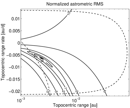
The right panel of Fig. 7 shows our implementation of systematic ranging, while Table 2 reports the impact probabilities for different weights and prior distributions. Again, Jeffreys’ prior results in very high impact probabilities while the population-based prior gives the lowest impact chances. For 1^′′ weights the impact probability is 0.7% – 0.9% with the uniform and the population based priors. An Earth encounter within 10 Earth radii is assured with all three priors, thus confirming the findings of Chesley (2005).

6.6 2015 CV & 2015 BU₉₂

Figure 8: Normalized RMS as a function of $(\rho,\dot{\rho})$ for 2015 CV (left panel) and 2015 BU₉₂ (right panel). Astrometric weights are at 0.5^′′. The dashed curve corresponds to parabolic heliocentric orbits and the dash-dotted line to grazing impacts. Crosses mark the true solutions.

The previous examples show how systematic ranging is capable of quickly identifying actual and potential impactors. However, there is the risk of having significant impact probabilities ($10^{-3}$ or higher) for a large number of objects, which would make it difficult to distinguish interesting objects from less remarkable ones. Here we show the example of two main belt objects that were recently posted on the NEO Confirmation Page when the initial observations were compatible with an NEO orbit: 2015 CV and 2015 BU₉₂.

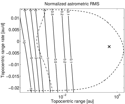
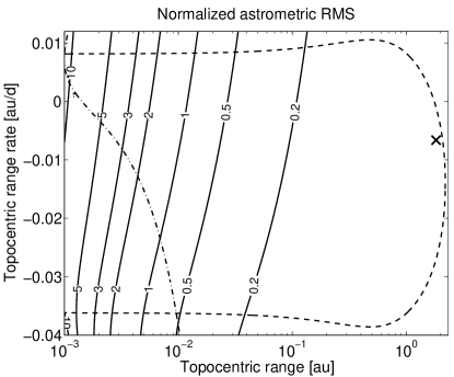
2015 CV was discovered by the Catalina Sky survey, Mt. Lemmon station, on 2015 February 10, while 2015 BU₉₂ was discovered by Spacewatch (McMillan, 2000), Kitt Peak observatory, on 2015 January 16 (Bressi and Tubbiolo, 2015). Figure 8 shows the application of systematic ranging to these two asteroids. For both objects the region with reasonable astrometric errors extends from impacting solutions to more than 1 au from the observer.

As shown by Table 2 and Table 3, in both cases Jeffreys’ prior provides significant impact probabilities and extremely low $p$-values for the true solutions. In fact, Jeffreys’ prior is proportional to the partials of the astrometric residuals and the residuals do not change much for large topocentric distances while they are very sensitive when the object is close to the observer. Therefore, Jeffreys’ prior tends to favor small topocentric distances even if the astrometric errors are larger. On the other hand the uniform and the population-based priors give much more reasonable probabilities and $p$-values.

7 Discussion and future work

Small asteroids are expected to strike the Earth on a regular basis. For instance, according to Brown et al. (2002) impacts with 10 m sized objects take place every few years. Since such small asteroids are likely to be observed, if at all, only shortly before impact, it is important to be capable of an early recognition of hazardous objects.

The shortness of the observation arcs typically available for these objects leads to critical degeneracies in the orbit estimation process and limits the applicability of the standard impact monitoring systems (Milani et al., 2005). The systematic ranging technique presented in this paper relies on Bayesian inversion theory, which overcomes these degeneracies and results in a posterior distribution on the orbit phase space.

A critical point is the choice of a prior distribution for the poorly constrained space of topocentric range and range rate. This choice is far from trivial and indeed is somewhat arbitrary. We analyzed three options: Jeffreys’ prior, a uniform prior, and a prior distribution based on the asteroid population model.

Jeffreys’ prior does a good job at assigning high impact probabilities to actual impactors. However, this prior produces high impact probabilities also for less remarkable objects such as main belt asteroids. The reason for this behavior is that Jeffreys’ prior favors regions in the phase space that are closer to the observer. As a matter of fact, Jeffreys’ prior is proportional to the partials of the residuals with respect to topocentric range and range rate, which are large for small topocentric distances and vanish at large distances. Moreover, in the non-impacting examples we analyzed we found that the true solution was often deemed as extremely unlikely by the posterior distribution obtained starting from Jeffreys’ prior. Therefore, we avoid the use of Jeffreys’ prior for systematic ranging.

The prior based on the asteroid orbit and size distribution represents the highest fidelity and most complex choice. However, it is worth pointing out that a population model is necessarily limited by the finite number of samples and is therefore affected by Poisson statistics errors. In particular, small impactors might have peculiar orbits that are deemed unlikely by the model, which could be too much of a risk when the main goal is to identify potential impactors.

A uniform distribution represents a compromise between simplicity and reliability. Though the corresponding posterior distribution and impact probabilities are not as rigorous as the one resulting from the population-based prior, we found that a uniform prior is effective at flagging potential impactors and discriminating between hazardous asteroids and more distant ones, which is the most important task to be achieved by systematic ranging. Another advantage of the uniform prior is that it has little prejudice on the actual orbit.

To complement the standard impact monitoring performed by JPL’s Sentry and the University of Pisa’s NEODyS, we have implemented an automated system to continually analyze the objects on the Minor Planet Center’s NEO Confirmation Page with systematic ranging. This system quickly computes an impact probability to identify potential impactors and notifies us of interesting results. In such cases, we have communicated with discoverers and other observers to solicitate a quality control of the reported astrometry and for acquiring follow-up observations, which are necessary to decrease the orbital uncertainties and conclusively determine if the impact is going to take place. The examples of 2008 TC₃ and 2014 AA, i.e., the only two asteroids discovered before striking the Earth, suggest that objects with an impact probability above $10^{-3}$ should be prioritized for prompt follow-up. In recent experience this happens a few to several times a month.

Among the possible additional applications of the systematic ranging technique presented in this paper, one could be the identification potential radar targets or mission-accessible targets, e.g., for the NASA’s Asteroid Redirect Mission (Abell et al., 2014).

References

- Abell et al. (2014) Abell, P., Gates, M., Johnson, L., Chodas, P., Brophy, J., Mazanek, D., Muirhead, B. 2014. NASA’s Asteroid Redirect Mission: Overview and Status. 40th COSPAR Scientific Assembly 40, 17.
- Blythe et al. (2004a) Blythe, M, Shelly, F., Bezpalko, M., et al. 2004. 2004 AS1. Minor Planet Electronic Circulars 2004-A56.
- Blythe et al. (2004b) Blythe, M, Shelly, F., Bezpalko, M., et al. 2004. 2004 FU162. Minor Planet Electronic Circulars 2004-Q22.
- Bottke et al. (2002) Bottke, W. F., Morbidelli, A., Jedicke, R., Petit, J.-M., Levison, H. F., Michel, P., Metcalfe, T. S. 2002. Debiased Orbital and Absolute Magnitude Distribution of the Near-Earth Objects. Icarus 156, 399-433.
- Bowell et al. (1989) Bowell, E., Hapke, B., Domingue, D., Lumme, K., Peltoniemi, J., Harris, A. W. 1989. Application of photometric models to asteroids. Asteroids II 524-556.
- Bressi and Tubbiolo (2015) Bressi, T. H., Tubbiolo, A. F., 2015. 2015 BU92. Minor Planet Electronic Circulars 2015-B95.
- Brown et al. (2002) Brown, P., Spalding, R. E., ReVelle, D. O., Tagliaferri, E., Worden, S. P. 2002. The flux of small near-Earth objects colliding with the Earth. Nature 420, 294-296.
- Brown (2014) Brown, P. 2014. Using the international monitoring system of seismic, infrasound, and hydroacoustic sensors for global airburst detection. Asteroids, Comets, Meteors 2014 63.
- Chesley (2005) Chesley, S. R. 2005. Very short arc orbit determination: the case of asteroid 2004 FU162. IAU Colloq. 197: Dynamics of Populations of Planetary Systems 255-258.
- Chesley et al. (2015) Chesley, S. R., Farnocchia, D., Brown, P., Chodas, P. W. 2015. Orbit Estimation for Late Warning Asteroid Impacts: The Case of 2014 AA. IEEE Aerospace Conference, #2.1202.
- Farnocchia et al. (2015) Farnocchia, D., Chesley, S. R., Milani, A., Gronchi, G. F., Chodas, P. W. 2015. Orbits, long-term predictions, impact monitoring. Asteroids IV, In press.
- Granvik et al. (2009) Granvik, M., Virtanen, J., Oszkiewicz, D., Muinonen, K. 2009. OpenOrb: Open-source asteroid orbit computation software including statistical ranging. Meteoritics and Planetary Science 44, 1853-1861.
- Granvik et al. (2014) Granvik, M., Morbidelli, A., Jecicke, R., et al. 2014. Unbiased dynamical and physical characteristics of the near-Earth-object population. Asteroids, Comets, Meteors 2014 180.
- Grav et al. (2011) Grav, T., Jedicke, R., Denneau, L., Chesley, S., Holman, M. J., Spahr, T. B. 2011. The Pan-STARRS Synthetic Solar System Model: A Tool for Testing and Efficiency Determination of the Moving Object Processing System. Publications of the Astronomical Society of the Pacific 123, 423-447.
- Harris (2002) Harris, A. W. 2002. A New Estimate of the Population of Small NEAs. Bulletin of the American Astronomical Society 34, 835.
- Jaynes (1968) Janyes, E. T. 1968. Priori Probabilities. IEEE Transactions On Systems Science and Cybernetics 4, 227-241.
- Jenniskens et al. (2009) Jenniskens, P., Shaddad, M. H., Numan, D., et al. 2009. The impact and recovery of asteroid 2008 TC3. Nature 458, 485-488.
- Jurić et al. (2002) Jurić, M., Ivezić, Ž., Lupton, R. H., et al. 2002. Comparison of Positions and Magnitudes of Asteroids Observed in the Sloan Digital Sky Survey with Those Predicted for Known Asteroids. The Astronomical Journal 124, 1776-1787.
- Kawaguchi et al. (2008) Kawaguchi, J., Fujiwara, A., Uesugi, T. 2008. Hayabusa—Its technology and science accomplishment summary and Hayabusa-2. Acta Astronautica 62, 639-647.
- Kowalski et al. (2008) Kowalski, R. A., Beshore, E. C., Boattini, A., et al. 2008. 2008 TC3. Minor Planet Electronic Circulars 2008-T50.
- Kowalski et al. (2014) Kowalski, R. A., Boattini, A., Christesen, E. J., et al. 2014. 2014 AA. Minor Planet Electronic Circulars 2014-A02.
- Kozubal et al. (2011) Kozubal, M. J., Gasdia, F. W., Dantowitz, R. F., Scheirich, P., Harris, A. W. 2011. Photometric observations of Earth-impacting asteroid 2008 TC3. Meteoritics and Planetary Science 46, 534-542.
- Kubica et al. (2007) Kubica, J., Denneau, L., Grav, T., Heasley, J., Jedicke, R., Masiero, J., Milani, A., Moore, A., Tholen, D., Wainscoat, R. J. 2007. Efficient intra- and inter-night linking of asteroid detections using kd-trees. Icarus 189, 151-168.
- Larson et al. (1998) Larson, S., Brownlee, J., Hergenrother, C., Spahr, T. 1998. The Catalina Sky Survey for NEOs. Bulletin of the American Astronomical Society 30, 1037.
- McMillan (2000) McMillan, R. S. 2000. Spacewatch Survey of the Solar System. NASA STI/Recon Technical Report N 1, 18998.
- Milani et al. (2002) Milani, A., Chesley, S. R., Chodas, P. W., Valsecchi, G. B. 2002. Asteroid Close Approaches: Analysis and Potential Impact Detection. Asteroids III 55-69.
- Milani et al. (2004) Milani, A., Gronchi, G. F., Vitturi, M. D., Knežević, Z. 2004. Orbit determination with very short arcs. I admissible regions. Celestial Mechanics and Dynamical Astronomy 90, 57-85.
- Milani et al. (2005) Milani, A., Chesley, S. R., Sansaturio, M. E., Tommei, G., Valsecchi, G. B. 2005. Nonlinear impact monitoring: line of variation searches for impactors. Icarus 173, 362-384.
- Milani and Knežević (2005) Milani, A., Knežević, Z. 2005. From Astrometry to Celestial Mechanics: Orbit Determination with Very Short Arcs. Celestial Mechanics and Dynamical Astronomy 92, 1-18.
- Milani and Gronchi (2010) Milani, A., Gronchi, G. F. 2010. Theory of Orbit Determination. Cambridge University Press, Cambridge, UK, 2010.
- Muinonen and Bowell (1993) Muinonen, K., Bowell, E. 1993. Asteroid orbit determination using Bayesian probabilities. Icarus 104, 255-279.
- Oszkiewicz et al. (2009) Oszkiewicz, D., Muinonen, K., Virtanen, J., Granvik, M. 2009. Asteroid orbital ranging using Markov-Chain Monte Carlo. Meteoritics and Planetary Science 44, 1897-1904.
- Scheirich et al. (2010) Scheirich, P., et al. 2010. The shape and rotation of asteroid 2008 TC3. Meteoritics and Planetary Science 45, 1804-1811.
- Stokes et al. (2000) Stokes, G. H., Evans, J. B., Viggh, H. E. M., Shelly, F. C., Pearce, E. C. 2000. Lincoln Near-Earth Asteroid Program (LINEAR). Icarus 148, 21-28.
- Stuart and Binzel (2004) Stuart, J. S., Binzel, R. P. 2004. Bias-corrected population, size distribution, and impact hazard for the near-Earth objects. Icarus 170, 295-311.
- Virtanen et al. (2001) Virtanen, J., Muinonen, K., Bowell, E. 2001. Statistical Ranging of Asteroid Orbits. Icarus 154, 412-431.
- Virtanen and Muinonen (2006) Virtanen, J., Muinonen, K. 2006. Time evolution of orbital uncertainties for the impactor candidate 2004 AS1. Icarus 184, 289-301.
- Wainscoat et al. (2014) Wainscoat, R., Veres, P., Bolin, B., Denneau, L., Jedicke, R., Chastel, S., Micheli, M. 2014. The Pan-STARRS search for near-Earth objects. Asteroids, Comets, Meteors 2014 574.
- Yamaguchi et al. (2011) Yamaguchi, T., Yoshikawa, M., Yagi, M., Tholen, D. J. 2011. Entry Dispersion Analysis for the HAYABUSA Spacecraft using Ground-Based Optical Observation. Publications of the Astronomical Society of Japan 63, 979-985.