Solutions of Laplace’s equation with simple boundary conditions, and their applications for capacitors with multiple symmetries

Abstract

We find solutions of Laplace’s equation with specific boundary conditions (in which such solutions take either the value zero or unity in each surface) using a generic curvilinear system of coordinates. Such purely geometrical solutions (that we shall call Basic Harmonic Functions BHF’s) are utilized to obtain a more general class of solutions for Laplace’s equation, in which the functions take arbitrary constant values on the boundaries. On the other hand, the BHF’s are also used to obtain the capacitance of many electrostatic configurations of conductors. This method of finding solutions of Laplace’s equation and capacitances with multiple symmetries is particularly simple, owing to the fact that the method of separation of variables becomes much simpler under the boundary conditions that lead to the BHF’s. Examples of application in complex symmetries are given. Then, configurations of succesive embedding of conductors are also examined. In addition, expressions for electric fields between two conductors and charge densities on their surfaces are obtained in terms of generalized curvilinear coordinates. It worths remarking that it is plausible to extrapolate the present method to other linear homogeneous differential equations.

Keywords: Laplace’s equation, curvilinear coordinates, capacitance, harmonic functions, separation of variables.

Introduction

Solutions of Laplace’s equation, usually called Harmonic Functions (HF’s) are very important in many branches of Physics and Engineering such as electrostatics, gravitation, hydrodynamics and thermodynamics[1, 2]. Therefore, considerable effort has been done in solving Laplace’s equation [28]-[35] in a variety of geometries and boundary conditions. On the other hand, the capacitance of electrostatic conductors is a very important quantity since capacitors are present in many electric and electronic devices [12]-[14]. Thus, many studies of its general properties [2]-[11], and calculations of coefficients of capacitance for many geometric configurations [15]-[28] have been carried out.

The first goal in this paper is to show a simple method to solve Laplace’s equation for configurations of volumes with certain symmetries, when the HF’s acquire values of either zero or unity in each surface that provides the boundary conditions. The solutions of Laplace’s equation under these specific boundary conditions will be called Basic Harmonic Functions (BHF’s). We shall see that the form of these boundary conditions leads to very easy solutions via separation of variables. Besides, the solutions will be written in terms of a generic system of curvilinear coordinates that can be adjusted for many symmetries. It is remarkable that the BHF’s depends exclusively on the geometry, and not on the physical problem involved.

The determination of the BHF’s under a given geometry will be applied in two scenarios: $\mathbf{(a)}$ The generation of a more general class of solutions in which the HF’s take arbitrary constant values on the surfaces that determine the volume. $\mathbf{(b)\ }$The calculation of the coefficients of capacitance when the surfaces that form the volume are covered with electrostatic conductors. Once again, both types of solutions are given in a generic form in terms of appropriate generalized systems of coordinates.

The paper is distributed as follows: In section 1, we solve Laplace’s equation in generalized geometrical configurations to obtain the BHF’s, by using a generic system of curvilinear coordinates. As a matter of illustration of the method, we obtain the BHF’s for the cases of two concentric spheres and two concentric cylinders. Then, from the BHF’s obtained in Sec. 1 and appealing to the linearity of Laplace’s equation, we construct in Sec. 2 a more general class of solutions in which HF’s acquire arbitrary constant values on the surfaces. On the other hand, in section 3, we use the general expressions for the BHF’s in generalized curvilinear coordinates, in order to obtain the corresponding generalized formulas for the coefficients of capacitance. The capacitance coefficients for the cases of two concentric spheres and two concentric cylinders are obtained for illustration. Then, section 4 shows calculations of BHF’s and capacitances for more complex geometries in which our formulation acquires all its power. Moreover, in appendix A, we obtain the electric field between two conductors as well as charge densities on their surfaces in terms of curvilinear coordinates, while in appendix B, formulas for the coefficients of capacitance are extended to the case in which we have a configuration of succesively embedded conductors. Appendix C provides some relations between curvilinear coordinates and geometrical factors. Finally, section 5 contains our conclusions.

1 Laplace’s equation and systems of orthogonal curvilinear coordinates

Laplace’s equation given by

$$\nabla^{2}f=0$$ (1)

has solutions that depend on the boundary conditions. It is desirable to use a system of coordinates adjusted to the symmetry of the problem. Let us consider a generic orthogonal coordinate system $\left(u,v,w\right)$, with its corresponding scale factors $\left(h_{u},h_{v},h_{w}\right)$. Furthermore, let us assume that the boundary consists of two closed surfaces $S_{1}$ and $S_{2}$ in which the coordinate $u$ takes constant values $u_{1}$ and $u_{2}\$on $S_{1}$ and $S_{2}$ respectively. We shall suppose that one of the surfaces contains the other, and we define as $V$ the volume delimited between both closed surfaces. We intend to find a solution $f_{j}(u,v,w)$ of Laplace’s equation in $V$,  with the following boundary conditions

$$f_{j}\left(u_{j},v,w\right)=1\ ,\ \ f_{j}\left(u_{i},v,w\right)=0\ \ ;\ \text{with\ \ }i,j=1,2\ \text{ and\ \ }i\neq j$$ (2)

where $i,j=1,2$ are indices that label the surfaces that determine the boundary. Further, $u_{i}$ refers to the constant value of the coordinate $u$ on the surface $S_{i}$. As we already mentioned, we shall call Basic Harmonic Functions (BHF’s) to the solutions of Laplace’s equation with the boundary conditions defined in Eq. (2). In terms of the $\left(u,v,w\right)$ coordinates, Laplace’s equation for $f_{j}\$becomes [1]

$$\left[\frac{\partial}{\partial u}\left(\frac{h_{v}h_{w}}{h_{u}}\frac{\partial f_{j}}{\partial u}\right)+\frac{\partial}{\partial v}\left(\frac{h_{w}h_{u}}{h_{v}}\frac{\partial f_{j}}{\partial v}\right)+\frac{\partial}{\partial w}\left(\frac{h_{u}h_{v}}{h_{w}}\frac{\partial f_{j}}{\partial w}\right)\right]=0$$ (3)

Assuming the following ansatz of separation

$$f_{j}\left(u,v,w\right)=U_{j}(u)\Theta_{j}(v,w)\ \ ;\ \ j=1,2$$ (4)

The boundary conditions Eq. (2) yields

$$f_{j}\left(u_{j},v,w\right)=U_{j}\left(u_{j}\right)\Theta_{j}(v,w) = 1\ \ ;\ \ j=1,2$$ (5)

$$f_{j}\left(u_{i},v,w\right)=U_{j}\left(u_{i}\right)\Theta_{j}(v,w) = 0\ \ ;\ \text{with\ \ }i,j=1,2\ \text{ and\ \ }i\neq j$$ (6)

From now on, we shall assume that $i,j=1,2\$and $i\neq j$ unless otherwise stated. Since the coordinates $v$ and $w$ take any value on the surfaces, it is necessary that $U_{j}\left(u_{i}\right)=0$, in order to satisfy the boundary condition (6) and to obtain a non-trivial solution. On the other hand, the boundary condition (5) says that

$$\Theta_{j}\left(v,w\right)=\frac{1}{U_{j}\left(u_{j}\right)}\equiv A_{j}$$ (7)

where $A_{j}$ are two constants that only depend on $j$. Thus, the solution $f_{j}(u,v,w)$ in Eq. (4) can then be rewritten as

$$f_{j}(u,v,w)\equiv A_{j}U_{j}\left(u\right)\equiv f_{j}\left(u\right)$$ (8)

therefore the solution only depends on the coordinate $u$. The boundary conditions (2) become

$$f_{j}\left(u_{i}\right)=0\ \ ;\ \ f_{j}\left(u_{j}\right)=1$$ (9)

from Eq. (8) we get $\partial_{v}f_{j}=\partial_{w}f_{j}=0$ from which Laplace’s equation (3) reads

$$\frac{\partial}{\partial u}\left(\frac{h_{v}h_{w}}{h_{u}}\frac{\partial f_{j}\left(u\right)}{\partial u}\right) = 0\ \ \Rightarrow$$ (10)

$$\frac{h_{v}h_{w}}{h_{u}}\frac{\partial f_{j}\left(u\right)}{\partial u} = k_{j}\left(v,w\right)$$ (11)

note that there is not dependence on the coordinate $u\$on the right hand side of Eq. (11). Consequently, the $u-$dependence given by $\partial_{u}f_{j}\left(u\right)$ on the left hand side of Eq. (11) must be cancelled by the remaining factor $h_{v}h_{w}/h_{u}$. It suggests that the dependence with $u$ on the term $h_{v}h_{w}/h_{u}$ should be factorized. Therefore, it is reasonable to assume that

$$\frac{h_{v}h_{w}}{h_{u}}=G\left(u\right)H\left(v,w\right)$$ (12)

Note that the validity of this ansatz depends only on the coordinate system. Thus, neither $G\left(u\right)$ nor $H\left(v,w\right)$ could depend on $j$. Applying such an ansatz on Eq. (10) we obtain

$$H\left(v,w\right)\frac{\partial}{\partial u}\left[G\left(u\right)\frac{\partial f_{j}\left(u\right)}{\partial u}\right] = 0\ \ \Rightarrow\ \ \frac{d}{du}\left[G\left(u\right)\frac{df_{j}\left(u\right)}{du}\right]=0$$ (13)

$$\Rightarrow \ G\left(u\right)\frac{df_{j}\left(u\right)}{du}=B_{j}$$ (14)

where $B_{j}$ is another couple of constants for each $S_{j}$. We can solve for$\ f_{j}\left(u\right)$ as follows

$$df_{j}\left(u\right) = \frac{B_{j}}{G\left(u\right)}du\ \ \Rightarrow\ \ f_{j}\left(u\right)=B_{j}\int\frac{du}{G\left(u\right)}+C_{j}$$

$$f_{j}\left(u\right) = B_{j}Z\left(u\right)+C_{j}\ \ ;\ \ \frac{dZ\left(u\right)}{du}\equiv\frac{1}{G\left(u\right)}$$ (15)

once again $C_{j}$ is another couple of constants associated with each surface. Combining (15) with the conditions (9) we have

$$f_{j}\left(u_{i}\right) = 0=B_{j}Z\left(u_{i}\right)+C_{j}$$ (16)

$$f_{j}\left(u_{j}\right) = 1=B_{j}Z\left(u_{j}\right)+C_{j}$$ (17)

From (16) it is obtained that

$$C_{j}=-B_{j}Z\left(u_{i}\right)$$ (18)

Substituting (18) in (17) we obtain

$$1=B_{j}Z\left(u_{j}\right)-B_{j}Z\left(u_{i}\right)$$ (19)

$$B_{j}=\frac{1}{\left[Z\left(u_{j}\right)-Z\left(u_{i}\right)\right]}$$ (20)

and substituting (18) and (20) in (15) yields

$$f_{j}\left(u\right)=\frac{Z\left(u\right)}{\left[Z\left(u_{j}\right)-Z\left(u_{i}\right)\right]}-B_{j}Z\left(u_{i}\right)=\frac{Z\left(u\right)}{\left[Z\left(u_{j}\right)-Z\left(u_{i}\right)\right]}-\frac{Z\left(u_{i}\right)}{\left[Z\left(u_{j}\right)-Z\left(u_{i}\right)\right]}$$

Summarizing, let us assume a geometric configuration with two closed surfaces $S_{1}$ and $S_{2}$ in which one of the surfaces contains the other. Both surfaces determine a volume $V$. Let us also assume that there is a system of coordinates $\left(u,v,w\right)$, with scale factors $\left(h_{u},h_{v},h_{w}\right)$ such that the coordinate $u$ is constant in each surface $S_{1}$ and $S_{2}$ (both constants $u_{1}$ and $u_{2}\$should be different if we want a non-trivial solution). Under such hypotheses, the solutions of Laplace’s equation within the volume $V$ and that satisfies the boundary conditions

$$f_{j}\left(u_{j},v,w\right)=1\ ,\ \ f_{j}\left(u_{i},v,w\right)=0\ \ ;\ \text{with\ \ }i,j=1,2\ \text{ and\ \ }i\neq j$$ (21)

possess the following features: These solutions $f_{j}\left(u\right)$ only depends on the variable $u$ and can be constructed with the following set of expressions

$$f_{j}\left(u\right) = \frac{Z\left(u\right)-Z\left(u_{i}\right)}{\left[Z\left(u_{j}\right)-Z\left(u_{i}\right)\right]}\ ;\ \ \text{with\ \ }i,j=1,2\ \text{ and\ \ }i\neq j$$ (22)

$$\frac{h_{v}h_{w}}{h_{u}} \equiv G\left(u\right)H\left(v,w\right)\ \ \ ;\ \ \ \frac{dZ\left(u\right)}{du}\equiv\frac{1}{G\left(u\right)}$$ (23)

Note that

$$f_{1}\left(u\right)+f_{2}\left(u\right)=1$$ (24)

in the region $V\$in which this Laplace’s equation is satisfied. Such a property is a particular case of a more general context [3]. From the previous developments, it can be seen that the functions $G\left(u\right),\ H\left(v,w\right)$ and $Z\left(u\right)$ are not unique. We can redefine such functions as follows

$$\overline{G}\left(u\right)\equiv\kappa G\left(u\right)\ ,\ \ \bar{H}\left(v,w\right)\equiv\frac{1}{\kappa}H\left(v,w\right)\ ,\ \ \ \overline{Z}\left(u\right)\equiv\frac{1}{\kappa}Z\left(u\right)+\beta$$ (25)

where $\kappa$ and $\beta$ are arbitrary constants. Nevertheless, it is not a problem since these functions are not physical observables. Moreover, it is easy to check that the BHF’s given by Eq. (22) are invariant under the “gauge transformations” defined by Eqs. (25). Finally, the boundary conditions along with the uniqueness theorems, guarantee that each solution $f_{j}\left(u\right)$ is unique within the volume $V$.

It worths remarking that the formulas obtained in this section are valid regardless which surface contains the other. Further, perhaps the most outstanding property of the BHF’s obtained here, is that they depend only on the geometry. The functions $f_{j}\left(u\right)$ are dimensionless and given a geometry, they are unique for each $j$.

1.1 BHF’s for a particular case for the scale factors

Let us examine the particular case in which

$$\frac{h_{v}h_{w}}{h_{u}}=1$$ (26)

in that case from Eq. (23) the simplest solution for the functions $G\left(u\right),\ H\left(v,w\right)$ and $Z\left(u\right)$ reads

$$G\left(u\right)=H\left(v,w\right)=1\ \ ;\ \ Z\left(u\right)=u$$ (27)

Substituting (27) in (22) the solution for $f_{j}\left(u\right)$ simplifies considerably

$$f_{j}\left(u\right)=\frac{u-u_{i}}{u_{j}-u_{i}}\ ;\ \ \text{with\ \ }i,j=1,2\ \text{ and\ \ }i\neq j$$ (28)

The assumption (26) is fulfilled when we have a system of coordinates with cylindrical symmetry that is obtained with a conformal transformation from the cartesian system of coordinates projected onto the $XY-$plane. In that case we usually obtain $h_{u}=h_{v}$ and $h_{w}=1$ (of course the roles of $v$ and $w$ could be interchanged). Note however that a cylindrical symmetry coming from a conformal transformation is only a sufficient condition but not necessary. Equation (26) is the only condition we require for the validity of Eq. (28).

1.2 BHF’s for the case of two concentric spheres

In order to illustrate the method, let us take a geometric configuration consisting of two concentric spheres of radius $a$ and $b$ with $a>b$. We recall that by definition $u$ is the coordinate such that $u_{i}$ keeps constant for all points of the surface $S_{i}$ for $i=1,2$. Thus, the spherical coordinates are the appropriate ones, and $u\equiv r$ is the coordinate that is kept constant for each of the spherical surfaces. Hence, for this configuration we have

$$u=r,\ v=\theta,\ w=\varphi\ \ \ \text{and\ \ \ }h_{r}=1,\ h_{\theta}=r,\ h_{\varphi}=r\sin\theta$$ (29)

from the first of Eqs. (23) we can find a solution for $G\left(u\right)\equiv G\left(r\right)$ and for $H\left(v,w\right)\equiv H\left(\theta,\varphi\right)$

$$\frac{h_{\theta}h_{\varphi}}{h_{r}}\equiv G\left(r\right)H\left(\theta,\varphi\right)\ \Rightarrow\ r^{2}\sin\theta=G\left(r\right)H\left(\theta,\varphi\right)$$ (30)

so a possible solution is

$$G\left(r\right)=-r^{2}\ \ ;\ \ H\left(\theta,\varphi\right)=H\left(\theta\right)=-\sin\theta$$ (31)

from the second of Eqs. (23) we can find a solution for $Z\left(u\right)=Z\left(r\right)$

$$Z\left(r\right)=-\int\frac{dr}{r^{2}}=\frac{1}{r}$$ (32)

and substituting in Eq. (22) we obtain

$$f_{j}\left(r\right)=\frac{\frac{1}{r}-\frac{1}{r_{i}}}{\left[\frac{1}{r_{j}}-\frac{1}{r_{i}}\right]}\ \ ,\ \ i,j=1,2\text{\ \ \ and\ \ }i\neq j$$ (33)

for $r_{j}=r_{2}\equiv a$ and $r_{i}=r_{1}\equiv b$ with $a>b$ Eq. (33) becomes

$$f_{2}\left(r\right) = \frac{\frac{1}{r}-\frac{1}{r_{1}}}{\left(\frac{1}{r_{2}}-\frac{1}{r_{1}}\right)}=\frac{\frac{1}{r}-\frac{1}{b}}{\left(\frac{1}{a}-\frac{1}{b}\right)}$$

$$f_{2}\left(r\right) = \left(\frac{ab}{b-a}\right)\left(\frac{1}{r}-\frac{1}{b}\right)$$ (34)

since $\nabla^{2}\left(1/r\right)=0$ for $r\neq 0$, it is easy to check that $f_{2}\left(r\right)$ is a solution for Laplace’s equation in the region $b<r<a$ that satisfies the boundary conditions (2) that in our case read

$$f_{2}\left(r_{2}\right)=f_{2}\left(a\right)=1\text{\ \ \ and\ \ }f_{2}\left(r_{1}\right)=f_{2}\left(b\right)=0$$

from Eq. (33) we can also obtain $f_{1}\left(r\right)$

$$f_{1}\left(r\right) = \frac{\frac{1}{r}-\frac{1}{r_{2}}}{\left(\frac{1}{r_{1}}-\frac{1}{r_{2}}\right)}=\frac{\frac{1}{r}-\frac{1}{a}}{\left(\frac{1}{b}-\frac{1}{a}\right)}$$

$$f_{1}\left(r\right) = \left(\frac{ab}{a-b}\right)\left(\frac{1}{r}-\frac{1}{a}\right)$$ (35)

which satifies Laplace’s equation in the region $b<r<a$ with boundary conditions $f_{1}\left(a\right)=0$ and $f_{1}\left(b\right)=1$. Observe that $f_{1}\left(r\right)+f_{2}\left(r\right)=1$, as it must be.

1.3 BHF’s for two concentric cylinders

Let us assume two very long concentric cylinders of radii $a$ and $b$ with $a>b$. This geometry can be adapted to the polar cylindrical coordinate system $\left(r,\varphi,z\right)$. However, we shall use the (equivalent) conformal polar cylindrical coordinate system $\left(\rho,\varphi,z\right)$. Such a system is defined as

$$x = e^{\rho}\cos\varphi\ ;\ \ y=e^{\rho}\sin\varphi\ ;\ \ z=z$$ (36)

$$h_{\rho} = r\ ;\ \ h_{\varphi}=r\ ;\ \ h_{z}=1$$ (37)

the advantage of using the coordinates $\left(\rho,\varphi,z\right)$ [instead of the usual cylindrical polar coordinates] is that the scale factors (37) satisfy the condition (26) from which it is immediate the form of the BHF’s from Eq. (28)

$$f_{j}\left(\rho\right)=\frac{\rho-\rho_{i}}{\rho_{j}-\rho_{i}}=\frac{\ln\left(r/r_{i}\right)}{\ln\left(r_{j}/r_{i}\right)}\ ;\ \ r_{1}=b\ ;\ r_{2}=a\ \ \text{with\ \ }i,j=1,2\ \text{ and\ \ }i\neq j$$ (38)

2 The case in which the surfaces are “equipotential”

Returning to the general case, it could be realized that owing to the particular form of the boundary conditions (2), the solutions previously generated are remarkably simple and also purely geometrical as discussed above. We can use the BHF’s $f_{j}\left(u\right)$ generated in this way, in order to obtain a more general class of solutions $\phi\left(u\right)\$of Laplace’s equation in the same volume $V$, in which the HF $\phi\left(u\right)\$acquires constant but arbitrary values $\phi_{1}$ and $\phi_{2}$ on the surfaces $S_{1}$ and $S_{2}$ respectively. For such a scenario, the solution $\phi\left(u\right)$ is given by

$$\phi\left(u\right)=\phi_{1}f_{1}\left(u\right)+\phi_{2}f_{2}\left(u\right)=\phi_{2}+f_{1}\left(u\right)~{}\left[\phi_{1}-\phi_{2}\right]$$ (39)

where we have used Eq. (24) and the functions $f_{j}\left(u\right)\$are given by Eqs. (22, 23) in generalized orthogonal curvilinear coordinates. We can see that Eq. (39) is the solution to this “equipotential problem” by observing that if we apply $\nabla^{2}$ on both sides of such an equation, we find that $\phi\left(u\right)$ obeys Laplace’s equation. Moreover, by taking a point on the surface $S_{i}$ then $u=u_{i}\$and Eq. (39) yields the required boundary conditions

$$\phi\left(S_{i}\right)=\phi\left(u_{i}\right)=\phi_{i}\ \ \text{with\ \ }i=1,2.$$ (40)

The uniqueness theorems guarantees that such a solution is unique. Note that in this case the boundary conditions $\phi_{1}$ and $\phi_{2}$ could have dimensions as well as the general solution $\phi\left(u\right)$. For instance, in electrostatics $\phi\left(u\right)$ would have dimensions of potential. This strategy is quite similar to the use of Green’s functions to solve Poisson’s equation (or any other linear inhomogeneous equation), in the sense that Green’s functions only depends on the geometry as it is the case with the BHF’s.

As a matter of example, we should keep in mind that the BHF’s given by Eqs. (34, 35) for the concentric spheres are purely geometrical so far. If we want to solve a physical problem such as the electrostatic potential in the volume defined by $b<r<a$, when the two spherical surfaces are at potentials $\phi_{b}$ and $\phi_{a}$, such a potential is given by Eq. (39)

$$\phi\left(r\right)=\phi_{b}f_{1}\left(r\right)+\phi_{a}f_{2}\left(r\right)=\phi_{a}+f_{1}\left(r\right)\ \left[\phi_{b}-\phi_{a}\right]\ ;\ \ b\leq r\leq a$$ (41)

3 Formulas of capacitance in orthogonal curvilinear coordinates

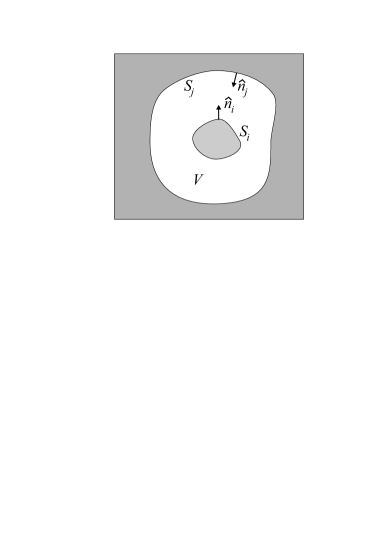
Figure 1: Configuration of two conductors in which the inner conductor with external surface $S_{i}$ is enclosed within the cavity of an external conductor. The surface of the cavity is denoted by $S_{j}$, and the volume$\ V$ is the region (in white) between both surfaces. We could interchange the role of the labels $i\leftrightarrow j$, and all our developments are still valid.

The BHF’s described in section 1 have an interesting application in determining coefficients of capacitance of certain geometrical configurations. Let us assume that the surfaces $S_{i}$ and $S_{j}$ defined in section 1 are covered by electrostatic conductors and the volumen $V$ is left empty. For example, let us assume for a moment that $S_{j}$ contains to $S_{i}$. We could have a conductor with a cavity such that the surface of the cavity is $S_{j}$ and we could have another conductor inside the cavity whose external surface is $S_{i}$ as displayed in Fig. 1. Of course, it is possible to interchange the roles of $S_{i}$ and $S_{j}$ and our developments are still the same.

We can determine the coefficients of capacitance for this geometry of capacitors by using the BHF’s in section 1. It can be shown that the coefficients of capacitance for the previous configuration of conductors are given by [3]

$$C_{ij}=-\varepsilon_{0}\oint_{S_{i}}\nabla f_{j}\left(u_{i}\right)\cdot\mathbf{n}_{i}dS$$ (42)

where $\mathbf{n}_{i}$ is a normal to the surface $S_{i}$ that points outwards with respect to the $i-th\$conductor. We have

$$Q_{i}=\sum_{j}C_{ij}\phi_{j}$$ (43)

with $Q_{i},\phi_{i}$ denoting the charge and potential on each conductor. Expression (42) is valid even if $i=j$. Nevertheless, we shall consider the case in which $i\neq j$ henceforth. Since the functions $f_{j}$ take constant values on each surface, then $\nabla f_{j}$ evaluated on each surface is perpendicular to such a surface. Moreover, it can be proved that [3]

$$\nabla f_{j}\left(u_{i},v,w\right)\cdot\mathbf{n}_{i}\geq 0\text{ \ for\ }i\neq j$$ (44)

such that $\nabla f_{j}\left(u_{i},v,w\right)$ is parallel (and not antiparallel) to $\mathbf{n}_{i}$ in each point $u_{i},v,w$ on the surface$\ S_{i}$. From these facts and using Eqs. (22, 23), as well as the fact that $f_{j}\left(u\right)$ only depends on $u$, we have

$$\nabla f_{j}\left(u_{i},v,w\right)\cdot\mathbf{n}_{i} = \left\|\nabla f_{j}\left(u_{i},v,w\right)\right\|=\left|\frac{1}{h_{u}\left(u_{i},v,w\right)}\frac{df_{j}\left(u_{i}\right)}{du}\right|=\left|\frac{1}{h_{u}\left(u_{i},v,w\right)~{}\left[Z\left(u_{j}\right)-Z\left(u_{i}\right)\right]}\frac{dZ\left(u_{i}\right)}{du}\right|$$

$$\nabla f_{j}\left(u_{i},v,w\right)\cdot\mathbf{n}_{i} = \left|\frac{1}{h_{u}\left(u_{i},v,w\right)~{}\left[Z\left(u_{j}\right)-Z\left(u_{i}\right)\right]G\left(u_{i}\right)}\right|$$ (45)

where we have taken into account that all functions involved in integral (42) should be evaluated at a given point in $S_{i}$ i.e. at $u=u_{i}$. Moreover, since $\mathbf{n}_{i}~{}dS$ is orthogonal to the unit vectors $\mathbf{e}_{v}$ and $\mathbf{e}_{w}$ associated with the $v,w$ coordinates, we have

$$dS=\left|h_{v}\left(u_{i},v,w\right)~{}h_{w}\left(u_{i},v,w\right)\right|dvdw$$

where we have taken into account that $dS$ is positive definite. Utilizing Eqs. (12) the differential of surface becomes

$$dS=\left|h_{u}\left(u_{i},v,w\right)~{}G\left(u_{i}\right)~{}H\left(v,w\right)\right|\ dv\ dw$$ (46)

substituting (45) and (46) in (42) the non-diagonal coefficients of capacitance yield finally

$$C_{ij}=-\frac{\varepsilon_{0}}{\left|Z\left(u_{j}\right)-Z\left(u_{i}\right)\right|}\oint_{S_{i}}\left|H\left(v,w\right)\right|dv~{}dw\ ;\ \ \text{with\ \ }i,j=1,2\ \ \text{and\ \ }i\neq j$$ (47)

we emphasize that despite Eq. (42) is valid for any values of $i$ and $j$, Eqs. (45) and (44) are only valid for $i\neq j$. In order to obtain the diagonal coefficients we only have to use the properties [3]

$$C_{i1}+C_{i2}=0\ ;\ \ C_{ij}=C_{ji}\ \ \Rightarrow\ \ C_{ii}=-C_{ij}\ \ \text{with\ \ }i,j=1,2\ \ \text{and\ \ }i\neq j$$

or more explicitly

$$C_{11}=C_{22}=-C_{12}=-C_{21}$$ (48)

It worths noting that expression (47) is also invariant under the “gauge transformations” given by Eqs. (25). On the other hand, Eqs. (47) and (48) leads to [3, 4]

$$C_{ii}>0\text{ and }C_{ij}<0\text{ \ with\ }i\neq j$$ (49)

Finally, as a proof of consistency, we see from Eq. (48) that the eigenvalues of the 2$\times 2$ matrix of capacitance are $0$ and$\ 2C_{11}$. These results along with Eqs. (49) says that the matrix of capacitance is positive singular as it must be [4]. In terms of voltages Eqs. (43, 48) becomes

$$Q_{1}=C_{11}\left(\phi_{1}-\phi_{2}\right)=C_{22}\left(\phi_{1}-\phi_{2}\right)=-Q_{2}$$ (50)

Note that if $S_{i}$ refers to the internal conductor, $Q_{i}$ is the total charge on it. But if $S_{i}$ refers to the cavity of the external conductor that contains the other conductor, $Q_{i}$ is only the charge accumulated on the surface of the cavity. In addition, if the internal conductor has a cavity, the surface of such a cavity does not contribute in the surface integral to calculate the coefficients of capacitance [2].

3.1 Capacitance for the particular case of the scale factors

As it was the case for the solutions of Laplace’s equation, the expression for the coefficients of capacitance is particularly simple when the system of coordinates obeys relation (26)

$$\frac{h_{v}h_{w}}{h_{u}}=1$$ (51)

in that case, Eqs. (27) provide simple solutions for $Z\left(u\right)$ and $H\left(v,w\right)$. Substituting (27) in Eq. (47), the latter becomes

$$C_{ij}=-\frac{\varepsilon_{0}}{\left|u_{j}-u_{i}\right|}\oint_{S_{i}}dv~{}dw\ \ ;\ \ i\neq j$$ (52)

or for the diagonal elements

$$C_{ii}=-C_{ij}=\frac{\varepsilon_{0}}{\left|u_{j}-u_{i}\right|}\oint_{S_{i}}dv~{}dw\ \ ;\ \ \text{with\ \ }i,j=1,2\ \ \text{and\ \ }i\neq j$$ (53)

We saw that Eq. (51) holds when we have a system of coordinates with cylindrical symmetry obtained with a conformal transformation from the cartesian coordinates. Nevertheless, we should recall that a cylindrical symmetry coming from a conformal transformation is only a sufficient condition. We only require the condition (51) to guarantee the validity of Eq. (53).

Observe that Eq. (53) has a structure similar to the capacitance of two parallel plates with “area”

$$A_{eff}\equiv\oint_{S_{i}}dv~{}dw$$ (54)

located at a “distance” $\left|u_{j}-u_{i}\right|$. Note however that in generalized coordinates, the integral (54) is not necessarily an area. For instance, if the two coordinates $v$ and $w$ are angular, this quantity is dimensionless. In the same way, the quantity $\left|u_{j}-u_{i}\right|$ is not always a distance.

3.2 Capacitance of two concentric spheres

Once again for the sake of illustration, we start calculating the well known capacitance of two concentric spheres with the values given in subsection 1.2. Thus, the radius of the smaller sphere is$\ b$ and the radius of the cavity of the bigger sphere is $a$, so that $a>b$. Applying Eqs. (31) and (32) in Eq. (47) and setting $r_{i}=r_{1}\equiv b$,$\ r_{j}=r_{2}\equiv a\$we get

$$C_{12} = -\frac{\varepsilon_{0}}{\left|Z\left(r_{2}\right)-Z\left(r_{1}\right)\right|}\oint_{S_{1}}\left|H\left(\theta,\varphi\right)\right|~{}d\theta~{}d\varphi=-\frac{\varepsilon_{0}}{\left|\frac{1}{a}-\frac{1}{b}\right|}\oint_{S_{1}}\left|\sin\theta\right|~{}d\theta~{}d\varphi$$

$$C_{12} = -\frac{\varepsilon_{0}ab}{\left(a-b\right)}\int_{0}^{\pi}\sin\theta~{}d\theta~{}\int_{0}^{2\pi}d\varphi=-\frac{4\pi\varepsilon_{0}ab}{\left(a-b\right)}$$

it is straigthforward that $C_{21}=C_{12}$. Therefore the coefficients of capacitance yield the expected result

$$C_{ii}=-C_{ij}=\frac{4\pi\varepsilon_{0}ab}{a-b}\ \ ;\ \ \text{with\ \ }i,j=1,2\ \ \text{and\ \ }i\neq j$$ (55)

3.3 Capacitance of two concentric cylinders

As for the case of BHF’s, it is more convenient to use the conformal polar cylindrical coordinates $\left(\rho,\varphi,z\right)$ defined by Eqs. (36) instead of the usual polar cylindrical system. Since for the $\left(\rho,\varphi,z\right)$ system the condition (51) is fullfilled the capacitance coefficients are given by Eq. (53)

$$C_{ii} = \frac{\varepsilon_{0}}{\left|\rho_{j}-\rho_{i}\right|}\oint_{S_{i}}d\varphi~{}dz=\frac{\varepsilon_{0}}{\left|\rho_{j}-\rho_{i}\right|}\int_{0}^{2\pi}d\varphi~{}\int_{-L/2}^{L/2}dz$$

$$C_{ii} = -C_{ij}=\frac{2\pi\varepsilon_{0}L}{\left|\rho_{j}-\rho_{i}\right|}=\frac{2\pi\varepsilon_{0}L}{\left|\ln\left(a/b\right)\right|}\ \ ;\ \ i,j=1,2\ \ \text{and\ \ }i\neq j$$ (56)

where we have assumed that the cylinders are located in the $z$ interval $\left[-L/2,\ L/2\right]$ with $L>>a$. This is the usual result.

4 Calculations of BHF’s and capacitances in more complex geometries

As we said, the cases of two concentric spheres and two concentric cylinders were developed for the sake of illustration only. In this section, we shall calculate BHF’s and capacitance coefficients for more complex symmetries in which our method acquires all its power.

4.1 BHF’s and capacitance on Prolate spheroidal surfaces

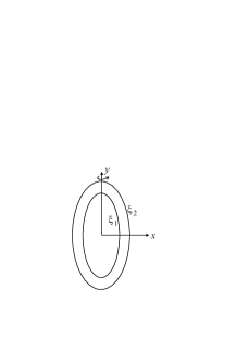
Figure 2: Shell formed between two confocal prolate spheroids.

Let us consider a shell formed between two confocal prolate spheroids as illustrated in Fig. 2. In order to find the BHF’s and capacitance coefficients, we use the Prolate spheroidal system of coordinates, which is obtained by revolutioning the elliptical bidimensional system of coordinates $\left(\xi,\eta\right)\$with respect to the major semiaxis of the ellipses. The most usual definition of the prolate spheroidal system of coordinates reads:

$$x = a\sinh\xi\sin\eta\cos\varphi\ \ ;\ \ y=a\sinh\xi\sin\eta\sin\varphi\ \ ;\ \ z=a\cosh\xi\cos\eta$$

$$\xi \geq 0,\ \ \eta\in[0,\pi],\ \ \ a=\frac{d}{2}\ \ ;\ \ \varphi\in[0,2\pi)$$

where $\xi,\eta$ are the bidimensional elliptical coordinates, $\varphi$ is the azimuthal angle and $d$ denotes the distance between the foci. The scale factors are given by

$$h_{\xi}=h_{\eta}=a\sqrt{\sinh^{2}\xi+\sin^{2}\eta}\ \ ;\ \ h_{\varphi}=a\sinh\xi\sin\eta$$ (57)

By means of the trigonometric and hyperbolic identities

$$\frac{z^{2}}{a^{2}\cosh^{2}\xi}+\frac{x^{2}+y^{2}}{a^{2}\sinh^{2}\xi} = \cos^{2}\eta+\sin^{2}\eta=1$$ (58)

$$\frac{z^{2}}{a^{2}\cos^{2}\eta}-\frac{x^{2}+y^{2}}{a^{2}\sin^{2}\eta} = \cosh^{2}\xi-\sinh^{2}\xi=1$$ (59)

it can be seen that the constant values of $\xi$ correspond to prolate spheroids, while surfaces of constant $\eta$ are hyperboloids of revolution. Consequently, since we are interested in the configuration in which the surfaces are confocal prolate spheroids, the coordinate that is kept constant is $\xi$. Then we shall assign $\left(u,v,w\right)\rightarrow\left(\xi,\eta,\varphi\right)$. Combining Eqs. (57) and (23) we have

$$\frac{h_{\eta}h_{\varphi}}{h_{\xi}}=h_{\varphi}=a\sinh\xi\sin\eta\equiv G\left(\xi\right)H\left(\eta,\varphi\right)$$

Such that a set of solutions for $G\left(u\right)$ and $H\left(v,w\right)$ is given by

$$G\left(\xi\right)=a\sinh\xi\ \ ;\ \ H\left(\eta,\varphi\right)=\sin\eta$$ (60)

and from Eqs. (23, 60), the simplest solution for $Z\left(u\right)$ yields

$$Z\left(\xi\right) = \int\frac{d\xi}{G\left(\xi\right)}=\frac{1}{a}\int\frac{1}{\sinh\xi}\ d\xi$$

$$Z\left(\xi\right) = \frac{1}{a}\ln\left(\tanh\frac{\xi}{2}\right)$$ (61)

substituting (61) in (22) we obtain

$$f_{j}\left(\xi\right) = \frac{Z\left(\xi\right)-Z\left(\xi_{i}\right)}{\left[Z\left(\xi_{j}\right)-Z\left(\xi_{i}\right)\right]}$$

$$f_{j}\left(\xi\right) = \frac{\ln\left(\tanh\frac{\xi}{2}\right)-\ln\left(\tanh\frac{\xi_{i}}{2}\right)}{\ln\left(\tanh\frac{\xi_{j}}{2}\right)-\ln\left(\tanh\frac{\xi_{i}}{2}\right)}=\frac{\ln\left(\frac{\tanh\frac{\xi}{2}}{\tanh\frac{\xi_{i}}{2}}\right)}{\ln\left(\frac{\tanh\frac{\xi_{j}}{2}}{\tanh\frac{\xi_{i}}{2}}\right)}\ \ ;\ \ i,j=1,2\text{\ \ and\ \ }i\neq j$$ (62)

where $\xi_{i}$ and $\xi_{j}$ are the constant values of that coordinate on the surfaces $S_{i}$ and $S_{j}$. Now for the capacitance we subtitute (60) and (61) in (47) to get

$$C_{12} = -\frac{\varepsilon_{0}}{\left|Z\left(\xi_{2}\right)-Z\left(\xi_{1}\right)\right|}\oint_{S_{1}}\left|H\left(\eta,\varphi\right)\right|~{}d\eta~{}d\varphi$$

$$C_{12} = -\frac{\varepsilon_{0}}{\left|\frac{1}{a}\ln\left(\tanh\frac{\xi_{2}}{2}\right)-\frac{1}{a}\ln\left(\tanh\frac{\xi_{1}}{2}\right)\right|}\int_{0}^{2\pi}~{}d\varphi\int_{0}^{\pi}\sin\eta~{}d\eta$$

the explicit calculation of $C_{21}$ gives $C_{21}=C_{12}$ as it must be. So we finally obtain

$$C_{ii}=-C_{ij}=\frac{4\pi a\varepsilon_{0}}{\left|\ln\left(\frac{\tanh\frac{\xi_{j}}{2}}{\tanh\frac{\xi_{i}}{2}}\right)\right|}\ \ ;\ \ i,j=1,2\text{\ \ and\ \ }i\neq j$$ (63)

The reader can contrast the simplicity and brevity of the calculation in this subsection, with respect to the methods developed in the literature (see for instance Ref. [25]). Once the general formulas (22, 23) and (47) are obtained, the application to this specific geometry is just a bit more than a direct replacement. This is also the case with other symmetries as we shall see.

Finally, it is desirable to obtain the capacitance in terms of geometrical factors. Defining $a_{i}$ as the major semiaxes of the prolate spheroid associated with $\xi_{i}$, the capacitance (63) becomes (see appendix C)

$$C_{ii}=-C_{ij}=\frac{4\pi a\varepsilon_{0}}{\left|\ln\left(\frac{\left(a+a_{i}\right)\sqrt{a_{j}^{2}-a^{2}}}{\left(a+a_{j}\right)\sqrt{a_{i}^{2}-a^{2}}}\right)\right|}\ \ ;\ \ i,j=1,2\text{\ \ and\ \ }i\neq j$$ (64)

it is also shown in appendix C that the capacitance of two concentric spheres is obtained from the limit where $a$ tends to zero.

4.2 BHF’s and capacitance on oblate spheroidal surfaces

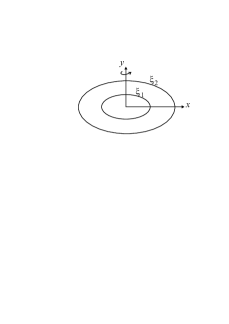
Figure 3: A shell formed between two confocal oblate spheroidal surfaces.

Let us consider a shell formed between two confocal oblate spheroids as displayed in Fig. 3. Then, we should work with the oblate spheroidal coordinate system which is obtained by revolutioning the bidimensional elliptical coordinate system $\left(\xi,\eta\right)\$around the minor semiaxis of the ellipses. The transformation of coordinates and scale factors yield

$$x = a\cosh\xi\cos\eta\cos\varphi\ \ ;\ \ y=a\cosh\xi\cos\eta\sin\varphi\ \ ;\ \ z=a\sinh\xi\sin\eta$$ (65)

$$h_{\xi} = h_{\eta}=a\sqrt{\sinh^{2}\xi+\sin^{2}\eta}\ \ ;\ \ h_{\varphi}=a\cosh\xi\cos\eta$$ (66)

$$\xi \geq 0,\ \ \eta\in[-\frac{\pi}{2},\frac{\pi}{2}],\ \ \ a=\frac{d}{2}\ \ ;\ \ \varphi\in[0,2\pi)$$ (67)

The trigonometric and hyperbolic identities

$$\frac{z^{2}}{a^{2}\sinh^{2}\xi}+\frac{x^{2}+y^{2}}{a^{2}\cosh^{2}\xi} = \cos^{2}\eta+\sin^{2}\eta=1$$ (68)

$$\frac{x^{2}+y^{2}}{a^{2}\cos^{2}\eta}-\frac{z^{2}}{a^{2}\sin^{2}\eta} = \cosh^{2}\xi-\sinh^{2}\xi=1$$ (69)

show that the surfaces in which $\xi\$acquires constant values correspond to oblate spheroids, while the surfaces with $\eta$ constant correspond to hyperboloids of revolution. Once again, $\xi$ is the variable that is kept constant in the surfaces we are working with. Equations (23) and (66) are combined to give

$$\frac{h_{\eta}h_{\varphi}}{h_{\xi}} = h_{\varphi}=a\cosh\xi\cos\eta\equiv G\left(\xi\right)H\left(\eta,\varphi\right)$$

$$G\left(\xi\right) \equiv a\cosh\xi\ \ ;\ \ H\left(\eta,\varphi\right)\equiv\cos\eta$$ (70)

$$Z\left(\xi\right) = \frac{1}{a}\int\frac{1}{\cosh\xi}d\xi=\frac{1}{a}\sin^{-1}\left(\tanh\xi\right)$$ (71)

Using Eqs. (70, 71) in (22) we obtain

$$f_{j}\left(\xi\right)=\frac{Z\left(\xi\right)-Z\left(\xi_{i}\right)}{\left[Z\left(\xi_{j}\right)-Z\left(\xi_{i}\right)\right]}=\frac{\sin^{-1}\left(\tanh\xi\right)-\sin^{-1}\left(\tanh\xi_{i}\right)}{\sin^{-1}\left(\tanh\xi_{j}\right)-\sin^{-1}\left(\tanh\xi_{i}\right)}\ \ ;\ \ i,j=1,2\text{\ \ and\ \ }i\neq j$$ (72)

and the capacitance coefficients are obtained from (70, 71) and (47)

$$C_{ij} = \frac{-\varepsilon_{0}}{\left|Z\left(\xi_{j}\right)-Z\left(\xi_{i}\right)\right|}\oint_{S_{1}}\left|H\left(\eta,\varphi\right)\right|~{}d\eta~{}d\varphi=\frac{-\varepsilon_{0}}{\left|\frac{1}{a}\sin^{-1}\left(\tanh\xi_{j}\right)-\frac{1}{a}\sin^{-1}\left(\tanh\xi_{i}\right)\right|}\int_{0}^{2\pi}d\varphi\int_{-\pi/2}^{\pi/2}\cos\eta~{}d\eta$$

$$C_{ii} = -C_{ij}=\frac{4\pi a\varepsilon_{0}}{\left|\sin^{-1}\left(\tanh\xi_{j}\right)-\sin^{-1}\left(\tanh\xi_{i}\right)\right|}\ \ ;\ \ i,j=1,2\text{\ \ and\ \ }i\neq j$$ (73)

for instance, if we compare with the procedure in Ref. [26], the advantages of our method are apparent. In terms of geometrical factors the coefficients $C_{ij}$ read (see appendix C)

$$C_{ii}=-C_{ij}=\frac{4\pi a\varepsilon_{0}}{\left|\cos^{-1}\epsilon_{j}-\cos^{-1}\epsilon_{i}\right|}\ \ ;\ \ i,j=1,2\text{\ \ and\ \ }i\neq j$$ (74)

where $\epsilon_{j}$,$\ \epsilon_{i}$ are the eccentricities of the ellipses associated with the surfaces $S_{j}$ and $S_{i}$ respectively.

4.3 BHF’s and capacitance of two confocal elliptical cylinders

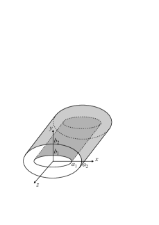
Figure 4: A shell formed between two confocal elliptical cylinders. The values $a_{1},~{}a_{2}$ correspond to the major semiaxes, while $b_{1},~{}b_{2}$ denote the minor semiaxes.

This is an example in which the particular condition (26) is fulfilled. Let us consider a shell formed by two confocal elliptical cylinders as shown in Fig. 4. The values $b_{1}$, $a_{1}$, correspond to the minor semiaxis and major semiaxis of the internal cylinder, while $b_{2}$, $a_{2}$ are the semiaxes associated with the external cylinder. We assume that along the $Z-$axis the cylinders are located in the interval $\left[-L/2,~{}L/2\right]$ with $L>>a_{2}$. We shall use the cylindrical elliptical system of coordinates which is obtained by projecting the elliptical bidimensional system on the $Z-$axis. The transformation of coordinates and scale factors yield

$$x = a\cosh\xi\cos\eta\ ;\ y=a\sinh\xi\sin\eta\ \ ;\ z=z$$ (75)

$$h_{\xi} = h_{\eta}=a\sqrt{\sinh^{2}\xi+\sin^{2}\eta}\ \ ;\ \ h_{z}=1$$ (76)

$$\xi \geq 0\ ;\ \ 0\leq\eta<2\pi\ ;\ \ -\infty<z<\infty\ ;\ \ a=\frac{d}{2}$$ (77)

The trigonometrical and hyperbolic identities

$$\frac{x^{2}}{a^{2}\cosh^{2}\xi}+\frac{y^{2}}{a^{2}\sinh^{2}\xi} = \cos^{2}\eta+\sin^{2}\eta=1$$ (78)

$$\frac{x^{2}}{a^{2}\cos^{2}\eta}-\frac{y^{2}}{a^{2}\sin^{2}\eta} = \cosh^{2}\xi-\sinh^{2}\xi=1$$ (79)

say that surfaces with constant $\xi$ are confocal elliptical cylinders and surfaces with $\eta$ constant are confocal hyperbolic cylinders. Thus $\xi$ is the coordinate that takes constant values in the surfaces we are considering. Equation (76) shows that in this case, the condition (26) is satisfied. Consequently, the BHF’s are given by Eq. (28) that in this case becomes

$$f_{j}\left(\xi\right)=\frac{\xi-\xi_{i}}{\xi_{j}-\xi_{i}}\ \ ;\ \ i,j=1,2\text{\ \ and\ \ }i\neq j$$ (80)

and the coefficients of capacitance are given by Eq. (53) that in our case gives

$$C_{11} = -C_{12}=\frac{\varepsilon_{0}}{\left|\xi_{2}-\xi_{1}\right|}\oint_{S_{1}}d\eta\ dz=\frac{\varepsilon_{0}}{\left|\xi_{2}-\xi_{1}\right|}\int_{0}^{2\pi}d\eta\int_{-L/2}^{L/2}dz$$

$$C_{ii} = -C_{ij}=\frac{2\pi\varepsilon_{0}L}{\left|\xi_{i}-\xi_{j}\right|}\ \ ;\ \ i,j=1,2\text{\ \ and\ \ }i\neq j$$ (81)

Note that the integral has the same value if we integrate over $S_{2}$, it guarantees that $C_{12}=C_{21}$. This example shows that under the condition (26) the results are much simpler. In terms of geometrical factors Eq. (81) becomes (see appendix C)

$$C_{ii}=-C_{ij}=\frac{2\pi\varepsilon_{0}L}{\left|\ln\left[\frac{a_{i}+\sqrt{a_{i}^{2}-a^{2}}}{a_{j}+\sqrt{a_{j}^{2}-a^{2}}}\right]\right|}\ \ ;\ \ i,j=1,2\text{\ \ and\ \ }i\neq j$$ (82)

the limit $a\rightarrow 0$, reduces to the case of two concentric cylinders.

4.4 BHF’s and capacitance of two eccentric cylinders

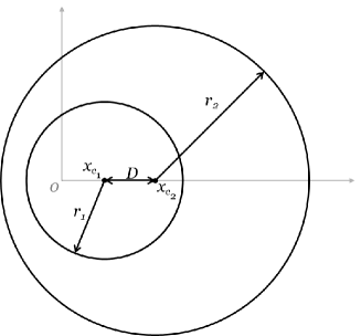
Figure 5: Two eccentric cylinders $C_{1}$ and $C_{2}\$with radii $r_{1}$ and $r_{2}$. The cylinder $C_{1}$ is contained in the cylinder $C_{2}$, and their centers are separated by a distance $D$.

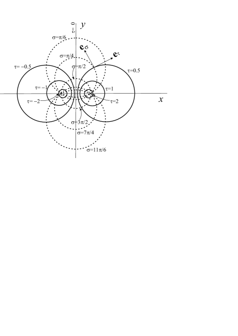
Figure 6: Bipolar coordinate system (in two dimensions) with foci $F_{1}=\left(0,-a\right)$ and $F_{2}=\left(0,a\right)$. It is shown that curves associated with positive (negative) constant values of $\tau$ are circles that contain the focus $F_{2}\$($F_{1}$). When $\left|\tau_{1}\right|>\left|\tau_{2}\right|$ the circle $C_{2}$ contains the circle $C_{1}$.

Let us consider a shell like the one in Fig. 5. The external cylinder has a radius $r_{2}$, and the internal one a radius $r_{1}$. The centers are located at the points $\left(x_{c_{1}},0\right)$ and $\left(x_{c_{2}},0\right)$, and are separated by a distance $D$. The cylindrical bipolar coordinate system is the appropriate for this geometry. The (bidimensional) bipolar coordinate system posseses two foci $F_{1}$ and $F_{2}$, usually located at $(-a,0)$ and $(a,0)$ respectively. The transformations from cartesian coordinates and scale factors are given by

$$x = a\frac{\sinh\tau}{\cosh\tau-\cos\sigma}\ \ ;\ \ y=a\frac{\sin\sigma}{\cosh\tau-\cos\sigma}\ \ ;\ \ z=z$$

$$h_{\sigma} = h_{\tau}=\frac{a}{\cosh\tau-\cos\sigma}\ ;\ h_{z}=1$$

$$0 \leq \sigma<2\pi\ \ ;\ \ -\infty<\tau<+\infty\ \ ;\ \ -\infty<z<+\infty$$

The distance from each focus to an arbitrary point $\left(x,y\right)\$in the plane yields

$$d_{1}^{2}=(x+a)^{2}+y^{2}\ \ ;\ d_{2}^{2}=(x-a)^{2}+y^{2}$$

Thus, $\sigma$ represents the angle between the lines that join each focus with a given point $\left(x,y\right)$ in the plane, while $\tau$ is given by

$$\tau=\ln\left(\frac{d_{1}}{d_{2}}\right)$$

the curves (in the plane) with $\sigma$ constant correspond to non-concentric circles that intersect in the two foci (see Fig. 6). The curves with $\tau$ constant correspond to non-intersecting circles and with different radii (see Fig. 6). Two curves $C_{1}$ and $C_{2}\$with constant positive values $\tau_{1}>\tau_{2}$ correspond to two non-concentric circles such that both circles contain the focus $F_{2}$ and the circle $C_{2}$ contains the circle $C_{1}$. Adding the $z$ coordinate, we obtain the desire configuration of two non-concentric cylinders. Therefore, we assign $\left(u,v,w\right)\rightarrow\left(\tau,\sigma,z\right)$. Note that this system of coordinates satisfy condition (26) so that the solutions for the coefficients of capacitance and BHF’s are given by Eqs. (28) and (53)

$$f_{j}\left(\tau\right) = \frac{\tau-\tau_{i}}{\tau_{j}-\tau_{i}}\ \ ;\ \ i,j=1,2\text{ and }i\neq j$$ (83)

$$C_{ii} = \frac{\varepsilon_{0}}{\left|\tau_{j}-\tau_{i}\right|}\oint_{S_{i}}d\sigma~{}dz=\frac{\varepsilon_{0}}{\left|\tau_{j}-\tau_{i}\right|}\int_{0}^{2\pi}d\sigma~{}\int_{-L/2}^{L/2}dz$$

$$C_{ii} = -C_{ij}=\frac{2\pi\varepsilon_{0}L}{\left|\tau_{j}-\tau_{i}\right|}\ \ ;\ \ i,j=1,2\text{ and }i\neq j$$ (84)

Substituting Eq. (122) of appendix C in Eq. (84), we obtain the coefficients of capacitance in terms of geometrical factors

$$C_{ii}=-C_{ij}=\frac{2\pi\varepsilon_{0}L}{\cosh^{-1}\left(\frac{r_{1}^{2}+r_{2}^{2}-D^{2}}{2r_{1}r_{2}}\right)}$$ (85)

when $D\rightarrow 0$ we recover the expression for two concentric cylinders.

5 Conclusions

We solve Laplace’s equation for some geometrical configurations in which there exist a system of coordinates $\left(u,v,w\right)\$that can be adjusted to the geometry. Specifically, we assume that the boundary consists of two closed surfaces $S_{1}$ and $S_{2}$ so that one of the surfaces is included into the other, and in which the coordinate $u\$takes constant values $u_{1}$ and $u_{2}$ on each surface $S_{1}$ and $S_{2}$. We solve Laplace’s equation within the volume $V$ between both surfaces. Besides, we take specific boundary conditions in which the solutions take values that are either zero or unity on the surfaces. The solutions of Laplace’s equation with such specific boundary conditions are called Basic Harmonic Functions (BHF’s). It worths remarking that the BHF’s only depend on the geometry, and their solutions via separation of variables are particularly simple. The expressions for the BHF’s are given in terms of generalized curvilinear coordinates in such a way that we can sweep a variety of systems of coordinates to obtain the BHF’s associated with the given symmetry.

Further, we exploit the purely geometrical BHF’s in two ways. On one hand, we can determine a more general class of Harmonic Functions (HF’s i.e. solutions of Laplace’s equation) for the same geometry of the BHF’s, but in which the functions take arbitrary constant values on the boundaries. On the other hand, we calculate the coefficients of capacitance when the surfaces that form the volume are covered with electrostatic conductors. Expressions for either HF’s and for coefficients of capacitance are given again in terms of generalized curvilinear coordinates, such that we can obtain these quantities for multiple symmetries by simple replacements. Several examples with different symmetries are provided.

In addition, appendices A and B show natural extensions coming from our present formulation. In appendix A, expressions for the electric field between two conductors and the charge densities on each of their surfaces are written in generalized curvilinear coordinates, while in appendix B, formulas for the capacitance coefficients are extended to the case of conductors in sucessive embedding.

It worths emphasizing that after obtaining the general formulas for BHF’s, capacitance coefficients, electric fields and surface charge densities in terms of generalized orthogonal curvilinear coordinates, calculations of these observables for each symmetry are straightforward. After checking Eqs. (22, 23, 47) and Eqs. (88, 89) we can see that all those observables are obtained by simple combinations of the functions $h_{u},G\left(u\right),\ H\left(v,w\right)$ and $Z\left(u\right)$. The first three are basically input parameters, and the latter is obtained from $1/G\left(u\right)$ by a direct integration. Comparison with the calculations of the same quantities with other methods given in the literature, shows the simplicity and brevity of our method as it was emphasized in several of our examples.

Note that despite with the traditional strategies Laplace’s Equation can be solved in many cases via separation of variables, in most of such cases a series expansion in certain special functions is usually required in order to adjust the boundary conditions. By contrast, the BHF’s obtained via the formulas (22, 23) lead in many problems to closed solutions. Therefore, solutions of Laplace’s equation with equipotential surfaces can often be written (with our method) in terms of closed well-defined functions. Though solutions in series are exact in principle, when we handle them in practice we should truncate the series somewhere, leading to a considerable expansion of numerical errors, especially if the series converges slowly (sometimes problems of convergence also arise).

On the other hand, it is well known that solutions of Laplace’s equation can be treated with the geometrical formalism of Green’s functions. Nevertheless, it could be noticed that finding BHF’s (which are also purely geometrical) is in general much easier than the calculation of the Green’s function on the same geometry. Finally, it is possible to extrapolate the method developed here to other linear homogeneous differential equations. In the same way that we can associate a Green’s function with each linear differential operator, we can define BHF’s for each linear differential operator.

Appendix A Electric field and surface density in a configuration of two conductors

Once again we use $i,j=1,2$ and $i\neq j$ throughout this section. If $\phi_{i}$ and $\phi_{j}$ are the (constant) potentials on conductors $i$ and $j$ respectively, the potential in the volume $V$ between the surfaces $S_{i}$ and $S_{j}$ is given by Eq. (39)

$$\phi=\phi_{i}f_{i}+\phi_{j}f_{j}$$ (86)

on the other hand, from the property $f_{i}+f_{j}=1$ we obtain

$$\nabla f_{i}=-\nabla f_{j}$$ (87)

combining Eqs. (86, 87) and the fact that the BHF’s only depend on $u$, we can find the electric field within the volume $V\$in terms of curvilinear coordinates

$$\mathbf{E}=-\nabla\phi=-\phi_{i}\nabla f_{i}-\phi_{j}\nabla f_{j}=\left(\phi_{i}-\phi_{j}\right)\nabla f_{j}=\frac{\phi_{i}-\phi_{j}}{h_{u}\left(u,v,w\right)}\frac{\partial f_{j}\left(u\right)}{\partial u}\mathbf{e}_{u}\left(u,v,w\right)$$

where $\mathbf{e}_{u}\left(u,v,w\right)$ is the local unitary vector associated with the $u\$coordinate. Using Eqs. (22, 23) we have

$$\mathbf{E}\left(u,v,w\right) = \frac{\phi_{i}-\phi_{j}}{h_{u}\left(u,v,w\right)~{}\left[Z\left(u_{j}\right)-Z\left(u_{i}\right)\right]}\frac{dZ\left(u\right)}{du}\mathbf{e}_{u}\left(u,v,w\right)$$

$$\mathbf{E}\left(u,v,w\right) = \frac{\phi_{i}-\phi_{j}}{h_{u}\left(u,v,w\right)~{}\left[Z\left(u_{j}\right)-Z\left(u_{i}\right)\right]~{}G\left(u\right)}\mathbf{e}_{u}\left(u,v,w\right)\ \ ;\ \ i,j=1,2\ \ \text{and }i\neq j$$ (88)

On the other hand, the surface charge density induced on the surface $S_{i}$ of a perfect conductor is given by [2]

$$\sigma\left(S_{i}\right)=\sigma\left(u_{i},v,w\right)=-\varepsilon_{0}\nabla\phi\left(u_{i},v,w\right)\cdot\mathbf{n}_{i}=\varepsilon_{0}\left(\phi_{i}-\phi_{j}\right)\nabla f_{j}\left(u_{i},v,w\right)\cdot\mathbf{n}_{i}$$

where we have used Eqs. (86) and (87). Finally, by using Eq. (45) we have

$$\sigma\left(u_{i},v,w\right)=\left|\frac{\varepsilon_{0}}{h_{u}\left(u_{i},v,w\right)~{}\left[Z\left(u_{j}\right)-Z\left(u_{i}\right)\right]G\left(u_{i}\right)}\right|\left(\phi_{i}-\phi_{j}\right)\ \ ;\ \ i,j=1,2\text{\ and\ }i\neq j$$ (89)

As a proof of consistency, let us obtain the total charge on the surface $S_{i}$. By using Eqs. (89, 46) and (47, 48) we obtain

$$Q_{i} = \oint_{S_{i}}\sigma\left(u_{i},v,w\right)~{}dS=\varepsilon_{0}\left(\phi_{i}-\phi_{j}\right)\oint_{S_{i}}\left|\frac{dS}{h_{u}\left(u_{i},v,w\right)~{}\left[Z\left(u_{j}\right)-Z\left(u_{i}\right)\right]G\left(u_{i}\right)}\right|$$

$$= \varepsilon_{0}\left(\phi_{i}-\phi_{j}\right)\oint_{S_{i}}\left|\frac{h_{u}\left(u_{i},v,w\right)~{}G\left(u_{i}\right)~{}H\left(v,w\right)}{h_{u}\left(u_{i},v,w\right)~{}\left[Z\left(u_{j}\right)-Z\left(u_{i}\right)\right]G\left(u_{i}\right)}\right|\ dv\ dw$$

$$= \left(\phi_{i}-\phi_{j}\right)\frac{\varepsilon_{0}}{\left|Z\left(u_{j}\right)-Z\left(u_{i}\right)\right|}\oint_{S_{i}}\left|H\left(v,w\right)\right|\ dv\ dw=-C_{ij}\left(\phi_{i}-\phi_{j}\right)$$

$$Q_{i} = C_{ii}\left(\phi_{i}-\phi_{j}\right)$$ (90)

which reproduces the correct expression (50) for the total charge on $S_{i}$. If we compare expressions (89) and (90), the term in the absolute value of Eq. (89) behaves like an “effective capacitance per unit area”. Effectively, such a term is purely geometrical, as is the term $C_{ii}$.

A.1 Electric fields and charge densities for two concentric spheres

For the two concentric spheres of Sec. 1.2, we substitute Eqs. (29, 31, 32) in Eq. (88) to obtain

$$\mathbf{E}\left(\mathbf{r}\right) = \frac{\left(\phi_{i}-\phi_{j}\right)\mathbf{e}_{r}}{h_{r}~{}\left[Z\left(r_{j}\right)-Z\left(r_{i}\right)\right]~{}G\left(r\right)}=\frac{\left(\phi_{1}-\phi_{2}\right)\mathbf{e}_{r}}{\left[\frac{1}{r_{2}}-\frac{1}{r_{1}}\right]~{}\left(-r^{2}\right)}=\frac{\left(\phi_{b}-\phi_{a}\right)\mathbf{e}_{r}}{\left[\frac{1}{a}-\frac{1}{b}\right]~{}\left(-r^{2}\right)}$$

$$\mathbf{E}\left(\mathbf{r}\right) = \frac{ab\left(\phi_{b}-\phi_{a}\right)}{\left(a-b\right)~{}r^{2}}\mathbf{e}_{r}$$ (91)

and substituting (29, 31, 32) in Eq. (89) we find

$$\sigma\left(r_{i}\right) = \left|\frac{\varepsilon_{0}}{h_{r}\left(r_{i}\right)~{}\left[\frac{1}{r_{j}}-\frac{1}{r_{i}}\right]\left(-r_{i}^{2}\right)}\right|\left(\phi_{i}-\phi_{j}\right)=\frac{r_{j}}{r_{i}}\frac{\varepsilon_{0}\left(\phi_{i}-\phi_{j}\right)}{\left|r_{i}-r_{j}\right|}$$

$$\sigma\left(a\right) = \frac{b}{a}\frac{\varepsilon_{0}\left(\phi_{a}-\phi_{b}\right)}{\left(a-b\right)}\ ;\ \ \sigma\left(b\right)=\frac{a}{b}\frac{\varepsilon_{0}\left(\phi_{b}-\phi_{a}\right)}{\left(a-b\right)}$$ (92)

integrating these densities on $S_{a}$ and $S_{b}$ we obtain the total charge on such surfaces. Further, taking into account Eqs. (55, 91) we obtain the consistency of all these results

$$Q_{a}=-Q_{b}=\frac{4\pi\varepsilon_{0}ab\left(\phi_{a}-\phi_{b}\right)}{\left(a-b\right)}=C_{11}\left(\phi_{a}-\phi_{b}\right)\ ;\ \ \mathbf{E}\left(\mathbf{r}\right)=\frac{Q_{b}}{4\pi\varepsilon_{0}r^{2}}\mathbf{e}_{r}$$

A.2 Electric fields and charge densities for a prolate spheroidal shell

For a prolate spheroidal shell, we obtain the electric field within the shell and the charge density on the ellipsoidal surfaces by substituting Eqs. (57, 60) and (61) in Eqs. (91, 92)

$$\mathbf{E}\left(\xi,\eta,\varphi\right) = \frac{\phi_{i}-\phi_{j}}{a\sqrt{\sinh^{2}\xi+\sin^{2}\eta}~{}\left[\ln\left(\tanh\frac{\xi_{j}}{2}\right)-\ln\left(\tanh\frac{\xi_{i}}{2}\right)\right]~{}\sinh\xi}\mathbf{e}_{\xi}\left(\xi,\eta,\varphi\right)$$

$$\sigma\left(u_{i},\eta,\varphi\right) = \left|\frac{\varepsilon_{0}}{a\sqrt{\sinh^{2}\xi_{i}+\sin^{2}\eta}~{}\left[\ln\left(\tanh\frac{\xi_{j}}{2}\right)-\ln\left(\tanh\frac{\xi_{i}}{2}\right)\right]~{}\sinh\xi_{i}}\right|\left(\phi_{i}-\phi_{j}\right)\ \ ;\ \ i,j=1,2\ \ \text{and\ \ }i\neq j$$

the magnitude of the electric field and the surface charge densities are independent of the azimutahl angle $\varphi$ as the symmetry suggests. Calculation of electric fields and surface charge densities in other complex geometries is also straightforward.

Appendix B Chains of embedded conductors

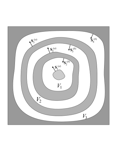
Figure 7: Configuration of succesive embedding of 4 conductors. The surface $S_{1}^{\left(a\right)}$ has only outer part while the surface $S_{4}^{\left(b\right)}$ has only an inner part (the surface of the cavity). Conductors 2 and 3 have an inner part $S_{i}^{\left(b\right)}\$and an outer part $S_{i}^{\left(a\right)}$.

Let us assume that we have a set of $N+1\$conductors succesively embedded as indicated in Fig. 7. We label them as$\ 1,2,\ldots,N+1$ from the inner to the outer. We can see that for $k=2,\ldots,N$ the surface $S_{k}$ of the $k-th$ conductor has an inner part that we denote as $S_{k}^{\left(b\right)}$, and an outer part that we denote as $S_{k}^{\left(a\right)}$. However, for $S_{1}$ we only have outer part, while for $S_{N+1}$ we only have an inner part. Nevertheless, we still preserve the inner and outer notation for $S_{1}$ and $S_{N+1}\$by writing $S_{1}=S_{1}^{\left(a\right)}$ and $S_{N+1}=S_{N+1}^{\left(b\right)}$. The volume $V_{k}$ with $k=1,\ldots,N$ is defined between $S_{k}^{\left(a\right)}$ and $S_{k+1}^{\left(b\right)}$.

A set of conductors in succesive embedding has some particular properties (see appendix C in Ref [4]). First, the only non-zero coefficients of capacitance are the diagonal ones $C_{ii}\$and the terms of the form $C_{i,i\pm 1}$. Of course, for $i=1$ there is no term of the form $C_{i,i-1}$, and for $i=N+1$ there is no term of the form $C_{i,i+1}$. The diagonal terms are related with the non-diagonal ones as follows

$$C_{ii} = -\left(C_{i,i-1}+C_{i,i+1}\right)\ \ \ ;\ \ \ i=2,\ldots,N$$

$$C_{11} = -C_{12}\ \ ;\ \ C_{N+1,N+1}=-C_{N,N+1}$$ (93)

now, owing to the symmetry of the matrix and the properties (93), it is enough to calculate the non-diagonal terms of the form $C_{i,i+1}$ for $i=1,\ldots,N$. It can also be proved that [4]

$$C_{i,i+1}=-\varepsilon_{0}\oint_{S_{i}^{\left(a\right)}}\nabla f_{i+1}\left(u_{i}^{\left(a\right)}\right)\cdot\mathbf{n}_{i}^{\left(a\right)}dS\ \ ;\ \ i=1,\ldots,N$$ (94)

that is, only the outer part of the surface $S_{i}$ contributes to the surface integral in the calculation of$\ C_{i,i+1}$. It worths pointing out that the properties described above are valid for any geometry of the conductors, the only condition is that they should be in succesive embedding.

Now let us add the hypotheses we have been working with. That is, that we have a curvilinear coordinate system $\left(u,v,w\right)$ such that the coordinate $u$ acquires a constant value $u_{p}^{\left(\mathcal{\lambda}\right)}$ on each surface $S_{p}^{\left(\lambda\right)}$ with $p=1,2,\ldots,N+1$ and $\lambda=a,b$.

First of all, we want to calculate the BHF’s within each volume $V_{i}$. By definition of the BHF’s, they satisfy the boundary conditions

$$f_{i}\left(S_{i}^{\left(\lambda\right)}\right)=1,\ \ f_{i}\left(S_{j}^{\left(\lambda\right)}\right)=0\ \ ;\ \ i\neq j\text{ \ and\ \ }\lambda=a,b$$ (95)

It could be shown that within the volumen $V_{i}$ the BHF’s have the following properties

$$f_{i}\left(V_{i}\right)+f_{i+1}\left(V_{i}\right)=1\ \ ;\ \ f_{i+k+1}\left(V_{i}\right)=f_{i-k}\left(V_{i}\right)=0\text{\ };\ \ i=1,2,\ldots,N\ \ ,\ \ k\geq 1$$

therefore, it is sufficient to calculate $f_{i+1}$ within the volume $V_{i}$. Our boundary conditions for the BHF $f_{i+1}$ within $V_{i}$ are given by

$$f_{i+1}\left(S_{i}^{\left(a\right)}\right)=0\ \ \ ;\ \ f_{i+1}\left(S_{i+1}^{\left(b\right)}\right)=1$$

with the same analysis done in section 1, we see that the functions $f_{i+1}$ only depends on $u$, such that these boundary conditions can be written as

$$f_{i+1}\left(u_{i}^{\left(a\right)}\right)=0\ \ \ ;\ \ f_{i+1}\left(u_{i+1}^{\left(b\right)}\right)=1$$ (96)

now, taking into account that in this context the volume $V_{i}$ in which we are evaluating the BHF’s is delimited by the two surfaces $S_{i}^{\left(a\right)}$ and $S_{i+1}^{\left(b\right)}$, we can use the same arguments that led to Eqs. (22) with the assignments

$$i\rightarrow i\ \ ,\ j\rightarrow i+1,\ u_{i}\rightarrow u_{i}^{\left(a\right)}\ ,\ \ u_{j}\rightarrow u_{i+1}^{\left(b\right)}$$ (97)

From these facts the function $f_{i+1}$ evaluated at any point within the volume $V_{i}\$yields

$$f_{i+1}\left(V_{i}\right)=\frac{Z\left(u\right)-Z\left(u_{i}^{\left(a\right)}\right)}{Z\left(u_{i+1}^{\left(b\right)}\right)-Z\left(u_{i}^{\left(a\right)}\right)}\ \ ;\ \ i=1,\ldots,N$$ (98)

With a similar procedure we can show that

$$f_{i+1}\left(V_{i+1}\right) = \frac{Z\left(u\right)-Z\left(u_{i+2}^{\left(b\right)}\right)}{Z\left(u_{i+1}^{\left(a\right)}\right)-Z\left(u_{i+2}^{\left(b\right)}\right)}\ \ ;\ \ i=1,\ldots,N-1$$ (99)

$$f_{i+1}\left(V_{i+1+k}\right) = f_{i+1}\left(V_{i-k}\right)=0\ \ ;\ \ k\geq 1$$ (100)

On the other hand, the coefficients of capacitance can be obtained from (94) and 98, with the same arguments that led from (42) to (47). Thus taking into account the assignments (97) and the fact that only the outer part of the surface $S_{i}$ contributes to the surface integral in the calculation of$\ C_{i,i+1}$, we obtain

$$C_{i,i+1}=-\frac{\varepsilon_{0}}{\left|Z\left(u_{i+1}^{\left(b\right)}\right)-Z\left(u_{i}^{\left(a\right)}\right)\right|}\oint_{S_{i}^{\left(a\right)}}\left|H\left(v,w\right)\right|dvdw\ ;\ \ i=1,2,\ldots,N$$ (101)

B.1 Succesive embedding of concentric spheres

A simple example consists of examining the succesive embedding of $N+1$ concentric spherical conductors. In that case $u\equiv r$ and we define a set of radii in the form

$$a_{1}<b_{2}<a_{2}<b_{3}<a_{3}<\ldots<b_{N}<a_{N}<b_{N+1}$$ (102)

note that $b_{i}$ refers to the radius of the cavity of the $i-th$ conductor while $a_{i}$ refers to the radius of the external surface of the $i-th$ conductor. Hence, $a_{i}-b_{i}$ is the thick of the $i-th$ conductor.

Using (98) and (32), we obtain the solution for $f_{i+1}$ in a volume $V_{i}$ (i.e. between the radii $a_{i}$ and $b_{i+1}$)

$$f_{i+1}\left(r\right) = \frac{Z\left(r\right)-Z\left(r_{i}^{\left(a\right)}\right)}{Z\left(r_{i+1}^{\left(b\right)}\right)-Z\left(r_{i}^{\left(a\right)}\right)}=\frac{Z\left(r\right)-Z\left(a_{i}\right)}{Z\left(b_{i+1}\right)-Z\left(a_{i}\right)}=\frac{\frac{1}{r}-\frac{1}{a_{i}}}{\frac{1}{b_{i+1}}-\frac{1}{a_{i}}}$$

$$f_{i+1}\left(r\right) = \frac{a_{i}b_{i+1}}{a_{i}-b_{i+1}}\left(\frac{1}{r}-\frac{1}{a_{i}}\right)\ \ \ \text{for\ \ }a_{i}\leq r\leq b_{i+1}$$ (103)

and substituting Eqs. (32, 31) in Eq. (101) the coefficient of capacitance $C_{i,i+1}$ yields

$$C_{i,i+1} = -\frac{\varepsilon_{0}\oint_{S_{i}^{\left(a\right)}}\left|H\left(\theta,\varphi\right)\right|d\theta~{}d\varphi}{\left|Z\left(r_{i+1}^{\left(b\right)}\right)-Z\left(r_{i}^{\left(a\right)}\right)\right|}=-\frac{\varepsilon_{0}\oint_{S_{i}^{\left(a\right)}}\sin\theta~{}d\theta~{}d\varphi}{\left|Z\left(b_{i+1}\right)-Z\left(a_{i}\right)\right|}=-\frac{4\pi\varepsilon_{0}}{\left|\frac{1}{b_{i+1}}-\frac{1}{a_{i}}\right|}$$

$$C_{i,i+1} = -\frac{4\pi\varepsilon_{0}a_{i}b_{i+1}}{b_{i+1}-a_{i}}$$ (104)

Appendix C Curvilinear coordinates and geometrical factors

We have obtained coefficients of capacitance in terms of the generalized curvilinear coordinates $\left(u,v,w\right)$ that are adapted to their symmetries. Notwithstanding, since such coefficients are purely geometrical in nature, it is more useful to obtain formulas for them in terms of geometrical factors (radii, major semiaxes, focal distances, etc.) instead of generalized coordinates $\left(u,v,w\right)$. Hence, in this appendix we rewrite the curvilinear functions obtained for the capacitances in terms of geometrical factors.

C.1 Prolate confocal spheroidal shell

Recalling the equation of an ellipsoid of revolution (revolved around the $Z-$axis) in cartesian coordinates, we have

$$\frac{z^{2}}{a_{i}^{2}}+\frac{x^{2}+y^{2}}{b_{i}^{2}}=1$$ (105)

for a prolate spheroid, $a_{i}$ refers to the major semiaxis and $b_{i}$ to the minor semiaxis of the ellipsoid of revolution generated by $\xi_{i}$. Comparing equations (58, 105) and taking into account that $\cosh\xi$ and $\cosh\xi$ are positive for $\xi>0$ we have

$$\cosh\xi=\frac{a_{i}}{a}\ \ \text{and \ }\sinh\xi=\frac{b_{i}}{a}$$ (106)

we shall also take into account that

$$a_{i}^{2}-b_{i}^{2}=a^{2}$$ (107)

by using a hyperbolic identity, and applying Eqs. (106) we have

$$\tanh\frac{\xi_{i}}{2} = \frac{\sinh\xi_{i}}{1+\cosh\xi_{i}}=\frac{b_{i}/a}{1+\frac{a_{i}}{a}}=\frac{b_{i}}{a+a_{i}}$$

$$\tanh\frac{\xi_{i}}{2} = \frac{\sqrt{a_{i}^{2}-a^{2}}}{a+a_{i}}$$ (108)

note that the focal distance $d=2a$ is the same for all ellipses by definition. Therefore, it is convenient to put the expressions in terms of the major semiaxes $a_{i},\ a_{j}\$of each ellipsoid and the (common) focal semi-distance $a$. Substituting (108) in Eq. (63) we obtain the coefficients of capacitance for a prolate confocal spheroidal shell

$$C_{ii}=-C_{ij}=\frac{4\pi a\varepsilon_{0}}{\left|\ln\left(\frac{\left(a+a_{i}\right)\sqrt{a_{j}^{2}-a^{2}}}{\left(a+a_{j}\right)\sqrt{a_{i}^{2}-a^{2}}}\right)\right|}$$ (109)

it is interesting to check that despite equation (109) is not defined at $a=0$, the limit $a\rightarrow 0$ exists and reduces to the case of concentric spheres as it must be. Such a limit can be found by using L’Hopital’s rule. Assuming $a_{j}>a_{i}$ we have

$$\lim_{a\rightarrow 0}\frac{4\pi\varepsilon_{0}}{C_{ii}} = \lim_{a\rightarrow 0}\frac{\ln\left[\left(a+a_{i}\right)\sqrt{a_{j}^{2}-a^{2}}\right]-\ln\left[\left(a+a_{j}\right)\sqrt{a_{i}^{2}-a^{2}}\right]}{a}$$

$$= \lim_{a\rightarrow 0}\left[\frac{\left(\sqrt{a_{j}^{2}-a^{2}}-\frac{\left(a+a_{i}\right)a}{\sqrt{a_{j}^{2}-a^{2}}}\right)}{\left(a+a_{i}\right)\sqrt{a_{j}^{2}-a^{2}}}-\frac{\left(\sqrt{a_{i}^{2}-a^{2}}-\frac{\left(a+a_{j}\right)a}{\sqrt{a_{i}^{2}-a^{2}}}\right)}{\left(a+a_{j}\right)\sqrt{a_{i}^{2}-a^{2}}}\right]$$

$$= \lim_{a\rightarrow 0}\left[\frac{\left(a_{i}-a\right)\left(a_{j}^{2}-2a^{2}-a_{i}a\right)-\left(a_{j}-a\right)\left(a_{i}^{2}-2a^{2}-a_{j}a\right)}{\left(a_{i}^{2}-a^{2}\right)\left(a_{j}^{2}-a^{2}\right)}\right]$$

$$\lim_{a\rightarrow 0}\frac{4\pi\varepsilon_{0}}{C_{ii}} = \frac{\left(a_{j}-a_{i}\right)}{a_{i}a_{j}}$$

by comparing with (55) we see that the limit of concentric spheres is obtained appropriately.

C.2 Oblate confocal spheroidal shell

In the case of an oblate ellipsoid of revolution (revolved around the $Z-$axis), its equation in cartesian coordinates, yield

$$\frac{z^{2}}{b_{i}^{2}}+\frac{x^{2}+y^{2}}{a_{i}^{2}}=1$$ (110)

comparing Eqs. (110, 68) and using Eq. (107) we have

$$a^{2}\sinh^{2}\xi_{i} = b_{i}^{2}\ ;\ \ a^{2}\cosh^{2}\xi_{i}=a_{i}^{2}\ \Rightarrow\ \ \tanh\xi_{i}=\frac{b_{i}}{a_{i}}=\frac{\sqrt{a_{i}^{2}-a^{2}}}{a_{i}}$$

$$\tanh\xi_{i} = \sqrt{1-\frac{a^{2}}{a_{i}^{2}}}=\sqrt{1-\epsilon_{i}^{2}}$$ (111)

where we have taken into account that $a/a_{i}=\epsilon_{i}$, where $\epsilon_{i}$ denotes the eccentricity of the ellipse associated with the coordinate $\xi_{i}$. Substituting (111) in (73) we have

$$C_{ii}=\frac{4\pi a\varepsilon_{0}}{\left|\sin^{-1}\left(\sqrt{1-\epsilon_{j}^{2}}\right)-\sin^{-1}\left(\sqrt{1-\epsilon_{i}^{2}}\right)\right|}$$

using the identity $\cos^{-1}x=\sin^{-1}\sqrt{1-x^{2}}$ for $0\leq x\leq 1$ we get

$$C_{ii}=\frac{4\pi a\varepsilon_{0}}{\left|\cos^{-1}\epsilon_{j}-\cos^{-1}\epsilon_{i}\right|}$$ (112)

which coincides with (74). Once again, the limit with $a\rightarrow 0$ reduces correctly to the case of concentric spheres.

C.3 Two confocal elliptical cylinders

By assuming that the major semiaxis $a_{i}$ goes along $X$ and the minor semiaxes goes along $Y$ we have

$$\frac{x^{2}}{a_{i}^{2}}+\frac{y^{2}}{b_{i}^{2}}=1$$

and comparing with (78), we obtain

$$\tanh\xi_{i}=\frac{b_{i}}{a_{i}}$$ (113)

we shall use the identity

$$\tanh^{-1}x=\frac{1}{2}\ln\left(\frac{1+x}{1-x}\right)\ \ ;\ \ \left|x\right|<1$$ (114)

by applying (114) and (107) in Eq. (113) yields

$$\xi_{i} = \tanh^{-1}\left(\frac{b_{i}}{a_{i}}\right)=\frac{1}{2}\ln\left(\frac{1+\frac{b_{i}}{a_{i}}}{1-\frac{b_{i}}{a_{i}}}\right)=\frac{1}{2}\ln\left(\frac{a_{i}+b_{i}}{a_{i}-b_{i}}\right)=\frac{1}{2}\ln\left[\frac{\left(a_{i}+b_{i}\right)^{2}}{a_{i}^{2}-b_{i}^{2}}\right]$$

$$\xi_{i} = \frac{1}{2}\ln\left[\frac{\left(a_{i}+b_{i}\right)^{2}}{a^{2}}\right]=\ln\left(\frac{a_{i}+b_{i}}{a}\right)$$

so that

$$\xi_{i}-\xi_{j}=\ln\left(\frac{a_{i}+b_{i}}{a_{j}+b_{j}}\right)=\ln\left[\frac{a_{i}+\sqrt{a_{i}^{2}-a^{2}}}{a_{j}+\sqrt{a_{j}^{2}-a^{2}}}\right]$$ (115)

substituting (115) in (81) we obtain Eq. (82). This result is clearly independent on the assumption that the major semiaxes goes along $X$.

C.4 Two eccentric cylinders

We shall find the coordinate quantity $\tau_{2}-\tau_{1}$ in terms of geometrical factors: that is in terms of the radii $r_{1}$ and $r_{2}\$of the cylinders and the separation $D\$between their centers. We shall work in the two dimensional space with coordinates $\left(\tau,\sigma\right)$. We shall start from the identities

$$x^{2}+\left(y-a\cot\sigma\right)^{2} = \frac{a^{2}}{\sin^{2}\sigma}$$

$$y^{2}+\left(x-a\coth\tau\right)^{2} = \frac{a^{2}}{\sinh^{2}\tau}$$ (116)

and the equation in cartesian coordinates for a circle of radius $r\$centered at $\left(x_{c},0\right)$

$$\left(x-x_{c}\right)^{2}+y^{2}=r^{2}$$ (117)

comparing (116) with (117) it can be shown that

$$a=r\sinh\tau\ \ ;\ \ x_{c}=r\cosh\tau$$ (118)

from Eqs. (118) we have

$$a = r_{1}\sinh\tau_{1}=r_{2}\sinh\tau_{2}$$ (119)

$$D = x_{c_{2}}-x_{c_{1}}=r_{2}\cosh\tau_{2}-r_{1}\cosh\tau_{1}$$ (120)

squaring Eq. (120) we have

$$D^{2}=r_{2}^{2}\cosh^{2}\tau_{2}+r_{1}^{2}\cosh^{2}\tau_{1}-2r_{1}r_{2}\cosh\tau_{1}\cosh\tau_{2}$$ (121)

and using the hyperbolic identity $\cosh^{2}\tau-\sinh^{2}\tau=1$, as well as Eq. (119), then Eq. (121) becomes

$$D^{2} = r_{2}^{2}+r_{1}^{2}+r_{2}^{2}\sinh^{2}\tau_{2}+r_{1}^{2}\sinh^{2}\tau_{1}-2r_{1}r_{2}\cosh\tau_{1}\cosh\tau_{2}=r_{2}^{2}+r_{1}^{2}+2\left(r_{1}\sinh\tau_{1}\right)\left(r_{2}\sinh\tau_{2}\right)-2r_{1}r_{2}\cosh\tau_{1}\cosh\tau_{2}$$

$$= r_{2}^{2}+r_{1}^{2}+2r_{1}r_{2}\left(\sinh\tau_{2}\sinh\tau_{1}-\cosh\tau_{1}\cosh\tau_{2}\right)$$

$$D^{2} = r_{2}^{2}+r_{1}^{2}-2r_{1}r_{2}\cosh\left(\tau_{2}-\tau_{1}\right)$$

from which we obtain the desired relation

$$\tau_{2}-\tau_{1}=\cosh^{-1}\left(\frac{r_{1}^{2}+r_{2}^{2}-D^{2}}{2r_{1}r_{2}}\right)$$ (122)

References

- [1] G. B. Arfken and H. J. Weber. Mathematical Methods for Physicists 6th Ed. Elsevier Academic Press (2005).
- [2] D. J. Griffiths, Introduction to Electrodynamics, 3rd ed. Prentice Hall, N. J. 1999.
- [3] William J. Herrera, Rodolfo A. Diaz. The geometrical nature and some properties of the capacitance coefficients based on Laplace’s equation. American Journal of Physics 76 (1) (2008) pages 55-59.
- [4] Rodolfo A. Diaz, William J. Herrera. The positivity and other properties of the matrix of capacitance: Physical and mathematical implications. Journal of Electrostatics 69 (2011) 587-595.
- [5] M. Uehara, Green’s functions and coefficients of capacitance, Am. J. Phys. 54 (1986) 184-185.
- [6] V. Lorenzo and B. Carrascal, Green’s functions and symmetry of the coefficients of a capacitance matrix, Am. J. Phys. 56 (1988) 565.
- [7] C. Donolato, Approximate evaluation of capacitances by means of Green’s reciprocal theorem, Am. J. Phys. 64 (1996) 1049-1054.
- [8] V. A. Erma, Perturbation Approach to the Electrostatic Problem for Irregularly Shaped Conductors, J. Math. Phys. 4 (1963) 1517-1526.
- [9] S. Ghosh and A. Chakrabarty, Estimation of capacitance of different conducting bodies by the method of rectangular subareas, J. Electrostat. 66 (2008) 142-146.
- [10] H. J. Wintle, A note on capacitors with wide electrode separation, J. Phys. A: Math. Gen. 25 (1992) L639-L642.
- [11] E. Bodegom and P. T. Leung, A surprising twist to a simple capacitor problem, Eur. J. Phys. 14 (1993) 57-58.
- [12] B. N. Das, S. Das, and Debashis Parida, Capacitance of Transmission Line of Parallel Cylinders with Variable Radial Width. IEEE Transactions on electromagnetic compatibility, Vol. 40, # 4, (NOV. 1998). Pages 325-330.
- [13] Shui-Ping Luo and Zheng-Fan Li, An Efficient Method for Computing the Capacitance Matrix of Multiconductor Interconnects in Very High-speed Integrated Circuit Systems, IEEE Transactions on microwave theory and techniques, Vol. 43, #1. (JAN. 1995). Pages 225-227.
- [14] Y. Du and Q.B. Zhou, Capacitance matrix of screened/insulated single-core cables of finite length. IEE Proc.-Sci. Meas. Technol., Vol. 152, #5, (Sept. 2005).
- [15] W. R. Smythe, Charged Spheroid in Cylinder, J. Math. Phys. 4 (1963) 833-837.
- [16] R. Cade, Approximate capacities of some toroidal condensers, J. Phys. A: Math. Gen. 13(1980) 333-346.
- [17] G. J. Sloggett, N. G. Barton and S. J. Spencer, Fringing fields in disc capacitors, J. Phys. A: Math. Gen. 19(1986) 2725-2736.
- [18] Y. Cui, A simple and convenient calculation of the capacitance for an isolated conductor plate, Eur. J. Phys. 17 (1996) 363-364.
- [19] G. P. Tong, Electrostatics of two conducting spheres intersecting at angles, Eur. J. Phys. 17 (1996) 244-249.
- [20] H. J. Wintle, The capacitance of the cube and square plate by random walk methods, Journal Electrostat. 62 (2004) 51-62.
- [21] D. Palaniappan, Classical image treatment of a geometry composed of a circular conductor partially merged in a dielectric cylinder and related problems in electrostatics, J. Phys. A: Math. Gen. 38 (2005) 6253-6270.
- [22] Y. Xiang, Further study on electrostatic capacitance of an inclined plate capacitor, Journal Electrostat. 66 (2008) 366-368.
- [23] John Lekner, Analytical expression for the electric field enhancement between two closely-spaced conducting spheres. Journal of Electrostatics 68 (2010) 299-304.
- [24] John Lekner. Capacitance coefficients of two spheres. Journal of Electrostatics 69 #1 (2011) 11-14
- [25] Omonowo D. Momoh, Matthew N. O. Sadiku, and Cajetan M. Akujuobi, Analytical and numerical computation of prolate spheroidal shell capacitance. Microwave and Optical Technology Letters Vol. 51, #10, (Oct. 2009). Pages 2361-2365.
- [26] O. D. Momoh, M. N. O. Sadiku , and C. M. Akujuobi, Numerical Computation of Capacitance of Oblate Spheroidal Conducting Shells. Progress In Electromagnetics Research Symposium Proceedings, Cambridge, USA, July 5–8, (2010).
- [27] M. A. Nechaev, Polarizability and Capacitance of a Conducting Ellipsoid. Russian Physics Journal, Vol. 52, #10, (2009) pages 1098-1110.
- [28] Chester L. Dawes, Capacitance and Potential Gradients of Eccentric Cylindrical Condensers. Physics (Updated name: Journal of Applied Physics) 4, 81 (1933); doi: 10.1063/1.1745162.
- [29] O. D. Momoh, M. N. O. Sadiku , and C. M. Akujuobi, Numerical Method of Solving Singularity Problems on Potential Computation in Spheroidal Systems. IEEE Transactions on Magnetics, Vol. 47, #5, (MAY 2011), pages 1454-1457. DOI: 10.1109/TMAG.2010.2098853
- [30] J. Jain, C.-K. Koh, and V. Balakrishnan, Exact and Numerically Stable Closed-Form Expressions for Potential Coefficients of Rectangular Conductors. IEEE Transactions on circuits and systems—II: Express Briefs, Vol. 53, #6, (JUNE 2006). DOI: 10.1109/TCSII.2006.870548
- [31] J.T. Chen, H.C. Shieh, Y.T. Lee , J.W. Lee, Bipolar coordinates, image method and the method of fundamental solutions for Green’s functions of Laplace problems containing circular boundaries. Engineering Analysis with Boundary Elements 35 (2011) 236-243.
- [32] J.-T. Chen, M.-H. Tsai, C.-S. Liu, Conformal Mapping and Bipolar Coordinate for Eccentric Laplace Problems. Comput. Appl. Eng. Educ. 17 (2009) 314-322. DOI: 10.1002/cae.20208
- [33] J.-T. Chen, H.-C. Shieh, Y.-T. Lee, J.-W. Lee Image solutions for boundary value problems without sources. Applied Mathematics and Computation 216 (2010) 1453–1468
- [34] J.-T. Chen, W.-C. Shen. Null-Field Approach for Laplace Problems with Circular Boundaries Using Degenerate Kernels. Numer. Methods Partial Differential Eq. 25 (2009) pages 63–86. DOI: 10.1002/num.20332
- [35] W. P. Calixto, et. al. Electromagnetic Problems Solving by Conformal Mapping: A Mathematical Operator for Optimization. Mathematical Problems in Engineering Vol. 2010, Article ID 742039, 19 pages. Doi:10.1155/2010/742039