Bi-quartic parametric polynomial minimal surfaces

Abstract

Minimal surfaces with isothermal parameters admitting Bézier representation were studied by Cosín and Monterde. They showed that, up to an affine transformation, the Enneper surface is the only bi-cubic isothermal minimal surface. Here we study bi-quartic isothermal minimal surfaces and establish the general form of their generating functions in the Weierstrass representation formula. We apply an approach proposed by Ganchev to compute the normal curvature and show that, in contrast to the bi-cubic case, there is a variety of bi-quartic isothermal minimal surfaces. Based on the Bézier  representation we establish some geometric properties of the bi-quartic harmonic surfaces. Numerical experiments are visualized and presented to illustrate and support our results.

Key words: minimal surface, isothermal parameters, Bézier surface

1 Introduction

Minimal surfaces have recently become subject of intensive study in physical and biological sciences, e.g. materials science and molecular engineering which is due to its area minimizing property. They are used in modeling physical phenomena as soap films, block copolymers, protein folding, solar cells, nanoporous membranes, etc. Minimal surfaces found applications also in architecture, CAGD, and computer graphics where Bézier polynomials and splines are widely used to efficiently describing, representing and visualizing 3D objects. Hence it is important to know minimal surfaces in polynomial form of lower degrees. Bi-cubic polynomial minimal surfaces are studied in [1]. Polynomial surfaces of degree 5 and 6 are studied in [6] and [7] where some interesting surfaces are described and their properties are examined. Examples of polynomial minimal surfaces of arbitrary degree are presented in [8].

In section 3 we specify the result of Cosín and Monterde [1] concerning bi-cubic polynomial minimal surfaces. We note that their proof that these surfaces coincide up to affine transformation with the classical Enneper surface concerns the case of surfaces in isothermal parameters. In section 4 we consider an analogous problem for polynomial surfaces defined by charts ${\bf x}(u,v)$ of degree 4 on both $u$ and $v$. It turns out that they are more various than the bi-cubic ones, so they may be more useful in computer graphics. In this paper we use a new approach to minimal surfaces proposed by Ganchev [2] as well as the method from [4] to obtain a parametrization of the surface in canonical parameters.

In section 5 we consider bi-quartic harmonic Bézier  surfaces. We show that for a special choice of nine boundary control points the corresponding harmonic Bézier  surface is uniquely determined and is symmetric with respect to one of the coordinate planes $Oxy$, $Oxz$, and $Oyz$. Based on the Bézier representation we apply computer modeling and visualization tools to illustrate and support our results.

2 Preliminaries

Let $S$ be a regular surface. Then $S$ is locally defined by a chart

$${\bf x=x}(u,v)\qquad(u,v)\in U\subset\mathbb{R}^{2}\ .$$

As usual we denote by ${\bf x}_{u}$, ${\bf x}_{v}$, ${\bf x}_{uu}$,… the partial derivatives of the vector function ${\bf x}(u,v)$. Then the coefficients of the first fundamental form are given by the inner products

$$E={\bf x}_{u}^{2}\ ,\qquad F={\bf x}_{u}{\bf x}_{v}\ ,\qquad G={\bf x}_{v}^{2}$$

and the unit normal is

$${\bf U}=\frac{{\bf x}_{u}\times{\bf x}_{v}}{|{\bf x}_{u}\times{\bf x}_{v}|}\cdot$$

Then the coefficients of the second fundamental form are defined by

$$L={\bf U\,x}_{uu},\quad M={\bf U\,x}_{uv},\quad N={\bf U\,x}_{vv}.$$

The Gauss curvature $K$ and the mean curvature $H$ of $S$ are given by

$$K=\frac{LN-M^{2}}{EG-F^{2}},\quad H=\frac{EN-2FM+GL}{2(EG-F^{2})},$$

respectively. Note that the Gauss curvature and the mean curvature of a surface do not depend on the chart. The surface $S$ is said to be minimal if its mean curvature vanishes identically. In this case the Gauss curvature is negative and the normal curvature of $S$ is the function $\nu=\sqrt{-K}$, see [2].

We say that the chart ${\bf x}(u,v)$ is isothermal or that the parameters $(u,v)$ are isothermal if $E=G$, $F=0$. It is always possible to change the parameters $(u,v)$ so that the resulting chart be isothermal. We note however that this change of the parameters to isothermal ones is in general nonlinear.

When the chart is isothermal it is possible to use complex functions to investigate it. We shall explain briefly this. Namely let $f(z)$ and $g(z)$ be two holomorphic functions (actually sometimes they are taken meromorphic). Define the Weierstrass complex curve $\Psi(z)$ by

$$\Psi(z)=\int_{z_{0}}^{z}\,\left(\frac{1}{2}f(z)(1-g^{2}(z)),\frac{i}{2}f(z)(1+g^{2}(z)),f(z)g(z)\right)\,dz\ .$$ (1)

Then $\Psi(z)$ is a minimal curve, i.e. $(\Psi^{\prime}(z))^{2}=0$, and its real and imaginary parts

$${\bf x}(u,v)=Re\,\Psi(z)\quad{\rm and}\qquad{\bf y}(u,v)=Im\,\Psi(z)$$

are minimal charts. Moreover, they are isothermal and are harmonic functions (i.e. $\Delta{\bf x}=0$, $\Delta{\bf y}=0$, where $\Delta$ is the Laplace operator) as the real and complex part of a holomorphic function. Conversely, every minimal surface can be defined at least locally in this way. Of course a minimal surface can be generated by the Weierstrass formula with different pairs of complex functions $f(z)$, $g(z)$.

It is easy to see that the coefficients of the first fundamental form of a chart defined via the Weierstrass formula with functions $f(z)$, $g(z)$ are given by

$$E=G=\frac{1}{4}|f|^{2}(1+|g|^{2})^{2},\quad F=0.$$ (2)

The normal curvature is computed to be

$$\nu=\frac{4|g^{\prime}|}{|f|(1+|g|^{2})^{2}},$$ (3)

see [3], Theorem 22.33.

Recently Ganchev [2] has proposed a new approach to minimal surfaces. Briefly speaking he introduces special parameters called canonical principal parameters. A chart with such parameters is isothermal. Moreover, the coefficients of the two fundamental forms are given by

$$\begin{array}[]{lll}E=\frac{1}{\nu},&\ F=0,&\ G=\frac{1}{\nu},\\[4.30554pt] L=1,&\ M=0,&\ N=-1.\end{array}$$

His idea leads to the fact that the real part of the minimal curve

$$\Phi(w)=-\int_{z_{0}}^{z}\left(\frac{1}{2}\,\frac{1-\tilde{g}^{2}(w)}{\tilde{g}^{\prime}(w)},\frac{i}{2}\,\frac{1+\tilde{g}^{2}(w)}{\tilde{g}^{\prime}(w)},\frac{\tilde{g}(w)}{\tilde{g}^{\prime}(w)}\right)\,dw$$ (4)

is a minimal surface in canonical principal parameters. Note that this is the Weierstrass formula with $f(z)=-1/\tilde{g}^{\prime}(z)$, $g(z)=\tilde{g}(z)$.

We shall use also the following theorems:

Theorem A. [2] If a surface is parametrized with canonical principal parameters, then the normal curvature satisfies the equation

$$\Delta\ln\nu+2\nu=0.$$ (5)

Conversely, for any solution $\nu(u,v)$ of equation (5) there exists a unique (up to position in the space) minimal surface with normal curvature $\nu(u,v)$, where $(u,v)$ are canonical principal parameters. $\Box$

Theorem B. [4] Let the minimal surface $S$ be defined by the real part of (1). Any solution of the differential equation

$$(z^{\prime}(w))^{2}=-\frac{1}{f(z(w))g^{\prime}(z(w))}$$ (6)

defines a change of the isothermal parameters of $S$ to canonical principal parameters. Moreover, the function $\tilde{g}(z)$ that defines $S$ via the Ganchev’s formula (4) is given by $\tilde{g}(w)=g(z(w))$. $\Box$

The canonical principal parameters $(u,v)$ are determined uniquely up to the changes

$$\begin{array}[]{l}u=\varepsilon\bar{u}+a,\\ v=\varepsilon\bar{v}+b,\end{array}\quad\varepsilon=\pm 1,\ a=const.,\ b=const.$$

3 Bi-cubic minimal surfaces

By investigating minimal Bézier surfaces Cosín and Monterde [1] formulate that any bi-cubic minimal surface defined by

$${\bf x}(u,v)=\left(\sum_{i,j=0}^{3}a_{ij}u^{i}v^{j},\sum_{i,j=0}^{3}b_{ij}u^{i}v^{j},\sum_{i,j=0}^{3}c_{ij}u^{i}v^{j}\right)$$

is, up to affine transformation in the space, actually an affine reparametrization of the classical Enneper surface

$${\bf enneper}(u,v)=\frac{1}{2}\left(u-\frac{u^{3}}{3}+uv^{2},-v+\frac{v^{3}}{3}-u^{2}v,u^{2}-v^{2}\right).$$

(This chart of the Enneper surface is obtained from the Weierstrass formula with $f(z)=1$, $g(z)=z$.) We note that their proof actually refers to bi-cubic isothermal minimal charts. Indeed, as we mentioned in Section 2, the change of parameters to isothermal ones is in general nonlinear. Below we give a simple example of a bi-cubic minimal chart that can not be transformed by an affine transformation into an isothermal one.

Example. Consider the bi-cubic chart

$${\bf x}(u,v)=\frac{1}{2}\left(uv-\frac{u^{3}v^{3}}{3}+uv^{3},-v+\frac{v^{3}}{3}-u^{2}v^{3},u^{2}v^{2}-v^{2}\right).$$ (7)

It can be shown by direct computation that this chart defines a minimal surface. Of course we can simply remark that this is a reparametrization of ${\bf enneper}(u,v)$ with $u$ replaced by $uv$, so the mean curvature vanishes identically.

Let us make an affine transformation of the parameters $(u,v)$:

$$\begin{array}[]{l}u=a_{1}\bar{u}+b_{1}\bar{v}+c_{1}\\ v=a_{2}\bar{u}+b_{2}\bar{v}+c_{2}\end{array}$$

with nonzero Jacobian, i.e.

$$J=a_{1}b_{2}-a_{2}b_{1}\neq 0.$$ (8)

We shall try to determine the coefficients $a_{i},b_{i},c_{i}$, so that the chart

$$\bar{\bf x}(\bar{u},\bar{v})={\bf x}(a_{1}\bar{u}+b_{1}\bar{v}+c_{1},a_{2}\bar{u}+b_{2}\bar{v}+c_{2})$$

be isothermal. Actually we shall see what follows only from $\overline{F}=0$. A direct computation shows that $\overline{F}=\bar{\bf x}_{\bar{u}}\cdot\bar{\bf x}_{\bar{v}}=\frac{1}{4}F_{1}\cdot F_{2}$, where

$$\begin{array}[]{ll}F_{1}=&\Bigl{(}1+(c_{2}+a_{2}{\bar{u}}+b_{2}{\bar{v}})^{2}\bigl{(}1+(c_{1}+a_{1}{\bar{u}}+b_{1}{\bar{v}})^{2}\bigr{)}\Bigr{)}^{2},\\ F_{2}=&a_{2}^{2}b_{1}{\bar{u}}(2a_{1}{\bar{u}}+b_{1}{\bar{v}}+c_{1})+a_{1}(b_{2}{\bar{v}}+c_{2})\bigl{(}b_{1}c_{2}+b_{2}(a_{1}{\bar{u}}+2b_{1}{\bar{v}}+c_{1})\bigr{)}\\ &+a_{2}\Bigl{(}b_{1}c_{2}(3a_{1}{\bar{u}}+b_{1}{\bar{v}}+c_{1})+b_{2}\bigl{(}1+c_{1}^{2}+3a_{1}c_{1}{\bar{u}}+2a_{1}^{2}{\bar{u}}^{2}+3b_{1}(c_{1}+2a_{1}{\bar{u}}){\bar{v}}+2b_{1}^{2}{\bar{v}}^{2}\bigr{)}\Bigr{)}.\end{array}$$

Since $F_{1}$ is positive, the vanishing of $\overline{F}$ implies $F_{2}=0$. Hence the coefficients in $F_{2}$ must be zero. In particular the coefficients of ${\bar{u}}^{2}$, ${\bar{v}}^{2}$, ${\bar{u}}{\bar{v}}$ are

$$\begin{array}[]{l}a_{1}a_{2}(a_{2}b_{1}+a_{1}b_{2})=0,\\ b_{1}b_{2}(a_{2}b_{1}+a_{1}b_{2})=0,\\ (a_{2}b_{1}+a_{1}b_{2})^{2}+4a_{1}a_{2}b_{1}b_{2}=0.\end{array}$$

These equations imply immediately

$$a_{1}a_{2}b_{1}b_{2}=0,\quad a_{2}b_{1}+a_{1}b_{2}=0.$$ (9)

Let e.g. $a_{1}=0$. From (9) it follows $a_{2}b_{1}=0$, which contradicts (8). So it is impossible to make an affine transformation of the parameters in (7) to obtain an isothermal chart.

Remark. In view of the above notes the problem of existing bi-cubic minimal surfaces different from the Enneper one is still open. More generally it will be interesting to obtain a method for finding polynomial minimal non-isothermal charts.

4 Bi-quartic minimal surfaces in isothermal parameters

In this section we examine minimal surfaces represented by isothermal polynomial charts of degree 4 in both $u,v$. We may expect that there exists more than one such surface, but it is interesting to know “how many” are there.

So consider the chart

$${\bf x}(u,v)=\sum_{i,j=0}^{4}{\bf v}_{ij}u^{i}v^{j},$$

where ${\bf v}_{ij}=(a_{ij},b_{ij},c_{ij})$ are vectors in $\mathbb{R}^{3}$. Using $F=0$ and looking on its coefficient of $u^{7}v^{7}$ we obtain ${\bf v}_{44}=0$. Analogously we derive consecutively ${\bf v}_{43}=0$, ${\bf v}_{34}=0$, ${\bf v}_{42}=0$, ${\bf v}_{24}=0$, ${\bf v}_{41}=0$, ${\bf v}_{14}=0$, ${\bf v}_{33}=0$, ${\bf v}_{32}=0$, ${\bf v}_{23}=0$.

It is known that any minimal isothermal chart is harmonic, see e.g. [3]. In our case this implies

$$\begin{array}[]{lll}{\bf v}_{02}=-{\bf v}_{20},&\ {\bf v}_{21}=-3{\bf v}_{03},&\ {\bf v}_{22}=-6{\bf v}_{40},\\ {\bf v}_{12}=-3{\bf v}_{30},&\ {\bf v}_{13}=-{\bf v}_{31},&\ {\bf v}_{04}={\bf v}_{40}.\end{array}$$

Substituting these in $F$ and looking on the coefficients of $u^{6}$ and $u^{5}v$ we obtain also ${\bf v}_{31}{\bf v}_{40}=0$, ${\bf v}_{31}^{2}-16{\bf v}_{40}^{2}=0$. If ${\bf v}_{40}=\bf o$ the chart is not of degree 4. So we assume ${\bf v}_{40}\neq\bf o$. Up to position in space and symmetry we may take

$${\bf v}_{40}=(p,0,0),\quad{\bf v}_{31}=(0,4p,0),\quad{\rm where}\ p\neq 0.$$

Now the coefficients of $u^{5}$ and $u^{4}v$ in $F$ give $b_{03}+a_{30}=0$ and $a_{03}-b_{30}=0$. Using this we can calculate the derivatives ${\bf x}_{u}$ and ${\bf x}_{v}$. Let the functions $f(z)$ and $g(z)$ give the Weierstrass representation of the surface. Denote by $(\phi_{1},\phi_{2},\phi_{3})$ the derivative of $\Psi$. Then $\Psi^{\prime}=(\phi_{1},\phi_{2},\phi_{3})={\bf x}_{u}-i{\bf x}_{v}.$ In our case a direct computation shows

$$\begin{array}[]{l}\phi_{1}=-ia_{01}+a_{10}+(u+iv)\Bigl{(}-ia_{11}+2a_{20}+(u+iv)\bigl{(}3a_{30}+3ib_{30}+4p(u+iv)\bigr{)}\Bigr{)},\\ \phi_{2}=-ib_{01}+b_{10}-i(u+iv)\Bigl{(}b_{11}+2ib_{20}+(u+iv)\bigl{(}3a_{30}+3ib_{30}+4p(u+iv)\bigr{)}\Bigr{)},\\ \phi_{3}=-ic_{01}+c_{10}+\bigl{(}-ic_{11}+2c_{20}+3(ic_{03}+c_{30})(u+iv)\bigr{)}(u+iv).\end{array}$$

On the other hand the Weierstrass formula implies easily

$$f(z)=\phi_{1}-i\phi_{2},\quad g(z)=\frac{\phi_{3}}{\phi_{1}-i\phi_{2}}.$$

Hence we derive

$$f(z) = -ia_{01}-b_{01}+a_{10}-ib_{10}+(-ia_{11}-b_{11}+2a_{20}-2ib_{20})z,$$

$$g(z) = \frac{c_{01}+ic_{10}+(c_{11}+2ic_{20}+3(-c_{03}+ic_{30})z)z}{a_{01}-ib_{01}+ia_{10}+b_{10}+(a_{11}-ib_{11}+2ia_{20}+2b_{20})z}\cdot$$

Consequently we have obtained that for some complex constants $A$ and $B$

$$f(z)=Az+B,\qquad g(z)=\frac{P_{2}(z)}{Az+B},$$

where $P_{2}(z)$ is a polynomial of degree at most 2. Suppose $A=0$, i.e. $f(z)$ is a constant. Then the derivative

$$(\phi_{1},\phi_{2},\phi_{3})=\left(\frac{1}{2}f(z)(1-g^{2}(z)),\frac{i}{2}f(z)(1+g^{2}(z),f(z)g(z)\right)$$

is of degree 2 or 4, so the chart ${\bf x}(u,v)$ is of degree 3 or 5, which is not our case. So $A\neq 0$. Since $\phi_{1}=\frac{1}{2}f(z)(1-g^{2}(z))$ is a polynomial then $Az+B$ divides $P_{2}(z)$. Hence $g(z)=Cz+D$, where $C\neq 0$. We have proved the following

Theorem 1

Any bi-quartic parametric polynomial minimal surface in isothermal parameters is generated by the Weierstrass formula with the functions

$$f(z)=Az+B,\ g(z)=Cz+D,\ \mbox{where}\ A\not=0,\ C\not=0.$$

Further, we are interested which of the functions in Theorem 1 generate different surfaces. Denote by ${\bf x_{0}}(u,v)$ the chart defined as the real part of the Weierstrass minimal curve with functions $f(z)=z$, $g(z)=z$ and the corresponding surface by $S_{0}$. Denote also by ${\bf x}(u,v)$ the chart with generating functions $f(z)=Az$, $g(z)=Cz$ for arbitrary nonzero complex numbers $A$, $C$, and the corresponding surface by $S$. Using (2) and (3) we can see that the nonzero coefficients of the first fundamental form and the normal curvature of ${\bf x_{0}}(u,v)$ are respectively

$$E_{0}=G_{0}=\frac{1}{4}(u^{2}+v^{2})(1+u^{2}+v^{2})^{2},\ \mbox{and\ hence}\ \nu_{0}=\frac{4}{\sqrt{u^{2}+v^{2}}(1+u^{2}+v^{2})^{2}}\cdot$$

Obviously ${\bf x_{0}}(u,v)$ is not in canonical principal parameters. We want to change the parameters $(u,v)$ to canonical principal ones. Equation (6) has a solution

$$z=(3/2)^{2/3}(i\,w)^{2/3}.$$

So according to Theorem B we change the variable $z$ by $(3/2)^{2/3}(i\,z)^{2/3}$. Now the functions

$$\tilde{f}(z)=i\,\left(\frac{3}{2}\right)^{1/3}(i\,z)^{1/3},\quad\tilde{g}(z)=\left(\frac{3}{2}\right)^{2/3}(i\,z)^{2/3}$$

generate a chart ${\bf\tilde{x}_{0}}(u,v)$ in canonical principal parameters and

$$\tilde{\nu}_{0}=\frac{4\left(\frac{2}{3}\right)^{2/3}}{(u^{2}+v^{2})^{1/3}\left(1+\left(\frac{3}{2}\right)^{4/3}(u^{2}+v^{2})^{2/3}\right)^{2}}\cdot$$

Analogously ${\bf x}(u,v)$ is not in canonical principal parameters. Using again Theorem B and changing the complex variable $z$ by

$$\left(\frac{3}{2}\right)^{2/3}\left(\frac{i\,z}{\sqrt{A}\sqrt{C}}\right)^{2/3}$$

we obtain a corresponding chart ${\bf\tilde{x}}(u,v)$ in canonical principal parameters. According to (3) its normal curvature is

$$\tilde{\nu}=\frac{4\left(\frac{2}{3}\right)^{2/3}\left(\frac{|C|^{2}}{|A|}\right)^{2/3}}{(u^{2}+v^{2})^{1/3}\left(1+\left(\frac{3}{2}\right)^{4/3}\left(\frac{|C|^{2}}{|A|}\right)^{2/3}(u^{2}+v^{2})^{2/3}\right)^{2}}\cdot$$

The last formula implies that this is also the normal curvature (in canonical principal parameters) of the surface $S_{1}$ generating via the Weierstrass formula by the functions

$$f_{1}(z)=\frac{|A|}{|C|^{2}}\,z,\quad g_{1}(z)=z.$$

According to Theorem A the surfaces $S$ and $S_{1}$ coincide up to position in the space. On the other hand, the Weierstrass formula implies that the surfaces $S_{0}$ and $S_{1}$ are homothetic. So for any nonzero complex numbers $A$, $B$ the surface $S$ is, up to position in the space, homothetic to $S_{0}$. Surfaces of type $S$ for different values of $A$ and $C$ are shown in Figure 1.

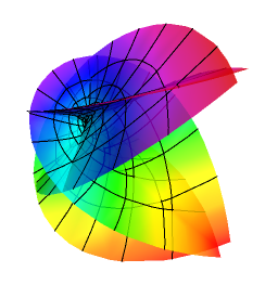
Generating functions f(z)=10z, g(z)=z

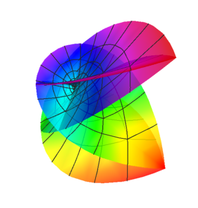
Generating functions f(z)=z, g(z)=10z

Figure 1: Surfaces of type $S$ for different values of $A$ and $C$

Now we are interested whether the functions $f(z)=z$, $g(z)=z+a+i\,b$, $a,\,b\in\mathbb{R}$, define a surface which is really different from $S_{0}$. The chart ${\bf x}(u,v)$ generated by these functions is not in canonical principal parameters so according to Theorem B we change the complex variable $z$ by $(3/2)^{2/3}(i\,z)^{2/3}$. Then the functions

$$\tilde{f}(z)=i\,\left(\frac{3}{2}\right)^{1/3}(i\,z)^{1/3},\quad\tilde{g}(z)=\left(\frac{3}{2}\right)^{2/3}(i\,z)^{2/3}+a+i\,b$$

define a chart ${\bf\tilde{x}}(u,v)$ in canonical principal parameters. Its normal curvature is

$$\tilde{\nu}=\frac{4\left(\frac{2}{3}\right)^{2/3}}{\sqrt{u^{2}+v^{2}}(1+B(u,v)\overline{B}(u,v))^{2}},$$

where $B(u,v)$ is

$$B(u,v)=a+i\,b+\left(\frac{3}{2}\right)^{2/3}(i\,u-v)^{2/3}.$$

Comparing these functions for different values of $(a,b)$ we can say that the resulting surfaces are different. In Figure 2 are shown parts of the surface $S_{0}$, obtained for $(a,b)=(0,0)$ (left), the surface obtained for $(a,b)=(0.5,0)$ (center), and the surface obtained for $(a,b)=(1,0)$ (right).

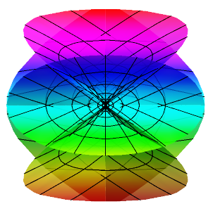
$f(z)=z,\ g(z)=z$

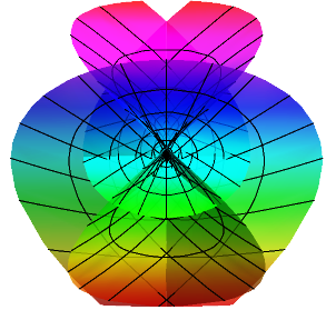
$f(z)=z,\ g(z)=z+1/2$

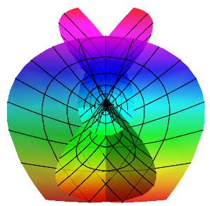
$f(z)=z,\ g(z)=z+1$

Figure 2: Comparison of bi-quartic minimal surfaces for generating functions $f(z)=z$ and $g(z)=z+a+i\,b$

5 Bi-quartic harmonic Bézier  surfaces

We consider bi-quartic tensor product Bézier  surface defined by

$${\bf x}(u,v)=\sum_{i=0}^{4}\sum_{j=0}^{4}{\bf b}_{ij}B_{i}^{4}(u)B_{j}^{4}(v),$$ (10)

where ${\bf b}_{ij},\ i,j=0,\ldots,4$ are the control points of ${\bf x}(u,v)$, and $B_{i}^{4}(u)$ are the Bernstein polynomials of degree $4$ defined for $0\leq u\leq 1$ by

$$B_{i}^{4}(u):=\binom{4}{i}u^{i}(1-u)^{4-i},\qquad\binom{4}{i}=\begin{cases}\frac{4!}{i!(4-i)!},&\text{for }\ i=0,\dots,4,\\ 0,&\text{otherwise.}\end{cases}$$

Recall that if ${\bf x}(u,v)$ is in isothermal parameters then ${\bf x}(u,v)$ is a minimal surface if and only if ${\bf x}(u,v)$ is a harmonic surface, i.e. $\Delta{\bf x}=0$. For a harmonic Bézier  surface Monterde [5] has proved that if we know the control points on two opposite boundaries except one corner point, e.g. nine points $\{{\bf b}_{0j}\}_{j=0}^{4}$ and $\{{\bf b}_{i4}\}_{i=0}^{3}$, then the remaining sixteen control points are fully determined. The proof is based on the harmonic condition $\Delta{\bf x}=0$ which leads to a linear system that has a unique solution.

$\begin{array}[]{ccccc}{\bf b}_{40}&\circ&\circ&\circ&{\bf b}_{44}\\[4.30554pt] {\bf b}_{30}&\circ&\circ&\circ&{\bf b}_{34}\\[4.30554pt] {\bf b}_{20}&\circ&\circ&\circ&\circ\\[4.30554pt] {\bf b}_{10}&\circ&\circ&\circ&{\bf b}_{14}\\[4.30554pt] {\bf b}_{00}&\circ&\circ&\circ&{\bf b}_{04}\end{array}$

Figure 3: Input control points that fully determined bi-quartic harmonic Bézier  surface

Here we assume that nine control points $\{{\bf b}_{i0}\}_{i=0}^{4}$, $\{{\bf b}_{i4}\}_{i=0;i\not=2}^{4}$ as shown on Figure 3 are given. Note that they differ from those used in [5]. In Lemma 1 below we give expressions for the remaining control points through the given points. Then in Proposition 1 we prove that in the case where the given points are symmetric with respect to any of the coordinate planes, then the corresponding harmonic Bézier  surface is symmetric with respect to the same coordinate plane.

Lemma 1

Let nine control points ${\bf b}_{i0},\ i=0,\dots,4$; ${\bf b}_{i4},\ i=0,1,3,4$ be given. A bi-quartic Bézier  surface (10) is harmonic if and only if the remaining sixteen control points satisfy

$$\begin{array}[]{rcl}{\bf b}_{01}&=&(25{\bf b}_{00}+8{\bf b}_{04}-40{\bf b}_{10}-8{\bf b}_{14}+36{\bf b}_{20}-16{\bf b}_{30}+4{\bf b}_{34}+4{\bf b}_{40}-{\bf b}_{44})/12\\ {\bf b}_{41}&=&(4{\bf b}_{00}-{\bf b}_{04}-16{\bf b}_{10}+4{\bf b}_{14}+36{\bf b}_{20}-40{\bf b}_{30}-8{\bf b}_{34}+25{\bf b}_{40}+8{\bf b}_{44})/12\\ {\bf b}_{11}&=&(17{\bf b}_{00}+7{\bf b}_{04}-14{\bf b}_{10}-4{\bf b}_{14}+18{\bf b}_{20}-8{\bf b}_{30}+2{\bf b}_{34}+5{\bf b}_{40}+{\bf b}_{44})/24\\ {\bf b}_{31}&=&(5{\bf b}_{00}+{\bf b}_{04}-8{\bf b}_{10}+2{\bf b}_{14}+18{\bf b}_{20}-14{\bf b}_{30}-4{\bf b}_{34}+17{\bf b}_{40}+7{\bf b}_{44})/24\\ {\bf b}_{02}&=&(13{\bf b}_{00}+8{\bf b}_{04}-28{\bf b}_{10}-8{\bf b}_{14}+30{\bf b}_{20}-16{\bf b}_{30}+4{\bf b}_{34}+4{\bf b}_{40}-{\bf b}_{44})/6\\ {\bf b}_{42}&=&(4{\bf b}_{00}-{\bf b}_{04}-16{\bf b}_{10}+4{\bf b}_{14}+30{\bf b}_{20}-28{\bf b}_{30}-8{\bf b}_{34}+13{\bf b}_{40}+8{\bf b}_{44})/6\\ {\bf b}_{12}&=&(11{\bf b}_{00}+7{\bf b}_{04}-20{\bf b}_{10}-4{\bf b}_{14}+24{\bf b}_{20}-14{\bf b}_{30}+2{\bf b}_{34}+5{\bf b}_{40}+{\bf b}_{44})/12\\ {\bf b}_{32}&=&(5{\bf b}_{00}+{\bf b}_{04}-14{\bf b}_{10}+2{\bf b}_{14}+24{\bf b}_{20}-20{\bf b}_{30}-4{\bf b}_{34}+11{\bf b}_{40}+7{\bf b}_{44})/12\\ {\bf b}_{03}&=&(14{\bf b}_{00}+19{\bf b}_{04}-32{\bf b}_{10}-16{\bf b}_{14}+36{\bf b}_{20}-20{\bf b}_{30}+8{\bf b}_{34}+5{\bf b}_{40}-2{\bf b}_{44})/12\\ {\bf b}_{43}&=&(5{\bf b}_{00}-2{\bf b}_{04}-20{\bf b}_{10}+8{\bf b}_{14}+36{\bf b}_{20}-32{\bf b}_{30}-16{\bf b}_{34}+14{\bf b}_{40}+19{\bf b}_{44})/12\\ {\bf b}_{13}&=&(5{\bf b}_{00}+7{\bf b}_{04}-8{\bf b}_{10}-{\bf b}_{14}+9{\bf b}_{20}-5{\bf b}_{30}+2{\bf b}_{34}+2{\bf b}_{40}+{\bf b}_{44})/12\\ {\bf b}_{33}&=&(2{\bf b}_{00}+{\bf b}_{04}-5{\bf b}_{10}-2{\bf b}_{14}+9{\bf b}_{20}-8{\bf b}_{30}-{\bf b}_{34}+5{\bf b}_{40}+7{\bf b}_{44})/12\\ {\bf b}_{21}&=&(3{\bf b}_{00}+{\bf b}_{04}-4{\bf b}_{10}+8{\bf b}_{20}-4{\bf b}_{30}+3{\bf b}_{40}+{\bf b}_{44})/8\\ {\bf b}_{22}&=&(7{\bf b}_{00}+3{\bf b}_{04}-16{\bf b}_{10}+24{\bf b}_{20}-16{\bf b}_{30}+7{\bf b}_{40}+3{\bf b}_{44})/12\\ {\bf b}_{23}&=&(7{\bf b}_{00}+5{\bf b}_{04}-16{\bf b}_{10}+4{\bf b}_{14}+24{\bf b}_{20}-16{\bf b}_{30}+4{\bf b}_{34}+7{\bf b}_{40}+5{\bf b}_{44})/24\\ {\bf b}_{24}&=&({\bf b}_{00}-{\bf b}_{04}-4{\bf b}_{10}+4{\bf b}_{14}+6{\bf b}_{20}-4{\bf b}_{30}+4{\bf b}_{34}+{\bf b}_{40}-{\bf b}_{44})/6.\end{array}$$ (11)

Proof. It follows straightforward using the corresponding linear system from [5]. $\Box$

Proposition 1

Let the given points ${\bf b}_{i0},\ i=0,\dots,4$; ${\bf b}_{i4},\ i=0,1,3,4$ be symmetric with respect to some of the coordinate planes $Oxy$, $Oxz$, or $Oyz$. Then the corresponding harmonic Bézier  surface defined by Lemma 1 is symmetric with respect to the same plane.

Proof. Let ${\bf b}_{ij}={\bf b}_{ij}(x_{ij},y_{ij},z_{ij})$ and assume that the given control points are symmetric with respect to the plane $Oxy$, i.e. ${\bf b}_{0k}$ and ${\bf b}_{1k}$ are symmetric points to ${\bf b}_{4k}$ and ${\bf b}_{3k}$, respectively, $k=0,4$, and ${\bf b}_{20}$ lies on $Oxy$. Then we have

$$x_{0k}=x_{4k},\ x_{1k}=x_{3k},\ y_{0k}=y_{4k},\ y_{1k}=y_{3k},\ z_{0k}=-z_{4k},\ z_{1k}=-z_{3k}$$ (12)

for $k=0,4$, and $z_{20}=0$. To show that the harmonic Bézier  surface defined by Lemma 1 is symmetric with respect to $Oxy$ it suffices to establish that its control points are symmetric with respect to $Oxy$. We need to establish that (12) holds for $k=1,2,3$ and $z_{2j}=0$ for $j=1,\dots,4$. Next we verify that $x_{01}=x_{41}$, $y_{01}=y_{41}$, $z_{01}=-z_{41}$, and $z_{21}=0$. The analogous relations for the remaining control points follow in a similar way.

From (11) and (12) we have

$$\begin{array}[]{ll}x_{01}&=(25x_{00}+8x_{04}-40x_{10}-8x_{14}+36x_{20}-16x_{30}+4x_{34}+4x_{40}-x_{44})/12\\ &=(29x_{00}+7x_{04}-56x_{10}-4x_{14}+36x_{20})/12=x_{41}.\end{array}$$

Analogous relation holds for $y_{01}$ and $y_{41}$. For the third coordinates $z_{01}$ and $z_{41}$ we obtain

$$z_{01}=(21z_{00}+9z_{04}-24z_{10}-12z_{14})/12=-z_{41}.$$

It remains to show that $z_{21}=0$. We have

$$z_{21} = (3z_{00}+z_{04}-4z_{10}+8z_{20}-4z_{30}+3z_{40}+z_{44})/8$$

$$= \bigl{(}3(z_{00}+z_{40})+(z_{04}+z_{44})-4(z_{10}+z_{30})+8z_{20}\bigr{)}/8=0.$$

The case where the nine given points are symmetric with respect to the other coordinate planes is treated analogously. $\Box$

A bi-quartic harmonic Bézier  surface which is symmetric with respect to $Oxz$ is shown from two different viewpoints in Figure 4. Its control points are presented in Table 1. We note that they are obtained from the minimal bi-quartic Bézier  surface with generating functions $f(z)=z$, $g(z)=z-1$. Hence, the surface in Figure 4 is harmonic minimal Bézier  surface.

$(\frac{512}{3},-\frac{176}{3},\frac{128}{3})$	$(\frac{128}{3},\frac{424}{3},\frac{152}{3})$	$(-128,\frac{128}{3},\frac{32}{3})$	$(-\frac{128}{3},-\frac{296}{3},-\frac{104}{3})$	$(\frac{256}{3},-\frac{80}{3},-\frac{128}{3})$
$(-\frac{64}{3},-\frac{536}{3},-\frac{88}{3})$	$(\frac{224}{3},-\frac{44}{3},\frac{32}{3})$	$(0,0,\frac{8}{3})$	$(\frac{160}{3},-\frac{20}{3},-\frac{32}{3})$	$(\frac{64}{3},\frac{280}{3},\frac{40}{3})$
$(-\frac{512}{3},0,-\frac{160}{3})$	$(0,0,-\frac{8}{3})$	$(-\frac{128}{3},0,0)$	$(0,0,-\frac{8}{3})$	$(-\frac{256}{3},0,32)$
$(-\frac{64}{3},\frac{536}{3},-\frac{88}{3})$	$(\frac{224}{3},\frac{44}{3},\frac{32}{3})$	$(0,0,\frac{8}{3})$	$(\frac{160}{3},\frac{20}{3},-\frac{32}{3})$	$(\frac{64}{3},-\frac{280}{3},\frac{40}{3})$
$(\frac{512}{3},\frac{176}{3},\frac{128}{3})$	$(\frac{128}{3},-\frac{424}{3},\frac{152}{3})$	$(-128,-\frac{128}{3},\frac{32}{3})$	$(-\frac{128}{3},\frac{296}{3},-\frac{104}{3})$	$(\frac{256}{3},\frac{80}{3},-\frac{128}{3})$

Table 1: Control points of a harmonic bi-quartic Bézier  surface that are symmetric with respect to $Oxz$

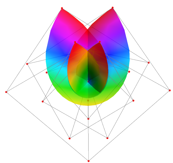
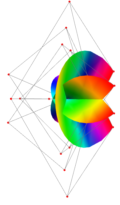
Figure 4: Symmetry of a harmonic bi-quartic Bézier  surface with respect to $Oxz$. The surface is shown from two different viewpoints.

6 Conclusions and Future Work

In this paper we characterize all bi-quartic parametric polynomial minimal surfaces by their generating functions using the Weierstrass formula. We also consider the bi-quartic harmonic Bézier surfaces and establish their symmetry with respect to any of the coordinate planes. We present numerical experiments and give examples. A possible direction for future work is to extend our results for minimal surfaces of higher degrees.

Acknowledgments. This work was partially supported by the Bulgarian National Science Fund under Grant No. DFNI-T01/0001.

Ognian Kassabov
Department of Mathematics and Informatics
University of Transport “Todor Kableshkov”
158 G. Milev Str.
1574 Sofia, BULGARIA
email: okassabov@abv.bg

Krassimira Vlachkova
Faculty of Mathematics and Informatics
Sofia University
5 James Bourchier Blvd.
1164 Sofia, BULGARIA
email: krassivl@fmi.uni-sofia.bg

References

- [1] C. Cosín, and J. Monterde, Bézier surfaces of minimal area, Proc. Int. Conf. of Comput. Sci. ICCS 2002, LNCS 2330, Springer, Berlin Heidelberg, 2002, 72–81.
- [2] G. Ganchev, Canonical Weierstrass representation of minimal surfaces in Euclidean space, arXiv:0802.2374, 2008.
- [3] A. Gray, E. Abbena, and S. Salomon, Modern Differential Geometry of Curves and Surfaces with MATHEMATICA, CRC Press, Boca Raton, 2006.
- [4] O. Kassabov, Transition to Canonical Principal Parameters On Minimal Surfaces, Computer Aided Geometric Design, 31(6), 441–450 (2014).
- [5] J. Monterde, The Plateau-Bézier problem,“Mathematics of Surfaces 2003”, edited by M.J. Wilson, and R.R. Martin, LNCS 2768, Springer, Berlin Heidelberg, 2003, pp. 262–273.
- [6] G. Xu, and G. Wang, Parametric polynomial minimal surfaces of degree six with isothermal parameter, LNCS 4975, Springer, Berlin Heidelberg, 2008, pp. 329–343.
- [7] G. Xu, and G. Wang, Quintic parametric polynomial minimal surfaces and their properties, Differential Geometry and its Applications, 28, 697–704 (2010).
- [8] G. Xu, Y. Zhu, G. Wang, A. Galligo, L. Zhang, and K. Hui, Explicit form of parametric polynomial minimal surfaces with arbitrary degree, Applied Mathematics and Computation, 259, 124-131 (2015).