Computational and in vitro studies of blast-induced blood-brain barrier disruption

Abstract

There is growing concern that blast-exposed individuals are at risk of developing neurological disorders later in life. Therefore, it is important to understand the dynamic properties of blast forces on brain cells, including the endothelial cells that maintain the blood-brain barrier (BBB), which regulates the passage of nutrients into the brain and protects it from toxins in the blood. To better understand the effect of shock waves on the BBB we have investigated an in vitro model in which BBB endothelial cells are grown in transwell vessels and exposed in a shock tube, confirming that BBB integrity is directly related to shock wave intensity. It is difficult to directly measure the forces acting on these cells in the transwell container during the experiments, and so a computational tool has been developed and presented in this paper.

Two-dimensional axisymmetric Euler equations with the Tammann equation of state were used to model the transwell materials, and a high-resolution finite volume method based on Riemann solvers and the Clawpack software was used to solve these equations in a mixed Eulerian/Lagrangian frame. Results indicated that the geometry of the transwell plays a significant role in the observed pressure time series in these experiments. We also found that pressures can fall below vapor pressure due to the interaction of reflecting and diffracting shock waves, suggesting that cavitation bubbles could be a damage mechanism. Computations that include a simulated hydrophone inserted in the transwell suggest that the instrument itself could significantly alter blast wave properties. These findings illustrate the need for further computational modeling studies aimed at understanding possible blast-induced BBB damage.

1 Introduction

Traumatic brain injury (TBI) is the leading cause of death and disability for people under the age of 45 years [105]. Non-penetrating impacts to the head are also associated with increased risk of developing neurologic diseases that include Alzheimer’s disease, Parkinson’s disease, and amyotrophic lateral sclerosis [35, 79, 13, 50]. In addition, repetitive mild traumatic brain injury (mTBI) has been implicated in chronic traumatic encephalopathy [65, 30, 64, 15]. There is also growing evidence that repetitive low intensity non-impact blast wave exposure leads to mTBI, which similar to impact TBI, can initiate slow-developing and potentially permanent brain disturbances [63, 17, 18, 60, 68, 16, 103, 42, 38].

The current and long-term health consequences of TBI and mTBI are of great concern, particularly among military service members and Veterans, as well as civilian noncombatants [2]. Among US and coalition nations’ military service members deployed to Iraq and Afghanistan, it is estimated that approximately 15% to 23% have mTBI [104, 41, 11, 95]. The majority of these mTBIs are blast-related [11, 73, 78, 59, 29], thus motivating the shock tube experiments described in this paper.

Several sophisticated computational efforts (often employing commercial finite element software) have been made in modeling TBI. The majority of these efforts are aimed at modeling the effects of a blast in an idealized human, mouse or rat head [84, 4, 92, 93, 48, 108, 94, 102, 89, 91], sometimes including head-neck interactions [48, 40, 67]. Much of this past work has been recently reviewed in [39].

However, the mechanisms connecting blast wave exposure to mTBI are still not well understood. Clinical diagnostic neuroimaging approaches such as computerized tomography and magnetic resonance imaging (MRI) fail to detect mild injuries. This suggests that the injury mechanisms might occur at very small length scales, even at the scale of a single cell. Several hypothesis have been proposed: the disruption of BBB integrity [88, 43, 76]; cerebral vasospasm mechanotransduced by the blast wave [3]; impairment of axonal functionality [57, 58]; shock wave excitation of phonons that decay into lower frequency oscillations [49] and the formation of cavitating bubbles [71, 67, 66, 80, 109, 74, 37], among others.

In this paper, we study blast-induced BBB using differentiated brain-derived microvessel endothelial cells, considered the biologically most relevant in vitro approach for investigating BBB function [43, 44] (see Appendix for further discussion). Understanding such experiments is important since they isolate one possible cause of TBI — results show that blast functionally disturbs the BBB endothelial cell tight junction protein expression patterns. However, it is still extremely difficult to obtain accurate experimental measurements of the mechanical stresses exerted at the endothelial cells’ location due to blast exposure, which could help relate specific damage mechanisms with experimental outcomes. In order to provide accurate quantitative data on the strength of the shock wave at this location, we developed a computational model which focuses on this particular experimental paradigm.

The primary goal of this work is to computationally model the pressures to which BBB endothelial cells grown in a fluid-filled chamber placed in a shock tube are actually subjected. The results obtained illustrate the fact that the geometry of the chamber plays a large role in this, and suggest the possibility of cavitation occurring in this experimental system. More generally they can aid in interpreting and understanding the experimental results. We also show that the introduction of a hydrophone into the experiment, as might be done in an attempt to measure the pressures experimentally, could itself change the outcome of the experiment and the likelihood of cavitation occurring.

In an in vivo setting, the complexity of skull/bone anatomy, as well as the diffuse anatomy of the microvessel web in the brain, makes computational efforts to model BBB dysfunction extremely challenging. In contrast to this, the simple axisymmetric geometry of the in vitro system facilitates an accurate numerical investigation. As explained further below in detail, this requires novel numerical algorithms to solve compressible Euler equations coupled with a Tammann equation of state (EOS) across interfaces with large jumps in the material parameters at the interface between air and liquid. Numerical and exact methods for Euler equations with a Tammann EOS have been studied and developed previously, e.g. [45, 20, 86, 87, 90] among others; however, to the best of our knowledge, the numerical algorithms developed for this work are the only ones specifically developed to model an experimental setup with fixed sharp interfaces with a big jump in the parameters. We present some description of the methods and a verification study. These methods are studied in more detail in [24, 25] and could be adapted to study related experiments.

1.1 The biological effects of blast exposure on BBB cells

One of the early manifestations of central nervous system (CNS) injury following TBI is BBB disruption [36, 97, 85]. The BBB is responsible for maintaining and regulating separation between the CNS and the circulating peripheral blood supply [8, 110]. In the brain, many cell types work together to regulate the BBB. However, the most important functional components of the BBB are the endothelial cells themselves, which comprise the microvessels that supply the brain. Brain endothelial cells establish specialized connections called tight junctions with other adjoining endothelial cells at points of cell-to-cell contact. This gives rise to an extremely low-permeability cellular barrier that separates the luminal (blood supply) side of the BBB from the abluminal (CNS) side of the BBB. Significantly, there is evidence that BBB disruption may play an important role in the delayed neurologic disorders associated with mTBI [88].

Recent studies have demonstrated that even mild blast exposures are capable of disrupting the BBB [1, 107, 56, 81]. In spite of this important progress, much work remains in order to understand the mechanisms by which mild blast exposure compromises BBB integrity. One approach to address this issue is to study tight junctions using more simplified in vitro models of the BBB [9, 10, 69]. In this experiment, mouse brain-derived endothelial cells (MBECs) were isolated and grown on permeable nylon support membranes, and then incubated in standard cylindrical transwell tissue culture chambers, as illustrated in Figure 1(a). Under these conditions, MBECs form an endothelial cell monolayer with mature tight junctions that functionally mimic the BBB [8, 110]. The cylindrical transwell chamber was then completely filled with tissue culture media, sealed against leaks, placed inside a shock tube, and exposed to the blast, as shown in Figure 1(b). Blast exposure has been shown to impair tight junction integrity under in vitro conditions, as well [43].

Compared to in vivo conditions, in which the BBB is comprised of a highly elaborate matrix of microvessels in the brain, this in vitro BBB system offers a much simpler geometry, with a planar MBEC monolayer positioned uniformly within a defined cylindrical containment vessel (e.g. tissue culture chamber).

Although far removed from an actual brain, this in vitro approach provides the functional and anatomical precision required to correlate computed shock wave dynamics at a specific BBB that has a defined orientation with respect to propagating shock waves. Such combined anatomical and temporal precision is not possible under in vivo experimental conditions. In addition, more complex computational models of the brain cannot directly assess actual BBB biological function.

Importantly, the model presents new computational opportunities to better estimate the biomechanical forces associated with blast overpressure exposure and thereby derive more refined assessments of how forces elicited by blast exposure affect BBB integrity under conditions that are biologically and independently quantifiable.

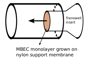
(a) Transwell

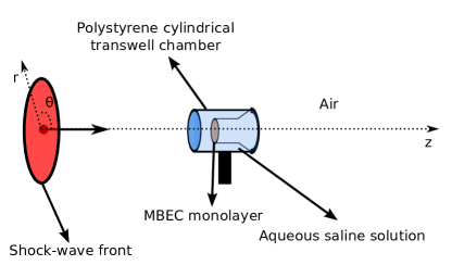
(b) Experimental setup

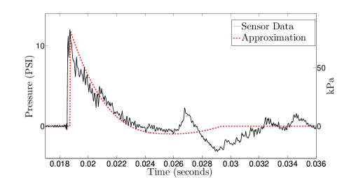
(c) Shock wave profile

(d) 2D axisymmetric model

Fig. 1: (a) Polystyrene transwell chamber illustration. The transwell insert with the MBEC monolayers placed into the chamber filled with an aqueous solution. (b) Cartoon of experimental system, showing the orientation of the transwell in the shock tube. The shock wave travels from the left through the air hitting the polystyrene transwell wall first, then the aqueous saline solution, and finally the endothelial cells sample. (c) The shock wave front profile obtained from a sensor before hitting the transwell as a function of time is shown as the solid line. The approximation to be used as an initial condition in the simulations herein is shown with a dashed line. (d) The 3D axisymmetric shock tube model is obtained by revolving the 2D computational grid. The inside of the inner square corresponds to the cylindrical transwell filled with aqueous saline solution, modeled here as water. The rest of the computational domain is a cylindrical cross section of the shock tube filled with air.

After exposure to the shock wave illustrated in Figure 1(b), tests were performed to measure the integrity of the BBB. The results in Figure 2A demonstrate that increasing blast intensity produced a highly statistically significant decrease in trans-endothelial electrical resistance (TEER) 24 hours post exposure ($p\leq 0.00001$). In addition, there was a statistically significant negative correlation between peak blast intensities (range: 0 – 13.9 psi) and TEER(Pearson $r=-.603$, $p<0.00001$).

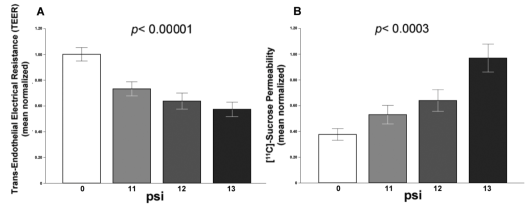
Fig. 2: (A) Trans-endothelial electrical resistance (TEER) was significantly decreased in a blast dose dependent fashion ($p\leq 0.00001$). Histogram denotes mean normalized TEER at 24 hours after a sham exposure (0 psi) ($n$=26) or a single mild blast exposure with a peak amplitude of 11.0-11.9 psi (11), 12.0-12.9 psi (12), or 13.0-13.9 psi (13) ($n=$ 15, 12, and 9, respectively). (B) MBEC monolayer permeability to radioactively labeled [¹⁴C]-sucrose was significantly increased in a blast dose dependent way ($p\leq 0.0003$) with the same blast exposure regimen as in panel A (blast intensity: 0, 11.0-11.9, 12.0-12.9, and 13.0-13.9 psi; $n$ = 7, 4, 3, and 4, respectively). Error bars indicate standard error of the mean (SEM).

In a separate group of MBEC monolayers, we also measured blast-induced leakage of [¹⁴C]-labeled sucrose from the luminal transwell compartment (i.e., peripheral circulating blood supply) into the abluminal transwell compartment (i.e., CNS side). In keeping with the TEER measurements, Figure 2B shows that increasing blast intensity increased MBEC monolayer permeability to [¹¹C]-sucrose ($p\leq 0.0003$). Consistent with this we found a statistically significant correlation between overall peak blast intensities (range: 0–13.9 psi) and [¹⁴C]-sucrose permeability (Pearson $r=.695$, $p<0.001$).

1.2 The computational model

The previous experimental results along with others presented in the Appendix confirm that blast waves produce quantifiable and functional damage to BBB tissue. However, the physical and/or biochemical mechanisms through which blast damages brain tissue is not yet known. In order to gain insight on what some of these mechanisms might be, we have developed a computational model based on the BBB experiment —shown in Figure 1(b) and described in the previous section— that reproduces the dynamics and forces within the transwell chamber. The data computed with our model would be extremely difficult to obtain empirically, and moreover the introduction of a measuring device would affect the outcome of the experiment, as will be explored in detail in Section 2.

The computational model for this particular experiment consists of a rectangular grid modeling the cylindrical axisymmetric cross-section of the shock tube. A rectangular subsection of this grid models the polystyrene cylindrical transwell, filled with saline solution (modeled as water), which is surrounded by air. The setup is shown in Figure 1(b).

Some of the main issues that have been addressed with the computational model presented in the next sections are:

• determine the shock wave interaction with an air-polystyrene-water interface, as in the experiment from Figure 1(b), to verify that the polystyrene layer can be omitted in the computation;

• explore the three-dimensional edge effects of the cylindrical transwell;

• determine whether cavitation may be possible;

• explore how much the insertion of a hydrophone might modify measurements.
  

A necessary first step towards understanding the mechanical response of BBB cells under shock loading is to determine the forces acting on the cells in the laboratory experiments. The shock strength increases as the shock passes from air into the fluid-filled transwell, but the small diameter of the transwell results in waves also propagating in from the sides. When the shock wave hits the distal end of the transwell a reflected rarefaction wave is generated that interacts with the waves from the sides and multiple wave reflections lead to a complex signal.

Moreover, the strong rarefaction waves propagating in the transwell could result in fluid pressure values that are below the vapor pressure, in which case cavitation bubbles may form. As cavitation bubbles collapse they can focus considerable kinetic energy that is capable of disrupting or destroying cellular membranes [72, 19, 106, 12, 37]. Nonetheless, cavitation is a very complicated process that not only depends on the pressure but also on the amount of dissolved gas and other properties of the fluid or tissue. Moreover, cavitation thresholds in the brain are variable and still largely unknown [101, 61, 100, 62]. In this paper, we are only concerned with the possibility of cavitation in the saline solution in the transwell, which was not de-gassed in the experiment reported here.

The computational results obtained in the present paper — although they provide limited answers — support the possibility of collapsing cavitation bubbles as one possible damage mechanism within the experimental arrangement. Note the algorithms and software developed are more widely applicable and could be adapted to study related experiments. For instance, cavitation could perhaps be directly modeled by extending these methods using a six-equation two-phase numerical model instead of Euler equations [75, 87].

In the next section, we will show the results provided by the computational model. In Section 3, we give details of its numerical implementation, followed by further discussion in Section 4.

2 Computational results

We will present the results of the computational version of the experiment shown in Figure 1(b). The setup consists of the polystyrene transwell filled with saline solution, modeled as water, without the endothelial cells, since these are too thin to be included in the model. Nonetheless, we can still measure the pressure intensity as a function of time at the point where the cells are located. We will begin by citing a one-dimensional version of the experiment done in a previous paper [24], where we study the relevance of the thin polystyrene interface separating the air from the saline solution. Afterward, we will explore the full axisymmetric two-dimensional model that will allow us to study the edge effects and possible cavitation. Finally, we repeat this experiment with the addition of an hydrophone-shaped inclusion in order to determine how the inclusion of such a pressure-measuring device might affect the experiment.

2.1 Air-polystyrene-water interface

In a previous work [24], we implemented a one-dimensional version of the experimental system in Figure 1(b) by zooming in on the left face of the transwell chamber. The one-dimensional model consists of only three interfaces: air, polystyrene and water. Since the polystyrene walls of the transwell are very thin relative to the characteristic length of the experiment, we study the effect of decreasing the thickness of the polystyrene layer on the transmitted shock wave. We show that when the polystyrene interface is thin enough in comparison to the transwell length, the results are effectively the same as without it. This result allows us to set up our two-dimensional axisymmetric model with only one fixed interface between air and saline solution and completely neglect the effect of the polystyrene walls. The results and methods from this section are explained in more detail elsewhere [24].

2.2 Two-dimensional axisymmetric results: Cavitation and edge effects

With these simplifications in mind, we constructed the two-dimensional axisymmetric computational model. The implementation was done using the methods of Section 3 to solve the two-dimensional axisymmetric Euler equations (18) coupled with the Tammann equation of state (EOS) (19) to model the different materials. The three-dimensional solution is recovered from revolving the solution on the two-dimensional grid as shown in Figure 1(d), so the model is effectively three-dimensional. The geometry of the air and water interfaces is also shown. The air and water parameters for the Tammann EOS are the ones given in Table 1. Furthermore, to provide an accurate model, we need to model length scales according to the experiment. The cylindrical transwell filled with water (saline solution) is $1.7$ cm long with a radius of $0.85$cm; it can be modeled as a two-dimensional rectangle before being revolved. The shock wave is modeled by feeding the profile shown in Figure 1(c) to the left boundary of the computational domain. However, on the time and length scales of the simulation, we only observe the shock wave and an essentially constant pressure behind the shock, since the rarefaction wave that reduces the pressure behind the shock wave decays over roughly 3 msec while the computation is run for only 134 $\mu$s.

The results from the simulation are shown for different times in Figure 4 as contour and pseudo-color plots of the pressure in the two-dimensional cross section. The corresponding one-dimensional pressure profiles along the axis of rotation are shown in the lower figure of each frame. Several relevant effects can be observed. The amplitude of the pressure is increased as expected from the previous one-dimensional calculations [24]. Also, we can see that the geometry affects the pressure profile as well as the ongoing reflections inside the cylindrical transwell. Of particular interest is the fourth time frame of Figure 4, where the reflected wave has a pressure below water vapor pressure at room temperature. Since the water at room temperature can become gas when the pressure is below the vapor pressure, cavitation is possible. It is known that cavitating bubbles can be responsible for cell detachment and cell membrane poration [72, 19] and could be a possible mechanism of injury to the endothelial cells of the BBB.

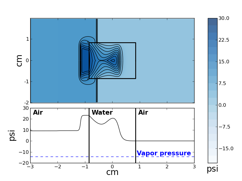
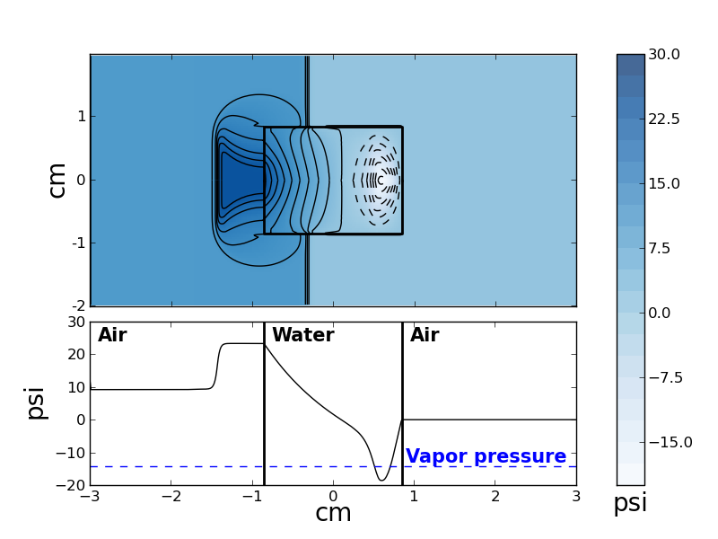
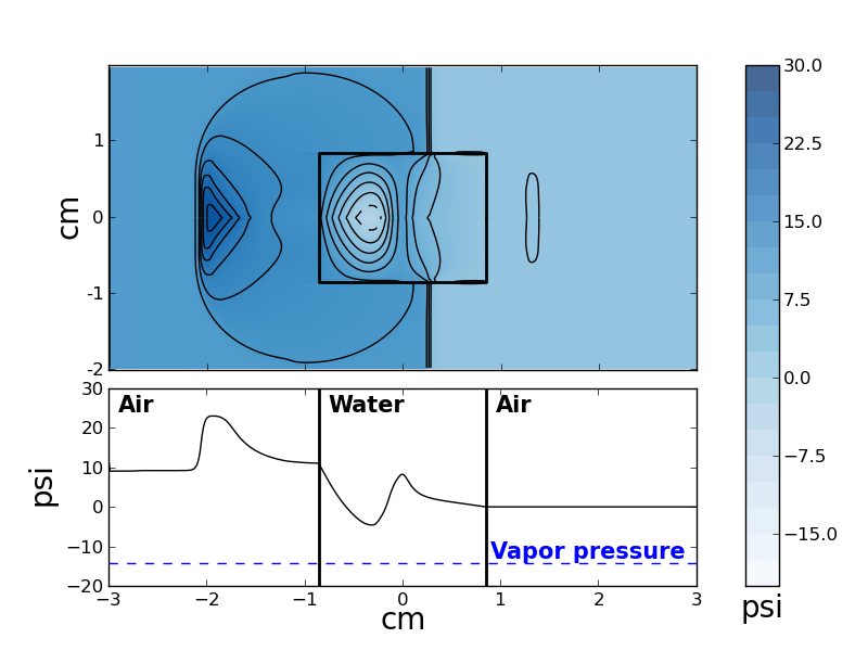
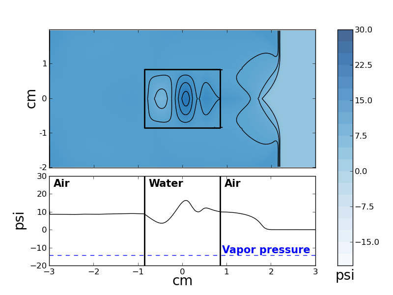
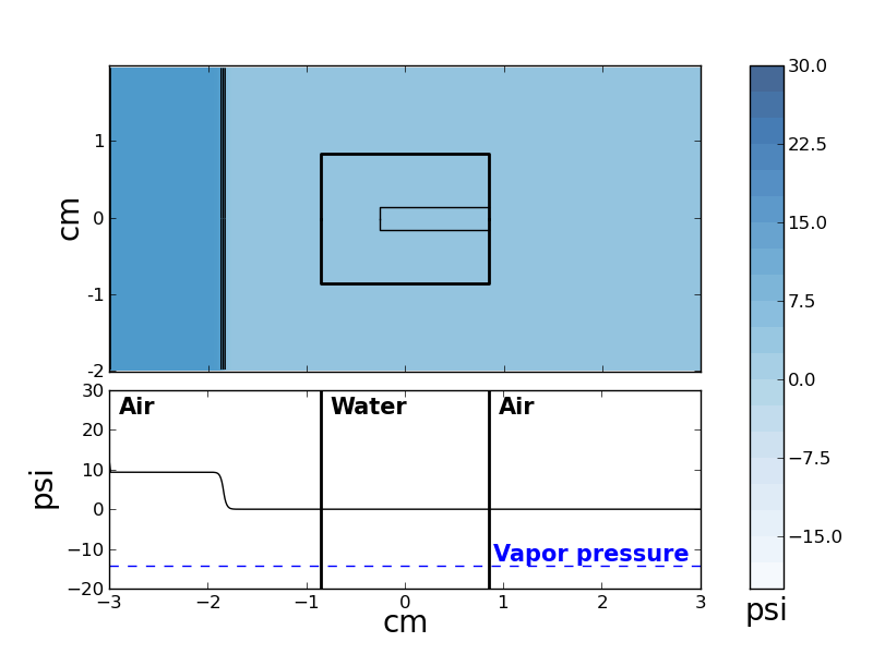
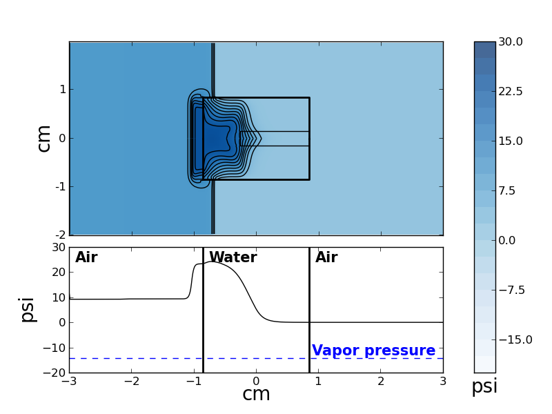
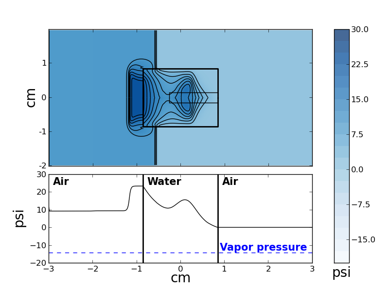
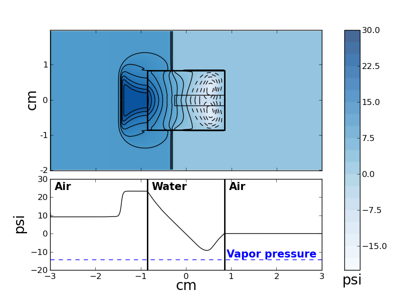
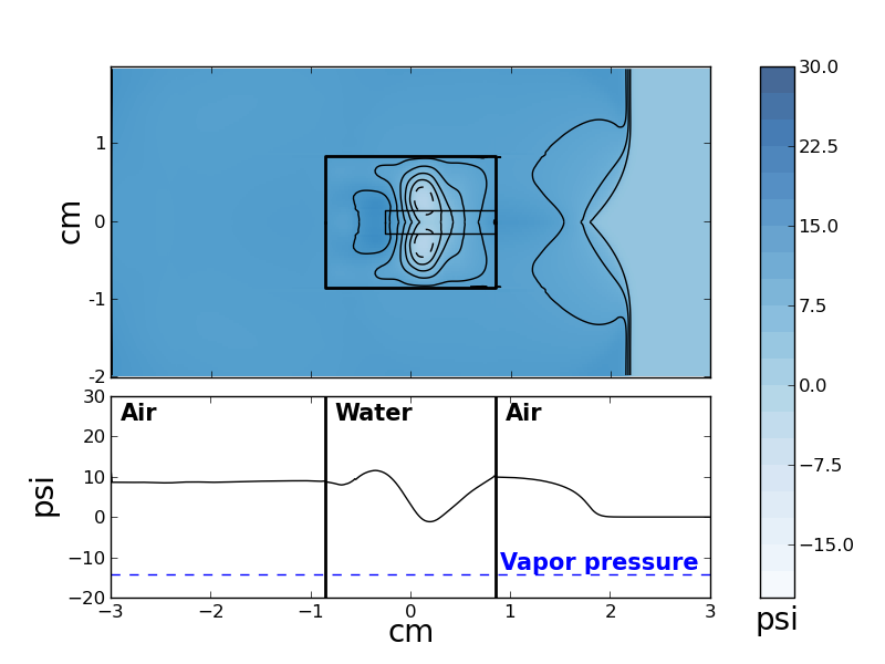
Fig. 3: Axisymmetric simulation output at six different times points $t=30,60,63.2,69.6,84.8,134.4$ $\mu s$. Two-dimensional pressure contour plots of a planar cross section of the cylinder are shown, along with pressure trace along the axis. Water vapor pressure is also shown indicating where cavitation might be possible. Distance is displayed in centimeters and pressure in psi, where atmospheric pressure corresponds to 0 psi.

Fig. 4: Same as Figure 4 but with an hydrophone inserted. Note that in Frame 4 the pressure does not go below the vapor pressure in this case.

To further understand these effects, we can observe Figure 6 where the axisymmetric model is compared to the one-dimensional one. The geometrical edge effects are clearly seen in the second frame, where the pressure profile exhibits a decay in the amplitude after the shock wave has crossed the interface. This is due to the presence of the cylindrical transwell walls parallel to the axis of rotation. As noted elsewhere [24], pressure values below atmospheric pressures do not appear in the one-dimensional case, illustrating that low pressure values that might produce cavitation are a direct consequence of the geometrical edge effects.

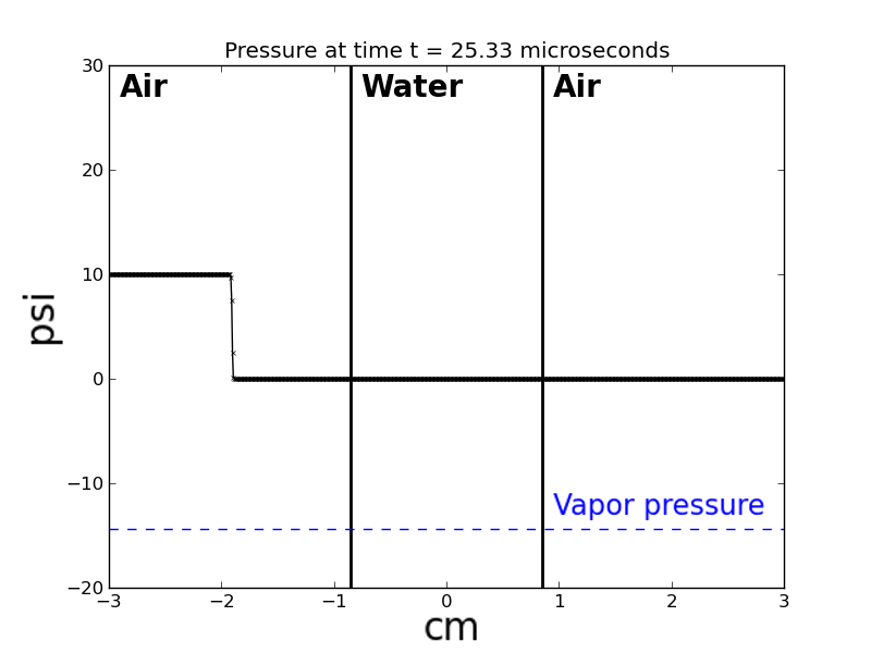
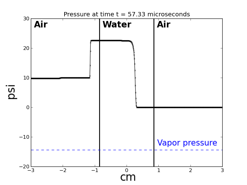
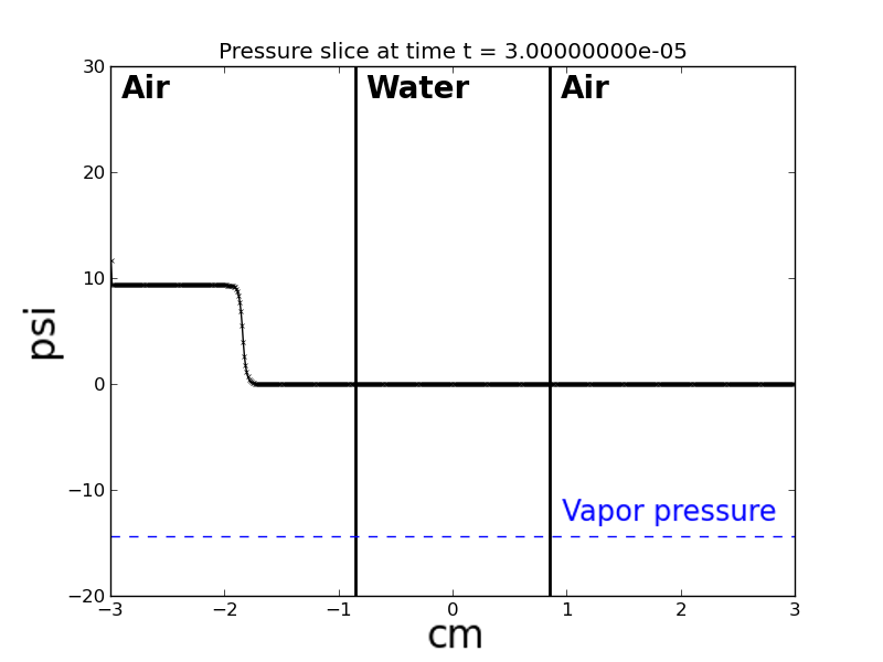
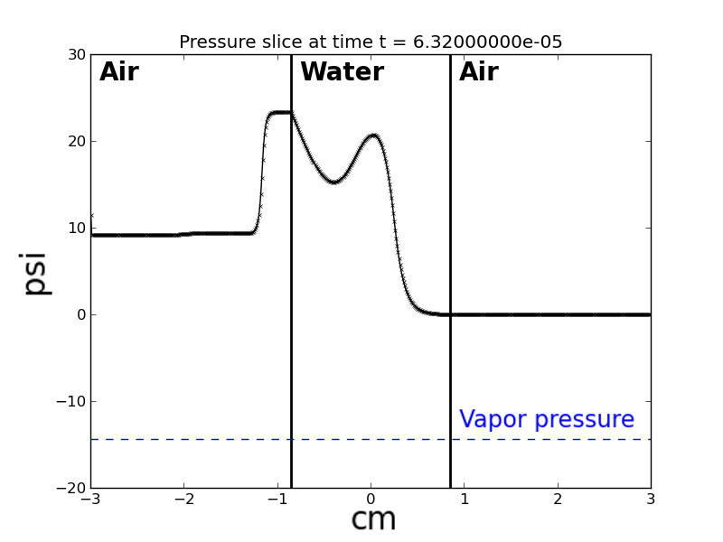
Fig. 5: (a) Pressure shown at two time frames from a one-dimensional simulation. Left: The initial shock approaching the interface. Right: The reflected and transmitted shocks. (b) Pressure along the axis at the same two times, from the two-dimensional axisymmetric simulation. The edge effects in the pressure profile are evident in the second time frame.

Fig. 6: Three-dimensional visualization by revolving the solution of frames 1, 3 and 6 of the two-dimensional axisymmetric results from Figure 4. The cylindrical transwell can be well appreciated on the first frame. The visualization shows the pressure contours, darker contours correspond to higher pressure. Its purpose is to emphasize that the two-dimensional axisymmetric model is effectively modeling three-dimensional wave propagation.

As we mentioned before, we are employing a two-dimensional axisymmetric computational model, which effectively models three-dimensional shock wave propagation. In Figure 6, we show a three-dimensional visualization of the solution by revolving the solution of frames 1,3 and 6 of Figure 4. The figure shows three-dimensional pressure contours, and it is included to emphasize the fact that we are modeling propagation of waves in three dimensions.

2.3 Effects of introducing a hydrophone

One might like to experimentally measure the pressure at the location of the endothelial cells in the transwell in order to determine the force applied to the membrane and the possibility of cavitation. We attempted to introduce a customized version of the Y-104 hydrophone (Sonic Concepts, Bothell WA) in some of our laboratory experiments, but we were unable to gather sufficiently high quality low-frequency data to compare with our numerical results. We did not pursue these experiments because we realized that the introduction of this device could directly affect the signal being measured, reducing the value of such data. A significant advantage of the computational model is that we can measure the pressure at computational gauge locations without interfering with the wave propagation.

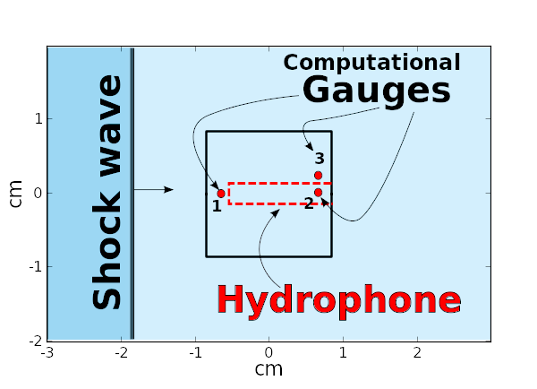
(a) Gauge positions

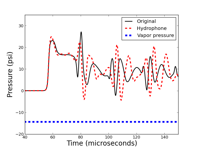
(b) Gauge 1

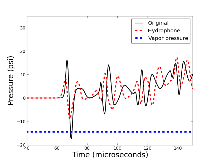
(c) Gauge 2

(d) Gauge 3

Fig. 7: Comparison of the pressure at computational gauges when a hydrophone is introduced with the pressure in the absence of a hydrophone. The location of three gauges is shown on the first frame. The pressure profiles (psi) as a function of time ($\mu$s) are shown for the three gauges. The output of the original simulation without the hydrophone is plotted with a solid line; the output of the simulation with the hydrophone is plotted on a dashed line and the vapor pressure is plotted with a thick dashed line. Note that the pressure falls below vapor pressure in the original simulation at Gauge 2 and Gauge 3 but not when the hydrophone is introduced. Also note that in the presence of the hydrophone, Gauge 2 becomes irrelevant.

We can use the computational model to gain insight on how much the introduction of an hydrophone would change the experimental results. To this end, we include an axisymmetric computational hydrophone down the center of the transwell in the following simulations, with a diameter of 2.85mm to match the Y-104 model. The main effect that concerns us when incorporating the hydrophone in the simulation is the reflection of acoustic waves back into the liquid. The hydrophone is not uniquely composed of a single material and it is designed to have a net impedance of the same order of magnitude as water ($\sim 1.5\times 10^{6}Pa\cdot s/m$). Furthermore, solids usually have impedances higher than water, so we can simply model the hydrophone as a general elastic solid with such properties. For this work, we model it as made of polystyrene with the parameters from Table 1 and a resulting impedance of ($\sim 2.4\times 10^{6}Pa\cdot s/m$). Modifying the impedance of the hydrophone material in the simulations through nine values within the same order of magnitude ($2\times 10^{6}Pa\cdot s/m$ to $7\times 10^{6}Pa\cdot s/m$) did not change any of the qualitative results presented here.

The computational results with the hydrophone are shown in Figure 4. We note there is a significant difference between the results obtained in comparison to those without the hydrophone from Figure 4. These data indicate that, in principle, hydrophone and intracranial pressure sensors placed in a small enclosed volume can alter shock wave propagation in functionally significant ways. This has implications also for rodent experiments, as we see that an intracranial pressure sensor placed within a volume comparable to that of a rodent skull can significantly alter shock wave dynamics, sufficient to change conditions that may favor cavitation.

In order to better quantify the difference between the experiment with and without the hydrophone, we placed three gauges at key points in both systems. In Figure 7, we can observe the comparison between the pressure profile as a function of time in the three chosen points. We can see the pressure only falls below vapor pressure in Gauge 2 and Gauge 3 when the hydrophone is not present. We can conclude that the inclusion of an hydrophone in the experimental system eliminated the possibility of observing cavitation. More importantly, measuring the pressure profile with a hydrophone in an experimental system like this one, affects the observed pressure profile, which supports the use of a computational model for quantifiable insight and answers to some experimental issues.

3 Mathematical and computational models

In this section, we give an outline of the numerical implementation, summarizing the general methods used in Clawpack as well as the original approaches and implementations that were designed uniquely for this work.

3.1 The Euler equations

We use the inviscid Euler equations for compressible flow, with different parameters in the equations of state (EOS) for each material. The axisymmetric Euler equations in cylindrical coordinates ($r$,$\theta$,$z$) take the form

$$\begin{gathered}\frac{\partial}{\partial t}\left[\begin{array}[]{c}\rho\\ \rho u_{r}\\ \rho u_{z}\\ E\end{array}\right]+\frac{\partial}{\partial r}\left[\begin{array}[]{c}\rho u_{r}\\ \rho u_{r}^{2}+p\\ \rho u_{r}u_{z}\\ u_{r}(E+p)\end{array}\right]+\frac{\partial}{\partial z}\left[\begin{array}[]{c}\rho u_{z}\\ \rho u_{r}u_{z}\\ \rho u_{z}^{2}+p\\ u_{z}(E+p)\end{array}\right]=\left[\begin{array}[]{c}-(\rho u_{r})/r\\ -(\rho u_{r}^{2})/r\\ -(\rho u_{r}u_{z})/r\\ -u_{r}(E+p)/r\end{array}\right],\end{gathered}$$ (18)

where $\rho$ is the density; $u_{r}$ and $u_{z}$ denote the velocities in the radial and axial direction, $r$ and $z$ respectively; $E$ is the total energy and $p$ is the pressure. These equations have the same form as the two-dimensional Euler equations with the addition of geometrical source terms (right hand side). These source terms are further discussed in Section 3.4.

For the computational model, we must handle wave propagation in liquid and elastic solids as well as in the air. To handle this range of materials we use the stiffened gas equation of state (SGEOS), also known as the Tammann EOS. This equation of state is very useful to model a wide range of fluids even in the presence of strong shock waves and was successfully used in [31, 32] to model shock wave propagation in tissue and bone. The Tammann EOS is given by

$$p=(\gamma-1)\rho e-\gamma p_{\infty},$$ (19)

where $\gamma$ and $p_{\infty}$ can be determined experimentally for different materials and conditions. The choice of parameters for some materials is shown in Table 1. It is worth mentioning that for sufficiently weak shocks the Tammann EOS can be further simplified to the Tait EOS, which neglects the energy coupling. In [31] this was shown to be adequate for modeling shocks in fluids and solids in the context of shock wave therapy. In this work, we will employ the Tammann EOS since it provides a more comprehensive approach and conserves the energy coupling that could be useful to relate to thermodynamic quantities.

Material	$\gamma$	$p_{\infty}(GPa)$
Air (Ideal gas EOS)	1.4	0.0
Polystyrene	1.1	4.79
Water	7.15	0.3

Table 1: Parameters for the Tammann EOS to model the different materials. The parameters for air and water were taken from [31]. Since the polystyrene is a solid, $\gamma$ was chosen very close to 1, and $p_{\infty}$ was adjusted to yield the right speed of sound in polystyrene. The saline solution in the transwell should have parameters very close to water.

3.2 Numerical methods

The Euler equations (18) are a hyperbolic system of conservation laws, so they can be solved employing finite volume methods (FVM). This is done by using the wave propagation algorithms described in detail elsewhere [54, 53] and implemented in Clawpack [21]. The fundamental problem that needs to be solved at each cell interface of our computation is the well known Riemann problem. A general one-dimensional Riemann problem for a system of conservation laws like Euler equations can be stated as

$$q_{t} +f(q)_{x}=0,$$ (20)

$$q (x,0)=\left\{\begin{array}[]{l l}q_{\ell}&\ \text{if $x<0$}\\ q_{r}&\ \text{if $x>0$},\end{array}\right.$$ (23)

where $q$ is the vector of conserved variables, $f(q)$ the corresponding fluxes and $q_{\ell}$ and $q_{r}$ constant states.

When employing finite volume methods, we need to introduce the concept of cell average: $Q_{i}^{n}=\frac{1}{\Delta x}\int_{x_{i-1/2}}^{x_{i+1/2}}q(x,t_{n})dx$, where $i$ is the cell number and $n$ the time step index. At the edge between two cells, the Riemann problem initial condition would be determined by $q_{\ell}=Q_{i-1}^{n}$ and $q_{r}=Q_{i}^{n}$. After solving the Riemann problems at every cell edge, we can average the respective contributions to obtain the new cells average after a time $\Delta t$. The reader is referred elsewhere [53, 54] for a detailed exposition of the algorithms.

The equations of motion are solved by implementing a hybrid Riemann HLLC-exact Riemann solver for the Euler equations with interfaces. This solver couples a Eulerian HLLC (Harten-Lax-van Leer-Contact) approximate Riemann solver, see [99, 98] to a Lagrangian exact Riemann solver for the Euler equations with a Tammann EOS . As the interfaces are represented by contact discontinuities, the HLLC solver is ideal to deal accurately with interface problems. The method can be extended to two and three dimensions, retaining second order accuracy, by implementing transverse solvers with an unsplit method [53]. We designed the transverse Riemann solvers as approximate solvers based on linear acoustics and adapted them to deal with interfaces. The source terms for the axisymmetric case are resolved using an operator splitting [54, 55]. A detailed description of the hybrid HLLC-exact normal Riemann solver for the Euler equations with the Tammann EOS with discontinuous parameters is presented in [24], in the context of one-dimensional problems. The extension of this solver to a Riemann solver normal to a cell interface in two space dimensions is straightforward and will not be discussed here. For the unsplit wave propagation algorithms implemented in Clawpack, this must be augmented with a transverse Riemann solver, as described in the Section 3.3. The source terms that arise from axisymmetry are handled via a fractional step approach described in Section 3.4.

3.2.1 Verification

In this section, we will verify that the finite volume methods coupled with the hybrid Riemann HLLC-exact Riemann solver for the Euler equations with a Tammann EOS give the correct solution for a simple model problem. As the studies in Section 2 are concerned with the dynamics of a shock wave traveling in an air-water-air system with two interfaces, we use this example as the test case. The exact analytic solutions of Riemann problems for Euler equations are only available in one dimension, so we restrict our verification to a one-dimensional test. This analysis will test the accuracy of the approximate hybrid Riemann solver, the key ingredient of our numerical method, also in the two-dimensional extension of the algorithm.

The test problem is illustrated in the $x$–$t$ plane diagram on the left of Figure 8. We will use a one-dimensional version of our algorithms, where we have an incoming shock of the same shape and intensity than the one used for Figure 4. We divide the domain into three materials: air-water-air, as in the original problem. At the time the shock hits the air-water interface at point A, we can view the problem as a Riemann problem and compare it to the exact solution. Furthermore, after the transmitted shock travels to the second interface, we have a second Riemann problem and can repeat the same procedure at the water-air interface at point B and also compare the transmitted and reflected waves to the exact solution at that point. However, it should be noted that in the numerical algorithm the incoming shock is not perfectly sharp, so we cannot expect a perfect match between our numerical solution and the exact solution.

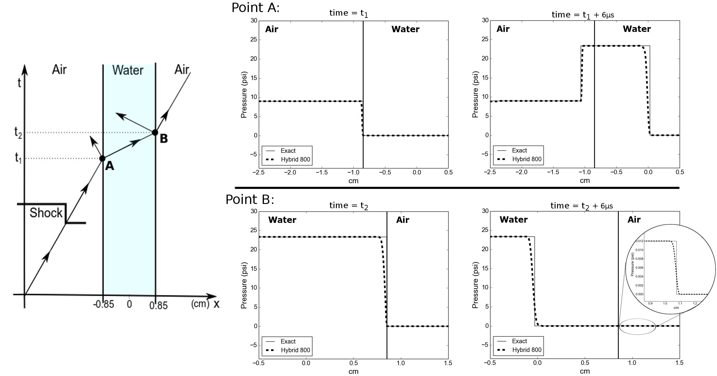
Fig. 8: Verification study of the numerical methods. On the left, we show the $x$–$t$ plane of an incoming shock that hits the air-water interface at point A. The transmitted shock then hits the water-air interface at point B. For both points, we show the solution when the shock hits the interface and another one 6$\mu s$ later. The exact solution can be constructed as described in the text and is compared with the numerical solution computed using the hybrid HLLC-exact solver with 800 grid points. The air and water materials were modeled using the parameters from Table 1.

At point A in Figure 8, we provide two plots: one just before the shock hits the air-water interface at $t_{1}$ where we can frame the problem as a Riemann problem, and the second one 6$\mu s$ later. Both plots show two curves, one using the exact Riemann solver for the Euler equations with the Tammann EOS, with a jump in the parameters [25, 45], and the other one is the numerical solution using the hybrid HLLC-exact solver for the Riemann problems that arise at each cell interface every time step.

The same procedure is repeated in point B of Figure 8. The first plot shows the transmitted shock from the exact Riemann solution at point A, just before hitting the water-air interface at time $t_{2}$, and the second one 6$\mu s$ later. Notice in this last plot that there appears to be no transmitted wave. However, the zoomed-in bubble shows that there is a very weak transmitted shock at this interface of magnitude roughly 0.013 psi. Due to the much lower density of air relative to water, this interface acts nearly like a free boundary and the reflected wave is a rarefaction wave, which is difficult to appreciate from the figure since the difference between the rarefaction head and tail speeds is very small. At both points in Figure 8, we can see a very good agreement between our numerical solution and the exact solution. Furthermore, in Figure 9, we provide a convergence test. We chose to show it using the second plot at point B of Figure 8 since it gathers information of transmitted and reflected waves from both interfaces. Figure 9 shows that the solution converges as we refine the resolution of our numerical solution.

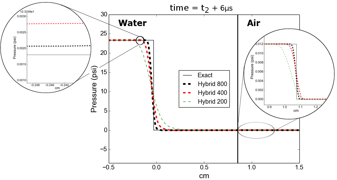
Fig. 9: The last plot in Figure 8 is recomputed with three different numerical resolutions to show convergence. The numerical solutions are computed using the hybrid HLLC-exact solver with 200, 400 and 800 grid points. Two zoomed in regions in key areas are shown.

3.3 Transverse Riemann solvers

In order to obtain second order accuracy and improve stability in two-dimensional hyperbolic problems, the notion of a transverse Riemann solver was introduced in [53]. This solver takes the results of a Riemann solution in the direction normal to a cell interface and splits it into components moving in the transverse direction that contribute to updating the solution in the adjacent rows of grid cells. Other alternatives also exist for solving multi-dimensional conservation laws that attempt to use more fully multi-dimensional Riemann solutions, for example in work of Roe [83] and Fey [33, 34]. Of particular relevance to the approximate Riemann solver approach used here is the work of Balsara [6, 7], who defines two-dimensional HLLC Riemann solvers that accept four input states that come together at an edge and outputs the multi-dimensionally upwinded fluxes in both directions. A comparison between these two approaches could be of relevance in future studies.

For the present problem with sharp interfaces between very different materials, instabilities were seen to easily arise, particularly at the corners of the rectangular region representing the transwell. A special transverse solver was developed that we now describe, based on the solver for acoustics in a heterogeneous media that is described in Section 21.5 of [54]. Note that for two-dimensional problems on rectangular grids, the cell average is calculated as $Q_{i,j}^{n}=\frac{1}{\Delta y\Delta x}\int_{C_{i,j}}q(x,y,t_{n})dxdy$, where $C_{i,j}$ is the cell $[x_{i-1/2},x_{i+1/2}]\times[y_{j-1/2},y_{j+1/2}]$.

We recall the basic idea of a transverse solver in Figure 10. For a constant coefficient linear hyperbolic system of equations $q_{t}+Aq_{x}+Bq_{y}=0$, the jump in normal flux between adjacent cells, $A\Delta Q_{i-1/2}=A(Q_{i,j}-Q_{i-1,j})$, is split via the normal Riemann solver into “fluctuations” $A^{-}\Delta Q_{i-1/2}$ and $A^{+}\Delta Q_{i-1/2}$ that correspond to the net contribution of all left-going or right-going waves to the cell averages on either side. Here $A^{\pm}=R\Lambda^{\pm}R^{-1}$ where $A=R\Lambda R^{-1}$ is the eigen-decomposition of $A$ and $\Lambda^{\pm}$ are the diagonal matrices in which either the negative or positive eigenvalues have been set to zero. Each fluctuation, e.g. $A^{+}\Delta Q_{i-1/2}$, is then further split into down-going and up-going components $B^{-}A^{+}\Delta Q_{i-1/2}$ and $B^{+}A^{+}\Delta Q_{i-1/2}$, based on the matrices $B^{+}$ and $B^{-}$.

In the case of variable coefficients or nonlinear problems, the general notation ${\cal B}^{-}{\cal A}^{+}\Delta Q_{i-1/2}$ and ${\cal B}^{+}{\cal A}^{+}\Delta Q_{i-1/2}$ is used for these two vectors. For variable coefficient acoustics, as described in [54], the up-going fluctuation from the transverse splitting is based on eigenvectors of $B_{ij}$ and $B_{i,j+1}$, while the down-going fluctuation is based on eigenvectors of $B_{ij}$ and $B_{i,j-1}$. For a nonlinear problem $q_{t}+f(q)_{x}+g(q)_{y}=0$, the eigen-decomposition of some averaged Jacobian $g^{\prime}(q)$ is generally used for the transverse Riemann solver.

Fig. 10: Transverse solvers diagram for computational grid cells. The left-going and right going fluctuations of the normal Riemann problem at the edge between grid cells $(i-1,j)$ and $(i,j)$ is shown. The right-going fluctuation $A^{+}\Delta Q_{i-1/2,j}$ is decomposed into the up-going fluctuation $B^{+}A^{+}\Delta Q_{i-1/2,j}$ and the down-going fluctuation $B^{-}A^{+}\Delta Q_{i-1/2,j}$ by employing transverse Riemann solvers.

The present problem involves both nonlinearity and varying material properties. Since we are modeling the almost incompressible liquid in a Lagrangian frame of reference [24], the transverse Riemann problem will mostly be concerned with the two acoustic waves. In order to derive the approximate transverse solver, we will rely on linearized acoustic equations around $\rho_{0},u_{0}$ [54] in terms of the density and momentum,

$$\begin{gathered}\left[\begin{array}[]{c}\rho\\ \rho u\end{array}\right]_{t}+\underbrace{\left[\begin{array}[]{c c}0&1\\ c^{2}&0\end{array}\right]}_{\tilde{B}(Q)}\left[\begin{array}[]{c}\rho\\ \rho u\end{array}\right]_{y}=0,\end{gathered}$$ (31)

where we use $y$ as the space variable to emphasize this is solved in the transverse direction, $c$ is the sound speed and $\tilde{B}(Q)$ can be understood as a lower dimensional approximation of the transverse Jacobian $g^{\prime}(Q_{0})$ for the Euler equations. Note we assumed $u_{0}=0$, which is equivalent to assume we are in a Lagrangian frame of reference. The eigenvectors of the Jacobian of the system are given by $[1,\pm c]$ and the eigenvalues by $\pm c$; however, when solving the transverse Riemann problem, we might have different materials and sound speeds in the cell above or below. Instead of evaluating the whole Jacobian in one state, as in a Roe linear solver [82], we will evaluate the eigenvectors according to their location. These will be given by $v_{U}=[1,c_{U}]$ for the upward acoustic wave and $v_{D}=[1,-c_{D}]$ for the downward acoustic wave with eigenvalues $c_{U}$ and $-c_{D}$. Here $U$ and $D$ refer to cells $(i,j+1)$ and $(i,j)$ when computing ${\cal B}^{+}{\cal A}^{+}\Delta Q_{i-1/2,j}$ and to cells $(i,j)$ and $(i,j-1)$ when computing ${\cal B}^{-}{\cal A}^{+}\Delta Q_{i-1/2,j}$. The matrix of eigenvectors $R$ and its inverse are given by,

$$\begin{gathered}R=\left[\begin{array}[]{c c}1&1\\ c_{U}&-c_{D}\end{array}\right],\end{gathered}\ \ \ R^{-1}=\frac{1}{c_{U}+c_{D}}\left[\begin{array}[]{c c}c_{D}&1\\ c_{U}&-1\end{array}\right].$$

The up-going and down-going fluctuations for ${\cal A}^{+}\Delta Q_{i-1/2,j}$ are obtained by expanding the fluctuation in terms of these two eigenvectors or waves, ${\cal A}^{+}\Delta Q_{i-1/2,j}=\alpha_{U}v_{U}+\alpha_{D}v_{D}$, so we need to solve $R\alpha={\cal A}^{+}\Delta Q_{i-1/2,j}$, Note that the required fluctuation ${\cal A}^{+}\Delta Q_{i-1/2,j}$ for the Euler equations is a 4 dimensional vector with fluctuations in density, normal momentum, transverse momentum and internal energy. As we are only interested in the acoustic waves, we will assume the fluctuations in normal momentum and energy are negligible, so we define the acoustic part of the fluctuation as the first and third entry of the 4 dimensional vector, i.e. ${\cal A}^{+}_{ac}\Delta Q_{i-1/2,j}=[{\cal A}^{+}_{\Delta Q1},{\cal A}^{+}_{\Delta Q3}]$. Solving the system for the vector $\alpha=R^{-1}{\cal A}^{+}_{ac}\Delta Q_{i-1/2,j}$, we obtain

$$\alpha_{U}=\frac{1}{c_{U}+c_{D}}\left(c_{D}{\cal A}^{+}_{\Delta Q1}+{\cal A}^{+}_{\Delta Q3}\right),$$

$$\alpha_{D}=\frac{1}{c_{U}+c_{D}}\left(c_{U}{\cal A}^{+}_{\Delta Q1}-{\cal A}^{+}_{\Delta Q3}\right).$$

The up-going and down-going acoustic fluctuations are given by the velocity times the waves,

$${\cal B}^{+}_{ac}{\cal A}^{+}\Delta Q_{i-1/2,j}=c_{U}\alpha_{U}v_{U},$$

$${\cal B}^{-}_{ac}{\cal A}^{+}\Delta Q_{i-1/2,j}=-c_{D}\alpha_{D}v_{D}.$$

We require to solve two of these transverse solvers for the Euler equations as shown in the grid in Figure 10. We will only consider the up-going fluctuation of the transverse solver at $(i,j+1/2)$ and the down-going fluctuaction of the solver at $i,j-1/2$. This yields the full fluctuations as

$$\begin{gathered}{\cal B}^{+}{\cal A}^{+}\Delta Q_{i-1/2,j}=\frac{c_{3}\left(c_{2}{\cal A}^{+}_{\Delta Q1}+{\cal A}^{+}_{\Delta Q3}\right)}{c_{3}+c_{2}}\left[\begin{array}[]{c}1\\ 0\\ c_{3}\\ 0\end{array}\right],\\ {\cal B}^{-}{\cal A}^{+}\Delta Q_{i-1/2,j}=\frac{-c_{1}\left(c_{2}{\cal A}^{+}_{\Delta Q1}-{\cal A}^{+}_{\Delta Q3}\right)}{c_{1}+c_{2}}\left[\begin{array}[]{c}1\\ 0\\ -c_{1}\\ 0\end{array}\right],\end{gathered}$$

where $c_{1},c_{2}$ and $c_{3}$ are the speeds of sound in cells $(i,j-1)$, $(i,j)$ and $(i,j+1)$ respectively and the non-acoustic fluctuations were neglected. The sound speeds are calculated with the pressure, density and the parameters of the Tammann EOS in the respective cell with $c=\sqrt{\gamma\frac{p+p_{\infty}}{\rho}}$. Note this process is repeated in exactly the same manner for the left going fluctuation ${\cal A}^{-}\Delta Q_{i-1/2,j}$ of the normal Riemann problem.

3.4 Geometrical source terms

In order to solve for the source terms of equation (18), we need to apply a splitting method, see [54]. In the first half time step, we solve the homogeneous version of equation (18) over the whole grid, and in the second step we solve the system of ODEs obtained by ignoring the flux terms,

$$\begin{gathered}\frac{d}{dt}\left[\begin{array}[]{c}\rho\\ \rho u_{r}\\ \rho u_{z}\\ E\end{array}\right]=\left[\begin{array}[]{c}-(\rho u_{r})/r\\ -(\rho u_{r}^{2})/r\\ -(\rho u_{r}u_{z})/r\\ -u_{r}(E+p)/r\end{array}\right].\end{gathered}$$ (41)

This equation can be solved with any explicit time integrator method like forward Euler and Runge-Kutta methods or an implicit solver, such as TR-BDF2. However, this particular system can be solved exactly. Consider the first equation of equations (41) and multiply it by $u_{r}$, then

$$u_{r}\frac{d\rho}{dt} =\frac{\rho u_{r}^{2}}{r},$$

$$\Rightarrow\frac{d\rho u_{r}}{dt}-\frac{du_{r}}{dt}\rho =-(\rho u_{r}^{2})/r,$$

where we used the product rule. Now substituting the second equation of (41) into this result, we obtain $\frac{du_{r}}{dt}=0$, so $u_{r}$ is constant. The same procedure can be applied to obtain that $u_{z}$ is also constant.

As the total energy is given by $E=\rho e+\frac{1}{2}\rho(u_{r}^{2}+u_{z}^{2})$, where the Tammann EOS (19) allows the substitution $\rho e=(p+\gamma p_{\infty})/(\gamma-1)$. As $u_{r}$ and $u_{z}$ are constant, we can differente the energy, $E_{t}=(\rho e)_{t}=\frac{1}{\gamma-1}p_{t}$. These results in conjuction with the fourth equation of (41), yield $p_{t}=-(u_{r}/r)[\gamma(p+p_{\infty})+\frac{1}{2}(\gamma-1)\rho(u_{r}^{2}+u_{z}^{2})]$. We now have a full system of equations in the primitive variables:

$$\frac{d\rho}{dt} =-(u_{r}/r)\rho,\ \ \ \ \frac{du_{r}}{dt}=0,\ \ \ \ \frac{du_{z}}{dt}=0,$$

$$\frac{dp}{dt} =-(u_{r}/r)\left(\gamma(p+p_{\infty})+\frac{1}{2}(\gamma-1)\rho(u_{r}^{2}+u_{z}^{2})\right).$$

The first three equations can easily be solved, and the fourth equation can also be solved with the solution of the first one and an integrating factor. Using the fact that the initial conditions for the computation are the variables at time $t^{n}$, and we want the solution at time $t^{n+1}=t^{n}+\Delta t$, we obtain

$$\begin{split}\rho^{n+1}&=\exp\left(-\frac{\Delta tu_{r}^{n}}{r}\right)\rho^{n},\ \ \ \ u_{r}^{n+1}=u_{r}^{n},\ \ \ \ u_{z}^{n+1}=u_{z}^{n},\\ p^{n+1}&=\exp\left(-\frac{\Delta t\gamma u_{r}^{n}}{r}\right)p^{n}-p_{\infty}\left(1-\exp\left(-\frac{\Delta t\gamma u_{r}^{n}}{r}\right)\right)\\ &\ \ \ -\frac{\rho^{n}}{2}\left((u_{r}^{n})^{2}+(u_{z}^{n})^{2}\right)\left[\exp\left(-\frac{\Delta tu_{r}^{n}}{r}\right)-\exp\left(-\frac{\Delta t\gamma u_{r}^{n}}{r}\right)\right],\\ E^{n+1}&=\frac{p^{n+1}+\gamma p_{\infty}}{\gamma-1}+\frac{1}{2}\rho^{n+1}\left((u_{r}^{n})^{2}+(u_{z}^{n})^{2}\right).\end{split}$$ (42)

The parameters $\gamma$ and $p_{\infty}$ are given by the Tammann EOS in equation (19). The equations we just obtained allow us to calculate one-time step of (18) in our splitting method. Note these source terms are never singular in the computation; when using finite volume methods, the quantities are evaluated at cell centers, so $r>0$.

4 Discussion

A computational model was designed to better understand the physical forces developed by blast-induced shock waves that can damage brain endothelial cells in an in vitro model of the BBB. The numerical modeling of the experiment employs finite volume methods and requires coupling a highly compressible material (air) with a nearly incompressible liquid contained in a fixed region in space. The coupling is accomplished by employing a Tammann EOS and designing both normal and transverse Riemann solvers that can couple these two materials — one in a Eulerian frame of reference and the other in a Lagrangian frame of reference. Results show the shock wave pressure amplitude and velocity increase when crossing from air to the water (saline solution). This is in agreement with the one-dimensional simulations described by us previously [24], as well as other works mentioned in a recent review [39]. One aspect of the potential relevance of this effect lies in the underestimation of the pressure intensities experienced by the cells when one considers only the amplitude and kinetic properties of a standard open field blast overpressure.

Comparison of the computational results here to the one-dimensional tests performed in [24] show that the transwell geometry is very relevant. The edge effects from the cylinder, combined with the rarefaction wave arising when the shock reflects off the distal end of the transwell, can generate low enough pressure to potentially produce cavitation, which could be a cause of cell damage [72]. The simulation with a hydrophone in place does not show low enough pressure values to produce cavitating bubbles. These results indicate that the computational model could be useful to experimentalists in analyzing how the introduction of a measuring device affects the outcome of the experiment and the likelihood of cavitation being a BBB tissue damage mechanism.

Although based on an idealized model, our computational approach allows us to measure the pressure profile at any point and at the exact location of the biological sample without interfering with the actual experimental setup. This task would be extremely difficult to obtain empirically. The high-resolution signal obtained by our computational method allows us to apply it to identify regions with low enough pressure to potentially produce cavitation. Furthermore, our results allow us to suggest cavitation as a damage mechanism that might explain the experimental results, for instance, the mislocalization of the tight junction proteins, ZO1, and claudin-5, that functionally disturb the BBB. This kind of study can clarify the qualitative behavior of the system and, where it is impossible for experimentalists. It can also suggest possible connections between damage mechanisms and anatomical, functional, morphological, and molecular specificity, obtained from the experimental results.

The computational model developed in this work was designed for a specific application; however, the methods developed can be adapted and applied to other experiments with similar simplified geometry. These methods can also be extended to other geometries and the Clawpack software (with adaptive mesh refinement) can be applied in situations where a logically rectangular grid can be mapped to a quadrilateral two-dimensional grid. This can include situations in which the interface is circular or of other smooth shape lacking corners using the sort of mappings proposed in [14], which have been used for elastic and poroelastic wave propagation problems in the work of Lemoine [51, 52]. Extension of the methods proposed in this paper to such cases is currently under way and will be reported elsewhere [25]. This extension is clinically relevant; it allows detailed studies of the pressure signal obtained by shock waves interacting directly with the skull in conditions that might not be feasible experimentally, emphasizing the importance of having a computational model available.

The computational simulations were evaluated up through the first 200 microseconds. As seen in Figure 1(c), this corresponds to a very short time period behind the shock, before the bulk of the trailing rarefaction wave has passed the transwell. Planned future work includes the refinement of our numerical method to carry out the simulation to longer times. This can be of relevance given the negative pressure values and oscillations that arise on millisecond time scales, as well as the secondary reflection-induced shock, see Figure 1(c). These features, along with the internal reflections might also cause or even increase cavitation effects.

Some other possible future research directions include extension of the computational methods to arbitrary interface geometry and to two-phase models that can simulate cavitation. In addition, the in vitro system coupled with the computational model can be used for future clinically relevant studies. The ability to determine pressure traces at the precise location of the planar endothelial cell monolayer could be used as an input into a mechanical model of membrane dynamics during blast wave propagation. This would permit new and highly refined estimates of the physical forces that brain endothelial cells may be exposed to, such as high frequency BBB oscillations that may disrupt cellular functions even without gross brain displacements.

An important novel aspect of this approach is that these estimates can be correlated to specific quantifiable measurements of cellular damage, dysfunction of the BBB as a system of interacting cells, and even aberrant subcellular protein trafficking where it is possible to investigate the mechanisms by which blast alters how critical BBB proteins, such as claudin-5 (Appendix, Figure 5.2) are misdirected inside cells away from tight junctions.

The simulation code developed in this work is available at [26], along with the raw data and SPSS statistical analysis discussed below in Section 5.4. The simulation code relies on Clawpack [21] and the results presented in the paper were obtained with Version 5.2.2.

5 Appendix: Additional experimental results and methodology

Using well-established methods [9, 10, 69] mouse brain-derived endothelial cells (MBECs), purified from wild-type C57BL6 mice, were grown on permeable nylon support membranes in standard transwell chambers (see Figure 1(a)) and formed endothelial cell monolayer tight junctions that functionally mimic the BBB, which is responsible for maintaining and regulating separation between the central nervous system (CNS) and the circulating peripheral blood supply [8, 110]. The transwell chambers were filled completely with an aqueous solution (serum-free DMEM/F12 medium containing bFGF (1 ng/ml) and hydrocortisone (500 nM)). For blast exposure, the transwells were secured in the shock tube with the bottom of the transwell facing the oncoming shock wave (see Figure 1.2). For all experiments, BBB cells were exposed to a single mild blast of indicated intensity (psi).

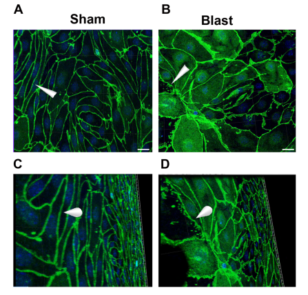
Fig. 11: (A) Laser confocal microscopy reveals normal ZO-1 expression patterns expressed specifically at uniform, well-defined tight junctions along cell-to-cell interfaces within the plane of the brain-derived microvessel endothelial cell monolayer. (B) In contrast to the sham condition, ZO-1 expression in blast-exposed endothelial cells is highly dystrophic with widespread mislocalization in cellular domains remote from tight junctions. Panels A and B show a merged, serial reconstruction comprised of 27 images acquired at $0.2\mu$m intervals along the z-axis orthogonal to the plane parallel with the MBEC cell monolayer. (C and D) Lower panels show oblique x-y-z plane views of the panels above (A,B), thereby permitting an improved assessment of blast-induced tight junction dysmorphology compared to normal sham tight junctions. Nuclei are stained blue with Dapi. Arrowheads denote the same cell-to-cell contact domains in the corresponding sham (A, C) and blast (B, D) images. Scale bars = $20\mu$m.

In addition to the experiment presented in Section 1.1, we performed another experiment to investigate the effects of the shock tube blast exposure on tight junction morphology. Singly blasted (13-13.9 psi) or sham-treated monolayers were immunostained with antibodies recognizing the tight junction-associated scaffolding protein, ZO-1 [96] 24 hours after treatment and then imaged using laser confocal microscopy. ZO-1 expression in sham-treated MBEC monolayers appeared morphologically normal with ZO-1 immunostaining tightly restricted to the interposing plasma membrane domains at points of cell-to-cell contact (Figure 11A). In marked contrast to this, blast exposure induced ragged, hypertrophic appearing tight junctions (Figure 11B). In addition, ZO-1 expression appeared mislocalized in association with peri- abluminal and/or peri-luminal plasma membranes domains. This expression pattern is also consistent with diffuse intracellular cytoplasmic ZO-1 mislocalization.

The confocal images in Figure 11A and Figure 11B are maximum-field projections comprised of 27 merged images collected at $0.2\mu$m step intervals in the z-axis orthogonal to the plane of the MBEC monolayer, thereby representing a total depth of $5.4\mu$m that encompassed the full cross-sectional width of the MBEC monolayers. Figure 11C and Figure 11D depict three-dimensional serial reconstructions of images in the upper panels projected at oblique angles. For ease of reference, the arrowheads denote the same cell-to-cell contact points in panels A, C and B, D (sham and blast-exposed, respectively). From these oblique angles the degree of blast-induced tight junction dysmorphology and ZO-1 mislocalization are more easily appreciated (Also, see supplementary videos).

Claudin-5 is a tight junction-specific membrane bound protein [47] that is a critical regulator of BBB permeability [70]. Figure 12 shows that a single mild blast exposure also markedly disrupted claudin-5 expression. As with Z0-1, claudin-5 immunostaining revealed aberrant, hypertrophic appearing tight junctions in the blast-exposed monolayers. In addition, the asymmetric peri-nuclear claudin-5 immunostaining clearly demonstrates that blast exposure caused it to become aberrantly retained within the cells, thus raising the possibility that normal polarized subcellular trafficking of claudin-5 into and/or away from tight junction domains may be disrupted in the blast-exposed MBECs.

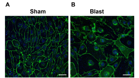
Fig. 12: (A) Laser confocal microscopy reveals normal claudin-5 expression at tight junctions localized along cell-to-cell contacts of the MBEC monolayer. (B) In contrast to the sham controls, claudin-5 expression in blast-exposed endothelial cells is dysmorphic, indicative of aberrant tight junction structure. In addition, claudin-5 is broadly mislocalized and accumulates in asymmetric peri-nuclear intracellular compartments, strongly suggesting that blast exposure induces aberrant subcellular trafficking of claudin-5. Nuclei are stained blue with Dapi. Scale bars = $25\mu$m.

These data suggest that blast exposure causes mislocalization of the tight junction proteins, ZO1 and claudin-5, away from tight junctions. Previous work using the continuous cell line, bEnd.3 showed that blast causes a loss of ZO1 and claudin-5 [43, 44]. This difference could be because bEnd.3 cells are less differentiated than brain-derived microvessel endothelial cells, and which form barriers with lower TEER values than primary brain endothelial cultures used in this report [27]. Nonetheless, our findings in BMECs and in vitro blast studies using bEnd.3 cells [43, 44], collectively demonstrate that blast exposure disturbs expression of proteins critical for maintaining BBB integrity.

Mechanistically, protein mislocalization suggests a dynamic alteration in the cellular process of adjusting to injury, whereas overall tight junction protein loss may suggest co-attending endothelial cell death or impaired protein production or increased tight junction proteolysis. Increasingly, tight junction protein mislocalization is viewed as an underlying pathology in diseases with BBB disruption and is the pattern, for example, in inflammatory conditions [28, 5].

5.1 Culture of primary brain microvascular endothelial cells

Brain microvascular endothelial cells (BMECs) were isolated from 6-8 week old CD-1 mice based on established standard with some modifications procedures [22, 46]. All procedures involving animal subjects were carried out following protocols approved by the Veterans Affairs Puget Sound Health Care System Institution Animal Use and Care Committee (IACUC). Briefly, meninges were removed from freshly dissected brain cortices, and then the brain was minced. The minced brain matter was ground using a Dounce homogenizer in Dulbecco’s Modified Eagle’s Medium/Nutrient Mixture F-12 Ham (DMEM/F12; Sigma-Aldrich) supplemented with gentamicin ($50\mu g/ml$; Sigma-Aldrich). 30% Dextran (v/v; from Leuconostoc spp., MW  70,000 Da; Sigma-Aldrich) was added to the homogenate 1:1 and supplemented with 10% bovine serum albumin (BSA, Sigma-Aldrich) to achieve a final concentration of 0.1%. The mixture was centrifuged at 3000 × g for 25 $\mathrm{min}$ at $4\celsius$. The pellet obtained after the centrifugation was re-suspended in DMEM/F12, filtered through a $70\mu m$ nylon mesh, and centrifuged again at 1000 × g for 10 $\mathrm{min}$ at room temperature (RT). The resulting pellet was digested at $37\celsius$ for 30 $\mathrm{min}$ with DMEM/F12 containing collagenase (0.2 U/ml), dispase (1.6 U/ml; collagenase/dispase, Roche Life Sciences) and DNase I ($10\mu g/ml$; Sigma-Aldrich). The digested vessel suspension was filtered through a $21\mu m$ nylon mesh. The filtrate was washed several times with DMEM/F12, and the resulting capillary suspension was seeded on dishes coated with collagen type IV (0.1 mg/ml; Sigma-Aldrich) and fibronectin (0.1 mg/ml; Sigma-Aldrich). BMECs were cultured in BMEC medium, consisting of DMEM/F12 supplemented with 20% plasma-derived fetal bovine serum (Animal Technologies), 1% GlutaMAX (Life Technologies), basic fibroblast growth factor (bFGF, 1 ng/ml; Roche Life Sciences), heparin ($100\mu g/ml$), insulin ($5\mu g/ml$), transferrin ($5\mu g/ml$), selenium (5 ng/ml) (Insulin-transferrin-selenium medium supplement; Life Technologies), and gentamicin ($50\mu g/ml$; Sigma-Aldrich. Puromycin (4 $\mu$g/ml; Sigma-Aldrich) was added to BMEC medium for the first 48 hours after plating to remove pericytes and increase endothelial cell purity [77]. Cultures were maintained at $37\celsius$ in a humidified atmosphere of 5% CO₂ / 95% air. The medium was changed 24 hours after plating to remove non-adherent cells, red blood cells, and debris. At 48 hours after plating, the medium was changed again with new medium containing all the components listed above, except puromycin. The purified primary BMECs were used to construct in-vitro models when 80% confluent (typically the 5th day after isolation).

5.2 Construction of the in-vitro blood-brain barrier model

Monolayers of brain microvascular endothelial cells were used for all experiments. Endothelial cells were briefly treated with 0.25% Trypsin-EDTA (Sigma-Aldrich) and seeded on the inside of a fibronectin-collagen type IV (0.1 mg/ml, each) coated polyester membrane ($0.33cm^{2},0.4\mu m$ pore size) of a transwell-clear insert (Corning, Tewksbury MA) at a density of $4\times 104$ cells per well. The medium used to plate the cells each of the transwells fitted to a 24-well plate contained all the components of BMEC medium, listed above, with the addition of hydrocortisone ($500nM$; Sigma-Aldrich). The medium in the luminal chamber was changed 24 hours after seeding. BMEC monolayers were cultured for 3 days before use in blast experiments. Transendothelial electrical resistance (TEER, in $\Omega\times cm^{2}$) was measured using an ohmmeter equipped with an STX-2 electrode (World Precision Instruments; Sarasota, FL). The TEER of cell-free transwell-clear inserts was subtracted from obtained values. TEER was measured immediately prior to blast exposure and 24 hours post-exposure.

5.3 Exposure of BMEC to Blast

Transwells were placed into the blasting apparatus, consisting of a modified 24-well plate configuration containing only 4 wells of the 24-well plates with a rubber gasket fitted to the modified plate. The medium was discarded from the luminal side of the transwell inserts and the inserts were placed in the middle two chambers of the blasting apparatus. The wells were filled completely with serum-free DMEM/F12 medium containing bFGF (1 ng/ml) and hydrocortisone (500 nM). A rubber gasket was placed between the filled wells and the lid of the apparatus to completely seal the chambers without air bubbles. The treatment apparatus (a single row of 4 transwell chambers with the two chambers in the middle containing the membrane inserts with BMECs) was then taped firmly to a rigid steel frame with 1/4 inch wire mesh, mounted in the blast tube, and exposed to a single mild blast (range: $11.0$ to $13.9$ peak $\mathrm{psi}$). Non-blasted sham controls were prepared and processed as above but were not exposed to a blast. Following treatment (blast or sham), the medium was aspirated from the chambers. The inserts were placed in a 24-well plate with fresh serum-free medium and returned to $37\celsius$ in a humidified atmosphere of $5\%$ CO${}_{2}/95\%$ air.

5.4 Transendothelial permeability

Permeability to [14C]-sucrose was measured 24 hours after exposure to blast. Transwell inserts were first washed with physiological buffer containing $1\%$ bovine serum albumin ($141mM$ NaCl, $4.0mM$ KCl, $2.8mM$ CaCl₂, $1.0mM$ MgSO₄, $1.0mM$ NaH₂PO₄, $10mM$ HEPES, $10mM$ D-glucose and $1\%$ BSA, pH $7.4$). The inserts were placed in a new 24-well plate containing $600\mu l$ physiological buffer with $1\%$ BSA in the abluminal chamber. To initiate permeability experiments, [14C]-sucrose ($150,000cpm/well$) in physiological buffer with $1\%$ BSA was added to the luminal chamber and $500\mu l$ samples were collected from the abluminal chamber at 10, 20, 30, and 45 $\mathrm{min}$. When samples were removed from the abluminal chamber, an equal volume of fresh $1\%$ BSA/physiological buffer was immediately added to the abluminal chamber to replace the sample volume. Liquid scintillation fluid was added to each sample and the radioactivity was measured using a liquid scintillation counter. The permeability coefficient and clearance of [¹⁴C]-sucrose was calculated according to previously published methods [23]. Clearance was expressed as microliters of radioactive tracer diffusing from the luminal to the abluminal chamber, and it was calculated using the initial amount of radioactivity in the loading chamber and the measured amount of radioactivity in the collected samples. Clearance ($\mu$L) = [C]C $\times$ VC / [C]L, where [C]L was the initial amount of radioactivity per microliter of the solution loaded into the insert (in $cpm/\mu L$), [C]C was the radioactivity per microliter in the collected sample (in $cpm/\mu l$), and VC is the volume of collecting chamber (in $\mu l$). The clearance volume increased linearly with time. The volume cleared was plotted versus time, and the slope was estimated by linear regression analysis. The slope of clearance curves for the BMEC monolayer plus transwell membrane was denoted by $PS_{app}$, where $PS$ is the permeability $\times$ surface area product (in $\mu L/\mathrm{min}$). The slope of the clearance curve with a transwell membrane without BMECs was denoted by $PS_{membrane}$. The real $PS$ value for the BMEC monolayer ($PS_{e}$) was calculated from $1/PS_{app}=1/PS_{membrane}+1/PS_{e}$. The $PS_{e}$ values were divided by the surface area of the transwell inserts to generate the endothelial permeability coefficient ($P_{e}$, in $\mu l/(\mathrm{min}/\mathrm{cm}^{2})$). Statistical analysis of TEER and sucrose permeability data was carried out using standard one-way analysis of variance (ANOVA) and were performed using SPSS software (IBM, Armonk NY). p values for correlations between blast intensity and TEER or sucrose permeability denote two-tailed statistical significance outcomes of a Pearson correlation.

5.5 Confocal Microscopy

BMECs were washed in PBS and fixed with $4\%$ paraformaldehyde for 10 minutes at 4ºC. Cells were permeabilized with $0.1\%$ TRITON-X100 for 10 $\mathrm{min}$ at RT and blocked with $5\%$ BSA for 30 $\mathrm{min}$ at RT. They were then incubated for 1 hour at RT with primary antibody, ZO-1 (AbCam, Cambridge, UK) or claudin-5 (AbCam, Cambridge, UK), followed by incubation with Alexa Fluor 488 conjugated secondary antibody (Life Technologies, Carlsbad, CA). The monolayer-net was then mounted on slides using Prolong Gold anti-fade with DAPI (Life Technologies, Grand Isle, NY) to stain cell nuclei. The monolayers were imaged using a TCS SP5 confocal microscope (Leica, Buffalo Grove, IL) with a $20\times 0.7$ numerical aperture objective. Only representative monolayer fields of cellular interfaces expressing claudin-5 and ZO-1 were imaged from 6 blast-exposed and 6-sham endothelial cultures. The monolayer-nets were imaged using a $0.2\mu m$ z-plane step size for 27 slices representing a total depth of $5.4\mu m$. Primary antibodies for claudin-5 and ZO-1 were purchased from Zymed (San Francisco, CA). Serial three-dimensional reconstructions of confocal images were carried out using Imaris software (Bitplane, South Windsor, CT). Figures were prepared using Photoshop and Imaris software using only linear brightness and contrast adjustments that were applied identically among control and blast-exposed specimens for each figure all image acquisition parameters were held constant in acquiring data for both identical control and blast-exposed specimens for each experiment.

References

- [1] P. Abdul-Muneer, H. Schuetz, F. Wang, M. Skotak, J. Jones, S. Gorantla, M. C. Zimmerman, N. Chandra, and J. Haorah, Induction of oxidative and nitrosative damage leads to cerebrovascular inflammation in an animal model of mild traumatic brain injury induced by primary blast, Free Radical Biology and Medicine, 60 (2013), pp. 282–291.
- [2] D. Al-Anbaki, F. Meyer, A. Edan, and H. Lippert, The spectrum of war-like injuries in children and teenagers during a post-war wave of violence in iraq., Zentralblatt fur Chirurgie, 133 (2008), pp. 306–309.
- [3] P. W. Alford, B. E. Dabiri, J. A. Goss, M. A. Hemphill, M. D. Brigham, and K. K. Parker, Blast-induced phenotypic switching in cerebral vasospasm, Proceedings of the National Academy of Sciences, 108 (2011), pp. 12705–12710.
- [4] J. D. Anderson, Modern compressible flow with historical perspective, 2003.
- [5] I. E. András, H. Pu, M. A. Deli, A. Nath, B. Hennig, and M. Toborek, Hiv-1 tat protein alters tight junction protein expression and distribution in cultured brain endothelial cells, Journal of neuroscience research, 74 (2003), pp. 255–265.
- [6] D. S. Balsara, A two-dimensional HLLC riemann solver for conservation laws: Application to Euler and magnetohydrodynamic flows, Journal of Computational Physics, 231 (2012), pp. 7476–7503.
- [7] D. S. Balsara, M. Dumbser, and R. Abgrall, Multidimensional HLLC riemann solver for unstructured meshes–with application to Euler and MHD flows, Journal of Computational Physics, 261 (2014), pp. 172–208.
- [8] W. Banks, Blood-brain barrier as a regulatory interface., in Forum of nutrition, vol. 63, 2010, p. 102.
- [9] W. A. Banks, A. B. Coon, S. M. Robinson, A. Moinuddin, J. M. Shultz, R. Nakaoke, and J. E. Morley, Triglycerides induce leptin resistance at the blood-brain barrier, Diabetes, 53 (2004), pp. 1253–1260.
- [10] W. A. Banks, P. Pagliari, R. Nakaoke, and J. E. Morley, Effects of a behaviorally active antibody on the brain uptake and clearance of amyloid beta proteins, Peptides, 26 (2005), pp. 287–294.
- [11] R. S. Bell, A. H. Vo, C. J. Neal, J. Tigno, R. Roberts, C. Mossop, J. R. Dunne, and R. A. Armonda, Military traumatic brain and spinal column injury: a 5-year study of the impact blast and other military grade weaponry on the central nervous system, Journal of Trauma and Acute Care Surgery, 66 (2009), pp. S104–S111.
- [12] T. A. Bigelow, T. Northagen, T. M. Hill, and F. C. Sailer, The destruction of escherichia coli biofilms using high-intensity focused ultrasound, Ultrasound in medicine & biology, 35 (2009), pp. 1026–1031.
- [13] J. Bower, D. Maraganore, B. Peterson, S. McDonnell, J. Ahlskog, and W. Rocca, Head trauma preceding pd a case-control study, Neurology, 60 (2003), pp. 1610–1615.
- [14] D. A. Calhoun, C. Helzel, and R. J. LeVeque, Logically rectangular finite volume grids and methods for “circular” and “spherical” domains, SIAM Review, 50 (2008), pp. 723–752.
- [15] I. Cernak, Chronic traumatic encephalopathy in a national football league player, Neurosurgery, 57 (2005), pp. 128–134.
- [16] I. Cernak and L. J. Noble-Haeusslein, Traumatic brain injury: an overview of pathobiology with emphasis on military populations, Journal of Cerebral Blood Flow & Metabolism, 30 (2009), pp. 255–266.
- [17] I. Cernak, J. Savic, Z. Malicevic, G. Zunic, P. Radosevic, I. Ivanovic, and L. Davidovic, Involvement of the central nervous system in the general response to pulmonary blast injury, Journal of Trauma-Injury, Infection, and Critical Care, 40 (1996), pp. 100S–104S.
- [18] I. Cernak, Z. Wang, J. Jiang, X. Bian, and J. Savic, Ultrastructural and functional characteristics of blast injury-induced neurotrauma, Journal of Trauma-Injury, Infection, and Critical Care, 50 (2001), pp. 695–706.
- [19] H. Chen, A. A. Brayman, W. Kreider, M. R. Bailey, and T. J. Matula, Observations of translation and jetting of ultrasound-activated microbubbles in mesenteric microvessels, Ultrasound in medicine & biology, 37 (2011), pp. 2139–2148.
- [20] A. Chertock, S. Karni, and A. Kurganov, Interface tracking method for compressible multifluids, ESAIM: Mathematical Modelling and Numerical Analysis, 42 (2008), pp. 991–1019.
- [21] Clawpack Development Team, Clawpack software, 2014. Version 5.2.2.
- [22] C. Coisne, L. Dehouck, C. Faveeuw, Y. Delplace, F. Miller, C. Landry, C. Morissette, L. Fenart, R. Cecchelli, P. Tremblay, et al., Mouse syngenic in vitro blood–brain barrier model: a new tool to examine inflammatory events in cerebral endothelium, Laboratory investigation, 85 (2005), pp. 734–746.
- [23] M.-P. Dehouck, P. Jolliet-Riant, F. Brée, J.-C. Fruchart, R. Cecchelli, and J.-P. Tillement, Drug transfer across the blood-brain barrier: Correlation between in vitro and in vivo models, Journal of neurochemistry, 58 (1992), pp. 1790–1797.
- [24] M. J. Del Razo and R. J. LeVeque, Computational study of shock waves propagating through air-plastic-water interfaces, Bulletin of the Brazilian Math. Society, HYP2014 conference proceedings (accepted). (2015).
- [25] , Numerical methods for interface coupling of compressible and almost incompressible fluids, (in preparation), (2015).
- [26] M. J. Del Razo, Y. Morofuji, J. S. Meabon, B. R. Huber, E. R. Peskind, W. A. Banks, P. D. Mourad, R. J. LeVeque, and D. G. Cook, Code and data to accompany this paper. Github https://github.com/maojrs/BBB_experiment/, 2015.
- [27] M. A. Deli, C. S. Ábrahám, Y. Kataoka, and M. Niwa, Permeability studies on in vitro blood–brain barrier models: physiology, pathology, and pharmacology, Cellular and molecular neurobiology, 25 (2005), pp. 59–127.
- [28] O. B. Dimitrijevic, S. M. Stamatovic, R. F. Keep, and A. V. Andjelkovic, Effects of the chemokine ccl2 on blood–brain barrier permeability during ischemia–reperfusion injury, Journal of Cerebral Blood Flow & Metabolism, 26 (2006), pp. 797–810.
- [29] J. P. Dreier, Neuroimaging, behavioral, and psychological sequelae of repetitive combined blast/impact mild traumatic brain injury in iraq and afghanistan war veterans, in Journal of Neurotrauma, vol. 31, Mary Ann Liebert, INC 140 Hueguenot street, 3rd fl, New Rochelle, NY 10801 USA, 2014, pp. A2–A2.
- [30] D. M. Erlanger, K. C. Kutner, J. T. Barth, and R. Barnes, Forum neuropsychology of sports-related head injury: Dementia pugilistica to post concussion syndrome, The Clinical Neuropsychologist, 13 (1999), pp. 193–209.
- [31] K. Fagnan, R. J. LeVeque, and T. J. Matula, Computational Models of Material Interfaces for the Study of Extracorporeal Shock Wave Therapy, (2012), pp. 1–29.
- [32] K. M. Fagnan, High-resolution Finite Volume Methods for Extracorporeal Shock Wave Therapy, PhD thesis, University of Washington, 2010.
- [33] M. Fey, Multidimensional upwinding I. The method of transport for solving the Euler equations, 1998.
- [34] , Multidimensional upwinding II. decomposition of the Euler equations into advection equations, 1998.
- [35] S. Fleminger, D. Oliver, S. Lovestone, S. Rabe-Hesketh, and A. Giora, Head injury as a risk factor for alzheimer’s disease: the evidence 10 years on; a partial replication, Journal of Neurology, Neurosurgery & Psychiatry, 74 (2003), pp. 857–862.
- [36] M. Fujita, E. P. Wei, and J. T. Povlishock, Intensity-and interval-specific repetitive traumatic brain injury can evoke both axonal and microvascular damage, Journal of neurotrauma, 29 (2012), pp. 2172–2180.
- [37] J. Goeller, A. Wardlaw, D. Treichler, J. O’Bruba, and G. Weiss, Investigation of cavitation as a possible damage mechanism in blast-induced traumatic brain injury, Journal of neurotrauma, 29 (2012), pp. 1970–1981.
- [38] L. E. Goldstein, A. M. Fisher, C. A. Tagge, X.-L. Zhang, L. Velisek, J. A. Sullivan, C. Upreti, J. M. Kracht, M. Ericsson, M. W. Wojnarowicz, et al., Chronic traumatic encephalopathy in blast-exposed military veterans and a blast neurotrauma mouse model, Science translational medicine, 4 (2012), pp. 134ra60–134ra60.
- [39] R. K. Gupta and A. Przekwas, Mathematical models of blast-induced tbi: current status, challenges, and prospects, Frontiers in neurology, 4 (2013).
- [40] J. Ho and S. Kleiven, Dynamic response of the brain with vasculature: a three-dimensional computational study, Journal of biomechanics, 40 (2007), pp. 3006–3012.
- [41] C. W. Hoge, D. McGurk, J. L. Thomas, A. L. Cox, C. C. Engel, and C. A. Castro, Mild traumatic brain injury in us soldiers returning from iraq, New England Journal of Medicine, 358 (2008), pp. 453–463.
- [42] B. R. Huber, J. S. Meabon, T. J. Martin, P. D. Mourad, R. Bennett, B. C. Kraemer, I. Cernak, E. C. Petrie, M. J. Emery, E. R. Swenson, et al., Blast exposure causes early and persistent aberrant phospho-and cleaved-tau expression in a murine model of mild blast-induced traumatic brain injury, Journal of Alzheimer’s disease, 37 (2013), pp. 309–323.
- [43] C. D. Hue, S. Cao, S. F. Haider, K. V. Vo, G. B. Effgen, E. Vogel III, M. B. Panzer, C. R. Bass, D. F. Meaney, and B. Morrison III, Blood-brain barrier dysfunction after primary blast injury in vitro, Journal of neurotrauma, 30 (2013), pp. 1652–1663.
- [44] C. D. Hue, S. Cao, C. R. “Dale” Bass, D. F. Meaney, and B. Morrison III, Repeated primary blast injury causes delayed recovery, but not additive disruption, in an in vitro blood–brain barrier model, Journal of neurotrauma, 31 (2014), pp. 951–960.
- [45] M. Ivings, D. Causon, and E. Toro, On riemann solvers for compressible liquids, International Journal for Numerical Methods in Fluids, 28 (1998), pp. 395–418.
- [46] A. Jacob, B. Hack, E. Chiang, J. G. Garcia, R. J. Quigg, and J. J. Alexander, C5a alters blood-brain barrier integrity in experimental lupus, The FASEB Journal, 24 (2010), pp. 1682–1688.
- [47] R. Jan, P. Jonas, K. Christian, P. Anna, G. Dorothee, K. Gerd, P. Joerg, et al., Molecular and structural transmembrane determinants critical for embedding claudin-5 into tight junctions reveal distinct four helix bundle arrangement, Biochemical Journal, (2014).
- [48] S. Kleiven, Predictors for traumatic brain injuries evaluated through accident reconstructions, tech. report, SAE Technical Paper, 2007.
- [49] Y. Kucherov, G. K. Hubler, and R. G. DePalma, Blast induced mild traumatic brain injury/concussion: A physical analysis, Journal of Applied Physics, 112 (2012), p. 104701.
- [50] E. J. Lehman, M. J. Hein, S. L. Baron, and C. M. Gersic, Neurodegenerative causes of death among retired national football league players, Neurology, 79 (2012), pp. 1970–1974.
- [51] G. I. Lemoine, Numerical Modeling of Poroelastic-Fluid Systems Using High-Resolution Finite Volume Methods, PhD thesis, University of Washington, 2013.
- [52] G. I. Lemoine and M.-Y. Ou, Finite volume modeling of poroelastic-fluid wave propagation with mapped grids, SIAM J. Sci. Comput., 36 (2014). http://arxiv.org/abs/1305.2952.
- [53] R. J. LeVeque, Wave propagation algorithms for multidimensional hyperbolic systems, Journal of Computational Physics, 131 (1997), pp. 327–353.
- [54] R. J. LeVeque, Finite Volume Methods for Hyperbolic Problems, Cambridge, 2002.
- [55] , Finite Difference Methods for Ordinary and Partial Differential Equations: Steady State and Time Dependent Problems, Cambridge University Press, 2007.
- [56] Y. Li, M. Chavko, J. L. Slack, B. Liu, R. M. McCarron, J. D. Ross, and J. J. Dalle Lucca, Protective effects of decay-accelerating factor on blast-induced neurotrauma in rats, Acta neuropathologica communications, 1 (2013), p. 52.
- [57] P. D. Maia and J. N. Kutz, Compromised axonal functionality after neurodegeneration, concussion and/or traumatic brain injury, Journal of Computational Neuroscience, 27 (2014), pp. 317–332.
- [58] , Identifying critical regions for spike propagation in axon segments, Journal of Computational Neuroscience, 36 (2014), pp. 141–155.
- [59] S. C. Matthews, I. A. Strigo, A. N. Simmons, R. M. O’Connell, L. E. Reinhardt, and S. A. Moseley, A multimodal imaging study in us veterans of operations iraqi and enduring freedom with and without major depression after blast-related concussion, Neuroimage, 54 (2011), pp. S69–S75.
- [60] M. A. Mayorga, The pathology of primary blast overpressure injury, Toxicology, 121 (1997), pp. 17–28.
- [61] N. McDannold, N. Vykhodtseva, and K. Hynynen, Targeted disruption of the blood–brain barrier with focused ultrasound: association with cavitation activity, Physics in medicine and biology, 51 (2006), p. 793.
- [62] N. McDannold, N. Vykhodtseva, and K. Hynynen, Blood-brain barrier disruption induced by focused ultrasound and circulating preformed microbubbles appears to be characterized by the mechanical index, Ultrasound in medicine & biology, 34 (2008), pp. 834–840.
- [63] A. C. McKee, R. C. Cantu, C. J. Nowinski, E. T. Hedley-Whyte, B. E. Gavett, A. E. Budson, V. E. Santini, H.-S. Lee, C. A. Kubilus, and R. A. Stern, Blast injuries of the lung: development, prognosis and possible therapy, Vojnosanit Pregl., 54 (1997), pp. 91–102.
- [64] , Chronic traumatic encephalopathy in athletes: progressive tauopathy following repetitive head injury, Journal of neuropathology and experimental neurology, 68 (2009), p. 709.
- [65] A. C. McKee and M. E. Robinson, Military-related traumatic brain injury and neurodegeneration, Alzheimer’s & Dementia, 10 (2014), pp. S242–S253.
- [66] D. F. Moore, A. Jérusalem, M. Nyein, L. Noels, M. S. Jaffee, and R. A. Radovitzky, Computational biology—modeling of primary blast effects on the central nervous system, Neuroimage, 47 (2009), pp. T10–T20.
- [67] W. C. Moss, M. J. King, and E. G. Blackman, Skull flexure from blast waves: a mechanism for brain injury with implications for helmet design, Physical review letters, 103 (2009), p. 108702.
- [68] J. Murthy, J. Chopra, and D. Gulati, Subdural hematoma in an adult following a blast injury: Case report, Journal of neurosurgery, 50 (1979), pp. 260–261.
- [69] R. Nakaoke, J. S. Ryerse, M. Niwa, and W. A. Banks, Human immunodeficiency virus type 1 transport across the in vitro mouse brain endothelial cell monolayer, Experimental neurology, 193 (2005), pp. 101–109.
- [70] T. Nitta, M. Hata, S. Gotoh, Y. Seo, H. Sasaki, N. Hashimoto, M. Furuse, and S. Tsukita, Size-selective loosening of the blood-brain barrier in claudin-5–deficient mice, The Journal of cell biology, 161 (2003), pp. 653–660.
- [71] M. K. Nyein, A. M. Jason, L. Yu, C. M. Pita, J. D. Joannopoulos, D. F. Moore, and R. A. Radovitzky, In silico investigation of intracranial blast mitigation with relevance to military traumatic brain injury, Proceedings of the National Academy of Sciences, 107 (2010), pp. 20703–20708.
- [72] C.-D. Ohl, M. Arora, R. Ikink, N. de Jong, M. Versluis, M. Delius, and D. Lohse, Sonoporation from jetting cavitation bubbles, Biophysical journal, 91 (2006), pp. 4285–4295.
- [73] B. D. Owens, J. F. Kragh Jr, J. C. Wenke, J. Macaitis, C. E. Wade, and J. B. Holcomb, Combat wounds in operation iraqi freedom and operation enduring freedom, Journal of Trauma and Acute Care Surgery, 64 (2008), pp. 295–299.
- [74] M. B. Panzer, B. S. Myers, B. P. Capehart, and C. R. Bass, Development of a finite element model for blast brain injury and the effects of csf cavitation, Annals of biomedical engineering, 40 (2012), pp. 1530–1544.
- [75] M. Pelanti and K.-M. Shyue, A mixture-energy-consistent six-equation two-phase numerical model for fluids with interfaces, cavitation and evaporation waves, Journal of Computational Physics, 259 (2014), pp. 331–357.
- [76] J. R. Perez-Polo, H. C. Rea, K. M. Johnson, M. A. Parsley, G. C. Unabia, G. Xu, S. K. Infante, D. S. DeWitt, and C. E. Hulsebosch, Inflammatory consequences in a rodent model of mild traumatic brain injury, Journal of neurotrauma, 30 (2013), pp. 727–740.
- [77] N. Perriere, P. Demeuse, E. Garcia, A. Regina, M. Debray, J.-P. Andreux, P. Couvreur, J.-M. Scherrmann, J. Temsamani, P.-O. Couraud, et al., Puromycin-based purification of rat brain capillary endothelial cell cultures. effect on the expression of blood–brain barrier-specific properties, Journal of neurochemistry, 93 (2005), pp. 279–289.
- [78] E. R. Peskind, D. G. Cook, et al., Cerebrocerebellar hypometabolism associated with repetitive blast exposure mild traumatic brain injury in 12 Iraq war veterans with persistent post-concussive symptoms, Neuroimage, 54 (2011), pp. S76–S82.
- [79] B. L. Plassman, R. Havlik, D. Steffens, M. Helms, T. Newman, D. Drosdick, C. Phillips, B. Gau, K. Welsh-Bohmer, J. Burke, et al., Documented head injury in early adulthood and risk of alzheimer’s disease and other dementias, Neurology, 55 (2000), pp. 1158–1166.
- [80] A. Przekwas, M. Somayaji, and Z. Chen, A mathematical model coupling neuroexcitation, astrocyte swelling and perfusion in mild tbi, in Int. State-of-the-Science Meeting on Non-Impact, Blast-Induced Mild Traumatic Brain Injury, VA Herndon, 2009.
- [81] R. D. Readnower, M. Chavko, S. Adeeb, M. D. Conroy, J. R. Pauly, R. M. McCarron, and P. G. Sullivan, Increase in blood–brain barrier permeability, oxidative stress, and activated microglia in a rat model of blast-induced traumatic brain injury, Journal of neuroscience research, 88 (2010), pp. 3530–3539.
- [82] P. L. Roe, Approximate riemann solvers, parameter vectors, and difference schemes, Journal of computational physics, 43 (1981), pp. 357–372.
- [83] P. L. Roe, Discrete models for the numerical analysis of time-dependent multidimensional gas dynamics, 63 (1986), pp. 458–476.
- [84] J. S. Ruan, T. B. Khalil, and A. I. King, Finite element modeling of direct head impact, tech. report, SAE Technical Paper, 1993.
- [85] V. Rubovitch, M. Ten-Bosch, O. Zohar, C. R. Harrison, C. Tempel-Brami, E. Stein, B. J. Hoffer, C. D. Balaban, S. Schreiber, W.-T. Chiu, et al., A mouse model of blast-induced mild traumatic brain injury, Experimental neurology, 232 (2011), pp. 280–289.
- [86] R. Saurel and R. Abgrall, A simple method for compressible multifluid flows, SIAM Journal on Scientific Computing, 21 (1999), pp. 1115–1145.
- [87] R. Saurel and O. Lemetayer, A multiphase model for compressible flows with interfaces, shocks, detonation waves and cavitation, Journal of Fluid Mechanics, 431 (2001), pp. 239–271.
- [88] A. K. Shetty, V. Mishra, M. Kodali, and B. Hattiangady, Blood brain barrier dysfunction and delayed neurological deficits in mild traumatic brain injury induced by blast shock waves, Frontiers in cellular neuroscience, 8 (2014).
- [89] D. I. Shreiber, A. C. Bain, and D. F. Meaney, In vivo thresholds for mechanical injury to the blood-brain barrier, tech. report, SAE Technical Paper, 1997.
- [90] K.-M. Shyue, An efficient shock-capturing algorithm for compressible multicomponent problems, Journal of Computational Physics, 142 (1998), pp. 208–242.
- [91] A. Sundaramurthy, A. Alai, S. Ganpule, A. Holmberg, E. Plougonven, and N. Chandra, Blast-induced biomechanical loading of the rat: an experimental and anatomically accurate computational blast injury model, Journal of neurotrauma, 29 (2012), pp. 2352–2364.
- [92] E. G. Takhounts, R. H. Eppinger, J. Q. Campbell, R. E. Tannous, E. D. Power, and L. S. Shook, On the development of the simon finite element head model, tech. report, SAE Technical Paper, 2003.
- [93] E. G. Takhounts, S. A. Ridella, V. Hasija, R. E. Tannous, J. Q. Campbell, D. Malone, K. Danelson, J. Stitzel, S. Rowson, and S. Duma, Investigation of traumatic brain injuries using the next generation of simulated injury monitor (simon) finite element head model, Stapp Car Crash J, 52 (2008), pp. 1–31.
- [94] P. A. Taylor and C. C. Ford, Simulation of blast-induced early-time intracranial wave physics leading to traumatic brain injury, Journal of biomechanical engineering, 131 (2009), p. 061007.
- [95] H. Terrio, L. A. Brenner, B. J. Ivins, J. M. Cho, K. Helmick, K. Schwab, K. Scally, R. Bretthauer, and D. Warden, Traumatic brain injury screening: preliminary findings in a us army brigade combat team, The Journal of head trauma rehabilitation, 24 (2009), pp. 14–23.
- [96] S. Tokuda, T. Higashi, and M. Furuse, Zo-1 knockout by talen-mediated gene targeting in mdck cells: Involvement of zo-1 in the regulation of cytoskeleton and cell shape, PloS one, 9 (2014), p. e104994.
- [97] O. Tomkins, A. Feintuch, M. Benifla, A. Cohen, A. Friedman, and I. Shelef, Blood-brain barrier breakdown following traumatic brain injury: a possible role in posttraumatic epilepsy, Cardiovascular psychiatry and neurology, 2011 (2011).
- [98] E. F. Toro, Riemann Solvers and Numerical Methods for Fluid Dynamics, Springer, 2008.
- [99] E. F. Toro, M. Spruce, and W. Speares, Restoration of the contact surface in the HLL-Riemann solver, Shock waves, 4 (1994), pp. 25–34.
- [100] Y.-S. Tung, J. J. Choi, B. Baseri, and E. E. Konofagou, Identifying the inertial cavitation threshold and skull effects in a vessel phantom using focused ultrasound and microbubbles, Ultrasound in medicine & biology, 36 (2010), pp. 840–852.
- [101] Y.-S. Tung, F. Vlachos, J. J. Choi, T. Deffieux, K. Selert, and E. E. Konofagou, In vivo transcranial cavitation threshold detection during ultrasound-induced blood–brain barrier opening in mice, Physics in medicine and biology, 55 (2010), p. 6141.
- [102] W. Wakeland and B. Goldstein, A computer model of intracranial pressure dynamics during traumatic brain injury that explicitly models fluid flows and volumes, in Intracranial Pressure and Brain Monitoring XII, Springer, 2005, pp. 321–326.
- [103] D. L. Warden, L. M. French, L. Shupenko, J. Fargus, G. Riedy, M. E. Erickson, M. S. Jaffee, and D. F. Moore, Case report of a soldier with primary blast brain injury, Neuroimage, 47 (2009), pp. T152–T153.
- [104] B. E. Wojcik, C. R. Stein, K. Bagg, R. J. Humphrey, and J. Orosco, Traumatic brain injury hospitalizations of us army soldiers deployed to afghanistan and iraq, American journal of preventive medicine, 38 (2010), pp. S108–S116.
- [105] Y. Xiong, A. Mahmood, and M. Chopp, Animal models of traumatic brain injury, Nature Reviews Neuroscience, 14 (2013), pp. 128–142.
- [106] Z. Xu, J. B. Fowlkes, and C. A. Cain, A new strategy to enhance cavitational tissue erosion using a high-intensity, initiating sequence, Ultrasonics, Ferroelectrics and Frequency Control, IEEE Transactions on, 53 (2006), pp. 1412–1424.
- [107] S. Yeoh, E. D. Bell, and K. L. Monson, Distribution of blood–brain barrier disruption in primary blast injury, Annals of biomedical engineering, 41 (2013), pp. 2206–2214.
- [108] C. Zhou, T. Khalil, and A. I. King, Viscoelastic response of the human brain to sagittal and lateral rotational acceleration by finite element analysis, in Proceedings of the International Research Council on the Biomechanics of Injury conference, vol. 24, International Research Council on Biomechanics of Injury, 1997, pp. 35–48.
- [109] M. Ziejewski, G. Karami, and A. Akhatov, Selected biomechanical issues of brain injury caused by blasts, Brain Inj. Prof, 4 (2007), pp. 10–15.
- [110] B. V. Zlokovic, Neurovascular pathways to neurodegeneration in alzheimer’s disease and other disorders, Nature Reviews Neuroscience, 12 (2011), pp. 723–738.