Central Configurations in the Trapezoidal Four-Body Problems

Abstract

In this paper we discuss the central configurations of the Trapezoidal four-body Problem. We consider four point masses on the vertices of an isosceles trapezoid with two equal masses $m_{1}=m_{4}$ at positions $(\mp 0.5,r_{B})$ and $m_{2}=m_{3}$ at positions $(\mp\alpha/2,r_{A})$. We derive, both analytically and numerically, regions of central configurations in the phase space where it is possible to choose positive masses. It is also shown that in the compliment of these regions no central configurations are possible.

AMS Subject Classification: 37N05, 70F07, 70F10, 70F15, 70F17

Key Words and Phrases: Dynamical systems, Central configuration, four-body problem, n-body problem, inverse problem

1 Introduction

The classical equation of motion for the n-body problem has the form ([5]- [11])

$$m_{i}\frac{d^{2}\vec{r}_{i}}{dt^{2}}=\frac{\partial U}{\partial\vec{r}_{i}}=\sum_{j\neq i}\frac{m_{i}m_{j}\left(\vec{r}_{i}-\vec{r}_{j}\right)}{|\vec{r}_{i}-\vec{r}_{j}|^{3}}\qquad i=1,2,...,n,$$ (1)

where the units are chosen so that the gravitational constant is equal to one, $\mathbf{r}_{i}$ is the location vector of the $i$th body,

$$U=\sum_{1\preceq i<j\preceq n}\frac{m_{i}m_{j}}{|\vec{r}_{i}-\vec{r}_{j}|}$$ (2)

is the self-potential, and $m_{i}$ is the mass of the $i$th body. To understand the dynamics presented by a total collision of the masses or the equilibrium state of a rotating system, we are led to the concept of a central configuration ([1]- [4],[8] and [9]). A central configuration is a particular configuration of the $n$-bodies where the acceleration vector of each body is proportional to its position vector, and the constant of proportionality is the same for the $n$-bodies, therefore

$$\sum_{j=1,j\neq i}^{n}\frac{m_{j}(\vec{r}_{j}-\vec{r}_{k})}{|\vec{r}_{j}-\vec{r}_{k}|^{3}}=-\lambda(\vec{r}_{k}-\vec{r}{c})\qquad k=1,2,...,n,$$ (3)

where

$$\vec{c}=\frac{\vec{C}}{M_{t}},\qquad\qquad\vec{C}=m_{1}\vec{r}_{1}+m_{2}\vec{r}_{2}+...+m_{n}\vec{r}_{n},$$ (4)

$$\lambda=\frac{U}{2I},\qquad\qquad I=\frac{1}{2}\sum_{i=1}^{n}m_{i}\|\vec{r}_{i}\|^{2}.$$ (5)

Due to the higher dimensions and degrees of freedom $n-$body problem has not been completely solved for $n>2$. Therefore a number of restriction techniques have been used to find special solutions of the few body problem. See for example [11], [12] and [13]. The two most common techniques used to reduce the dimension of the phase space are the consideration of symmetries are taking one of the masses to be infinitesimal. We consider four point masses on the vertices of an isosceles trapezoid with two equal masses $m_{1}=m_{4}$ at positions $(\mp 0.5,r_{B})$ and $m_{2}=m_{3}$ at positions $(\mp\alpha/2,r_{A})$. We derive, both analytically and numerically, regions of central configurations in the phase space where it is possible to choose positive masses.

The CC equations for a general 5-body problem derived from (3) are as under.

$$\frac{{m_{2}}\vec{r}_{12}}{\left|\vec{r}_{1}-\vec{r}_{2}\right|^{3}}+\frac{{m_{3}}\vec{r}_{13}}{\left|\vec{r}_{1}-\vec{r}_{3}\right|^{3}}+\frac{{m_{4}}\vec{r}_{14}}{\left|\vec{r}_{1}-\vec{r}_{4}\right|^{3}}=-\lambda\left(\vec{r}_{1}-\vec{c}\right)$$ (6)

$$\frac{{m_{1}}\vec{r}_{21}}{\left|\vec{r}-\vec{r}_{2}\right|^{3}}+\frac{{m_{3}}\vec{r}_{23}}{\left|\vec{r}_{2}-\vec{r}_{3}\right|^{3}}+\frac{{m_{4}}\vec{r}_{24}}{\left|\vec{r}_{2}-\vec{r}_{4}\right|^{3}}=-\lambda\left(\vec{r}_{2}-\vec{c}\right)$$ (7)

$$\frac{{m_{1}}\vec{r}_{31}}{\left|\vec{r}_{3}-\vec{r}_{1}\right|^{3}}+\frac{{m_{2}}\vec{r}_{32}}{\left|\vec{r}_{3}-\vec{r}_{2}\right|^{3}}+\frac{{m_{4}}\vec{r}_{34}}{\left|\vec{r}_{3}-\vec{r}_{4}\right|^{3}}=-\lambda\left(\vec{r}_{3}-\vec{c}\right)$$ (8)

$$\frac{{m_{1}}\vec{r}_{41}}{\left|\vec{r}_{4}-\vec{r}_{1}\right|^{3}}+\frac{{m_{2}}\vec{r}_{42}}{\left|\vec{r}_{4}-\vec{r}_{2}\right|^{3}}+\frac{{m_{3}}\vec{r}_{43}}{\left|\vec{r}_{4}-\vec{r}_{3}\right|^{3}}=-\lambda\left(\vec{r}_{4}-\vec{c}\right)$$ (9)

Theorem 1: Consider four bodies of masses $m_{1}=M,m_{2}=m=m_{3}$ and $m_{4}=M$. The four bodies are placed at the vertices of a trapezoid

$$\mathbf{r}_{1}=(-0.5,-r_{B}),\mathbf{r}_{2}=(-\frac{\alpha}{2},r_{A}),\mathbf{r}_{3}=(\frac{\alpha}{2},r_{A})\text{ and }\mathbf{r}_{4}=(0.5,-r_{B}),$$ (10)

shown in figure 1. Where $r_{A}$ is the distance from the centre of mass of the system to the centre of mass of $m_{2}$ and $m_{3}$ and $r_{B}$ is the distance from the centre of mass of the system to the centre of mass of $m_{1}$ and $m_{4}$. Then

$$m=\frac{ab(a+b-2ab)}{(a+b)(a+b-2ab+\alpha(a-b))}$$ (11)

$$M=\frac{ab\alpha(a-b)}{(a+b)(a+b-2ab+\alpha(a-b))}$$ (12)

where

$$a=\left(\left(0.5-\frac{\alpha}{2}\right){}^{2}+\beta{}^{2}\right)^{3/2},{\ }b=\left(\left(0.5+\frac{\alpha}{2}\right){}^{2}+\beta^{2}\right)^{3/2}$$ (13)

make the configuration $\mathbf{r}=(\vec{r}_{1},\vec{r}_{2},\vec{r}_{3},\vec{r}_{4})$ central.

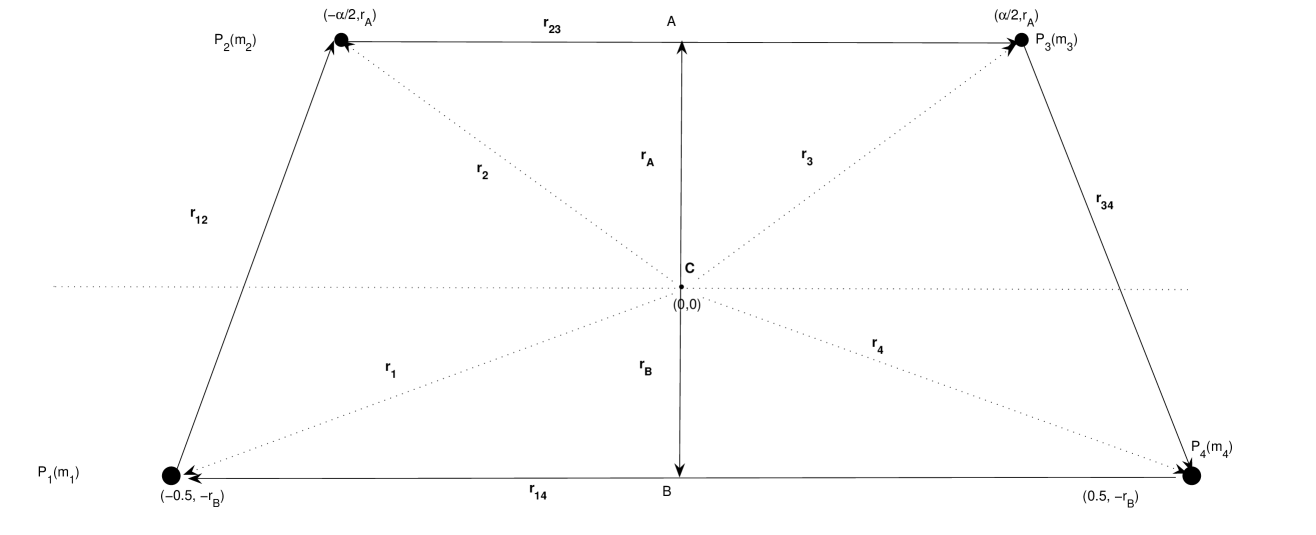
Figure 1: Trapezoidal Model

Theorem 2: Let $\mathbf{r}=(\vec{r}_{1},\vec{r}_{2},\vec{r}_{3},\vec{r}_{4})$ be a central configuration as defined in theorem 1. Then there exist a region $R={R_{f_{1}}}^{c}\cap{R_{f_{3}}}^{c})$ in the $\alpha\beta$-plane such that for any $\alpha,\beta\in R$ there exists positive masses $(m,M,m,M)$ making $\mathbf{r}$ a central configuration. The regions $R_{f_{1}}$ and $R_{f_{2}}$ are

$$R_{f_{1}}=\{(\alpha,\beta)|\alpha<g_{1}(\beta)\text{ and }0<\beta<1\}$$

$$R_{f_{3}}=\{(\alpha,\beta)|\alpha<g_{3}(\beta)\text{ and }0<\beta<1\}$$

where

$$g_{1}(\beta)=\frac{\sqrt{-2.\beta^{6}-1.5\beta^{4}+2\left(\beta^{2}+0.25\right)^{3/2}-0.375\beta^{2}-0.03125}}{\sqrt{1.5\beta^{4}+\frac{-0.75\beta^{2}-0.375}{\sqrt{\beta^{2}+0.25}}-0.09375}}.$$ (14)

$$g_{2}(\beta)=\sqrt{-\frac{\sqrt{\text{h1}^{2}-4\text{h0}\text{h2}}}{2\text{h2}}-\frac{\text{h1}}{2\text{h2}}}$$

Numerically, region $R$ is given by the colored part of figure (3b).

Before we prove theorem 1, we recall a lemma given by Roy and Steves [14].

Lemma 1:  Let $\mathbf{r=r}_{A}-\mathbf{r}_{B}$ (ref: figure 1) and then using the geometry of our proposed problem we arrive at the following relationships between $\mathbf{r}_{i},i=1,2,3,4,$ $\mathbf{r}$ and $\mathbf{r}_{41}.$

$$\mathbf{r}_{1} = -\frac{m}{M+m}\mathbf{r+}\frac{1}{2}\mathbf{r}_{41},$$

$$\mathbf{r}_{2} = \frac{M}{m+M}\mathbf{r+}\frac{\alpha}{2}\mathbf{r}_{41},$$

$$\mathbf{r}_{3} = \frac{M}{m+M}\mathbf{r-}\frac{\alpha}{2}\mathbf{r}_{41},$$

$$\mathbf{r}_{4} = -\frac{m}{M+m}\mathbf{r-}\frac{1}{2}\mathbf{r}_{41}.$$

2 The proof of theorem 1

Without loss of generality, it is assumed that the centre of mass of the system $\vec{c}=0$, $\vec{r}_{23}=-\alpha\vec{r}_{41}$, $r_{BA}=|\vec{r}_{A}-\vec{r}_{B}|=\beta r_{41}$. This gives us

$$\vec{r}_{B}=-\frac{m}{M}\vec{r}_{A}\text{ and }r_{A}=\frac{M\beta}{m+M}$$ (15)

Using these assumptions with equation (1) we obtain the following equations of motion.

$$\ddot{\mathbf{r}}_{1}=\frac{m\mathbf{r}_{12}}{\left(\left(0.5-\frac{\alpha}{2}\right)^{2}+\beta^{2}\right)^{3/2}}+\frac{m\mathbf{r}_{13}}{\left(\left(0.5+\frac{\alpha}{2}\right)^{2}+\beta^{2}\right)^{3/2}}+M\mathbf{r}_{14},$$ (16)

$$\ddot{\mathbf{r}}_{2}=\frac{M\mathbf{r}_{21}}{\left(\left(0.5-\frac{\alpha}{2}\right)^{2}+\beta^{2}\right)^{3/2}}+\frac{m\mathbf{r}_{23}}{\alpha^{3}}+\frac{M\mathbf{r}_{24}}{\left(\left(0.5+\frac{\alpha}{2}\right)^{2}+\beta^{2}\right)^{3/2}},$$ (17)

$$\ddot{\mathbf{r}}_{3}=\frac{M\mathbf{r}_{31}}{\left(\left(0.5+\frac{\alpha}{2}\right)^{2}+\beta^{2}\right)^{3/2}}+\frac{m\mathbf{r}_{32}}{\alpha^{3}}+\frac{M\mathbf{r}_{34}}{\left(\left(0.5-\frac{\alpha}{2}\right)^{2}+\beta^{2}\right)^{3/2}},$$ (18)

$$\ddot{\mathbf{r}}_{4}=\frac{m\mathbf{r}_{42}}{\left(\left(0.5+\frac{\alpha}{2}\right)^{2}+\beta^{2}\right)^{3/2}}\ +M\mathbf{r}_{41}+\frac{m\mathbf{r}_{43}}{\left(\left(0.5-\frac{\alpha}{2}\right)^{2}+\beta^{2}\right)^{3/2}}.$$ (19)

It is clear from lemma 1 that it is enough to study the equations for $\mathbf{r=}\frac{m+M}{2M}\left(\mathbf{r}_{2}+\mathbf{r}_{3}\right)$ and $\mathbf{r}_{41}$ as $\mathbf{r}_{i},i=1,2,3,4,$ are linear combination of $\mathbf{r}$ and $\mathbf{r}_{41}.$

$$\ddot{\mathbf{r}}_{41}=[-2M+\frac{m}{a}\left(\alpha-1\right)-\frac{m}{b}(\alpha+1)]\mathbf{r}_{41}.{\ \ \ \ \ \ \ \ \ \ \ \ }$$ (20)

$$\ddot{\mathbf{r}}_{3p2}=-[\frac{m+M}{a}+\frac{m+M}{b}]\left(\mathbf{r}_{2}+\mathbf{r}_{3}\right).{\ \ \ \ \ \ \ \ \ \ \ \ \ }$$ (21)

Using equation (3) in conjunction with equations (20) and (21) we obtain the following equations of central configurations for the trapezoidal four-body problem.

$$2M-\frac{m(\alpha-1)}{a}+\frac{m(\alpha+1)}{b}=\lambda,$$ (22)

$$\frac{m+M}{a}+\frac{m+M}{b}=\lambda.$$ (23)

It is a straightforward exercise to solve (22) and (23) to obtain (11) and (12). This completes the proof of theorem 1.

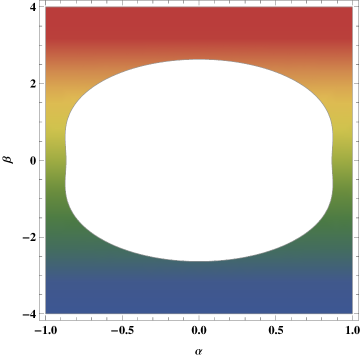
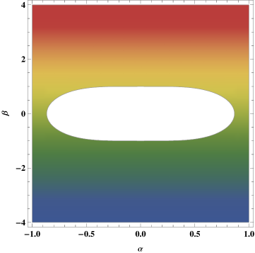
Figure 2:      a ) $R_{f_{1}}$ (white) where $f_{1}>0$.          b) $R_{f_{3}}$ (white) where $f_{3}>0$

Figure 3:      a) Region (colored), $R_{m}=(R_{f_{1}}\cap R_{f_{3}})\cup({R_{f_{1}}}^{c}\cap{R_{f_{3}}}^{c})$ b) The central configuration region ($R$) where both $m$ and $M$ are positive ( $R={R_{f_{1}}}^{c}\cap{R_{f_{3}}}^{c})$).

3 Proof of theorem 2

Let

$$f_{1}=a+b-2ab,f_{2}=a-b,f3=a+b-2ab+\alpha(a-b)$$

To find the region where the mass function $m$ is positive we need to find regions where

1. $f_{1}>0$,$f_{3}>0$,

2. $f_{1}<0$,$f_{3}<0$.

Similarly, for the mass function $M$ to be positive

1. $f_{2}>0$,$f_{3}>0$

2. $f_{2}<0$,$f_{3}<0$

To do a sign analysis of $f_{1}$, we will need to solve $f_{1}=0$. Its nearly impossible to solve $f_{1}>0$ . Therefore we write its polynomial approximation.

$$f_{1}aprox = \alpha^{2}\left(-1.5\beta^{4}+\frac{0.75\beta^{2}}{\sqrt{\beta^{2}+0.25}}+\frac{0.375}{\sqrt{\beta^{2}+0.25}}+0.09375\right)-2\beta^{6}-1.5\beta^{4}$$ (24)

$$+ 2\sqrt{\beta^{2}+0.25}\beta^{2}-0.375\beta^{2}+0.5\sqrt{\beta^{2}+0.25}-0.03125.$$

Now it is a straightforward exercise to show that $f_{1}>0$ in $R_{f_{1}}$.

$$R_{f_{1}}=\{(\alpha,\beta)|\alpha<g_{1}(\beta)\text{ and }0<\beta<1\}$$

where

$$g_{1}(\beta)=\frac{\sqrt{-2.\beta^{6}-1.5\beta^{4}+2\left(\beta^{2}+0.25\right)^{3/2}-0.375\beta^{2}-0.03125}}{\sqrt{1.5\beta^{4}+\frac{-0.75\beta^{2}-0.375}{\sqrt{\beta^{2}+0.25}}-0.09375}}.$$ (25)

Numerically, $R_{f_{1}}$ is given in figure (2a). The common denominator of $m$, and $M$ can be analyzed in a similar way.

$$f_{3}aprox = h_{2}\alpha^{4}+h_{1}\alpha^{2}+h_{0}$$ (26)

where

$$h_{0} = -2\beta^{6}-1.5\beta^{4}+2\left(\beta^{2}+0.25\right)^{3/2}-0.38\beta^{2}-0.03$$

$$h_{1} = -1.5\beta^{4}-\frac{0.75\beta^{2}}{\sqrt{\beta^{2}+0.25}}+0.1$$

$$h_{2} = (-0.375\beta^{6}-0.09\beta^{4}+\left(-0.19\sqrt{\beta^{2}+0.25}-0.023\right)\beta^{2}-0.031\sqrt{\beta^{2}+0.25}$$ (27)

$$+ \frac{0.047\beta^{4}}{\sqrt{\beta^{2}+0.25}}-0.006)\frac{1}{\left(1.\beta^{2}+0.25\right)^{2}}$$

Using approximate techniques with help from symbolic computation in Mathematica it can be shown that $f_{3}$ attains positive values in the following region.

$$R_{f_{3}}=\{(\alpha,\beta)|\alpha<g_{3}(\beta)\text{ and }0<\beta<1\}$$

where

$$g_{2}(\beta)=\sqrt{-\frac{\sqrt{\text{h1}^{2}-4\text{h0}\text{h2}}}{2\text{h2}}-\frac{\text{h1}}{2\text{h2}}}$$

Numerically, $R_{f_{3}}$ is given in figure (2b).

Therefore the central configuration region where $m>0$ is given by

$$R_{m}=(R_{f_{1}}\cap R_{f_{3}})\cup({R_{f_{1}}}^{c}\cap{R_{f_{3}}}^{c})$$

Numerically, $R_{m}$ is given in figure (3). As $f_{2}<0$ for all values of $\alpha$ and $\beta$ therefore $M>0$ in the region where $f_{3}<0$. This region is numerically represented by the colored part of figure (2b) and analytically by the compliment of ${R_{f_{3}}}.$ Hence the central configuration region ($R$) where both $m$ and $M$ are positive is given by $R=({R_{f_{1}}}^{c}\cap{R_{f_{3}}}^{c})$. Numerically this region is given in figure (3b).

4 Conclusions

In this paper we model non-collinear trapezoidal four-body problem where the masses are placed at the vertices of an isosceles trapezoid. Expressions for $m$ and $M$ are formed as functions of $\alpha$, and $\beta$ which gives central configurations in the trapezoidal four-body problems. We show that in the $\alpha\beta$-plane, $m$ is positive when $(\alpha,\beta)\in R_{m}$. Similarly $M$ is positive when $(\alpha,\beta)\in R_{f_{3}}^{c}$. We have identified regions in the $\alpha\beta$-plane where no central configurations are possible. A central configuration region $R=({R_{f_{1}}}^{c}\cap{R_{f_{3}}}^{c})$ for the isosceles trapezoidal 4-body problem is identified in the $\alpha\beta-$ plane where $m$ and $M$ are both positive. No central configurations are possible outside this region unless we allow one of the masses to become negative.

Acknowledgement: The author thanks the Deanship of research at the University of Hail, Saudi Arabia for funding this work under grant number SM14014.

References

[1] A. Albouy and J. Llibre.
Spatial central configurations for the 1+4 body problem.
Contemporary Mathematics, 292:1–16, 2002.
[2]K. R. Meyer. ”Bifurcation of a central configuration.” Celestial Mechanics and Dynamical Astronomy 40.3 (1987): 273-282.
[3] M. Hampton and R. Moeckel, ”Finiteness of relative equilibria of the four-body problem. Inventiones mathematicae”, 163(2), 289-312, 2006.
[4]M. Kowalczyk. ”Bifurcations of critical orbits of invariant potentials with applications to bifurcations of central configurations of the N-body problem.” arXiv preprint arXiv:1501.07449, 2015.
[5]M. Shoaib, A. Sivasankaran and A.R. Kashif ”Central configurations in the collinear five-body problem”, Turkish Journal of Mathematics, 38 (3), 576-585, 2014.
[6]M. Shoaib, A. Sivasankaran and Y. Abel Aziz , ”Central Configurations in a symmetric five-body problem”, Chaotic Modeling and Simulation, 3 (3), 431-439, 2014.
[7]A. Sivasankaran and M. Shoaib , ”An efficient computational approach for global regularization schemes”, Chaotic Modeling and Simulation, 3 (3), 441-450, 2014.
[8] M. Shoaib, I. Faye, and A. Sivasankaran, A. Some special solutions of the rhomboidal five-body problem. In INTERNATIONAL CONFERENCE ON FUNDAMENTAL AND APPLIED SCIENCES 2012:(ICFAS2012) (Vol. 1482, No. 1, pp. 496-501). AIP Publishing, 2012.
[9] M. Shoaib, ”Regions of Central Configurations in a symmetric 4+ 1-Body Problem”, Advances in Astronomy, 2015, 1-7, 2015.
[10]M. Shoaib and I. Faye , ”Collinear equilibrium solutions of four-body problem”, Journal of Astrophysics and Astronomy, 32, 411-423, 2011.
[11]M. Shoaib, B.A. Steves and A. Szell, ”Stability analysis of quintuple stellar and planetary systems using a symmetric five body model”, New Astronomy 13, 639-645, 2008
[12]M. Sekiguchi. ”Bifurcation of central configuration in the 2n+ 1 body problem.” Celestial Mechanics and Dynamical Astronomy 90, no. 3-4 355-360, 2004.
[13] D. Rusu and M. Santoprete, ”Bifurcations of Central Configurations in the Four-Body Problem with some equal masses”. arXiv preprint arXiv:1412.6443, 2014
[14] A.E. Roy and B.A. Steves, ”Some special restricted four-body problemsII. From Caledonia to Copenhagen”. Planetary and space science, 46(11), 1475-1486, 1998.