The SEGUE K Giant Survey. III. Quantifying Galactic Halo Substructure

Abstract

We statistically quantify the amount of substructure in the Milky Way stellar halo using a sample of 4568 halo K giant stars at Galactocentric distances ranging over 5-125 kpc. These stars have been selected photometrically and confirmed spectroscopically as K giants from the Sloan Digital Sky Survey’s SEGUE project. Using a position-velocity clustering estimator (the 4distance) and a model of a smooth stellar halo, we quantify the amount of substructure in the halo, divided by distance and metallicity. Overall, we find that the halo as a whole is highly structured. We also confirm earlier work using BHB stars which showed that there is an increasing amount of substructure with increasing Galactocentric radius, and additionally find that the amount of substructure in the halo increases with increasing metallicity. Comparing to resampled BHB stars, we find that K giants and BHBs have similar amounts of substructure over equivalent ranges of Galactocentric radius. Using a friends-of-friends algorithm to identify members of individual groups, we find that a large fraction ($\sim$33%) of grouped stars are associated with Sgr, and identify stars belonging to other halo star streams: the Orphan Stream, the Cetus Polar Stream, and others, including previously unknown substructures. A large fraction of sample K giants (more than 50%) are not grouped into any substructure. We find also that the Sgr stream strongly dominates groups in the outer halo for all except the most metal-poor stars, and suggest that this is the source of the increase of substructure with Galactocentric radius and metallicity.

1 Introduction

Current cosmological models predict that structure forms through hierarchical processes. For galaxies, the hierarchical assembly model implies that satellite galaxies will be tidally disrupted, leaving stellar debris (Bullock & Johnston, 2005; Cooper et al., 2010). Large–scale surveys like the Sloan Digital Sky Survey (SDSS; York et al., 2000) and the Two Micron All Sky Survey (2MASS; Skrutskie et al., 2006) have the capability to find these substructures around the Milky Way. Kinematic and chemical information derived from these observations then allow for more detailed analysis of the history of the buildup of the Galaxy.

The search for stellar substructure in and around the Milky Way has been remarkably successful (cf. Belokurov et al., 2006). In addition to the the Sagittarius dwarf spheroidal galaxy (Sgr; Ibata et al., 1994), and its associated tidal stream (Mateo et al., 1996; Majewski et al., 2003), about a dozen presumably distinct streams or overdensities have been discovered photometrically (Duffau et al., 2006; Grillmair & Dionatos, 2006; Belokurov et al., 2007; Newberg et al., 2007, 2009, 2010; Grillmair, 2014). These streams have a variety of morphologies, ranging from thin, kinematically cold streams to ‘clouds’, and may comprise the majority of all halo stars beyond $\sim 15$ kpc (Bell et al., 2008).

By collecting the spatial and kinematic properties of Galactic stars, a statistical analysis of substructure in the Galactic stellar halo becomes possible. Precedent for this kind of analysis is widespread. Maps of stellar density are a classical method of finding substructure. Substructure regions will appear to be more dense on the sky than a smooth background of stars. Large–scale photometric surveys are well suited to this method. For example, Belokurov et al. (2006) used a simple color cut on a sample of SDSS stars which highlighted a number of structures in the Milky Way halo, including the Sgr tidal streams, the Orphan Stream, and Monoceros ring. With multi-color photometric data, this analysis can also be extended to population information. Bell et al. (2008) quantified the variation in star counts in the color region dominated by halo main sequence stars, and Deason et al. (2011) made a similar calculation using blue horizontal branch (BHB hereafter) stars, and found a smaller variation in star counts at the same distances. This result is intriguing because, while all stars start their lives on the main sequence, only those with a certain range of age and metallicity evolve to become BHB stars, which are typical of old, metal poor populations. Thus the smaller amount of substructure seen in BHB stars may be due to a population difference rather than simply indicating a smoother halo than previously thought, as claimed by Deason et al. (2011).

Use of kinematic data enhances a metric’s ability to distinguish substructure from its surrounding smooth distribution. Gorski et al. (1989)’s method is similar to the classic two-point correlation function, in that it uses a random smooth distribution for significance testing, but the metric instead finds the probability that two objects separated by a given distance will have the same velocity, rather than the number of pairs at a given separation in distance. This metric has been largely used in cosmological clustering studies, but could be easily adapted to stellar kinematic data. Schlaufman et al. (2009) identify substructure by exploring the radial velocity distributions of metal-poor main-sequence turnoff stars on individual SDSS plug-plates (hereafter, plates). This tracer limits them to the inner halo: distances of 17.5 kpc and less. This method requires a fairly dense sample to be effective, since it makes use of velocity distributions. Schlaufman et al. (2009) used nearby SDSS dwarfs in their analysis, but were still able to identify ten stellar structures in the nearby halo and make predictions about the overall membership of stars in substructure, finding that $1/3$ of the volume of the local halo contains velocity substructure.

The logical extension of this progression is to use all six dimensions of phase space $(x,y,z,v_{x},v_{y},v_{z})$ to identify substructure. Given the very accurate observations that are required to measure all six of these dimensions, and the current capabilities of large–scale ground based surveys, only four of these dimensions are readily available. Starkenburg et al. (2009) used a sample of 101 K giants from the Spaghetti survey (Morrison et al., 2000), with distances up to $\sim$100 kpc and line-of-sight velocities to determine the overall amount of substructure in the Milky Way stellar halo, finding that it is indeed highly structured, but less so than simulated halos derived from Harding et al. (2001). This difference is due to the sparse spatial sampling of the Spaghetti survey being unable to resolve narrow streams in the halo, an issue which Starkenburg et al. (2009) suggest could be alleviated by a much larger survey. Additionally, the authors were able to identify a number of stars associated with the Sagittarius stream and Virgo overdensity using a friends-of-friends group finding algorithm.

Analysis of a much larger sample of SDSS BHB stars with $5~{}\textrm{kpc}<R_{gc}<60~{}\textrm{kpc}$ by Xue et al. (2011) (hereafter X11) demonstrated with very high significance that position–velocity substructure exists throughout the Milky Way halo. With this sample, X11 showed that the outer halo was more structured than the inner halo, and that these observations were consistent with, but less prominent than, levels of substructure in mock catalogs derived from the Bullock & Johnston (2005) models. X11 attributed the difference with the models to the strong representation of BHB stars in older stellar populations, showing that the older model particles also exhibited less substructure. Further, Cooper et al. (2011) used ($x,y,z$) and line-of-sight velocity to quantify substructure in mock catalogs from the Aquarius stellar halo models (Springel et al., 2008; Cooper et al., 2010), comparing this with a smaller sample of SDSS BHB stars from Xue et al. (2008). Interestingly, they find that the clustering signal for stars 20-60 kpc from the Galactic center is consistent with the range of clustering in the Aquarius models, but for inner halo stars the signal is lower than all of the model halos. They suggest that this lack of substructure may be due to a smooth component of the inner halo.

Studying the amount of halo substructure in red giants is preferable to solely using BHB stars, as all intermediate-age and old stars, regardless of metallicity, turn into red giants. We note that K giants are drawn from a larger range of age and metallicity than BHB stars, and so comparisons between substructure in the two groups could be very helpful. In this study, we present a considerably larger set of red giants than in Starkenburg et al. (2009) to overcome the problems of statistical sampling and provide a more robust comparison with simulations. We use a statistical method called the 4distance (Starkenburg et al., 2009, described fully in Section 3) to quantify the substructure in the largest and most spatially diverse spectroscopic K giant sample to date. In Section 2, we describe our sample and the methods used to construct it. In Section 3 we also discuss other methods used in this paper, including normalization techniques and the friends-of-friends group finding algorithm. In Sections 4 and 5, we present our results.

2 The sample

The Sloan Extension for Galactic Understanding and Exploration (SEGUE) obtained nearly 350,000 spectra of 21 different target types in its four years of observations (Yanny et al., 2009a, C. Rockosi et al. in preparation, York et al., 2000; Gunn et al., 2006; Eisenstein et al., 2011; Smee et al., 2013). The definition, calibration and verification of our K giant sample is described in detail in H. Morrison et al. (in preparation), and the Bayesian distance estimation technique we employ is described in Xue et al. (2014). Here we provide an overview only.

SEGUE used a pencil-beam sampling of the sky, which can be seen in Figure 3. The SDSS $ugriz$ system (Fukugita et al., 1996) was not designed for studying stars, so targeting possible giants was not as easy as it would have been with, for example, specially designed filters such as the DDO 51 filter (Geisler, 1984). Three target types aimed to identify K giants; all three used regions of the $u-g$/$g-r$ color-color diagram. The first target type ($l$-color K giants), designed to identify metal-poor giants of the halo, used the metallicity sensitivity of the $u-g$ color at the bluer end of the K giant region to identify halo giants. However, this method does not work for the redder stars: as discussed in Yanny et al. (2009a) and illustrated in their Figure 10, the giant sequence crosses the foreground dwarf locus around $(g-r)_{0}$=0.8, and appears above the foreground locus for even redder $g-r$. SEGUE used two target types to identify K giants here: the red K giant and proper motion K giant categories.

We identified our K giants by first finding all the stars in SDSS data release 9 (DR9; Ahn et al., 2012) with spectra which also satisfied the $ugr$ and other requirements for target selection of the three types discussed above. We limited our consideration to stars with $E(B-V)$ from Schlegel et al. (1998) less than 0.25 mag. We then used the SEGUE spectra to measure each star’s luminosity by first taking a log $g$ value from the SEGUE Stellar Parameters Pipeline (SSPP; Lee et al., 2008) as an initial cut (log $g$ $<$ 3.5), then using the Mg index, mirroring the method described in Morrison et al. (2003), to identify giants. As well as the three target selection categories, there were spectroscopically confirmed giants which do not satisfy the selection criteria of any of the three target types described above: we refer to them as serendipitous K giants.

Our overall aim in this paper is to quantify the amount of substructure in the Milky Way’s stellar halo, and thus we need to exclude (thick) disk stars from our sample. While SEGUE’s giant classification was aimed at identifying giants in the halo, there are fields (particularly at low latitude) where thick disk giants dominate.

We have chosen not to use a model of the structure of the disk/thick disk in our work, since the structure of the thick disk away from the solar cylinder, in particular, is still an active area of research. Instead, we used both spatial cuts and also a kinematic cut, excluding stars which satisfy all of the following criteria: [Fe/H]$>-1.0$,$|z|<10$ kpc, the distance from the Galactic center in the plane $R<20$ kpc, and the star is located inside the region of the longitude-velocity plot shown in blue in Figure 2.

We chose a metallicity cut as disk stars are on average much more metal-rich than halo stars. Since there are a few halo stars with [Fe/H] greater than –1.0 even in the solar neighborhood (see, for example Carney et al., 1996), and there may be some thick disk stars with [Fe/H] less than –1.0 (the metal-weak thick disk stars discussed below), we used a cut of [Fe/H]  $>-1.0$ as a good compromise.

Making a cut on distance from the center of the Galaxy also required a compromise. Many Sgr orbit models (e.g. Law & Majewski, 2010, ; LM10 hereafter) show perigalactic distances around 15-20 kpc. By contrast, although the position of the edge of the Galactic disk is not well constrained, it is likely to be between 15 and 20 kpc from the Galactic center (Reylé et al., 2009; Carraro et al., 2010). We have chosen 20 kpc as the best distance limit here. Our choice of a cut in $z$ height ($|z|<10$ kpc) might seem high for a thick disk scale height of order 1 kpc (Majewski, 1993; Jurić et al., 2008). However, given the expectation that the numbers of a stellar population in a pencil-beam survey peak at 2-3 times its scale height due to the volume element growing with distance, we have chosen a conservative cut in order to exclude as many thick disk stars as possible.

Our last criterion employs a longitude-velocity plot (often used in studies of gas dynamics because a distance estimate is not readily available) in order to require that the star has kinematics consistent with the disk/thick disk. Figure 1 both highlights the kinematics of our giant sample to show how the disk/thick disk appears in these plots, and also shows how bright streams such as those from the disruption of the Sgr dwarf galaxy will appear. The Figure shows the radial velocity (corrected to account for the LSR velocity around the Galactic center) versus Galactic longitude for our enlarged K giant sample ($\sim$15,000 stars). Here we have included another 10,046 stars not presented in the X14 sample because they are bluer than the intersection of the horizontal and giant branches and so have two possible distances. We know that these stars are giants, but do not know their distances. Because we do not need the distance of a star to place it on the longitude-velocity plot, we can increase our sample size by a factor of three here, and see the kinematic patterns more clearly. The top panel shows the entire sample. There are two patterns of clumping in the longitude-velocity plane: one which is most visible for $l<180$, showing positive velocities which peak near 200 km s^-1, and the other which shows negative velocities and is visible for almost the entire range of longitude.

Figure 1: The signature of the disk and of the Sgr dSph stream in a plot of Galactic longitude $l$ against the line of sight velocity of the star, corrected for the projection of the LSR velocity along the line-of-sight. The top three panels are drawn from our extended K giant sample of 15,081 giants, while the bottom panel comes from the smaller sample of K giants with distances from X14. The top panel shows the entire extended K giant sample. The next lower panel shows stars at low latitude ($|b|<35^{\circ}$) with high metallicity ([Fe/H]$>-0.5$). The signature of disk rotation is clear here (note that we lack stars at low latitude and longitude greater than 240 deg. because the SDSS telescope is in the North). The third panel shows stars with the same low latitude cut, but [Fe/H]$<-1.0$, and in contrast, displays a symmetry between negative and positive velocities typical of the halo. The last panel includes giants with distances greater than 20 kpc from the Galactic center. The signature of the Sgr dSph stream is clearly seen here.

The second panel shows the $l-v$ distribution of more metal-rich stars ([Fe/H]$>-0.5$) at low latitude ($|b|<35^{\circ}$). One would expect these criteria to isolate stars from the Galaxy’s disk and thick disk. Since Galactic rotation is defined to be positive in the direction $l=90^{\circ}$ (Binney & Merrifield, 1998), we see that the chosen stars have the correct sign of velocity for disk objects. The range of $v_{gsr}$ seen for disk stars is a function of both their position along the line-of-sight and of their population’s velocity dispersion. Since $V_{\phi}$ is the only component of the velocity of a disk/thick disk star with non-zero mean, a star whose position places the direction of $V_{\phi}$ close to the line-of-sight will show a significant velocity in the direction of rotation of the Galaxy’s disk. Conversely, stars at the anticenter will have velocity close to zero because $V_{\phi}$ is orthogonal to the line-of-sight there, as can be seen in this panel. As a star’s latitude increases, the component of $V_{\phi}$ along the line of sight will also decrease because of projection. The velocity dispersion of the population along the line-of-sight will then ‘jiggle’ the star’s position away from its geometric expectation.

The third panel shows stars from the same latitude range ($b<35^{\circ}$), chosen to have [Fe/H] less than –1.0. Here we see a completely different velocity distribution, which is basically symmetric around zero velocity, except for some substructure likely to be stellar streams. This symmetry in velocity suggests that the stars belong to the Galactic halo, which has a near-zero mean velocity (eg Zinn, 1985; Fermani & Schönrich, 2013). We also see little contribution from the metal-weak thick disk (Norris et al., 1985; Morrison et al., 1990; Carollo et al., 2010) in our sample.

Lastly, the bottom panel shows only giants with distances available in X14, which are chosen to have $R_{gc}>20$ kpc. Since the edge of the Galaxy’s disk is at approximately this distance, we would expect this criterion to exclude most disk stars and all stars from the inner halo. The feature which we can see stretching across values of longitude from 60 to 360 is caused by the various wraps of the Sgr dSph, and will be discussed in more detail in Section 3.4. Since the pericenter of the orbit of the Sgr dwarf is at $R_{gc}\sim$ 17 kpc (Law & Majewski, 2010) and the current position, close to pericenter, is in the Southern Hemisphere, and thus not accessible to SEGUE, we should see almost all Sgr members in our sample in this panel.

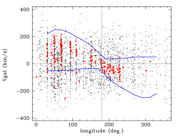
Figure 2: Galactic longitude vs radial velocity, corrected for the motion of the LSR projected on the line-of-sight for all stars with $R<20$ kpc and $|z|<10$ kpc. Stars with [Fe/H]$>-0.8$ are shown in red. The blue line outlines the region we have chosen to contain likely disk stars.

Figure 2 illustrates the velocity cut we apply to remove disk stars from our sample. We show all stars with $R<20$ kpc and $|z|<10$ kpc, highlighting those with [Fe/H]  greater than –0.8. It can be seen that almost all of the red symbols are inside the blue lines which indicate the velocity cut.

In summary, we exclude stars as possible disk or thick disk members if they satisfy two spatial criteria (in R and z) and a kinematical criterion. When these cuts are applied, we end up with 4568 stars in our halo sample.

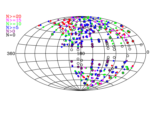
Figure 3: The SEGUE plate footprint in the Galactic coordinate system. Each point represents a plate center. The color represents the number of spectroscopically confirmed K giants in our sample on each plate (between 0 and 25), illustrating that some regions on the sky are more dense in K giants than others.

Spatial substructure is visible in the number of giants found per field. While the actual giant density needs corrections for our observing strategy in a way similar to that of Bovy et al. (2012) or Schlesinger et al. (2012), Figure 3 demonstrates that even the uncorrected numbers vary from field to field and between hemispheres in a manner suggestive of spatial overdensities. We note, however, that the fields with low latitude ($|b|<20^{\circ}$) shown as having no giants were excluded from our giant sample because of their high reddening or because of our disk star exclusion algorithm.

We adopt the SSPP [Fe/H] measurement without applying any further corrections, as H. Morrison et al. (in preparation) have shown that these [Fe/H] values closely correspond with literature values for our calibration sample of star clusters and stars with high-resolution spectroscopy. Typical errors in [Fe/H] are 0.15 to 0.20 dex.

Figure 4: [Fe/H] distribution for the spectroscopically confirmed K giant sample with 4568 giants. The vertical dashed and dot-dash lines show the ranges of [Fe/H] we use to create metallicity subsamples below. The dot-dash line represents the median value ([Fe/H] $\approx-1.5$).

The metallicity distribution of our entire sample of 4568 giants is shown in Figure 4. However, we caution the reader against drawing any conclusions about the metallicity histogram of the halo from this diagram, as each target type produces a different metallicity distribution (with the red K giant distribution having a higher mean metallicity, for example), which are not corrected for here. The metallicity distribution of the halo will be the subject of a future paper (Z. Ma et al., in preparation). However, we note that there are a significant number of stars in our halo sample with [Fe/H] greater than –1.0. Although traditionally halo stars have been thought to be metal-poor, local halo samples from earlier work such as that discussed in Carney et al. (1996) have so much contamination from the thick disk that the actual number of halo stars with metallicities greater than –1.0 has not been well constrained.

Figure 5: Histogram of Galactocentric radius for the 4568 member K giant sample, with distances from Xue et al. (2014).

We used distances for the SEGUE K giants given by Xue et al. (2014), calculated using a Bayesian technique, which relies on fiducial giant branch sequences for different metallicities and, importantly, makes corrections for the fact that stars near the tip of the giant branch are much rarer than stars lower down the giant branch. Xue et al. (2014) show that ignoring this will lead to a bias of 10% in distance modulus on average, reaching 20% in some cases. Figure 5 shows the distribution of distances in our sample: the dataset has significant numbers of K giants at distances of more than 50 kpc, a great improvement on previous halo samples.

3 The 4distance

There have been many approaches to measuring substructure: one of the simplest being simply to count the number of halo turnoff stars. This technique highlights spatial overdensities in the halo, which are particularly apparent in the early stages of a stream’s disruption (Bullock & Johnston, 2005). Our Figure 3 shows suggestions of such spatial overdensities, but would require a proper correction for our complex SEGUE observational strategy to be compared with data such as the ‘Field of Streams’. Another simple approach is to study the velocity distribution in different fields of a pencil-beam survey, as modeled by Harding et al. (2001) and implemented by Schlaufman et al. (2009): deviations from a smooth shape in halo fields are likely to be caused by disrupted streams, and this has the advantage of retaining a signal for later stages of disruption. In Figure 6 we show some typical velocity histograms from giants in SEGUE fields. It can be seen that few of these histograms have smooth or near-Gaussian velocity fields, suggesting a large degree of substructure in our halo sample.

Figure 6: Examples of velocity distributions (showing $v_{gsr}$, with the projection of the LSR and solar velocity on the line-of-sight removed) for K giants on individual plates. The label in each quadrant shows the plate number and $(l,b)$ coordinates.

The method that we have chosen to study substructure combines several different dimensions of data: position on the sky, distance, and velocity. As in X11, we use the 4distance method of Starkenburg et al. (2009, S09 hereafter). This metric takes advantage of SEGUE’s capability to measure several dimensions in phase space, specifically latitude, longitude, line-of-sight radial velocity, and distance ($l,b,v_{los},d_{sun}$). The 4distance calculates the separation of two stars in each of these four quantities, applies a weighting factor dependent on the measurement range and error, and then produces a dimensionless distance in phase space,

$$\delta_{4d}^{2}=w_{\phi}\phi_{ij}^{2}+w_{v}(v_{i}-v_{j})^{2}+w_{d}(d_{i}-d_{j})^{2},$$ (1)

where the angular separation $\phi_{ij}$ is defined by:

$$\cos\phi_{ij}=\cos b_{i}\cos b_{j}\cos(l_{i}-l_{j})+\sin b_{i}\sin b_{j}.$$ (2)

The three weighting factors ($w_{\phi},w_{d},w_{v}$) in the 4distance have a two-fold function: to scale the result to physical quantities and to take into account the measurement errors of the data in the metric itself. These weights are defined as

$$w_{\phi}=\frac{1}{\pi^{2}},$$ (3)

$$w_{d}=\frac{1}{130^{2}}\frac{(\frac{d_{err}(i)}{d(i)})^{2}+(\frac{d_{err}(j)}{d(j)})^{2}}{2<\frac{d_{err}}{d}>^{2}},$$ (4)

and

$$w_{v}=\frac{1}{500^{2}}\frac{v_{err}^{2}(i)+v_{err}^{2}(j)}{2<v_{err}>^{2}}.$$ (5)

Since the error in angular position is negligible, it is not included here. However, velocity and distance both often have a significant error component. In our case, distance error scales with distance, but velocity error does not scale with velocity. This is reflected in the weighting factors. The choice of the constant in the weighting factor is determined by the range of the observed quantities and represents the maximum separation between two stars in the 4distance metric.

Table 1: Maximum physical component size for a selected 4distance ($4\delta=0.03$)

Component	Size
$\phi$ $(l,b)$	$5.4^{\circ}$
distance (heliocentric)	6 kpc
velocity (Galactocentric standard of rest)	15 km s-1

Table 1 shows some examples of physical sizes corresponding to a 4distance of 0.03. For example, if the 4distance was calculated for two stars with identical values of l, b and distance, then a difference of 15 km s^-1 in velocity would produce a 4distance of 0.03. For stars on the same SEGUE plate, the range in 4distance can be quite large for plates with large numbers of ($>20$) stars. An extreme example is plate 3245, which has 36 stars and has a minimum 4distance of 0.006, median 4distance of 0.185, and maximum 4distance of 1.084. For stars separated by a plate diameter (2.98 deg), the minimum 4distance (equal velocity and distance) is 0.016.

We define a pair of stars as being two stars separated by no more than a certain 4distance. We can, in effect, derive a two-point correlation function in a sample by comparing the number of pairs we observe to the number we would expect from a smooth distribution. The exact value we measure is the ratio of the cumulative number of pairs in the data with $\delta_{4d}$ less than a certain value to the number of pairs in a “smooth” sample (we describe the characteristics of a smooth sample in Section 3.1), which we will refer to as the 4distance ratio. As $\delta_{4d}$ (or the 4distance bin) increases, we expect the 4distance ratio to approach one as the cumulative number of pairs in the data and smooth sample become equal, meaning that at larger separations, there are no additional pairs being added to the cumulative sum. Error bars on our measurements are simply due to Poisson statistics, modeled using a Monte Carlo approach.

When small values $(\delta_{4d}<0.10)$ of the 4distance have a relatively large signal, we can infer the existence of streams and other cold substructure in the sample. The 4distance is a robust measurement of the amount of substructure in a population, but is not always an ideal indicator of the presence of streams. The spectrographic plate design of the SDSS forces objects on the same plate to be observed at relatively small angular separations, which causes the bulk of the contribution to the 4distance between two stars on the same plate to be from velocity and distance. The number of pairs will also vary as a function of distance. Whether through a magnitude limit or the halo density distribution function, the number density of stars decreases with increasing distance. This relationship causes a distant star to be less likely to be paired with another, but emphasizes the significance of finding pairs at large distances.

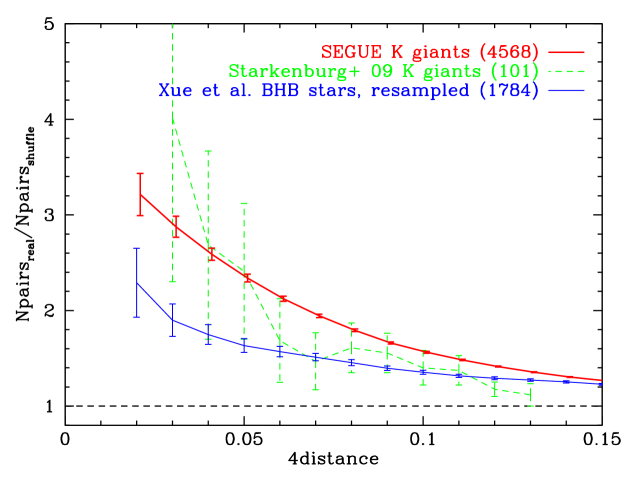
Figure 7: 4distance measurements for our K giants (red), those of Starkenburg et al. (2009) (green dashed), and a resampled set of BHB stars from X11 (blue) using the shuffle method of normalization used by Starkenburg et al. (2009)

3.1 Normalization with a Smooth Halo Model

3.1.1 Motivation

In order to normalize the global indicator of substructure (the $4\delta$ ratio) we need to find the number of 4distance pairs we would expect to see in a smooth halo. S09, X11, and Cooper et al. (2011) solved the problem of normalization by randomly shuffling their data. By holding $(l,b)$ constant and independently shuffling $v_{gsr}$ and $d_{sun}$, it was possible to approximate a smooth halo while respecting a survey footprint. We compared the pair counting results for our K giant sample to a shuffle normalization; the results are shown in Figure 7. The measurement for our order of magnitude larger sample is consistent with the S09 measurement. We see that, for a given value of 4distance, the K giants have between 1.5 and 2 times more pairs than the BHB stars that have been resampled to select those only inside the SEGUE footprint: they show signficantly more substructure. However, their radial distribution is different, with the K giants stretching to twice the distance of the BHB stars because of their larger luminosity. X11 have shown that the amount of substructure in their BHB sample increases with distance from the galactic center, and we will show that the K giants have a similar property in Section 4.1. We will further investigate the K giant/BHB differences in Section 4.3.

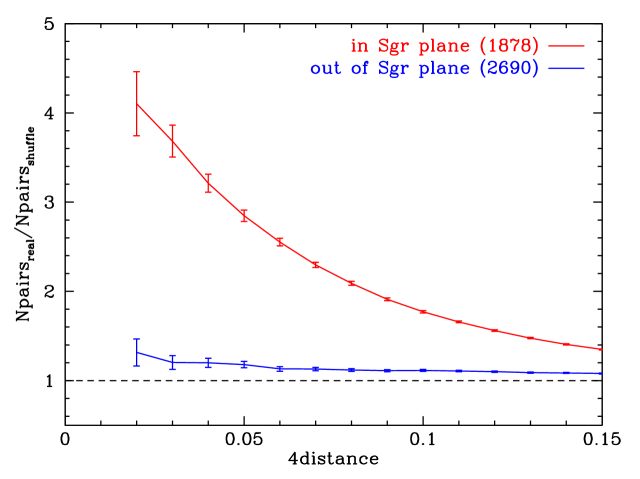
Figure 8: 4distance measurements for K giants in the Sgr plane ($|B|<12$; magenta) and out of the Sgr plane ($B>|12|$; cyan) using the shuffle method of normalization used by Starkenburg et al. (2009). As expected, the stars in the Sgr plane show a much higher substructure signal than stars out of the Sgr plane.

To show one way the 4distance metric can be used to quantify substructure in the halo, we have divided the K giant sample based on its position in the Sgr coordinate system ($\Lambda$, $B$) described by Majewski et al. (2003). Stars with $|B|<12$ are classified as being in the Sgr plane, while all other stars are outside of the plane. We show the results of 4distance pair counting for these two subsamples in Figure 8. We obtain the expected result, which is that stars in the Sgr plane show a significantly larger amount of substructure than stars out of the Sgr plane.

However, we note that shuffling normalization method does not account for all aspects of spatial substructure since it leaves the number of stars at each ($l,b$) constant. We know that spatial substructure is quite obvious in large samples (see Belokurov et al. (2006)), so we wish to include spatial position in the metric. SEGUE’s pencil-beam spectroscopic footprint has an uneven spatial sampling, so to understand the effect of spatial distribution on the measurement of the 4distance ratio we must “observe” a smooth halo model. Further, spatially concentrated structures are more likely to be identified with the 4distance metric, but will be unaccounted for in the pair ratio when using a shuffle normalization. Thus we have chosen to use a smooth halo model for our normalization, instead of following S09 and shuffling velocity and distance in the survey footprint. We will see below that adding the additional spatial information by using a smooth halo for normalization increases the substructure signal by a factor of $\sim$ 1.4 for our sample.

3.1.2 Assumptions

Our choice of a smooth halo model for normalization, while adding sensitivity to substructure, requires assumptions about the properties of a smooth halo, the first of which is the density distribution of stars. We use a power-law density distribution, $\rho\propto r^{-3.5}$ (see Zinn, 1985; Preston et al., 1991; Vivas & Zinn, 2006). It is important to use a reasonable estimate for stellar density because the number of observed pairs depends on the density itself (more dense regions will have more pairs), and we do not want to over-count pairs in the smooth halo, as this would decrease the overall substructure signal. We will use a $\rho\propto r^{-3.0}$ halo model in Section 3.3 to test this effect. Next, we assume a functional form for the velocity distribution of the smooth halo. This choice is less critical than the choice of the density distribution because the velocity component of the 4distance is the one with the smallest bin size compared to the overall range. We choose the velocity ellipsoid from Morrison et al. (1990), $(\sigma_{x},\sigma_{y},\sigma_{z})=(133,98,94)$ km s^-1 in an attempt to realistically model the halo, but make comparisons to a uniform velocity ellipsoid in Section 3.3.

Our next set of assumptions concern the observational constraints from our survey. The first two relate to the distance distribution of our sample, but the most important of these is the luminosity function. K giants in SEGUE are a subset of target types, and different target types have different distributions in absolute magnitude. This matters because it affects the K giant detection limits in the halo: some target types are redder stars, which can be intrinsically more luminous. Therefore we create an absolute magnitude distribution for the stars to which we attempt to match the absolute magnitude distribution of the model points. We also need to take into account the apparent magnitude and $R_{gc}$ distributions. The reason for this is to be sure that our model points have a similar, but not explicitly identical, distribution to our data. The apparent magnitude distribution is also not flat, so we treat that the same way as the luminosity function, but also ensure that the $R_{gc}$ distribution is similar to that of the data. The simplest of the observational constraints is the SEGUE plate footprint. Here, we only require a model point to be within 1.49 degrees of a SEGUE plate center. Finally, we require the overall number of points to be the same as observed, and the number of each target type the same as observed.

3.1.3 Technique

Because the four target categories have different apparent magnitude and luminosity distributions, we generate points for our smooth halo model for each target category separately. Since the smooth halo needs the same number of points as the actual dataset we are testing for substructure, we count the number of stars from each category, and produce a smooth model with the same number of stars. We produce a random sample with density distribution $\rho\propto r^{-3.5}$ within the observed range of $R_{gc}$ for each target category. We then generate an absolute magnitude (uniformly in the range [$1,-3$]), calculate the apparent magnitude directly from the random distance and absolute magnitude, then randomly select model stars based on the actual distributions of apparent and absolute magnitude for that target category, and check that the point falls within the correct $R_{gc}$ bin for that combination of ($l,b$) position, apparent magnitude, and absolute magnitude. This procedure has the effect of allowing us to generate an $R_{gc}$ distribution similar to that of the data, but drawn from a smooth underlying population. Also, we only keep points which are within the SEGUE footprint on the sky. Each point is then assigned velocities from the Morrison et al. (1990) velocity ellipsoid with $(\sigma_{x},\sigma_{y},\sigma_{z})=(133,98,94)$ km s^-1. We add errors of 20% in distance and 5 km s^-1 in velocity to mimic observational errors.

3.2 Interpretation & Behavior

The 4distance ratio is a measure of global substructure in a sample of stars. As it is a cumulative distribution, the ratio will change on a bin-by-bin basis depending on the physical size of the substructure in the sample. If the structures are more concentrated, the ratio curve will be steeper, while a smoother distribution will have a flatter curve. As $4\delta$ goes to one (which is defined by the weighting scheme as the maximum possible separation between two points in one dimension), the ratio should also go to one. A ratio of one (meaning that the number of pairs is equal in the data and smooth halo) indicates that the data is indistinguishable from a smooth halo. At the maximum separation, all pairs in both the data and the smooth sample (which are the same size) should be in the pair ratio. It is possible for the ratio to drop below 1; this is due to the smooth sample being more structured than the data at that scale, which is to be expected given the statistical variation of randomly distributed points.

Figure 9 shows the amount of substructure in a model of Sgr disruption created by LM10 when comparing to a $\rho\propto r^{-3.5}$ smooth halo. These models are labeled so that stars lost on each successive pericentric passage of the progenitor are assigned to a different ‘wrap’. By measuring each wrap separately with the 4distance ratio, we can determine what different kinds of substructure look like in the metric, since the wraps very in their morphology. Figure 9 clearly shows the difference between the progenitor (in red) and the stars that have had the longest time to mix in the halo (those lost on the first pericentric passage, black). The very dense core of the progenitor has almost a factor of $10^{4}$ more pairs and a much steeper ratio curve than the more well-mixed stars from the first pericentric passage.

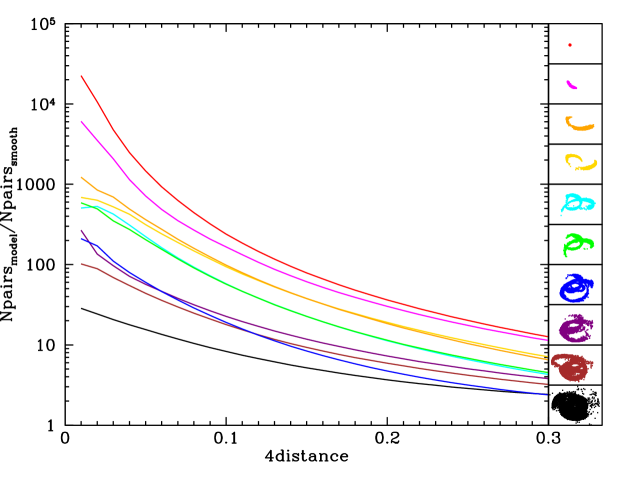
Figure 9: 4distance measurements for the Law & Majewski (2010) (LM10) model, where debris lost at each pericentric passage is shown in different colors. The ratio at each 4distance bin is calculated by dividing the number of pairs (determined by the 4distance metric, see Equation 1) in the data by the number of pairs in a smooth halo model (see Section 3.1 for details). The $x-z$ plot for each of LM10’s nine wraps are shown in the right hand panels. Starting at the top, these are: currently bound stars, stars lost on the most recent pericentric passage, stars lost on the next most recent passage, and so on.

Figure 10 shows substructure in the LM10 model observed with SEGUE’s pencil-beam geometry, again compared to a $\rho\propto r^{-3.5}$ smooth halo. The 4distance measurements follow the same general trend in the observed model as they do without the SEGUE footprint imposed, with only slight differences, indicating that while the survey footprint does add a complication to 4distance measurements, it does not do so in a drastic way. For this reason, however, we caution that we can only directly compare substructure measurements between samples observed with the same survey footprint. Bound stars indicate the highest possible level of substructure, while the lowest observable signal arises from the first wrap, which has had the most time to mix.

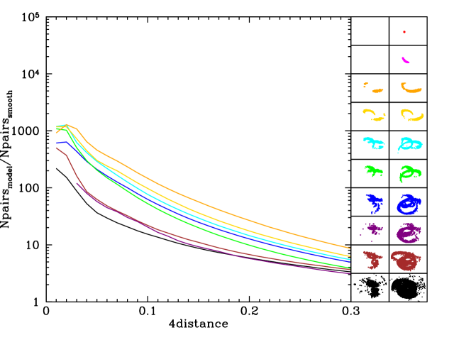
Figure 10: 4distance measurements for the LM10 model, but observed with the SEGUE footprint. The right hand panel shows the complete model, the middle panel the object in the SEGUE footprint, and the left hand panel the number of pairs compared to a smooth model for the objects in the SEGUE footprint.

3.3 Variation of substructure signal with model assumptions

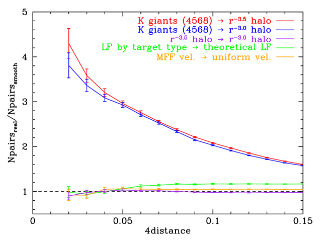
Figure 11: Substructure measurements for the full K giant sample, compared to two different model halos ($\rho\propto r^{-3.5}$, red; $\rho\propto r^{-3.0}$, blue). The purple, green, and orange lines show the effect of variations in assumptions on the overall 4distance measurement. The purple line shows a model $\rho\propto r^{-3.5}$ halo compared to a $\rho\propto r^{-3.0}$ halo, the green line shows the effect of using the observed luminosity function compared to a theoretical luminosity function, and the orange line shows the signal effect of using a Morrison et al. (1990) velocity ellipsoid with $(\sigma_{x},\sigma_{y},\sigma_{z})=(133,98,94)$ km s^-1 compared to a uniform velocity ellipsoid with $(\sigma_{x},\sigma_{y},\sigma_{z})=(100,100,100)$ km s^-1.

Figure 11 shows the result of our 4distance ratio measurement on the full K giant sample, against a number of smooth halo variations. We have measured a stronger substructure signal in K giants using our method with a smooth halo than using the same sample with S09’s shuffle method, because the smooth halo method allows for spatial clustering to contribute to the signal.

Tests of the various assumptions in our smooth halo model are depicted in Figure 11. The purple line shows the effect discussed above, where the centrally denser $\rho\propto r^{-3.5}$ halo has a amount of substructure not found in the $\rho\propto r^{-3.0}$ halo, which is roughly constant over the range of 4distance. Again, this effect is simply due to the fact that increased density leads to more measured pairs. The green line shows the effect caused by the choice of luminosity function. We have chosen to model the luminosity function (LF) by sampling the observed LF for each of our K giant target types, as opposed to using a theoretical LF for the relevant color range for each target type. This choice ensures that our smooth halo model has the same observational properties as the K giant sample. The green line shows that at small 4distance, there is no distinguishable difference between the two, but at larger 4distance, the observational LF counts more pairs than a theoretical LF. Finally, we show that the velocity ellipsoid, shown in orange, has a small effect as well. The cause of this effect is unclear, but could be due to the slightly narrower distributions in $\sigma_{y}$ and $\sigma_{z}$ in the Morrison et al. (1990) velocity ellipsoid. Fortunately the change in the 4distance ratio by each of these effects is much smaller than the total signal level in our real sample, as shown by the red and blue lines. We therefore disregard the effect of these assumptions in our final measurements.

Measuring a relatively strong signal using two different normalization methods confirms the presence of substructure in the K giant sample. Furthermore, a strong signal is produced when measured against two separate smooth halo models ($\rho\propto r^{-3.5}$, $\rho\propto r^{-3.0}$). As expected, the $\rho\propto r^{-3.5}$ measurement has a slightly weaker signal than the $\rho\propto r^{-3.0}$ measurement, due to the higher central density in the $\rho\propto r^{-3.5}$ halo, which increases the number of smooth pairs, driving down the overall measurement.

3.4 Friends-of-Friends

Determining a measurement of overall substructure in the halo is useful, but for certain purposes we would like to identify specific structures. Following S09, we use the 4distance in combination with a friends-of-friends (FoF) algorithm to obtain a local measure of substructure by linking stars into groups. These groups are stars with similar characteristics. In a metric system, two stars are associated if they are within a certain linking length, the maximum separation that two stars can have to be identified associated in a given metric. Recalling that a 4distance size contains information about sky position, velocity, and distance, it is useful to review what that means physically. Our chosen linking length of $4\delta=0.03$ corresponds to physical sizes in each dimension that can be found in Table 1.

FoF works by drawing a circle around each point, with a radius of one linking length. If the circle contains any other points, those points are in the group. Once a point is included in the group, a circle is drawn around it, and points inside that circle can now be added. The group is complete when no more points can be added. Since the 4distance involves more than just physical position, our circles need to be drawn in more than just spatial coordinates, but this highlights the power of the 4distance metric–the fact that it uses velocity information to find stars that are moving in the same direction.

Of additional concern when choosing a linking length is the pencil-beam geometry of the SEGUE survey. We want groups to extend across more than one plate pointing, but at the same time, we do not want the FoF algorithm to be too generous in linking spatial positions. In other words, while we desire the ability to connect nearby plate pointings, the deciding membership factor should be distance or velocity. Our choice of linking length of $4\delta=0.03$ takes these criteria into account. The maximum angular separation of 5.4^∘ allows for stars on nearby plate pointings to be included as possible group members, but will require them to have similar distances and velocities to be members of the same group. We will see below (Figure 16) that each Sgr stream wrap is mapped into a number of groups.

4 Results on Measuring Substructure in K giants

We have confirmed that the Milky Way halo is highly structured in K giants, but wish to make more meaningful conclusions about the nature of the halo. Given our large sample size compared to the previous K giant sample of S09, we are able to create subsamples that will allow us to explore both the inner and outer halo, as well as ranges in metallicity.

4.1 Variation with Galactocentric Radius

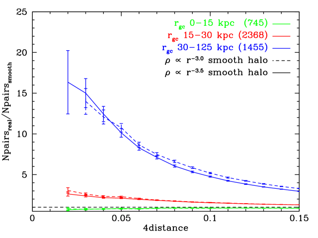
Figure 12: 4distance measurements for SEGUE K giants, divided into distance ranges in Galactocentric radius. The innermost subsample (shown in green), from $R_{gc}=0-15$ kpc, exhibits the least amount of substructure, while the outermost subsample (shown in blue), $R_{gc}>30$ kpc, shows the most. Red shows the subsample with $R_{gc}=15-30$ kpc. We also present two separate smooth halo normalizations in this figure ($R^{-3.0},R^{-3.5}$) in dashed and solid lines, respectively.

We might expect the inner halo to show less substructure than the outer halo for two reasons. First, any smooth component of the halo (formed, for example, by violent relaxation in the early stages of halo formation) would be found in the inner regions. Second, accreted stars will likely phase-mix faster in the inner halo due to the shorter dynamical times there. This expectation is largely borne out in the simulations of Bullock & Johnston (2005) and Cooper et al. (2010). In both papers the majority (but not all) of the realizations show more substructure in the outer than the inner halo (Xue et al., 2011; Cooper et al., 2011).

In our data we see substructure increasing monotonically with distance (see Figure 12), with the most distant stars (with $R_{gc}$ from 30 to 120 kpc) showing the strongest signal, $\sim$5 times more pairs than the halo stars with $R_{gc}$ between 15 and 30 kpc. While stars at these intermediate distances still show significant substructure, this is not the case for stars with $R_{gc}$ less than 15 kpc. However, there is abundant evidence for substructure in this region from other studies using either velocities (Schlaufman et al., 2009) or the full 6-D phase space information (e.g. Helmi et al., 1999). This highlights the fact that the 4distance is a relatively rough measurement of substructure.

4.2 Metallicity Dependence

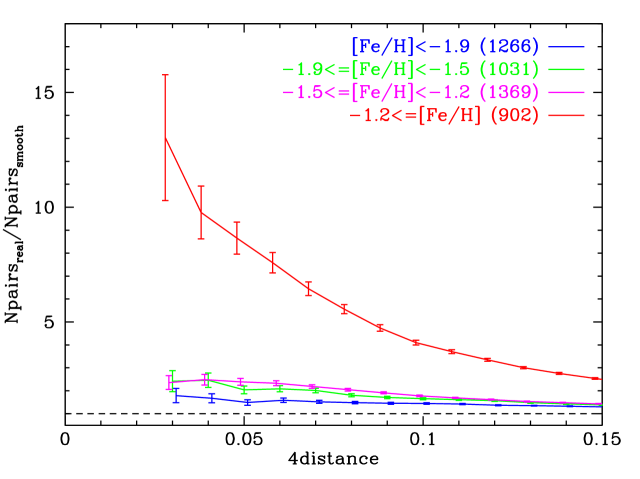
Figure 13: 4distance measurements for SEGUE K giants, divided into abundance ranges. The median metallicity of our K giant sample is [Fe/H] $\sim-1.5$. The red and blue lines represent the top and bottom 25% of the metallicity range, respectively. More metal-rich K giants show a high level of substructure, while the two metal-poor categories show similar, but lower, levels.

The use of K giants as tracers allows us to check explicitly for a dependence of substructure on metallicity, since it is considerably easier to obtain accurate [Fe/H] values for K giants than for BHB stars due to the much stronger metal lines in K giants. (Morrison et al, in preparation, demonstrate this for the SSPP metallicity measures.) This is of particular interest in the context of the disruption of accreted satellites into the field halo because of the mass-metallicity relation (Lee et al., 2006) which allows us to infer that if a low-mass object is accreted, its stars are likely to be metal-poor.

Figure 13 shows the global substructure measurement for the sample divided into [Fe/H] ranges. The most metal-rich group [Fe/H]$>-1.2$) shows a very strong substructure signal, with $\sim$ 8 times more pairs than a smooth halo at 4distance = 0.05. The two groups with intermediate metallicity ([Fe/H] between –1.2 and –1.9) have $\sim$ 2.5 times more pairs than the smooth halo at this value of 4distance, while the most metal-poor group ([Fe/H]$<-1.9$) shows the most subtle signal, with $\sim$ 50% more pairs than the smooth halo.

4.3 Comparison of BHB and K giant Substructure

We can use a comparison between BHB stars and K giants to investigate the properties of stellar populations of different age, because globular clusters with similar metallicity but blue horizontal branches are 1.5-2 Gyr older than those with red horizontal branches (Dotter et al., 2010). Because stars of all ages traverse the red giant branch, while only older stars of the same metallicity will become blue horizontal branch stars, any differences in substructure between the two samples is likely due to age.

Two photometric surveys have led to claims that BHB stars show less spatial substructure than the overall halo population. The first (Bell et al., 2008) counted numbers of main sequence turnoff stars in SDSS photometry covering distances from 7–35 kpc, and showed that there was significant substructure. (Deason et al., 2011) used a photometric technique to identify BHB stars in SDSS photometry, covering a distance range from 10–- 45 kpc, but using a different method and over spatial scales different from those in Bell et al. (2008). Each photometric method has weaknesses which may lead to them underestimating substructure: the distance measures to turnoff stars are not very accurate (Bell et al. estimate 0.9 mag. scatter) and this distance error will smooth out the “lumpiness” of spatial substructure along the line of sight. The BHB star sample suffers from some contamination by foreground blue stragglers of the halo, and since X11 show that the substructure in BHB stars increases with galactocentric distance, this too will have a smoothing effect on the amount of substructure. Thus, although it is clear that the photometric BHB sample of Deason et al. (2011) shows less substructure than the Bell et al. (2008) main sequence sample, it is not clear whether this is due to contamination of the BHB sample by inner halo blue stragglers or to an actual difference in substructure between the two tracers.

There is also some indirect evidence for a difference in substructure signal which is arrived at via a comparison with the models of Bullock & Johnston (2005). Bell et al. (2008) compared their spatial substructure method with the BJ05 models and found good overall agreement, while X11 compared the BHB substructure signal (in both velocity and position) with the same models and found less substructure than predicted by the models. However, since the two comparisons were made of a different signal (spatial vs spatial plus velocity) and over a different distance range (out to 35 vs 60 kpc), and we have seen that substructure in both BHB stars and K giants varies with distance, we feel that this result is not conclusive.

Clearly the spectroscopic samples of both BHB stars and K giants provide a safer measure of substructure, without the smoothing effects discussed above. Our original calculation of the amount of substructure in the K giant and BHB samples using the “shuffling” method of normalization (shown in Figure 7) showed significantly more substructure in the K giants. However, since substructure in both samples increases with galactocentric radius, a correct comparison will limit the K giant sample to the smaller distance range probed by the BHB stars. Figure 14 shows the result of this comparison: we see that the difference between the two stellar types has largely disappeared, and within the errors we see no significant difference in substructure using this method.

We thus see no conclusive evidence so far of different substructure signals in K giants and BHB star samples. It would be interesting to see a full analysis of both BHB and K giants using a smooth halo normalization as this would be more sensitive, because it also takes into account the spatial variation of numbers across the sky. In addition, more exploration of the relative contribution of BHB stars and K giants in the Sgr stream would be illuminating, but both are outside the scope of this work.

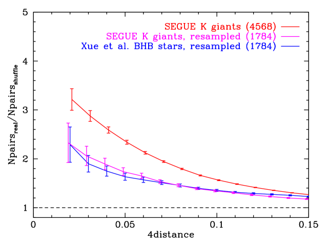
Figure 14: 4distance measurements for SEGUE K giants (magenta) and X11 BHB stars (blue), resampled to have matching distributions in $R_{gc}$. We also show the 4distance measurement for the intact K giant sample for reference (red). When resampled in this manner, K giants and BHBs show no significant evidence for differing amounts of kinematic substructure.

4.4 Distance or Metallicity?

Since the optical luminosity of a K giant increases as its metallicity decreases, a survey such as ours with a limiting magnitude will find only metal poor stars in the most distant regions, and only relatively metal-rich stars in its most nearby ones. We see in Figure 15 how the survey selection effects play into the distribution of distance and metallicity in our sample: the most metal rich stars cover a smaller distance range than the most metal poor ones.

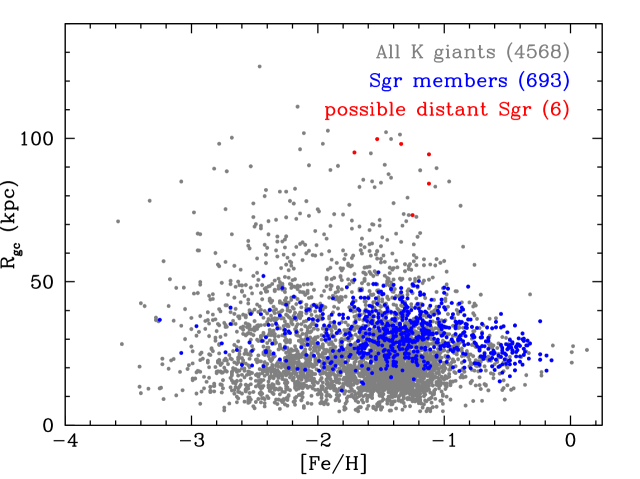
Figure 15: [Fe/H] vs distance for our K giant sample. The effects of SEGUE targeting and magnitude limits can be seen: there are no stars with [Fe/H]$>-0.7$ more distant than 50 kpc, while the most distant star has [Fe/H]$<-2.4$. Stars which are part of groups classified as ‘definitely’ belonging to Sgr (see Section 5 below) are shown with blue points, and stars belonging to a possible distant Sgr group are shown with red points.

If we saw more substructure in metal-poor and more distant stars we would need to worry about the above degeneracy, but in fact our results show the opposite behavior: the most metal-rich and the most distant stars show the most substructure.

We find that more metal rich stars have more substructure, but what does this imply for halo formation? Though its disruption is ongoing, the Sgr dwarf is a quite massive satellite (a recent estimate gives the current core mass at $\sim 5\times 10^{8}$ M_sun and intial virial mass at $\sim 1\times 10^{10}$ M_sun, placing Sgr among the most massive Local Group dwarf galaxies (see Mateo, 1998; Łokas et al., 2010) and has also been observed to be among the most metal-rich of the MW satellites (Mateo, 1998). Given that massive satellites are more metal-rich (see Lee et al., 2006), it seems likely that the large amount of metal-rich substructure in the sample can be attributed to Sgr, especially since we have taken pains to remove the disk from the sample and that Sgr is such a visible contributor to spatial substructure in the Field of Streams. It should be noted, however, that the other metallicity ranges do show a significant amount of substructure. We will attempt to quantify the contribution of Sgr and other streams to this substructure below.

5 FoF results

S09 find eight total groups, and only one group larger than two stars, which they suggest is associated with Sgr. Our results with a larger sample (4950 to their 101), yield a much larger number of groups; our data contain well over 100 groups larger than three members, and more than 20 groups larger than 10 members in size. About $38\%$ of our K giant sample is in a group of four or more members, $\sim 4\%$ is in a group with three members, and $\sim 8\%$ is in a group with two members (a pair). This then leaves $\sim 50\%$ not in a pair or a group. Of S09’s 101 stars, $\sim 14\%$ were in a pair, and only $\sim 5\%$ are found in a group of 4 or more stars, clearly illustrating that the power of the 4distance and FoF algorithm increases with sample size.

This large number of groups allows us to more deeply examine the properties of structures in the Milky Way halo. Significant group detections found via the FoF method can be found in Table 2. Figures 16 (groups with ten or more members) and 17 (groups with between four and nine members) show these groups in context in four dimensions of phase-space. The largest groups appear to be primarily associated with two large structures, one each in the Northern and Southern Galactic hemispheres. These are, respectively, the Sgr leading and trailing streams, which will be discussed in the next section. The diversity of substructure in the halo becomes more apparent in Figure 17, which shows smaller groups. Additionally, most of the groups in Figure 17 are located in the northern Galactic hemisphere.

Unfortunately, the FoF technique suffers from the same problem that afflicts the overall pair ratio measurement: there are more groups in regions with ($r_{\odot}\leq\sim 20$ kpc), due to the higher star density coupled with fixed linking length. In this case, this means that the regions that are relatively close to the Sun and Galactic center will appear to have more groups than more remote regions.

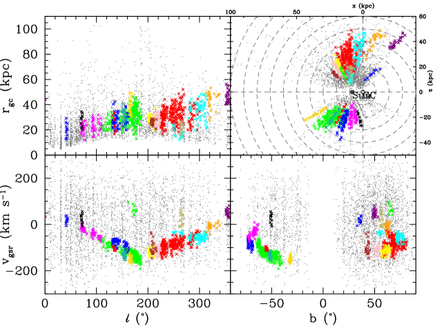
Figure 16: The FoF (friends-of-friends) groups greater than or equal to 10 members in size, shown with the line-of-sight velocity (corrected for the solar and LSR motion) $v_{gsr}$, against Galactic latitude $\sc{l}$ (lower left), Galactic latitude $b$ (lower right) and with longitude plotted against Galactocentric radius $R_{gc}$ (upper left). The upper right panel shows the $x-z$ plane, which is close to Sgr’s orbital plane. Dashed lines are every 10 kpc in $R_{gc}$. K giants are shown as colored crosses, with each color representing a different group (color repeats between groups should not be construed as an indication of group membership, but are merely caused by a limited number of colors). The full K giant sample is represented by gray dots in the background. Nearly all of these larger groups are associated with Sgr.

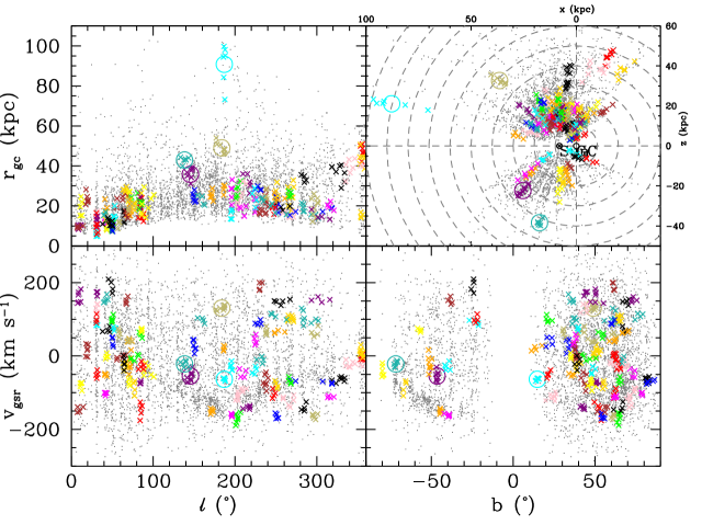
Figure 17: The FoF groups between 4 and 9 (inclusive) members in size, shown in 4 different sections of phase space as described in the caption for Figure 16. K giants are shown in colored crosses, with each color representing a different group (color repeats between groups should not be construed as an indication of group membership, but are merely caused by a limited number of colors). The full K giant sample is in greyscale in the background. The majority of these small groups fall in the northern Galactic hemisphere. Circled are the four notable non-Sgr substructure groups discussed in Section 5.2: gold, Orphan stream; purple and teal, Cetus Polar Stream; cyan, possible Sgr stream members at 90 kpc.

5.1 Attributing Groups to Known Substructure: Sgr

By comparing to models and observations, we can identify groups associated with known substuctures. The most important of these substructures is the Sgr stream. In fact, the Sgr stream can be seen clearly in a simple longitude-velocity plot even without using the FoF algorithm. Since Sgr streams dominate substructure in the Field of Streams and are the best-studied streams in the halo, we begin with quantifying their contribution to our sample. We need a reproducible technique to identify substructure belonging to Sgr, so we adopt the LM10 model as a way to define regions where Sgr streams should be observable, under the assumption that the LM10 models are an accurate representation of the spatial and kinematic properties of the Sgr streams. By observing the models using the SEGUE footprint (see Figure 18), we see the expected appearance of Sgr in a large–scale survey. In addition to LM10’s recommendation that only the five most recent pericentric passages are used, distance and velocity errors drawn from Gaussian distributions with sigma values of 20% and $\sim$ 5 km s^-1, respectively, have been added to each model point that falls within $1.49^{\circ}$ of a plate center. By constructing boxes around the observed model, we create the regions used to identify members of Sgr. We use a simple system to determine membership. There are boxes in four separate dimensions $(l-v_{gsr},b-v_{gsr},l-z_{gc},x_{gc}-z_{gc})$, shown in Figure 19. If 60% or more of a group’s stars fall into the box in all four plots, then the group is assigned to Sgr (referred to hereafter as “definitely Sgr”). A significant number of groups are identified as Sgr groups, and the majority of them have a large number of members, which means that the most obvious substructures in the halo are associated with Sgr. The width of the potential observed streams in the model is quite large, on the order of 10 kpc or 100 km s^-1, because Sgr is a massive dSph.

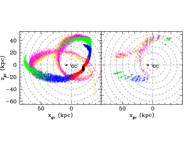
Figure 18: The LM10 model observed with SEGUE plate centers, shown in the $x_{gc}-z_{gc}$ plane, which is close to the Sgr orbital plane. In the left panel, each color represents stars lost on a different pericentric passage in the model (black shows bound stars; red, the most recent passage; blue, the next most recent passage; green, the second most recent; magenta, the third most recent; orange, the fourth most recent). The right panel shows the observed model, with the same colors. In both panels, dashed lines are every 10 kpc in $R_{gc}$.

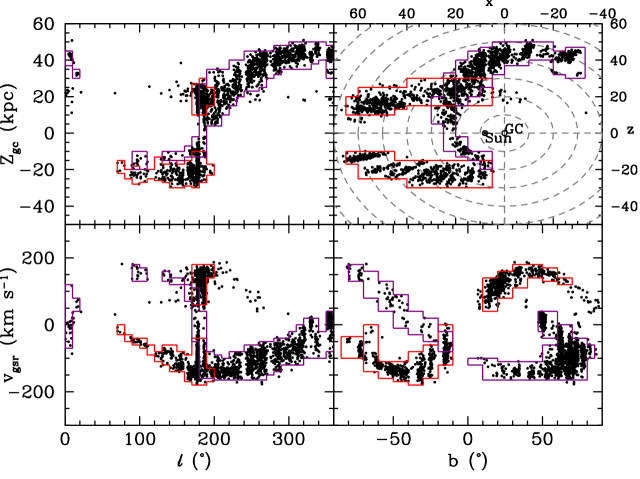
Figure 19: The regions defined as Sgr by use of the observed Law & Majewski (2010) model, shown with the line-of-sight velocity (corrected for the solar and LSR motion) $v_{gsr}$, against Galactic longitude $l$ (lower left), Galactic latitude $b$ (lower right) and with longitude plotted against Galactocentric height from the plane $z_{gc}$ (upper left). The upper right panel shows the $x-z$ plane, which is close to Sgr’s orbital plane. Dashed lines are every 10 kpc in $R_{gc}$. The observed model points are shown in black. The red boxes enclose streams identified as trailing in LM10, and the purple boxes enclose leading streams.

Figure 20 shows groups that are classified as “definitely Sgr,” which appear to have a narrower velocity distribution than the LM10 model, as well as a slightly different distance distribution, where observed stars appear to be on average closer to the Sun in some regions (notably in Figure 20 along the northern leading stream, where the average $R_{gc}$ differs by as much as 10 kpc, and the width of the velocity distribution is 50 km s^-1 narrower in some places). These groups are also largely consistent with the positions of the Sgr streams using SDSS K/M-giants in Yanny et al. (2009b), and using multiple target types by Koposov et al. (2012). The LM10 model largely reproduces the observed distribution of Sgr stars in both 2MASS (Majewski et al., 2003) and SDSS (Ruhland et al., 2011), pointing to a generally well constructed model. However, LM10 themselves acknowledge that their model does not produce features observed by SDSS (notably the bifurcation in the leading arm), so it is possible that other small deviations exist. Further observations are required to confirm Sgr membership and resolve these inconsistencies.

One of our smaller groups (six members; marked in cyan in Figure 17) has a large Galactocentric radius that is consistent with Newberg et al. (2003)’s detection of potential Sgr debris 90 kpc from the Galactic center at $(l,b)=(190^{\circ},30^{\circ})$. Debris is also found in this location by Ruhland et al. (2011), using a large sample of SDSS blue horizontal branch stars, as well as evidence of an extension to the trailing Sgr stream toward 90 kpc, for which we do not find FoF evidence. Further evidence for Sgr debris near this position was presented in Drake et al. (2013). Using RR Lyrae stars, Drake et al. (2013) find a structure, which they call the Gemini stream, located near $(l,b)=(195^{\circ},20^{\circ})$ and extending to a distance of $\sim 100$ kpc. All of these structures are located in or near the Sgr plane, though their radial velocities are unmeasured. The distant trailing stream hypothesis is further supported by observations presented in Belokurov et al. (2014), which found new Sgr trailing stream detections using photometry and kinematics in the Northern Galactic hemisphere. The results of Koposov et al. (2015) also support the distant trailing stream with spectroscopic observations of M giants in the area of the Galactic anticenter, consistent with the results of Drake et al. (2013) and Belokurov et al. (2014).

It has been proposed that NGC2419 (with $(l,b)=(180^{\circ},25^{\circ})$ and $v_{gsr}=-14$ km s^-1) is associated with this structure (Newberg et al., 2003), though the Gemini stream from Drake et al. (2013) is inconclusively linked to this cluster. Our FoF group has a position of $(l,b)=(187^{\circ},15^{\circ})$ and a $v_{gsr}$ of $-64$ km s^-1, making it possibly associated with either the Gemini stream or the Newberg et al. (2003) structure. The LM10 model does not predict debris in this position. Streams at large Galactocentric radius are likely lost on early passages, and are particularly important to constrain both Sgr’s accretion and the mass of the Milky Way.

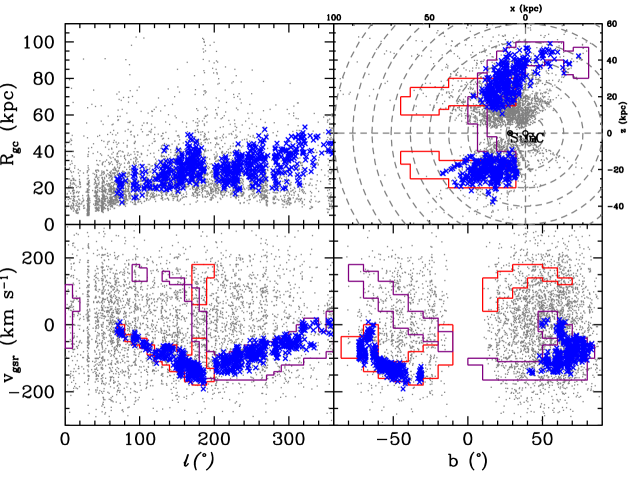
Figure 20: All stars classified as part of groups ‘definitely’ belonging to Sgr, shown in blue crosses. The panels are the same as those described in the caption for Figure 16. This classification is made by using the method described in section 5.1. The observed K giant substructure does not cover the extent of the LM10 model’s velocity prediction for the leading stream between $l=220^{\circ}$ and $l=360^{\circ}$.

5.2 Attributing Groups to Other Halo Substructure

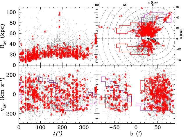
Figure 21: All groups classified as ‘definitely not’ belonging to Sgr. This classification is made by using the method described in section 5.1.

While Sgr is a significant component of the Milky Way halo, it is by no means the only visible substructure. Among the more interesting of other known substructures are the Orphan Stream (Belokurov et al., 2006), the Virgo Overdensity (Jurić et al., 2008), and Monoceros Ring (Belokurov et al., 2006); the Grillmair-Dionatos stream (Grillmair & Dionatos, 2006); and the Cetus Polar stream (Newberg et al., 2009). Our group classification catalog contains additional classifications beyond those for general Sgr/non-Sgr groups. These classifications are designed to identify groups potentially associated with the Orphan Stream and Cetus Polar Stream. Our choice of FoF linking length is not well suited to detecting some substructure; we are unlikely to find a group that covers the extent of the Virgo Overdensity due to its large spatial size. The Grillmair-Dionatos stream is quite narrow and relatively close; a linking length chosen to find substructure at a given distance will create larger groups at a closer distance and “wash out” narrow streams. Finally, our criteria for removing the disk from our sample makes it difficult for us to detect the Monoceros ring. Our selection boxes are designed in a similar manner to those for Sgr, but instead of using a model, we use observational data of the streams from SDSS detections (Newberg et al. (2009), Newberg et al. (2010)).

We identify several relatively large groups that are candidates for Orphan Stream and Cetus Polar Stream membership, with velocities and distances consistent with observations in Newberg et al. (2010), and Newberg et al. (2009) and Koposov et al. (2012), respectively. These groups represent a small fraction of our overall sample, but are likely to be members of the Orphan and Cetus Polar streams. Aside from their matching kinematic data, the groups have [Fe/H] consistent with observations for each stream. Interestingly, both the Orphan and Cetus Polar streams are spatially coincident with Sgr in portions of the sky, so finding these groups is an illustration of the power of the FoF algorithm combined with 4-dimensional spatial and kinematic data. These groups are marked in Figure 17.

We find one high latitude distant group that is spatially coincident with Sgr (group 397), and at roughly the same distance, but which has a strikingly different $v_{gsr}$ ($\Delta v\approx 200$ km s^-1). While this group has $(l,b)$ and $v_{gsr}$ consistent with observed substructure in Virgo (Newberg et al., 2007), it has a much greater distance. That this group may be associated with debris lost on an early pericentric passage of Sgr. In a future paper in this series (Z. Ma et al., in preparation), we further investigate this group.

Other groups listed in Table 2 may belong to known substructures. Two groups with $l\approx 260^{\circ}$ and $b\approx 60^{\circ}$ (group 220 and group 211) have stars with $v_{gsr}$ consistent with the Virgo Stellar Stream (Duffau et al., 2006), but are over 10 degrees from the observed stream, and could be possible extensions to the Virgo Stellar Stream. We also detect a number of possible members of the Virgo Overdensity. In particular, groups 175 and 293 share the spatial and kinematic properties of the Virgo Overdensity (Bonaca et al., 2012). We will also further examine these stars, and in particular their [$\alpha$/Fe] properties, in Z. Ma et al. (in preparation).

Three groups with $l<45^{\circ}$ are located near the Galactic center with a large range of $v_{gsr}$. Their origin is unclear, but they could be associated with the Hercules-Aquila cloud (Belokurov et al., 2007).

Grillmair (2014) recently reported the discovery of two new halo streams, named Hermus and Hyllus. We find a group of five stars near the location of these streams (group 483). Further investigation of these streams and the members of the group are needed to conclusively determine their membership.

Koposov et al. (2014) discovered a new metal poor stream in the ATLAS survey at a distance of 20 kpc, though it is mostly outside the SDSS footprint. Finally, Martin et al. (2014) find a number of new streams in the vicinity of the Andromeda and Triangulum Galaxies using the PAndAS survey. Both of these locations are near the edge of our Milky Way disk star exclusion cuts, so we find no groups related to these streams.

We provide the full catalog of stars in groups with 4 members or larger in Table 3.

5.3 FoF Discussion

5.3.1 False positives

A number of false positive groups are expected because our choice of linking length does not change with $R_{gc}$. These false positive groups occur especially in the inner halo due to its higher density. In a smooth halo, we know that any identified groups are simply chance groupings of stars with similar positions, velocities, and distances. With a sample of stars, however, we expect there to be larger groups, consistent with the clustering of stars in substructure. For a data sample and a smooth halo model of equivalent size, we expect to find both a smaller number of total stars in groups and a smaller average group size in the smooth halo model than in the strucutred data sample.

We have computed the expected number of groups in a smooth halo by generating ten model smooth halos, as described in section 3.1 above. We find that averaged over the ten halos, we expect to find $\sim 1600$ stars in groups with an average group size of 2.6, compared to $\sim 2200$ stars in groups in our K giant sample with an average group size of 4, leading to a higher average number of stars per group in the K giant sample by 1.4. These numbers are even more drastic when considering groups of three or more members, where there are 1550 stars in groups in the K giant sample, but only 800 stars in groups averaged over the ten smooth halo models, a factor of nearly two. We can conclude that a large fraction of our small groups (with a size of 3 members or less) are likely to be chance pairings and therefore false positives, but the fraction of these false positive groups decreases with group size.

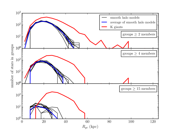
Figure 22: Number of stars in groups as a function of Galactocentric radius, for both the K giant sample and for model smooth halos. Red lines show the number of stars in groups for the K giant sample, black lines show the number of stars in groups for each of ten individual smooth halo models. The blue line shows the average number of stars in groups for the smooth halo models. Top panel: All stars in groups of any size (two or more members). Middle panel: Stars in groups of four or more members. Bottom panel: Stars in groups of ten or more members. In all cases, there are more total groups in the K giant sample than on average in the smooth halo models.

In addition, we have computed the number of stars in groups as a function of Galactocentric radius for a number of group sizes. We show the results of this analysis in Figure 22. In the top panel of Figure 22 we see that the number of stars in groups in the smooth halo models (blue line) is significant, but not as large as the number of stars in groups in the K giant sample at any Galactocentric radius, by at least a factor of two at most radii. There are almost no falsely grouped stars at radii greater than 40 kpc. The trend continues for groups of larger size as well, with groups of four members or more and groups of ten members or more showing significantly more stars in groups at all but the most nearby Galactocentric radii.

It is also possible for our method to miss cold substructure (e.g., the Grillmair-Dionatos stream; Grillmair & Dionatos, 2006) in the higher density inner regions of the halo, because our choice of linking length are designed to identfy cold substructure in more distant regions of the halo. In effect, because of the higher stellar density, more pairs per star will be found, increasing a group’s size and the range of its values in the 4-dimensional parameter space, and “washing out” the cold stream.

5.3.2 Group membership trends

Figure 23 shows a histogram of the number of groups with a given group size and their classifications. While the largest groups (larger than 10 members) are predominantly classified as Sgr, the smallest groups (10 or fewer members) are mostly unlikely to be Sgr, and only 13% of all groups are likely to be members of any previously known substructure.

We can, therefore, give limits on the fraction of halo stars residing in substructure. At least 50% of K giants in our sample show no detection of substructure. Additionally, at least 13% of stars in our sample are members of Sgr, and roughly 1% of stars are members of other known substructure. The remaining $\sim 36$% of stars in the sample comprise previously undiscovered substructure.

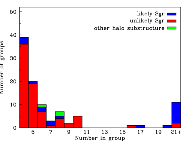
Figure 23: Number of groups at a given group size, classified by their associated structure. Blue are groups within Sgr regions, green and red are groups within non-Sgr regions. The rightmost bin is the combination of all groups larger than 20 members: the largest group contains 255 stars. For groups larger than 20 members, 80% of groups are associated with Sgr. Overall, approximately 700 stars are associated with Sgr.

Figure 24 shows the fraction of stars in groups that belong to Sgr groups as a function of $R_{gc}$ in different samples of K giants. For the full K giant sample, we see that about 1/3 of stars in groups belong to a Sgr group, and at least 50% of stars with $R_{gc}>$ 30 kpc are Sgr members. This trend also helps to explain our earlier finding of an increase in substructure with $R_{gc}$, as Sgr is a greater percentage of the total stellar population as $R_{gc}$ increases. The Figure also shows four metallicity selected samples. It is clear from this diagram that in the more metal poor samples, there is a smaller fraction of Sgr stars than in the more metal rich samples. In fact, for some $R_{gc}$ bins, Sgr represents more than 75% of the stars. Since the Sgr stream is by far the dominant structure found in our analysis, this result readily explains the trend of increasing substructure with metallicity, and much of the inner/outer halo differences found in Section 4. This conclusion also suggests an alternate explanation for the lower level of substructure found by X11 and Cooper et al. (2011) in BHB stars compared to the simulations: not age, but metallicity. Metallicity plays into substructure detection via the mass-metallicity relation: more massive satellites contain more metal-rich stars and are also easier to detect in pencil-beam surveys such as SEGUE because of the higher stellar density in their streams. Stars from low-mass satellites will be metal-poor and hard to detect because of their lower stellar density and the wide spacing of the SEGUE fields.

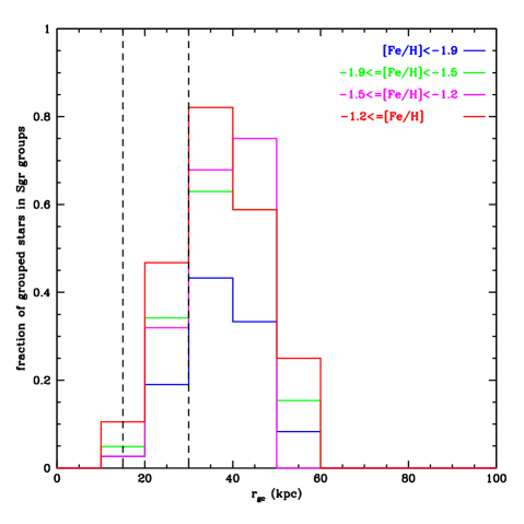
Figure 24: Fraction of stars in groups associated with Sgr as a function of Galactocentric radius. The colored lines show different metallicity samples discussed in Section 4.2. Dashed vertical lines indicate the distance ranges over which we divide our sample into $R_{gc}$ bins in Figure 12. Approximately 1/3 of stars in groups are associated with Sgr, and the most metal rich sample is largely composed of Sgr stars.

6 Conclusions

We use a sample of 4568 halo K giants with distances up to 125 kpc to measure substructure in the halo using a metric sensitive to both spatial and kinematical substructure. This sample complements and extends the work of X11 and Cooper et al. (2011) on substructure in large samples of BHB stars because K giants are not restricted to old, metal poor populations.

Outer halo K giants show more substructure than inner halo ones, in agreement with the results of X11 and Cooper et al. (2011). In addition, we find that the most metal-rich K giants in our sample (with [Fe/H] $\geq-1.2$) show the most substructure of all the K giants. In addition, when directly comparing the amount of substructure in the BHB sample from X11 and the K giants presented in this work, we find no significant difference between the two samples when selecting stars over equivalent distance ranges. Further work is needed to fully understand the contribution of BHBs and K giants to the Galactic stellar halo.

Since Sgr stream stars are on average more metal rich than the rest of the halo and the Sgr stream is not found in the inner halo, we investigated the possibility that the Sgr stream is responsible for both trends in substructure (metallicity and distance). We find that for stars with [Fe/H] greater than –1.9, most of the groups with $R_{gc}$ greater than 30 kpc belong to the Sgr stream, and conclude that in the case of the Milky Way, the Sgr stream is responsible for the increase of substructure with both metallicity and distance.

Table 2: Selected FoF groups found at linking length $4\delta=0.03$

Group ID	Members	$l$	$b$	$v_{gsr}$	$R_{gc}$	[Fe/H]	Notes
		deg	deg	km s-1	kpc	dex
3	212	251.48	68.18	-85.77	31.98	-1.39	Sgr
11	174	162.10	-53.62	-123.26	30.55	-1.19	Sgr
41	59	143.72	-70.97	-80.86	27.38	-1.30	Sgr
28	54	300.51	74.36	-56.40	36.15	-1.34	Sgr
40	50	88.08	-67.66	-34.97	22.65	-1.21	Sgr
210	34	208.45	60.65	-115.48	27.93	-1.48	Sgr
369	27	217.83	52.33	-109.82	27.68	-1.18	Sgr
9	24	340.01	49.86	49.85	46.70	-1.49	unlikely Sgr
5	23	323.22	62.38	-7.61	43.89	-1.18	Sgr
110	21	153.98	-51.47	-133.08	31.16	-1.24	Sgr
107	20	209.58	43.17	-98.98	25.61	-1.34	likely Sgr
376	17	166.29	-31.85	-149.72	39.24	-1.26	Sgr
220	16	264.95	56.62	24.56	20.24	-1.79	unlikely Sgr
332	10	71.63	-50.49	25.61	27.75	-1.41	not Sgr
124	10	135.13	-54.99	-105.92	25.55	-1.39	unlikely Sgr
211	10	172.49	65.68	64.95	20.36	-1.28	unlikely Sgr
71	10	42.12	35.69	18.20	20.34	-1.59	possible Hercules-Aquila Cloud
222	10	258.33	55.49	-35.96	17.24	-1.39	unlikely Sgr
26	9	43.57	35.84	-148.32	12.81	-1.55	possible Hercules-Aquila Cloud
175	8	288.81	60.93	103.14	17.72	-1.34	possible Virgo Overdensity
32	8	145.52	-46.47	-54.29	35.85	-2.13	Cetus Polar Stream
408	8	183.93	48.88	130.70	49.07	-2.11	Orphan Stream
275	7	328.32	82.11	-63.96	36.37	-1.34	Sgr
261	6	41.88	78.69	-101.72	12.14	-1.57	possible Hercules-Aquila Cloud
388	6	187.08	14.80	-63.43	90.80	-1.34	possible distant Sgr
224	6	138.39	-71.76	-21.53	42.94	-2.19	Cetus Polar Stream
8	6	355.33	51.05	5.53	43.92	-1.82	Sgr
397	5	256.07	69.40	148.04	20.05	-1.22	possible older Sgr
483	5	77.21	45.34	-4.32	23.80	-1.66	possible Hermus/Hyllus
93	4	304.25	73.51	153.35	15.10	-1.59	possible Virgo Overdensity

Table 3: Group catalog: K giants sorted by group for groups with 4 or more members

Plate	MJD	Fiber	$l$	$b$	$v_{gsr}$	$v_{err}$	$d$	$d_{err}$	[Fe/H]	$g_{01}$	$M_{r}$	$r_{gc}$	Target	Group	Group
			deg	deg	km s-1	km s-1	kpc	kpc	dex	mag	mag	kpc	type	ID	flag
519	52283	62	289.4253	64.0776	-48.7	1.4	37.2	4.2	-0.81	17.027	-1.98	36.862	3	3	6
2413	54169	215	246.7213	60.4712	-89.2	2.6	41.5	6.5	-1.02	18.665	-0.13	43.808	1	3	6
2509	54180	597	237.3916	74.4764	-105.9	1.6	35.4	4.2	-1.22	17.310	-1.30	37.449	2	3	6
2857	54453	5	231.0205	67.2724	-101.0	1.5	21.8	2.4	-1.52	15.808	-1.77	24.995	4	3	6
2857	54453	177	228.0546	66.8574	-112.3	2.7	17.2	2.5	-2.52	16.289	-0.50	20.832	1	3	6

Note. — Table 3 is published in its entirety in the electronic edition of ¡¿. A portion is shown here for guidance regarding its form and content.

References

- Ahn et al. (2012) Ahn, C. P., Alexandroff, R., Allende Prieto, C., et al. 2012, ApJS, 203, 21
- Bell et al. (2008) Bell, E. F., Zucker, D. B., Belokurov, V., et al. 2008, ApJ, 680, 295
- Bell et al. (2010) Bell, E. F., Xue, X. X., Rix, H.-W., Ruhland, C., & Hogg, D. W. 2010, AJ, 140, 1850
- Belokurov et al. (2006) Belokurov, V., Zucker, D. B., Evans, N. W., et al. 2006, ApJ, 642, L137
- Belokurov et al. (2007) Belokurov, V., Evans, N. W., Bell, E. F., et al. 2007, ApJ, 657, L89
- Belokurov et al. (2007) Belokurov, V., Evans, N. W., Irwin, M. J., et al. 2007, ApJ, 658, 337
- Belokurov et al. (2014) Belokurov, V., Koposov, S. E., Evans, N. W., et al. 2014, MNRAS, 437, 116
- Binney & Merrifield (1998) Binney, J. and Merrifield, M. 1998, Galactic Astronomy, Princeton University Press, Princeton NJ
- Bonaca et al. (2012) Bonaca, A., Jurić, M., Ivezić, Ž., et al. 2012, AJ, 143, 105
- Bovy et al. (2012) Bovy, J., Rix, H.-W., Liu, C., et al. 2012, ApJ, 753, 148
- Bullock & Johnston (2005) Bullock, J. S., & Johnston, K. V. 2005, ApJ, 635, 931
- Carney et al. (1996) Carney, B. W., Laird, J. B., Latham, D. W., & Aguilar, L. A. 1996, AJ, 112, 668
- Carollo et al. (2010) Carollo, D., Beers, T. C., Chiba, M., et al. 2010, ApJ, 712, 692
- Carraro et al. (2010) Carraro, G., Vázquez, R. A., Costa, E., Perren, G., & Moitinho, A. 2010, ApJ, 718, 683
- Cooper et al. (2010) Cooper, A. P., Cole, S., Frenk, C. S., et al. 2010, MNRAS, 406, 744
- Cooper et al. (2011) Cooper, A. P., Cole, S., Frenk, C. S., & Helmi, A. 2011, MNRAS, 417, 2206
- Deason et al. (2011) Deason, A. J., Belokurov, V., & Evans, N. W. 2011, MNRAS, 416, 2903
- Diemand et al. (2007) Diemand, J., Kuhlen, M., & Madau, P. 2007, ApJ, 667, 859
- Dotter et al. (2010) Dotter, A., Sarajedini, A., Anderson, J., et al. 2010, ApJ, 708, 698
- Drake et al. (2013) Drake, A. J., Catelan, M., Djorgovski, S. G., et al. 2013, ApJ, 765, 154
- Duffau et al. (2006) Duffau, S., Zinn, R., Vivas, A. K., et al. 2006, ApJ, 636, L97
- Eisenstein et al. (2011) Eisenstein, D. J., Weinberg, D. H., Agol, E., et al. 2011, AJ, 142, 72
- Fermani & Schönrich (2013) Fermani, F., & Schönrich, R. 2013, MNRAS, 432, 2402
- Font et al. (2011) Font, A. S., McCarthy, I. G., Crain, R. A., et al. 2011, MNRAS, 416, 2802
- Fukugita et al. (1996) Fukugita, M., Ichikawa, T., Gunn, J. E., et al. 1996, AJ, 111, 1748
- Geisler (1984) Geisler, D. 1984, PASP, 96, 723
- Grillmair (2014) Grillmair, C. J. 2014, ApJ, 790, L10
- Grillmair & Dionatos (2006) Grillmair, C. J., & Dionatos, O. 2006, ApJ, 643, L17
- Gorski et al. (1989) Gorski, K. M., Davis, M., Strauss, M. A., White, S. D. M., & Yahil, A. 1989, ApJ, 344, 1
- Gunn et al. (2006) Gunn, J. E., Siegmund, W. A., Mannery, E. J., et al. 2006, AJ, 131, 2332
- Harding et al. (2001) Harding, P., Morrison, H. L., Olszewski, E. W., et al. 2001, AJ, 122, 1397
- Helmi et al. (1999) Helmi, A., White, S. D. M., de Zeeuw, P. T., & Zhao, H. 1999, Nature, 402, 53
- Helmi et al. (2011) Helmi, A., Cooper, A. P., White, S. D. M., et al. 2011, ApJ, 733, L7
- Ibata et al. (1994) Ibata, R. A., Gilmore, G., & Irwin, M. J. 1994, Nature, 370, 194
- Johnston et al. (1996) Johnston, K. V., Hernquist, L., & Bolte, M. 1996, ApJ, 465, 278
- Jurić et al. (2008) Jurić, M., Ivezić, Ž., Brooks, A., et al. 2008, ApJ, 673, 864
- Koposov et al. (2012) Koposov, S. E., Belokurov, V., Evans, N. W., et al. 2012, ApJ, 750, 80
- Koposov et al. (2014) Koposov, S. E., Irwin, M., Belokurov, V., et al. 2014, MNRAS, 442, L85
- Koposov et al. (2015) Koposov, S. E., Belokurov, V., Zucker, D. B., et al. 2015, MNRAS, 446, 3110
- Law & Majewski (2010) Law, D. R., & Majewski, S. R. 2010, ApJ, 714, 229
- Lee et al. (2006) Lee, H., Skillman, E. D., Cannon, J. M., et al. 2006, ApJ, 647, 970
- Lee et al. (2008) Lee, Y. S., Beers, T. C., Sivarani, T., et al. 2008, AJ, 136, 2022
- Łokas et al. (2010) Łokas, E. L., Kazantzidis, S., Majewski, S. R., et al. 2010, ApJ, 725, 1516
- Lynden-Bell & Lynden-Bell (1995) Lynden-Bell, D., & Lynden-Bell, R. M. 1995, MNRAS, 275, 429
- Majewski (1993) Majewski, S. R. 1993, ARA&A, 31, 575
- Majewski et al. (2003) Majewski, S. R., Skrutskie, M. F., Weinberg, M. D., & Ostheimer, J. C. 2003, ApJ, 599, 1082
- Martin et al. (2014) Martin, N. F., Ibata, R. A., Rich, R. M., et al. 2014, ApJ, 787, 19
- Mateo et al. (1996) Mateo, M., Mirabal, N., Udalski, A., et al. 1996, ApJ, 458, L13
- Mateo (1998) Mateo, M. L. 1998, ARA&A, 36, 435
- Mathewson et al. (1974) Mathewson, D. S., Cleary, M. N., & Murray, J. D. 1974, ApJ, 190, 291
- Morrison et al. (1990) Morrison, H. L., Flynn, C., & Freeman, K. C. 1990, AJ, 100, 1191
- Morrison et al. (2000) Morrison, H. L., Mateo, M., Olszewski, E. W., et al. 2000, AJ, 119, 2254
- Morrison et al. (2003) Morrison, H. L., Norris, J., Mateo, M., et al. 2003, AJ, 125, 2502
- Newberg et al. (2003) Newberg, H. J., Yanny, B., Grebel, E. K., et al. 2003, ApJ, 596, L191
- Newberg et al. (2007) Newberg, H. J., Yanny, B., Cole, N., et al. 2007, ApJ, 668, 221
- Newberg et al. (2009) Newberg, H. J., Yanny, B., & Willett, B. A. 2009, ApJ, 700, L61
- Newberg et al. (2010) Newberg, H. J., Willett, B. A., Yanny, B., & Xu, Y. 2010, ApJ, 711, 32
- Norris et al. (1985) Norris, J., Bessell, M. S., & Pickles, A. J. 1985, ApJS, 58, 463
- Preston et al. (1991) Preston, G. W., Shectman, S. A., & Beers, T. C. 1991, ApJ, 375, 121
- Reylé et al. (2009) Reylé, C., Marshall, D. J., Robin, A. C., & Schultheis, M. 2009, A&A, 495, 819
- Ruhland et al. (2011) Ruhland, C., Bell, E. F., Rix, H.-W., & Xue, X.-X. 2011, ApJ, 731, 119
- Schlaufman et al. (2009) Schlaufman, K. C., Rockosi, C. M., Allende Prieto, C., et al. 2009, ApJ, 703, 2177
- Schlegel et al. (1998) Schlegel, D. J., Finkbeiner, D. P., & Davis, M. 1998, ApJ, 500, 525
- Schlesinger et al. (2012) Schlesinger, K. J., Johnson, J. A., Rockosi, C. M., et al. 2012, ApJ, 761, 160
- Skrutskie et al. (2006) Skrutskie, M. F., Cutri, R. M., Stiening, R., et al. 2006, AJ, 131, 1163
- Smee et al. (2013) Smee, S. A., Gunn, J. E., Uomoto, A., et al. 2013, AJ, 146, 32
- Springel et al. (2008) Springel, V., Wang, J., Vogelsberger, M., et al. 2008, MNRAS, 391, 1685
- Starkenburg et al. (2009) Starkenburg, E., Helmi, A., Morrison, H. L., et al. 2009, ApJ, 698, 567
- Vivas & Zinn (2006) Vivas, A. K., & Zinn, R. 2006, AJ, 132, 714
- Xue et al. (2008) Xue, X. X., Rix, H. W., Zhao, G., et al. 2008, ApJ, 684, 1143
- Xue et al. (2011) Xue, X.-X., Rix, H.-W., Yanny, B., et al. 2011, ApJ, 738, 79
- Xue et al. (2014) Xue, X.-X., Ma, Z., Rix, H.-W., et al. 2014, ApJ, 784, 170
- Yanny et al. (2009a) Yanny, B., Rockosi, C., Newberg, H. J., et al. 2009, AJ, 137, 4377
- Yanny et al. (2009b) Yanny, B., Newberg, H. J., Johnson, J. A., et al. 2009, ApJ, 700, 1282
- York et al. (2000) York, D. G., Adelman, J., Anderson, J. E., Jr., et al. 2000, AJ, 120, 1579
- Zinn (1985) Zinn, R. 1985, ApJ, 293, 424