Multiscale asymptotic homogenization analysis
of thermo-diffusive composite materials

Abstract

In this paper an asymptotic homogenization method for the analysis of composite materials with periodic microstructure in presence of thermodiffusion is described. Appropriate down-scaling relations correlating the microscopic fields to the macroscopic displacements, temperature and chemical potential are introduced. The effects of the material inhomogeneities are described by perturbation functions derived from the solution of recursive cell problems. Exact expressions for the overall elastic and thermodiffusive constants of the equivalent first order thermodiffusive continuum are derived. The proposed approach is applied to the case of a two-dimensional bi-phase orthotropic layered material, where the effective elastic and thermodiffusive properties can be determined analytically. Considering this illustrative example and assuming periodic body forces, heat and mass sources acting on the medium, the solution performed by the first order homogenization approach is compared with the numerical results obtained by the heterogeneous model.

Keywords: Periodic microstructure, Asymptotic homogenization, Thermodiffusion, Overall material properties.

1 Introduction

Composite materials are extensively used in industrial practice. Indeed, many advanced engineering applications, such as aerospace, aircraft, green building, biomedical, energetics and electronics require the design and the use of heterogeneous multiphase materials. Due to the microstructural effects as well as the interaction between their constituents, these materials may present several favorable physical properties, as for example high stiffness, improved strength and toughness, enhanced thermal conductivity, mass diffusivity or electrical permittivity.

Recently, multiphase composite materials have been largely used in the design and fabrication of battery devices, in particular of lithium-ion batteries and solid oxide fuel cells (Nakajo et al., 2012; Dev et al., 2014; Ellis et al., 2012). Since high operational temperatures can be reached and intense particle fluxes are needed for maintaining the electrical current, the components of such battery devices are subject to severe thermomechanical stresses as well as stresses induced by the particle diffusion, which can cause damage and crack formation, compromising the performance of the devices in terms of power generation and energy conversion efficiency (Atkinson and Sun, 2007; Delette et al., 2013). Modelling the mechanical and thermodiffusive properties of the components of such battery devices represent a crucial issue in order to predict these phenomena and then to ensure the successful manufacture and the reliability of the systems.

The macroscopic behavior of thermodiffusive composite materials used for realizing lithium-ion batteries and solid oxide fuel cells is influenced by multiphysics phenomena occurring at scale-lengths characteristic of the microscopic constituents, which is small compared to the macroscopic dimension (i.e. structural size) (Richardson et al., 2012; Bove and Ubertini, 2008; Hajimolana et al., 2011). Consequently, multiscale techniques represent an appropriate and powerful tool for modelling the effects of the microstructures on the macroscopic mechanical and thermodiffusive properties of these materials. In particular, for composites with periodic microstructures, homogenization techniques represent an useful and advantageous method for providing a rigorous and synthetic description of the effects of the microscopic phases on the overall properties of the materials. The application of these approaches makes possible to avoid the challenging numerical computations required by computational modelling of heterogeneous media.

Several homogenization techniques have been proposed for studying overall static and dynamic elastic properties of composite materials with periodic microstructures, such as the asymptotic (see for example Bensoussan et al. (1978); Bakhvalov and Panasenko (1984); Gambin and Kroner (1989); Allaire (1992); Boutin and Auriault (1993); Meguid and Kalamkarov (1994); Boutin (1996); Andrianov et al. (2008); Tran et al. (2012)), the variational-asymptotic methods (see for example Smyshlyaev and Cherednichenko (2000); Peerlings and Fleck (2004); Smyshlyaev (2009); Bacigalupo (2014); Bacigalupo and Gambarotta (2014)) and the computational approaches (see for example Forest and Sab (1998); Forest (2002); Kouznetsova et al. (2002, 2004); Kaczmarczyk et al. (2008); Forest and Trinh (2011); Bacigalupo and Gambarotta (2010, 2011, 2013); De Bellis and Addessi (2011); Addessi et al. (2013); Bacca et al. (2013a, b, c)). These techniques associate to the considered heterogeneous material at the micro-scale, described by a standard Cauchy continuum, an equivalent homogenous medium at the macro-scale. The behavior of the equivalent macroscopic material can be described by means of a first order continuum or alternatively a non-local medium. Multiscale asymptotic and computational homogenization procedures have been also proposed for the analysis of heterogeneous media in presence of multiphysics phenomena, such as thermomechanical (Kanouté et al., 2009; Zhang et al., 2007; Aboudi et al., 2001) and thermo-magneto-electro-elastic (Sixto-Camacho et al., 2013) deformations. Recently, these methods have been applied for studying the influence of the microstructural effects on the macroscopical mechanical behavior and operative performances of lithium-ion batteries (Salvadori et al., 2014) and solid oxide fuel cells (Bacigalupo et al., 2014). The overall properties of periodic multilayered structures characterizing such energy devices can be efficiently described by means of homogenization methods developed for periodic composite materials. Nevertheless, to the author’s knowledge, a rigorous asymptotic procedure accounting for the effects of the microstructures on both macroscopic elastic and thermodiffusive properties of composite materials as well as on the coupling between these properties is still unknown in literature.

In this paper, an original asymptotic homogenization method for modelling the static elastic, thermal and diffusive properties of periodic thermodiffusive composite materials is proposed. The rigorous approach developed in Bakhvalov and Panasenko (1984); Smyshlyaev and Cherednichenko (2000); Bacigalupo (2014) and Bacigalupo and Gambarotta (2014) is extended in order to account for the effects of the microstructures on the macroscopic temperature and chemical potential of the materials and on the stresses induced by these fields. The displacements, temperature and chemical potential at the micro- and macro-scale are related through an asymptotic expansion of the microscopic fields in terms of characteristic size $\varepsilon$ of the microstructure. This expansion depends both on the macroscopic strains, temperature and chemical potential gradients and on unknown perturbation functions accounting for the effects of the heterogeneities. Perturbation functions representing the effects of the material microstructures on the displacement, temperature, chemical potential and on the coupling effects between these fields are introduced. These perturbation functions, depending only on the properties of the microstructure, are obtained through the solution of non-homogeneous problems on the cell with periodic boundary conditions.

Similarly to the procedure proposed in Smyshlyaev and Cherednichenko (2000) and Bacigalupo (2014), averaged field equations of infinite order are obtained, and their formal solution is performed by representing the macroscopic displacements, temperature and chemical potential in terms of power series. Field equation for the homogenized first order thermodiffusive continuum are derived, and exact expressions for the overall elastic and thermodiffusive constants of this equivalent medium are obtained. The proposed formulation is applied to the case of a two-dimensional bi-phase orthotropic layered material. The effective elastic and thermodiffusive constants corresponding to this example are determined analytically using the general expressions derived by the homogenization procedure. The solution performed by the proposed approach is compared with the numerical results obtained by the heterogeneous model assuming periodic body forces, heat and mass sources acting on the considered bi-phase layered composite.

The article is organized as follows: in Section 2 the geometry of the considered thermodiffusive composite material with periodic microstructure is illustrated, and the corresponding constitutive relations and balance equations are introduced. The developed multiscale asymptotic homogenization technique is described in Section 3, based on down-scaling relations correlating the microscopic fields to the macroscopic displacements, temperature and chemical potential. The unknown perturbation functions describing the effects of the material heterogeneities are defined as solutions of the corresponding non-homogeneous cell problems. In the same Section, averaged field equations of infinite order are obtained, and a solution scheme based on asymptotic expansion of the macroscopic displacements, temperature and chemical potential field is reported. Field equations and explicit expressions for the overall elastic and thermodiffusive constants of the equivalent first order homogeneous continuum are derived in Section 4. As just anticipated, the proposed approach is applied for studying overall properties of two-dimensional bi-phase orthotropic layered materials in Section 5. Finally, a critical discussion about the obtained results is reported together with conclusions and future perspectives in Section 6.

2 Governing equations of periodic multiphase materials in presence of thermodiffusion

Let us consider an heterogeneous composite material having periodic micro-structure and subject to stresses induced by temperature changes, mass diffusion and body forces. The two-dimensional geometry shown in Fig. 1 is assumed for the system. Considering small strains approximation, the constituent elements of the medium are modelled as a linear thermodiffusive elastic Cauchy continua. The material point is identified by position vector $\mbox{\boldmath$x$}=x_{1}\mbox{\boldmath$e$}_{1}+x_{2}\mbox{\boldmath$e$}_{2}$ referred to a system of coordinates with origin at point $O$ and orthogonal base $\left\{\mbox{\boldmath$e$}_{1},\mbox{\boldmath$e$}_{2}\right\}$. The periodic cell $\mathcal{A}=[0,\varepsilon]\times[0,\delta\varepsilon]$ with characteristic size $\varepsilon$ is illustrated in Fig. 1b. The entire periodic medium can be obtained spanning the cell $\mathcal{A}$ by the two orthogonal vectors $\mbox{\boldmath$v$}_{1}=d_{1}\mbox{\boldmath$e$}_{1}=\varepsilon\mbox{\boldmath$e$}_{1},\mbox{\boldmath$v$}_{2}=d_{2}\mbox{\boldmath$e$}_{2}=\delta\varepsilon\mbox{\boldmath$e$}_{2}$.

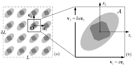
Figure 1: (a) Heterogeneous material – Periodic domain $L$ ; (b) Periodic cell $\mathcal{A}$ and periodicity vectors.

According to the periodicity of the material, $\mathcal{A}$ is the elementary cell period of the elasticity tensor $\mathbb{C}^{(m,\varepsilon)}(\mbox{\boldmath$x$})$:

$$\mathbb{C}^{(m,\varepsilon)}(\mbox{\boldmath$x$}+\mbox{\boldmath$v$}_{i})=\mathbb{C}^{(m,\varepsilon)}(\mbox{\boldmath$x$}),\ \ i=1,2,\ \ \forall\mbox{\boldmath$x$}\in\mathcal{A},$$ (1)

where the superscript $m$ stands for microscopic field. Similarly, the heat conduction tensor $\mbox{\boldmath$K$}^{(m,\varepsilon)}(\mbox{\boldmath$x$})$ and the thermal dilatation tensor $\mbox{\boldmath${\alpha}$}^{(m,\varepsilon)}(\mbox{\boldmath$x$})$ are defined as follows

$$\mbox{\boldmath$K$}^{(m,\varepsilon)}(\mbox{\boldmath$x$}+\mbox{\boldmath$v$}_{i})=\mbox{\boldmath$K$}^{(m,\varepsilon)}(\mbox{\boldmath$x$}),\ \ \mbox{\boldmath${\alpha}$}^{(m,\varepsilon)}(\mbox{\boldmath$x$}+\mbox{\boldmath$v$}_{i})=\mbox{\boldmath${\alpha}$}^{(m,\varepsilon)}(\mbox{\boldmath$x$}),\ \ i=1,2,\ \ \forall\mbox{\boldmath$x$}\in\mathcal{A},$$ (2)

and then the mass diffusion tensor $\mbox{\boldmath$D$}^{(m,\varepsilon)}(\mbox{\boldmath$x$})$ and diffusive expansion tensor $\mbox{\boldmath${\beta}$}^{(m,\varepsilon)}(\mbox{\boldmath$x$})$ become

$$\mbox{\boldmath$D$}^{(m,\varepsilon)}(\mbox{\boldmath$x$}+\mbox{\boldmath$v$}_{i})=\mbox{\boldmath$D$}^{(m,\varepsilon)}(\mbox{\boldmath$x$}),\ \ \mbox{\boldmath${\beta}$}^{(m,\varepsilon)}(\mbox{\boldmath$x$}+\mbox{\boldmath$v$}_{i})=\mbox{\boldmath${\beta}$}^{(m,\varepsilon)}(\mbox{\boldmath$x$}),\ \ i=1,2,\ \ \forall\mbox{\boldmath$x$}\in\mathcal{A}.$$ (3)

The tensors (1), (2) and (3) are commonly referred to as $\mathcal{A}-$periodic functions.

The system is subject to body forces $\mbox{\boldmath$b$}(\mbox{\boldmath$x$})$, heat source $r(\mbox{\boldmath$x$})$ and mass source $s(\mbox{\boldmath$x$})$ which are assumed to be $\mathcal{L}-$periodic with period $\mathcal{L}=[0,L]\times[0,\delta L]$ and to have vanishing mean values on $\mathcal{L}$. Since $L$ is a large multiple of $\varepsilon$, then $\mathcal{L}$ can be assumed to be a representative portion of the overall body. This means that the body forces, heat sources and mass sources are characterized by a period much greater than the microstructural size $\varepsilon$.

Following the procedure reported in Bacigalupo (2014), a non-dimensional unit cell $\mathcal{Q}=[0,1]\times[0,\delta]$ that reproduces the periodic microstructure by rescaling with the small parameter $\varepsilon$ is introduced. Two distinct scales are represented by the macroscopic (slow) variables $\mbox{\boldmath$x$}\in\mathcal{A}$ and the microscopic (fast) variable $\mbox{\boldmath${\xi}$}=\mbox{\boldmath$x$}/\varepsilon\in\mathcal{Q}$ (see for example Bakhvalov and Panasenko (1984); Smyshlyaev and Cherednichenko (2000) and Bacigalupo (2014)). The constitutive tensors (1), (2) and (3) are functions of the microscopic variable, whereas the body forces, heat sources and mass sources depend by the slow macroscopic variable. Consequently, the mapping of both the elasticity and thermodiffusive tensors may be defined on $\mathcal{Q}$ as follows: $\mathbb{C}^{(m,\varepsilon)}(\mbox{\boldmath$x$})=\mathbb{C}^{m}(\mbox{\boldmath${\xi}$}=\mbox{\boldmath$x$}/\varepsilon),\ \mbox{\boldmath$K$}^{(m,\varepsilon)}(\mbox{\boldmath$x$})=\mbox{\boldmath$K$}^{m}(\mbox{\boldmath${\xi}$}=\mbox{\boldmath$x$}/\varepsilon),\ \mbox{\boldmath${\alpha}$}^{(m,\varepsilon)}(\mbox{\boldmath$x$})=\mbox{\boldmath${\alpha}$}^{m}(\mbox{\boldmath${\xi}$}=\mbox{\boldmath$x$}/\varepsilon),\mbox{\boldmath$D$}^{(m,\varepsilon)}(\mbox{\boldmath$x$})=\mbox{\boldmath$D$}^{m}(\mbox{\boldmath${\xi}$}=\mbox{\boldmath$x$}/\varepsilon),\ \mbox{\boldmath${\beta}$}^{(m,\varepsilon)}(\mbox{\boldmath$x$})=\mbox{\boldmath${\beta}$}^{m}(\mbox{\boldmath${\xi}$}=\mbox{\boldmath$x$}/\varepsilon)$, respectively.

The relevant micro-fields are the micro-displacement $\mbox{\boldmath$u$}(\mbox{\boldmath$x$})$, the microscopic temperature $\theta(\mbox{\boldmath$x$})=T(\mbox{\boldmath$x$})-T_{0}$ ($T_{0}$ stands for the temperature of the natural state) and the microscopic chemical potential $\eta(\mbox{\boldmath$x$})$. The micro-stress $\mbox{\boldmath${\sigma}$}(\mbox{\boldmath$x$})$, the microscopic heat and mass fluxes $\mbox{\boldmath$q$}(\mbox{\boldmath$x$})$ and $\mbox{\boldmath$j$}(\mbox{\boldmath$x$})$ are defined by the following constitutive relations:

$$\mbox{\boldmath${\sigma}$}(\mbox{\boldmath$x$})=\mathbb{C}^{m}\left(\frac{\mbox{\boldmath$x$}}{\varepsilon}\right)\mbox{\boldmath${\varepsilon}$}(\mbox{\boldmath$x$})-\mbox{\boldmath${\alpha}$}^{m}\left(\frac{\mbox{\boldmath$x$}}{\varepsilon}\right)\theta(\mbox{\boldmath$x$})-\mbox{\boldmath${\beta}$}^{m}\left(\frac{\mbox{\boldmath$x$}}{\varepsilon}\right)\eta(\mbox{\boldmath$x$}),$$ (4)

$$\mbox{\boldmath$q$}(\mbox{\boldmath$x$})=-\mbox{\boldmath$K$}^{m}\left(\frac{\mbox{\boldmath$x$}}{\varepsilon}\right)\nabla\theta(\mbox{\boldmath$x$}),\quad\mbox{\boldmath$j$}(\mbox{\boldmath$x$})=-\mbox{\boldmath$D$}^{m}\left(\frac{\mbox{\boldmath$x$}}{\varepsilon}\right)\nabla\eta(\mbox{\boldmath$x$}),$$ (5)

where $\mbox{\boldmath${\varepsilon}$}(\mbox{\boldmath$x$})=\mbox{sym}\nabla\mbox{\boldmath$u$}(\mbox{\boldmath$x$})$ is the micro-strain tensor which is assumed to be zero at the fundamental state of the system.

Note that, in eqs. (5) describing the heat and mass fluxes, we confine ourselves to the essential effects and neglect coupling terms, which is an assumption generally accepted in the quasi-static theory of thermodiffusion, see for instance Nowacki (1974).

The micro-stresses (4) and the microscopic fluxes (5) satisfy the local balance equations on the domain $\mathcal{A}$

$$\nabla\cdot\mbox{\boldmath${\sigma}$}(\mbox{\boldmath$x$})+\mbox{\boldmath$b$}(\mbox{\boldmath$x$})=\mbox{\boldmath${0}$},\quad\nabla\cdot\mbox{\boldmath$q$}(\mbox{\boldmath$x$})-r(\mbox{\boldmath$x$})=0,\quad\nabla\cdot\mbox{\boldmath$j$}(\mbox{\boldmath$x$})-s(\mbox{\boldmath$x$})=0.$$ (6)

Substituting expressions (4)-(5) in equations (6) and remembering the symmetry of the elasticity tensor, the resulting set of partial differential equations is written in the form

$$\nabla\cdot\left(\mathbb{C}^{m}\left(\frac{\mbox{\boldmath$x$}}{\varepsilon}\right)\nabla\mbox{\boldmath$u$}(\mbox{\boldmath$x$})\right)-\nabla\cdot\left(\mbox{\boldmath${\alpha}$}^{m}\left(\frac{\mbox{\boldmath$x$}}{\varepsilon}\right)\theta(\mbox{\boldmath$x$})\right)-\nabla\cdot\left(\mbox{\boldmath${\beta}$}^{m}\left(\frac{\mbox{\boldmath$x$}}{\varepsilon}\right)\eta(\mbox{\boldmath$x$})\right)+\mbox{\boldmath$b$}(\mbox{\boldmath$x$})=\mbox{\boldmath${0}$}$$ (7)

$$\nabla\cdot\left(\mbox{\boldmath$K$}^{m}\left(\frac{\mbox{\boldmath$x$}}{\varepsilon}\right)\nabla\theta(\mbox{\boldmath$x$})\right)+r(\mbox{\boldmath$x$})=0,\quad\nabla\cdot\left(\mbox{\boldmath$D$}^{m}\left(\frac{\mbox{\boldmath$x$}}{\varepsilon}\right)\nabla\eta(\mbox{\boldmath$x$})\right)+s(\mbox{\boldmath$x$})=0.$$ (8)

Moreover, at the interface $\Sigma$ between two different phase of the material, the microscopic fields satisfy the following interface conditions:

$$\left.[\mbox{}[\mbox{\boldmath$u$}(\mbox{\boldmath$x$})]\mbox{}]\right|_{\mbox{\boldmath$x$}\in\Sigma}=0,\qquad\left.\left[\mbox{}\left[\left(\mathbb{C}^{m}\left(\frac{\mbox{\boldmath$x$}}{\varepsilon}\right)\nabla\mbox{\boldmath$u$}(\mbox{\boldmath$x$})-\mbox{\boldmath${\alpha}$}^{m}\left(\frac{\mbox{\boldmath$x$}}{\varepsilon}\right)\theta(\mbox{\boldmath$x$})-\mbox{\boldmath${\beta}$}^{m}\left(\frac{\mbox{\boldmath$x$}}{\varepsilon}\right)\eta(\mbox{\boldmath$x$})\right)\mbox{\boldmath$n$}\right]\mbox{}\right]\right|_{\mbox{\boldmath$x$}\in\Sigma}=0,$$ (9)

$$\left.[\mbox{}[\theta(\mbox{\boldmath$x$})]\mbox{}]\right|_{\mbox{\boldmath$x$}\in\Sigma}=0,\qquad\left.\left[\mbox{}\left[\mbox{\boldmath$K$}^{m}\left(\frac{\mbox{\boldmath$x$}}{\varepsilon}\right)\nabla\theta(\mbox{\boldmath$x$})\cdot\mbox{\boldmath$n$}\right]\mbox{}\right]\right|_{\mbox{\boldmath$x$}\in\Sigma}=0,$$ (10)

$$\left.[\mbox{}[\eta(\mbox{\boldmath$x$})]\mbox{}]\right|_{\mbox{\boldmath$x$}\in\Sigma}=0,\qquad\left.\left[\mbox{}\left[\mbox{\boldmath$D$}^{m}\left(\frac{\mbox{\boldmath$x$}}{\varepsilon}\right)\nabla\eta(\mbox{\boldmath$x$})\cdot\mbox{\boldmath$n$}\right]\mbox{}\right]\right|_{\mbox{\boldmath$x$}\in\Sigma}=0,$$ (11)

where the notation $[\mbox{}[f]\mbox{}]=f^{i}(\Sigma)-f^{j}(\Sigma)$ denotes the difference between the values of a function $f$ at the interface $\Sigma$ separating the phase $i$ from the phase $j$.

The micro-displacement, microscopic temperature and chemical potential may be seen in the form $\mbox{\boldmath$u$}(\mbox{\boldmath$x$},\mbox{\boldmath${\xi}$}=\mbox{\boldmath$x$}/\varepsilon),\ \theta(\mbox{\boldmath$x$},\mbox{\boldmath${\xi}$}=\mbox{\boldmath$x$}/\varepsilon),\eta(\mbox{\boldmath$x$},\mbox{\boldmath${\xi}$}=\mbox{\boldmath$x$}/\varepsilon)$ as functions of both the slow and the fast variable.

It is important to note that since $\mbox{\boldmath$u$}(\mbox{\boldmath$x$},\mbox{\boldmath${\xi}$})$, $\theta(\mbox{\boldmath$x$},\mbox{\boldmath${\xi}$})$ and $\theta(\mbox{\boldmath$x$},\mbox{\boldmath${\xi}$})$ are assumed to be $\mathcal{Q}-$periodic smoothing functions with respect to the variable $x$, the interface conditions (9)-(11) can be expressed directly in function of the fast variable ${\xi}$ (Bakhvalov and Panasenko, 1984).

The solution of microscopic field equations (7), (8) is computationally very expensive and provides too detailed results to be of practical use, so that it is convenient to replace the heterogeneous model with an equivalent homogeneous one to obtain equations whose coefficients are not rapidly oscillating while their solutions are close to those of the original equations.

Further in the paper, assuming that the size of the microstructure $\varepsilon$ is sufficiently small with respect to the structural size $L$, an equivalent classical first order thermodiffusive continuum is considered. The overall elastic moduli, thermal and diffusion expansion tensors, thermal and diffusive conduction tensors of a homogeneous continuum equivalent to periodic heterogeneous material reported in Fig. 1 are derived by means of asymptotic homogenization techniques based on the generalization of down-scaling relations. The overall elastic and thermodiffusive properties of the homogeneous continuum are expressed in terms of geometrical, mechanical, thermal and diffusive properties of the microstructure by means of an asymptotic expansion for the microscopic fields. The asymptotic expansion is performed in terms of the parameter $\varepsilon$ that keeps the dependence on the slow variable $x$ separate from the fast one $\mbox{\boldmath${\xi}$}=\mbox{\boldmath$x$}/\varepsilon$ such that two distinct scales are represented.

In the equivalent homogenized continuum, the macro-displacement $\mbox{\boldmath$U$}(\mbox{\boldmath$x$})$ of component $U_{i}$, the macroscopic temperature $\varTheta(\mbox{\boldmath$x$})$ and chemical potential $\varUpsilon(\mbox{\boldmath$x$})$ are defined at a point $x$ in the reference $(\mbox{\boldmath$e$}_{i},\ i=1,2)$. The displacement gradient is given by $\nabla\mbox{\boldmath$U$}(\mbox{\boldmath$x$})=\frac{\partial U_{i}}{\partial x_{j}}\mbox{\boldmath$e$}_{i}\otimes\mbox{\boldmath$e$}_{j}=H_{ij}\mbox{\boldmath$e$}_{i}\otimes\mbox{\boldmath$e$}_{j}=\mbox{\boldmath$H$}(\mbox{\boldmath$x$})$,and then the macroscopic strain is $\mbox{\boldmath$E$}(\mbox{\boldmath$x$})=\mbox{sym}\nabla\mbox{\boldmath$U$}(\mbox{\boldmath$x$})$. The macro-stress $\mbox{\boldmath${\varSigma}$}(\mbox{\boldmath$x$})$ associate to $\mbox{\boldmath$E$}(\mbox{\boldmath$x$})$ are defined as $\mbox{\boldmath${\varSigma}$}(\mbox{\boldmath$x$})=\varSigma_{ij}\mbox{\boldmath$e$}_{i}\otimes\mbox{\boldmath$e$}_{j}$ with $\varSigma_{ij}=\varSigma_{ji}$, and the macroscopic heat and mass fluxes are respectively: $\mbox{\boldmath$Q$}(\mbox{\boldmath$x$})=Q_{i}\mbox{\boldmath$e$}_{i}$ and $\mbox{\boldmath$J$}(\mbox{\boldmath$x$})=J_{i}\mbox{\boldmath$e$}_{i}$.

3 Multiscale analysis and asymptotic solution of the heterogeneous problem

3.1 Down-scaling and up-scaling relations

Following the approaches developed in Bakhvalov and Panasenko (1984); Smyshlyaev and Cherednichenko (2000); Bacigalupo and Gambarotta (2014) and Bacigalupo (2014) for purely elastic problems in periodic heterogeneous media, the microscopic displacement, temperature and chemical potential fields are represented through an asymptotic expansion with respect to the parameter $\varepsilon$, whose terms depend on macroscopic fields and perturbation functions:

$$u_{k}\left(\mbox{\boldmath$x$},\mbox{\boldmath${\xi}$}=\frac{\mbox{\boldmath$x$}}{\varepsilon}\right) =\left[U_{k}(\mbox{\boldmath$x$})+\sum_{l=1}^{+\infty}\varepsilon^{l}\sum_{|q|=l}N_{kpq}^{(l)}(\mbox{\boldmath${\xi}$})\frac{\partial^{l}U_{p}(\mbox{\boldmath$x$})}{\partial x_{q}}+\right.$$

$$\;\;\;\;+\left.\sum_{l=1}^{+\infty}\varepsilon^{l}\sum_{|q|=l-1}\left(\tilde{N}_{kq-1}^{(l)}(\mbox{\boldmath${\xi}$})\frac{\partial^{l-1}\Theta(\mbox{\boldmath$x$})}{\partial x_{q}}+\hat{N}_{kq-1}^{(l)}(\mbox{\boldmath${\xi}$})\frac{\partial^{l-1}\Upsilon(\mbox{\boldmath$x$})}{\partial x_{q}}\right)\right]_{\mbox{\boldmath${\xi}$}=\mbox{\boldmath$x$}/\varepsilon}$$

$$=U_{k}(\mbox{\boldmath$x$})+\varepsilon\left(N_{kpq_{1}}^{(1)}(\mbox{\boldmath${\xi}$})\frac{\partial U_{p}(\mbox{\boldmath$x$})}{\partial x_{q_{1}}}+\tilde{N}_{k}^{(1)}(\mbox{\boldmath${\xi}$})\Theta(\mbox{\boldmath$x$})+\hat{N}_{k}^{(1)}(\mbox{\boldmath${\xi}$})\Upsilon(\mbox{\boldmath$x$})\right)_{\mbox{\boldmath${\xi}$}=\mbox{\boldmath$x$}/\varepsilon}+$$

$$\;\;\;\;+\varepsilon^{2}\left(N_{kpq_{1}q_{2}}^{(2)}(\mbox{\boldmath${\xi}$})\frac{\partial^{2}U_{p}(\mbox{\boldmath$x$})}{\partial x_{q_{1}}\partial x_{q_{2}}}+\tilde{N}_{kq_{1}}^{(2)}(\mbox{\boldmath${\xi}$})\frac{\partial\Theta(\mbox{\boldmath$x$})}{\partial x_{q_{1}}}+\hat{N}_{kq_{1}}^{(2)}(\mbox{\boldmath${\xi}$})\frac{\partial\Upsilon(\mbox{\boldmath$x$})}{\partial x_{q_{1}}}\right)_{\mbox{\boldmath${\xi}$}=\mbox{\boldmath$x$}/\varepsilon}+\cdots,$$

$$\theta\left(\mbox{\boldmath$x$},\mbox{\boldmath${\xi}$}=\frac{\mbox{\boldmath$x$}}{\varepsilon}\right) =\left[\Theta(\mbox{\boldmath$x$})+\sum_{l=1}^{+\infty}\varepsilon^{l}\sum_{|q|=l}\left(M_{q}^{(l)}(\mbox{\boldmath${\xi}$})\frac{\partial^{l}\Theta(\mbox{\boldmath$x$})}{\partial x_{q}}\right)\right]_{\mbox{\boldmath${\xi}$}=\mbox{\boldmath$x$}/\varepsilon}$$

$$=\Theta(\mbox{\boldmath$x$})+\varepsilon\left(M_{q_{1}}^{(1)}(\mbox{\boldmath${\xi}$})\frac{\partial\Theta(\mbox{\boldmath$x$})}{\partial x_{q_{1}}}\right)_{\mbox{\boldmath${\xi}$}=\mbox{\boldmath$x$}/\varepsilon}+\varepsilon^{2}\left(M_{q_{1}q_{2}}^{(2)}(\mbox{\boldmath${\xi}$})\frac{\partial^{2}\Theta(\mbox{\boldmath$x$})}{\partial x_{q_{1}}\partial x_{q_{2}}}\right)_{\mbox{\boldmath${\xi}$}=\mbox{\boldmath$x$}/\varepsilon}+\cdots,$$

$$\eta\left(\mbox{\boldmath$x$},\mbox{\boldmath${\xi}$}=\frac{\mbox{\boldmath$x$}}{\varepsilon}\right) =\left[\Upsilon(\mbox{\boldmath$x$})+\sum_{l=1}^{+\infty}\varepsilon^{l}\sum_{|q|=l}\left(W_{q}^{(l)}(\mbox{\boldmath${\xi}$})\frac{\partial^{l}\Upsilon(\mbox{\boldmath$x$})}{\partial x_{q}}\right)\right]_{\mbox{\boldmath${\xi}$}=\mbox{\boldmath$x$}/\varepsilon}$$

$$=\Upsilon(\mbox{\boldmath$x$})+\varepsilon\left(W_{q_{1}}^{(1)}(\mbox{\boldmath${\xi}$})\frac{\partial\Upsilon(\mbox{\boldmath$x$})}{\partial x_{q_{1}}}\right)_{\mbox{\boldmath${\xi}$}=\mbox{\boldmath$x$}/\varepsilon}+\varepsilon^{2}\left(W_{q_{1}q_{2}}^{(2)}(\mbox{\boldmath${\xi}$})\frac{\partial^{2}\Upsilon(\mbox{\boldmath$x$})}{\partial x_{q_{1}}\partial x_{q_{2}}}\right)_{\mbox{\boldmath${\xi}$}=\mbox{\boldmath$x$}/\varepsilon}+\cdots.$$

In equations (LABEL:Uasym), (LABEL:Tasym) and (LABEL:Easym) (commonly known as down-scaling relations), $q=q_{1},\cdots,q_{l}$ is a multi-index and $\partial^{l}(\cdot)/\partial x_{q}=\partial^{l}(\cdot)/\partial x_{q_{1}}\cdots\partial x_{q_{l}}$. Due to their dependence on the slow space variable $x$, the macroscopic fields $U_{k},\Theta$ and $\Upsilon$ are $\mathcal{L}-$periodic functions. $N_{kpq}^{(l)},M_{q}^{(l)}$ and $W_{q}^{(l)}$ are the mechanical, thermal and diffusive fluctuation functions, respectively, whereas $\tilde{N}_{kq}^{(l)}$ and $\hat{N}_{kq}^{(l)}$ denote the additional fluctuation functions corresponding to the contribution of the thermodiffusion to local displacement. All these perturbation functions depend on the fast space variable $\mbox{\boldmath${\xi}$}=\mbox{\boldmath$x$}/\varepsilon$, and moreover, as it will be shown in Section 3.2, they are $\mathcal{Q}-$periodic. Similarly to the procedure reported in Smyshlyaev and Cherednichenko (2000) and Bacigalupo (2014), the mean value of the fluctuation functions is assumed to vanish on the unit cell $\mathcal{Q}$, this means that the following normalization conditions are satisfied:

$$\left\langle N_{kpq}^{(l)}\right\rangle=\frac{1}{\delta}\int_{\mathcal{Q}}N_{kpq}^{(l)}(\mbox{\boldmath${\xi}$})d\mbox{\boldmath${\xi}$}=0,\quad\left\langle\tilde{N}_{kq}^{(l)}\right\rangle=\frac{1}{\delta}\int_{\mathcal{Q}}\tilde{N}_{kq}^{(l)}(\mbox{\boldmath${\xi}$})d\mbox{\boldmath${\xi}$}=0,\quad\left\langle\hat{N}_{kq}^{(l)}\right\rangle=\frac{1}{\delta}\int_{\mathcal{Q}}\hat{N}_{kq}^{(l)}(\mbox{\boldmath${\xi}$})d\mbox{\boldmath${\xi}$}=0,$$

$$\left\langle M_{q}^{(l)}\right\rangle=\frac{1}{\delta}\int_{\mathcal{Q}}M_{q}^{(l)}(\mbox{\boldmath${\xi}$})d\mbox{\boldmath${\xi}$}=0,\quad\left\langle W_{q}^{(l)}\right\rangle=\frac{1}{\delta}\int_{\mathcal{Q}}W_{q}^{(l)}(\mbox{\boldmath${\xi}$})d\mbox{\boldmath${\xi}$}=0.$$ (15)

Introducing a new variable $\mbox{\boldmath${\zeta}$}\in\mathcal{Q}$ and a vector $\varepsilon\mbox{\boldmath${\zeta}$}\in\mathcal{A}$, which represents the translations of the medium with respect to the $\mathcal{L}-$periodic body forces $\mbox{\boldmath$b$}(\mbox{\boldmath$x$})$, heat sources $r(\mbox{\boldmath$x$})$ and mass sources $s(\mbox{\boldmath$x$})$ (Bacigalupo and Gambarotta, 2014), it can be shown that any $\mathcal{Q}-$periodic function $g(\mbox{\boldmath${\xi}$}+\mbox{\boldmath${\zeta}$})$ satisfies the following invariance property:

$$\left\langle g(\mbox{\boldmath${\xi}$}+\mbox{\boldmath${\zeta}$})\right\rangle=\frac{1}{\delta}\int_{\mathcal{Q}}g(\mbox{\boldmath${\xi}$}+\mbox{\boldmath${\zeta}$})d\mbox{\boldmath${\zeta}$}=\frac{1}{\delta}\int_{\mathcal{Q}}g(\mbox{\boldmath${\xi}$}+\mbox{\boldmath${\zeta}$})d\mbox{\boldmath${\xi}$}.$$ (16)

According to the invariance property (16) and to the normalization conditions (15), the macroscopic fields can be defined as the mean values of the microscopic quantities (LABEL:Uasym), (LABEL:Tasym) and (LABEL:Easym) evaluated on the unit cell $\mathcal{Q}$:

$$U_{k}(\mbox{\boldmath$x$})\doteq\left\langle u_{k}\left(\mbox{\boldmath$x$},\frac{\mbox{\boldmath$x$}}{\varepsilon}+\mbox{\boldmath${\zeta}$}\right)\right\rangle,\quad\Theta(\mbox{\boldmath$x$})\doteq\left\langle\theta\left(\mbox{\boldmath$x$},\frac{\mbox{\boldmath$x$}}{\varepsilon}+\mbox{\boldmath${\zeta}$}\right)\right\rangle,\quad\Upsilon(\mbox{\boldmath$x$})\doteq\left\langle\eta\left(\mbox{\boldmath$x$},\frac{\mbox{\boldmath$x$}}{\varepsilon}+\mbox{\boldmath${\zeta}$}\right)\right\rangle,$$ (17)

Expressions (17) are commonly known as up-scaling relations. More details regarding the structure of the down-scaling relations (LABEL:Uasym), (LABEL:Tasym) and (LABEL:Easym) are provided in Appendix D.

3.2 First-order asymptotic analysis and derivation of the corresponding first-order cell problems

In order to derive exact expressions for the fluctuation functions affecting the behavior of the microscopic fields $u_{k},\theta,\eta$, the down-scaling relations (LABEL:Uasym), (LABEL:Tasym) and (LABEL:Easym) are substituted into the microscopic field equations (7), (8). Remembering the property $\frac{\partial}{\partial x_{j}}f(\boldsymbol{x},\boldsymbol{\xi}=\frac{\boldsymbol{x}}{\varepsilon})=\left(\frac{\partial f}{\partial x_{j}}+\frac{1}{\varepsilon}\frac{\partial f}{\partial\xi_{j}}\right)_{\boldsymbol{\xi}=\boldsymbol{x}/\varepsilon}=\left(\frac{\partial f}{\partial x_{j}}+\frac{f_{,j}}{\varepsilon}\right)_{\boldsymbol{\xi}=\boldsymbol{x}/\varepsilon}$, equation (7) become to the first order approximation

$$\varepsilon^{-1} \biggl{\{}\left[\left(C_{ijkl}^{\varepsilon}N_{kpq_{1},l}^{(1)}\right)_{,j}+C_{ijpq_{1},j}^{\varepsilon}\right]H_{pq_{1}}(\mbox{\boldmath$x$})+\left[\left(C_{ijkl}^{\varepsilon}\tilde{N}_{k,l}^{(1)}\right)_{,j}-\alpha_{ij,j}^{\varepsilon}\right]\Theta(\boldsymbol{x})$$

$$+\left[\left(C_{ijkl}^{\varepsilon}\hat{N}_{k,l}^{(1)}\right)_{,j}-\beta_{ij,j}^{\varepsilon}\right]\Upsilon(\boldsymbol{x})\biggr{\}}+\cdots\cdots+b_{i}(\mbox{\boldmath$x$})=0,\quad\quad i=1,2,$$ (18)

where $H_{pq_{1}}=\partial U_{p}/\partial x_{q_{1}}$ are the components of the macroscopic displacement gradient tensor previously defined. Equations (8) assume the following form

$$\varepsilon^{-1} \biggl{[}\left(K_{ij}^{\varepsilon}M_{q_{1},j}^{(1)}\right)_{,i}+K_{iq_{1},i}^{\varepsilon}\biggr{]}\frac{\partial\Theta}{\partial x_{q_{1}}}+\cdots\cdots+r(\mbox{\boldmath$x$})=0,$$ (19)

$$\varepsilon^{-1} \biggl{[}\left(D_{ik}^{\varepsilon}W_{q_{1},j}^{(1)}\right)_{,i}+D_{iq_{1},i}^{\varepsilon}\biggr{]}\frac{\partial\Upsilon}{\partial x_{q_{1}}}+\cdots\cdots+s(\mbox{\boldmath$x$})=0.$$ (20)

In order to transform the field equation (18), (19) and (20) in a PDEs system with constant coefficients, in which the unknowns are the macroscopic quantities $U_{k}(\mathbf{x})$, $\Theta(\mathbf{x})$ and $\varUpsilon(\mathbf{x})$, the fluctuation functions have to satisfy non-homogeneous equations (first-order cell problems) reported below.

At the order $\varepsilon^{-1}$ from the equation (18) we derive:

$$\left(C_{ijkl}^{\varepsilon}N_{kpq_{1},l}^{(1)}\right)_{,j}+C_{ijpq_{1},j}^{\varepsilon}=n_{ipq_{1}}^{(1)},\quad\left(C_{ijkl}^{\varepsilon}\tilde{N}_{k,l}^{(1)}\right)_{,j}-\alpha_{ij,j}^{\varepsilon}=\tilde{n}_{i}^{(1)},\quad\left(C_{ijkl}^{\varepsilon}\hat{N}_{k,l}^{(1)}\right)_{,j}-\beta_{ij,j}^{\varepsilon}=\hat{n}_{i}^{(1)},$$ (21)

whereas from thermodiffusion equations (19) and (20) we obtain:

$$\left(K_{ij}^{\varepsilon}M_{q_{1},j}^{(1)}\right)_{,i}+K_{iq_{1},i}^{\varepsilon}=m_{q_{1}}^{(1)},\quad\left(D_{ij}^{\varepsilon}W_{q_{1},j}^{(1)}\right)_{,i}+D_{iq_{1},i}^{\varepsilon}=w_{q_{1}}^{(1)},$$ (22)

where:

$$n_{ipq_{1}}^{(1)}=\langle C_{ijpq_{1},j}^{\varepsilon}\rangle=0,\quad\tilde{n}_{i}^{(1)}=-\langle\alpha_{ij,j}^{\varepsilon}\rangle=0,\quad\hat{n}_{i}^{(1)}=-\langle\beta_{ij,j}^{\varepsilon}\rangle=0,$$

$$m_{q_{1}}^{(1)}=\langle K_{iq_{1},i}^{\varepsilon}\rangle=0,\quad w_{q_{1}}^{(1)}=\langle D_{iq_{1},i}^{\varepsilon}\rangle=0.$$ (23)

The properties (23) are consequence of the $\mathcal{Q}-$periodicity of the components $C_{ijpq_{1}}^{\varepsilon},\alpha_{ij}^{\varepsilon},\beta_{ij}^{\varepsilon},K_{iq_{1}}^{\varepsilon}$ and $D_{iq_{1}}^{\varepsilon}$. Note that in equations (18)–(23) the derivatives should be understood in the generalized sense.

The perturbation functions characterizing the down-scaling relations (LABEL:Uasym), (LABEL:Tasym), and (LABEL:Easym) are obtained by the solution of the previously defined cells problems, derived by imposing the normalization conditions (15).

4 Homogenized thermodiffusive Cauchy continuum: field equations and overall properties

The field equations of the first order homogeneous continuum can be obtained by the zero order terms (equations (63) and (64)) of the sequence of PDEs derived applying the asymptotic analysis to the averaged field equation, see Appendix A. This implies that the macroscopic displacement, temperature and chemical potential are approximated as follows:

$$U_{p}(\mathbf{x})\approx U_{p}^{(0)}(\mathbf{x}),\quad\Theta(\mathbf{x})\approx\Theta^{(0)}(\mathbf{x}),\quad\Upsilon(\mathbf{x})\approx\Upsilon^{(0)}(\mathbf{x}).$$ (24)

Alternatively, the field equations of the equivalent Cauchy continuum can be derived considering only the terms of order $\varepsilon^{0}$ in the equations (59), (60) and (61).

The field equations of an homogeneous first order continuum in presence of thermodiffusion are given by

$$C_{iq_{1}pq_{2}}\frac{\partial^{2}U_{p}}{\partial x_{q_{1}}\partial x_{q_{2}}}-\alpha_{iq_{1}}\frac{\partial\Theta}{\partial x_{q_{1}}}-\beta_{iq_{1}}\frac{\partial\Upsilon}{\partial x_{q_{1}}}+b_{i}=0,$$ (25)

$$K_{q_{1}q_{2}}\frac{\partial^{2}\Theta}{\partial x_{q_{1}}\partial x_{q_{2}}}+r=0,\quad D_{q_{1}q_{2}}\frac{\partial^{2}\Upsilon}{\partial x_{q_{1}}\partial x_{q_{2}}}+s=0,$$ (26)

where $C_{iq_{1}pq_{2}}$ are the components of the overall elastic tensor, $\alpha_{iq_{1}}$ and $\beta_{iq_{1}}$ are respectively the components of the overall thermal dilatation and diffusive expansion tensors, $K_{q_{1}q_{2}}$ denotes the components of the overall heat conduction tensor and $D_{q_{1}q_{2}}$ represents the components of the overall mass diffusion tensor. Remembering the approximation (24), the macroscopic field equations (25)–(26) can be compared to the zero order terms of the averaged field equation (63) and (64) for determining the overall properties of the thermodiffusive Cauchy continuum. In order to relate the coefficients $n_{ipq_{1}q_{2}}^{(2)}$, $\tilde{n}_{iq_{1}}^{(2)}$, $\hat{n}_{iq_{1}}^{(2)}$, $m_{q_{1}q_{2}}^{(2)}$, $w_{q_{1}q_{2}}^{(2)}$ contained in the equations (63) and (64) to the overall elastic and thermodiffusive constants of the media $C_{iq_{1}pq_{2}}$, $\alpha_{iq_{1}}$, $\beta_{iq_{1}}$, $K_{q_{1}q_{2}}$, $D_{q_{1}q_{2}}$, the symmetries of the tensors of components $n_{ipq_{1}q_{2}}^{(2)}$, $\tilde{n}_{iq_{1}}^{(2)}$, $\hat{n}_{iq_{1}}^{(2)}$, $m_{q_{1}q_{2}}^{(2)}$, $w_{q_{1}q_{2}}^{(2)}$, and the ellipticity of the field equations (63) and (64) are required. A demonstration of these properties is reported in Appendix C. As a consequence of these properties, it can be observed that: $n_{ipq_{1}q_{2}}^{(2)}=\frac{1}{2}(C_{iq_{1}pq_{2}}+C_{iq_{2}pq_{1}})$, $\tilde{n}_{iq_{1}}^{(2)}=\alpha_{iq_{1}}$, $\hat{n}_{iq_{1}}^{(2)}=\beta_{iq_{1}}$, $m_{q_{1}q_{2}}^{(2)}=K_{q_{1}q_{2}}$ and $w_{q_{1}q_{2}}^{(2)}=D_{q_{1}q_{2}}$. In particular, comparing the field equation (25) to (63), and remembering the relationship between $n_{ipq_{1}q_{2}}^{(2)}$ and $C_{iq_{1}pq_{2}}$, it is easy to note that due to the repetition of the indexes $q_{1}$ and $q_{2}$: $C_{iq_{1}pq_{2}}\frac{\partial^{2}U_{p}}{\partial x_{q_{1}}\partial x_{q_{2}}}=n_{ipq_{1}q_{2}}^{(2)}\frac{\partial^{2}U_{p}}{\partial x_{q_{1}}\partial x_{q_{2}}}=\frac{1}{2}(C_{iq_{1}pq_{2}}+C_{iq_{2}pq_{1}})\frac{\partial^{2}U_{p}}{\partial x_{q_{1}}\partial x_{q_{2}}}$.

The overall elastic and thermodiffusive tensors, obtained in terms of fluctuation functions, and the components of microscopic elastic and thermodiffusive tensors, take the form (see Appendix A for details):

$$C_{iq_{1}pq_{2}}=\frac{1}{4}\left\langle C_{rjkl}^{\varepsilon}\left(N_{riq_{1},j}^{(1)}+\delta_{ri}\delta_{jq_{1}}+N_{rq_{1}i,j}^{(1)}+\delta_{rq_{1}}\delta_{ij}\right)\left(N_{kpq_{2},l}^{(1)}+\delta_{kp}\delta_{q_{2},l}+N_{kq_{2}p,l}^{(1)}+\delta_{kq_{2}}\delta_{lp}\right)\right\rangle$$

$$\alpha_{iq_{1}}=\left\langle C_{iq_{1}kl}^{\varepsilon}\tilde{N}_{k,l}^{(1)}-\alpha_{iq_{1}}^{\varepsilon}\right\rangle,\quad\beta_{iq_{1}}=\left\langle C_{iq_{1}kl}^{\varepsilon}\hat{N}_{k,l}^{(1)}-\beta_{iq_{1}}^{\varepsilon}\right\rangle,$$

$$K_{q_{1}q_{2}}=\left\langle K_{ij}^{\varepsilon}(M_{q_{1},j}^{(1)}+\delta_{jq_{1}})(M_{q_{2},i}^{(1)}+\delta_{iq_{2}})\right\rangle,\quad D_{q_{1}q_{2}}=\left\langle D_{ij}^{\varepsilon}(W_{q_{1},j}^{(1)}+\delta_{jq_{1}})(W_{q_{2},i}^{(1)}+\delta_{iq_{2}})\right\rangle.$$ (27)

The components $C_{iq_{1}pq_{2}}$, $K_{q_{1}q_{2}}$ and $D_{q_{1}q_{2}}$ of the overall constitutive tensors of the material coincide with those derived by asymptotic homogenization techniques applied to uncoupled static elastic (Bakhvalov and Panasenko, 1984; Smyshlyaev and Cherednichenko, 2000; Bacigalupo, 2014) and heat conduction problems (Zhang et al., 2007) in media with periodic microstructures. The components $\alpha_{iq_{1}}$ and $\beta_{iq_{1}}$ of the coupling thermodiffusive tensors have been obtained by means of a consistent generalization of the down-scaling relations (LABEL:Uasym) (LABEL:Tasym) and (LABEL:Easym). These expressions relate the microscopic displacement field to the macroscopic displacements, temperature, chemical potential and their higher order gradients.

5 Illustrative example: homogenization of bi-phase orthotropic layered materials in presence of thermodiffusion

The general results obtained are now applied to the case of a bi-phase layered material in presence of thermodiffusion. Exact analytical expressions for the overall elastic and thermodiffusive constants are derived. Considering a two-dimensional infinite thermodiffusive medium subject to periodic body forces, heat and/or mass sources, the solution obtained applying the proposed homogenized model is compared with the results provided by the analysis of the corresponding heterogeneous problem.

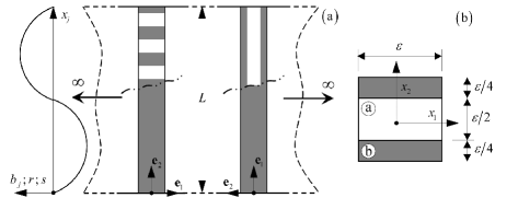
Figure 2: (a) Heterogeneous and homogenized models with $\mathcal{L}$ -periodic body force $b_{j}$, heat sources $r(x_{j})$ and mass sources $s(x_{j})$; (b) Periodic cell and constituents: bi-phase layered material.

5.1 Perturbation functions and overall constitutive constants: exact analytical expressions

Let us consider a layered body obtained as an unbounded $d_{2}-$periodic arrangement of two different layers having thickness $a$ and $b$, where $d_{2}=\varepsilon=a+b$ and $\zeta=a/b$ are defined. The phases are assumed homogeneous and orthotropic, with an orthotropic axis coincident with the layering direction $\mathbf{e}_{1}$, the geometry of the system is shown in Fig. 2. The orthotropic symmetry is assumed for both the elastic and thermodiffusive tensors. The micro-fluctuation functions $N_{riq_{1}}^{(1)}$, $\tilde{N}_{k}^{(1)}$, $\hat{N}_{k}^{(1)}$, $M_{q_{1}}^{(1)}$ and $W_{q_{1}}^{(1)}$ are analytically obtained through the solution of the cell problems formulated in Section 3.2 (see equations (21) and (22) and conditions (23)). Due to the particular properties of symmetry of the microstructure, these functions depend only on the fast variable $\xi_{2}$. This variable is perpendicular to the layering direction $\mathbf{e}_{1}$ (see Fig. 2). The non-vanishing micro-fluctuation functions $N_{riq_{1}}^{(1)}$, $\tilde{N}_{k}^{(1)}$ and $\hat{N}_{k}^{(1)}$, obtained by solving the cell problem of order $\varepsilon^{-1}$ (21) are:

$$N_{211}^{(1)\_a}=\frac{C_{1122}^{b}-C_{1122}^{a}}{C_{2222}^{a}-\zeta C_{2222}^{b}}\xi_{2}^{a};\quad N_{211}^{(1)\_b}=\zeta\frac{C_{1122}^{a}-C_{1122}^{b}}{C_{2222}^{a}-\zeta C_{2222}^{b}}\xi_{2}^{b};$$

$$N_{222}^{(1)\_a}=\frac{C_{2222}^{b}-C_{2222}^{a}}{C_{2222}^{a}-\zeta C_{2222}^{b}}\xi_{2}^{a};\quad N_{211}^{(1)\_b}=\zeta\frac{C_{1122}^{a}-C_{1122}^{b}}{C_{2222}^{a}-\zeta C_{2222}^{b}}\xi_{2}^{b};$$

$$N_{112}^{(1)\_a}=N_{121}^{1\_a}=\frac{C_{1212}^{b}-C_{1212}^{a}}{C_{1212}^{a}-\zeta C_{1212}^{b}}\xi_{2}^{a};\quad N_{112}^{(1)\_b}=N_{121}^{1\_b}=\zeta\frac{C_{1212}^{a}-C_{1212}^{b}}{C_{1212}^{a}-\zeta C_{1212}^{b}}\xi_{2}^{b};$$ (28)

$$\tilde{N}_{2}^{(1)\_a}=-\frac{\alpha_{22}^{b}-\alpha_{22}^{a}}{C_{2222}^{a}+\zeta C_{2222}^{b}}\xi_{2}^{a};\quad\tilde{N}_{2}^{(1)\_b}=\zeta\frac{\alpha_{22}^{b}-\alpha_{22}^{a}}{C_{2222}^{a}+\zeta C_{2222}^{b}}\xi_{2}^{b};$$ (29)

$$\hat{N}_{2}^{(1)\_a}=-\frac{\beta_{22}^{b}-\beta_{22}^{a}}{C_{2222}^{a}+\zeta C_{2222}^{b}}\xi_{2}^{a};\quad\hat{N}_{2}^{(1)\_b}=\zeta\frac{\beta_{22}^{b}-\beta_{22}^{a}}{C_{2222}^{a}+\zeta C_{2222}^{b}}\xi_{2}^{b};$$ (30)

where $\xi_{2}^{a}\in\left[-\frac{\zeta}{2(\zeta+1)},\frac{\zeta}{2(\zeta+1)}\right]$ and $\xi_{2}^{b}\in\left[-\frac{1}{2(\zeta+1)},\frac{1}{2(\zeta+1)}\right]$ are non-dimensional vertical coordinates centered in each layer. The non-vanishing fluctuation functions associate with the thermodiffusion equations, derived by the solution of the cell problems of order $\varepsilon^{-1}$ (22) are:

$$M_{2}^{(1)\_a}=-\frac{K_{22}^{a}-K_{22}^{b}}{K_{22}^{a}-\zeta K_{22}^{b}}\xi_{2}^{a};\quad M_{2}^{(1)\_b}=\zeta\frac{K_{22}^{a}-K_{22}^{b}}{K_{22}^{a}-\zeta K_{22}^{b}}\xi_{2}^{b};$$ (31)

$$W_{2}^{(1)\_a}=-\frac{D_{22}^{a}-D_{22}^{b}}{D_{22}^{a}-\zeta D_{22}^{b}}\xi_{2}^{a};\quad W_{2}^{(1)\_b}=\zeta\frac{D_{22}^{a}-D_{22}^{b}}{D_{22}^{a}-\zeta D_{22}^{b}}\xi_{2}^{b}.$$ (32)

Note that the superscripts ^a,b denote that the elastic and thermodiffusive constants are referred respectively to the phases $a$ and $b$.

In order to derive the overall elastic and thermodiffusive constants corresponding to a first order equivalent continuum, the fluctuation functions (28), (29), (30), (31) and (32) are used into expressions (27). The components of the overall elastic tensor $C_{iq_{1}pq_{2}}$ take the form:

$$C_{1111}=\frac{\zeta^{2}C_{1111}^{a}C_{2222}^{b}+\zeta(C_{1111}^{b}C_{2222}^{b}-(C_{1122}^{a})^{2}+2C_{1122}^{a}C_{1122}^{b}-(C_{1122}^{b})^{2}+C_{1111}^{a}C_{2222}^{a})+C_{1111}^{b}C_{2222}^{a}}{(\zeta+1)(C_{2222}^{a}+\zeta C_{2222}^{b})};$$

$$C_{2222}=\frac{(\zeta+1)C_{2222}^{a}C_{2222}^{b}}{C_{2222}^{a}+\zeta C_{2222}^{b}},\quad C_{1212}=\frac{(\zeta+1)C_{1212}^{a}C_{1212}^{b}}{C_{1212}^{a}+\zeta C_{1212}^{b}},\quad C_{1122}=\frac{C_{1122}^{b}C_{2222}^{a}+\zeta C_{1122}^{a}C_{2222}^{b}}{C_{2222}^{a}+\zeta C_{2222}^{b}}.$$ (33)

The non-vanishing components of the thermal dilatation tensor $\alpha_{iq_{1}}$ and diffusive expansion tensor $\beta_{iq_{1}}$ are respectively given by

$$\alpha_{11}=-\frac{\zeta(C_{1122}^{b}\alpha_{22}^{b}-C_{1122}^{b}\alpha_{22}^{a}-C_{2222}^{b}\alpha_{11}^{b}-C_{1122}^{a}\alpha_{22}^{b}+C_{1122}^{a}\alpha_{22}^{a}-C_{2222}^{a}\alpha_{11}^{a})-\zeta^{2}C_{2222}^{b}\alpha_{11}^{a}-C_{2222}^{a}\alpha_{11}^{b}}{(\zeta+1)(C_{2222}^{a}+\zeta C_{2222}^{b})};$$

$$\alpha_{22}=\frac{\zeta C_{2222}^{b}\alpha_{22}^{a}+\alpha_{22}^{b}C_{2222}^{a}}{C_{2222}^{a}+\zeta C_{2222}^{b}};$$ (34)

$$\beta_{11}=-\frac{\zeta(C_{1122}^{b}\beta_{22}^{b}-C_{1122}^{b}\beta_{22}^{a}-C_{2222}^{b}\beta_{11}^{b}-C_{1122}^{a}\beta_{22}^{b}+C_{1122}^{a}\beta_{22}^{a}-C_{2222}^{a}\beta_{11}^{a})-\zeta^{2}C_{2222}^{b}\beta_{11}^{a}-C_{2222}^{a}\beta_{11}^{b}}{(\zeta+1)(C_{2222}^{a}+\zeta C_{2222}^{b})};$$

$$\beta_{22}=\frac{\zeta C_{2222}^{b}\beta_{22}^{a}+\beta_{22}^{b}C_{2222}^{a}}{C_{2222}^{a}+\zeta C_{2222}^{b}}.$$ (35)

The non-vanishing components of the heat conduction tensor $K_{iq_{1}}$ and mass diffusion tensor $D_{iq_{1}}$ take the form

$$K_{11}=\frac{K_{11}^{b}+\zeta K_{11}^{a}}{\zeta+1},\quad K_{22}=\frac{(\zeta+1)K_{22}^{a}K_{22}^{b}}{K_{22}^{a}+\zeta K_{22}^{b}};$$ (36)

$$D_{11}=\frac{D_{11}^{b}+\zeta D_{11}^{a}}{\zeta+1},\quad D_{22}=\frac{(\zeta+1)D_{22}^{a}D_{22}^{b}}{D_{22}^{a}+\zeta D_{22}^{b}}.$$ (37)

Considering the case of isotropic phases, the components of the elasticity tensor become $C_{1111}^{\varsigma}=C_{2222}^{\varsigma}=\frac{\tilde{E}_{\varsigma}}{1-\tilde{\nu}_{\varsigma}^{2}}$, $C_{1122}^{\varsigma}=\frac{\tilde{\nu}_{\varsigma}\tilde{E}_{\varsigma}}{1-\tilde{\nu}_{\varsigma}^{2}}$, $C_{1212}^{\varsigma}=\frac{\tilde{E}_{\varsigma}}{2(1+\tilde{\nu}_{\varsigma})}$, (with $\varsigma=a,b$), where for plane-strain: $\tilde{E}_{\varsigma}=\frac{E_{\varsigma}}{1-\nu_{\varsigma}^{2}}$, $\tilde{\nu}_{\varsigma}=\frac{\nu_{\varsigma}}{1-\nu_{\varsigma}}$, whereas for plane-stress: $\tilde{E}_{\varsigma}=E_{\varsigma}$, $\tilde{\nu}_{\varsigma}=\nu_{\varsigma}$, being $E_{\varsigma}$ the Young’s modulus and $\nu_{\varsigma}$ the Poisson’s ratio, respectively. The components of the thermal dilatation and diffusive expansion tensors take respectively the forms: $\alpha_{11}^{\varsigma}=\alpha_{22}^{\varsigma}=\alpha^{\varsigma}$, $\beta_{11}^{\varsigma}=\beta_{22}^{\varsigma}=\beta^{\varsigma}$ (note that the coefficients $\alpha^{\varsigma}$ and $\beta^{\varsigma}$ can be expressed in terms of the linear isotropic thermal and diffusive expansion coefficients and the elastic moduli (Nowacki, 1974, 1986). The components of the heat conduction and mass diffusion tensors finally become $K_{11}^{\varsigma}=K_{22}^{\varsigma}=K^{\varsigma}$ and $D_{11}^{\varsigma}=D_{22}^{\varsigma}=D^{\varsigma}$. The overall elastic and thermodiffusive constants for the case of isotropic phases are reported in Appendix C.

By an asymptotic expansion of the constants (33), (34), (35), (36) and (37) in terms of the concentration of the two constituents phases (not reported here for conciseness), it can be easily shown that, if the concentration of the phase $a$ vanishes, the overall elastic and thermodiffusive constants of the bi-phase layered material tend to the values corresponding to phase $b$. Conversely, if the concentration of the phase $a$ tends to one, the same expressions tend to the elastic and thermodiffusive constants of the phase $a$.

In order to simplify the required computations, for the illustrative examples both the phases are assumed to be isotropic, and then the overall elastic and thermodiffusive constants reported in Appendix C are used. These constants can be represented in the non-dimensional form:

$$\tilde{C}_{iq_{1}pq_{2}}(\rho_{C},\zeta,\tilde{\nu}_{a},\tilde{\nu}_{b})=\frac{C_{iq_{1}pq_{2}}}{\hat{C}_{iq_{1}pq_{2}}},\quad\tilde{\alpha}_{iq_{1}}(\rho_{C},\rho_{\alpha},\zeta,\tilde{\nu}_{a},\tilde{\nu}_{b})=\frac{\alpha_{iq_{1}}}{\hat{\alpha}_{iq_{1}}},\quad\tilde{\beta}_{iq_{1}}(\rho_{C},\rho_{\beta},\zeta,\tilde{\nu}_{a},\tilde{\nu}_{b})=\frac{\beta_{iq_{1}}}{\hat{\beta}_{iq_{1}}},$$

$$\tilde{K}_{iq_{1}}(\rho_{K},\zeta)=\frac{K_{iq_{1}}}{\hat{K}_{iq_{1}}},\quad\tilde{D}_{iq_{1}}(\rho_{D},\zeta)=\frac{D_{iq_{1}}}{\hat{D}_{iq_{1}}},$$ (38)

where $\rho_{C}=\tilde{E}_{a}/\tilde{E}_{b},\rho_{\alpha}=\tilde{\alpha}^{a}/\tilde{\alpha}^{b},\rho_{\beta}=\tilde{\beta}^{a}/\tilde{\beta}^{b},\rho_{K}=\tilde{K}^{a}/\tilde{K}^{b},\rho_{D}=\tilde{D}^{a}/\tilde{D}^{b}$, and $\hat{C}_{iq_{1}pq_{2}}=(C_{iq_{1}pq_{2}}^{a}+C_{iq_{1}pq_{2}}^{b})/2,\hat{\alpha}_{iq_{1}}=(\alpha_{iq_{1}}^{a}+\alpha_{iq_{1}}^{b})/2,\hat{\beta}_{iq_{1}}=(\beta_{iq_{1}}^{a}+\beta_{iq_{1}}^{b})/2,\hat{K}_{iq_{1}}=(K_{iq_{1}}^{a}+K_{iq_{1}}^{b})/2,\hat{D}_{iq_{1}}=(D_{iq_{1}}^{a}+D_{iq_{1}}^{b})/2$. It is important to note that if the Poisson’s coefficients of the two phases are identical (i.e. $\nu_{a}=\nu_{b}$), the non-dimensional overall elastic and thermodiffusive constants (38) possess the following property:

$$\tilde{C}_{iq_{1}pq_{2}}(\rho_{C},\zeta,\tilde{\nu})=\tilde{C}_{iq_{1}pq_{2}}(\rho_{C}^{-1},\zeta^{-1},\tilde{\nu}),\quad\tilde{\alpha}_{iq_{1}}(\rho_{C},\rho_{\alpha},\zeta,\tilde{\nu})=\tilde{\alpha}_{iq_{1}}(\rho_{C}^{-1},\rho_{\alpha}^{-1},\zeta^{-1},\tilde{\nu}),$$

$$\tilde{\beta}_{iq_{1}}(\rho_{C},\rho_{\alpha},\zeta,\tilde{\nu})=\tilde{\beta}_{iq_{1}}(\rho_{C}^{-1},\rho_{\alpha}^{-1},\zeta^{-1},\tilde{\nu}),\quad\tilde{K}_{iq_{1}}(\rho_{K},\zeta)=\tilde{K}_{iq_{1}}(\rho_{K}^{-1},\zeta^{-1}),$$

$$\tilde{D}_{iq_{1}}(\rho_{K},\zeta)=\tilde{D}_{iq_{1}}(\rho_{K}^{-1},\zeta^{-1}).$$ (39)

The variation of the normalized components of the overall elasticity tensor $\tilde{C}_{1111}$ and $\tilde{C}_{2222}$ with the ratio $\rho_{C}$ is reported in Figs. 3$/(a)$ and 4$/(a)$, respectively. The same value of the Poisson’s coefficient $\tilde{\nu}=0.3$ has been assumed for both the phases, and several values of the non-dimensional geometrical parameter $\zeta$ has been considered for the computations. It can be observed that for $\rho_{C}=1$, corresponding to the case of two isotropic phases having identical elastic properties, the non-dimensional components of the overall elastic tensor assume the value $\tilde{C}_{iq_{1}pq_{2}}=1$ (i. e. $C_{iq_{1}pq_{2}}=C_{iq_{1}pq_{2}}^{a}=C_{iq_{1}pq_{2}}^{b}$). In Figs. 3$/(b)$ and 4$/(b)$ the components $\tilde{C}_{1111}$ and $\tilde{C}_{2222}$ are plotted as functions of $\zeta$ for different values of $\rho_{C}$ considering the fixed Poisson’s coefficient $\tilde{\nu}=0.3$ identical for both the phases. For $\zeta\rightarrow 0$, the thickness of the phase $a$ vanishes. Consequently, the values of the overall elastic constants tends to those of the phase $b$: $C_{iq_{1}pq_{2}}=C_{iq_{1}pq_{2}}^{b}$, and the limit values assumed by the normalized components of the elastic tensor reported in the figures are $\tilde{C}_{iq_{1}pq_{2}}=2/(1+\rho_{C})$. Conversely, for $\zeta\rightarrow+\infty$ the thickness of the phase $b$ tends to zero, and then $C_{iq_{1}pq_{2}}=C_{iq_{1}pq_{2}}^{a}$ and the non-dimensional constants plotted in Figs. 3$/(b)$-4$/(b)$ assume the limit values $\tilde{C}_{iq_{1}pq_{2}}=2\rho_{C}/(1+\rho_{C}).$ Results (not reported here) show that the normalized components $\tilde{C}_{1212}$ and $\tilde{C}_{1122}$ have a behaviour very similar to that of the component $\tilde{C}_{2222}$.

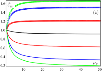
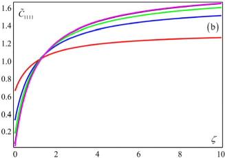
Figure 3: (a) Dimensionless constant $\tilde{C}_{1111}$ vs. the ratio $\rho_{C}$ for $\tilde{\nu}_{a}=\tilde{\nu}_{b}=0.3$ and for different values of the geometric ratio $\zeta$: $\zeta=1/10$ green line, $\zeta=1/5$ blue line, $\zeta=1/2$ red line, $\zeta=1/1$ black line, $\zeta=2$ red points, $\zeta=5$ blue points, $\zeta=10$ green points. (b) Dimensionless constant $\tilde{C}_{1111}$ vs. the geometric ratio $\zeta$ for $\tilde{\nu}_{a}=\tilde{\nu}_{b}=0.3$ and for different values of the ratio $\rho_{C}$: $\rho_{C}=2$ red line, $\rho_{C}=5$ blue line, $\rho_{C}=10$ green line, $\rho_{C}=30$ black line, $\rho_{C}=50$ violet line.

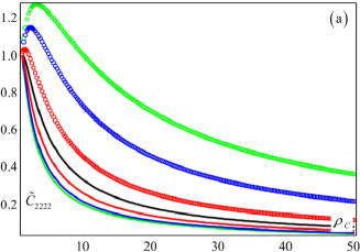
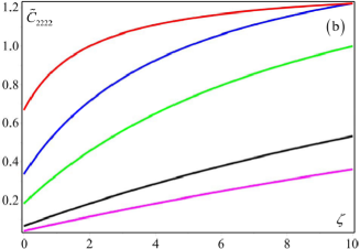
Figure 4: (a) Dimensionless constant $\tilde{C}_{2222}$ vs. the ratio $\rho_{C}$ for $\tilde{\nu}_{a}=\tilde{\nu}_{b}=0.3$ and for different values of the geometric ratio $\zeta$: $\zeta=1/10$ green line, $\zeta=1/5$ blue line, $\zeta=1/2$ red line, $\zeta=1/1$ black line, $\zeta=2$ red points, $\zeta=5$ blue points, $\zeta=10$ green points. (b) Dimensionless constant $\tilde{C}_{2222}$ vs. the geometric ratio $\zeta$ for $\tilde{\nu}_{a}=\tilde{\nu}_{b}=0.3$ and for different values of the ratio $\rho_{C}$: $\rho_{C}=2$ red line, $\rho_{C}=5$ blue line, $\rho_{C}=10$ green line, $\rho_{C}=30$ black line, $\rho_{C}=50$ violet line.

The three-dimensional plots reported in Fig. 5 show the variation of the normalized components of the overall thermal dilatation tensor $\tilde{\alpha}_{11}$ and $\tilde{\alpha}_{22}$ as functions of $\rho_{c}$ and $\rho_{\alpha}$, assuming $\tilde{\nu}=0.3$ for both the phases and $\zeta=1$. In Figs. 6$/(a)$ and 7$/(a)$ the variation of $\tilde{\alpha}_{11}$ and $\tilde{\alpha}_{22}$ with the non-dimensional ratio $\rho_{C}$ is reported for several values of $\zeta$ assuming $\tilde{\nu}_{a}=\tilde{\nu}_{b}=\tilde{\nu}=0.3$ and $\rho_{\alpha}=2$. For $\rho_{C}=1$, corresponding to the case of two isotropic phases with identical elastic constants but different thermal dilatation properties, the normalized components of the overall thermal dilatation tensor tend to the values $\tilde{\alpha}_{iq_{1}}=2(\zeta\rho_{\alpha}+1)/[(\rho_{\alpha}+1)(\zeta+1)]$ (i.e. $\alpha_{iq_{1}}=(\alpha_{iq_{1}}^{a}\zeta+\alpha_{iq_{1}}^{b})/(\zeta+1)$). In the case where $\rho_{C}=1$ and also $\rho_{\alpha}=1$, both the elastic and thermal dilatation tensors of the two phases are identical, and then $\tilde{\alpha}_{iq_{1}}=1$. In Figs. 6$/(b)$ and 7$/(b)$ the same constants $\hat{\alpha}_{11}$ and $\hat{\alpha}_{22}$ are plotted as functions of $\zeta$ for $\tilde{\nu}=0.3$, $\rho_{\alpha}=2$ and several different values of $\rho_{C}$. For $\zeta\rightarrow 0$, the thickness for the phase $a$ vanishes, and the elements of the overall thermal dilatation tensor tends to those of the phase $b$ (i.e. $\alpha_{iq_{1}}=\alpha_{iq_{1}}^{b}$). As it can be observed in the figures, in this case the normalized constants tend to a limit value which is the same for any value of $\rho_{C}$ (i.e. $\tilde{\alpha}_{iq_{1}}=2/(1+\rho_{\alpha})$). This value can be easily derived by using expressions for $\alpha_{11}$ and $\alpha_{22}$ reported in Appendix C. Conversely, for $\zeta\rightarrow+\infty$, the thickness of the layer $b$ tends to zero, the effective thermal dilatation constants tend to those of the phase $a$ (i.e. $\alpha_{iq_{1}}=\alpha_{iq_{1}}^{a}$) and the normalized components $\tilde{\alpha}_{11}$ and $\tilde{\alpha}_{22}$ reported in Figs. 6$/(b)$ and 7$/(b)$ assume the values $\tilde{\alpha}_{iq_{1}}=2\rho_{\alpha}/(1+\rho_{\alpha})$. The properties of the normalized elements of the overall diffusive expansion tensor $\tilde{\beta}_{11}$ and $\tilde{\beta}_{22}$ are similar to those of $\tilde{\alpha}_{11}$ and $\tilde{\alpha}_{22}$, and can be easily studied substituting the non-dimensional ratio $\rho_{\alpha}$ with $\rho_{\beta}$.

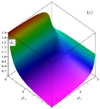
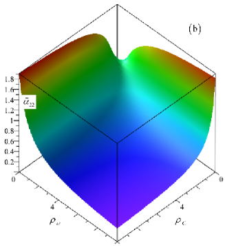
Figure 5: Dimensionless component $\tilde{\alpha}_{11}$ (a), $\tilde{\alpha}_{22}$ (b) vs. the ratios $\rho_{C}$ and $\rho_{\alpha}$ for $\tilde{\nu}_{a}=\tilde{\nu}_{b}=0.3$ and $\zeta=1/2$.

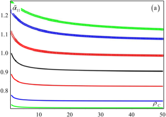
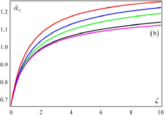
Figure 6: Dimensionless component $\tilde{\alpha}_{11}$ vs. the ratio $\rho_{C}$ for $\tilde{\nu}_{a}=\tilde{\nu}_{b}=0.3$, $\rho_{\alpha}=2$ and for different values of the geometric ratio $\zeta$: $\zeta=1/10$ green line, $\zeta=1/5$ blue line, $\zeta=1/2$ red line, $\zeta=1/1$ black line, $\zeta=2$ red points, $\zeta=5$ blue points, $\zeta=10$ green points. (b) Dimensionless component $\alpha_{11}$ vs. the ratio $\rho_{C}$ for $\tilde{\nu}_{a}=\tilde{\nu}_{b}=0.3$, $\rho_{\alpha}=2$ and for different values of the geometric ratio $\rho_{C}$: $\rho_{C}=2$ red line, $\rho_{C}=5$ blue line, $\rho_{C}=10$ green line, $\rho_{C}=30$ black line, $\rho_{C}=50$ violet line.

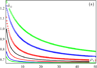
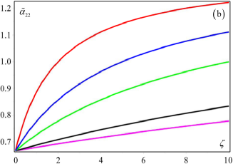
Figure 7: Dimensionless component $\tilde{\alpha}_{22}$ vs. the ratio $\rho_{C}$ for $\tilde{\nu}_{a}=\tilde{\nu}_{b}=0.3$, $\rho_{\alpha}=2$ and for different values of the geometric ratio $\zeta$: $\zeta=1/10$ green line, $\zeta=1/5$ blue line, $\zeta=1/2$ red line, $\zeta=1/1$ black line, $\zeta=2$ red points, $\zeta=5$ blue points, $\zeta=10$ green points. (b) Dimensionless component $\alpha_{22}$ vs. the ratio $\rho_{C}$ for $\tilde{\nu}_{a}=\tilde{\nu}_{b}=0.3$, $\rho_{\alpha}=2$ and for different values of the geometric ratio $\rho_{C}$: $\rho_{C}=2$ red line, $\rho_{C}=5$ blue line, $\rho_{C}=10$ green line, $\rho_{C}=30$ black line, $\rho_{C}=50$ violet line.

The variation of the normalized components of the overall heat conduction tensor $\tilde{K}_{11}$ and $\tilde{K}_{22}$ with the non-dimensional ratio $\rho_{K}$ are shown in Figs. 8$/(a)$ and 9$/(a)$. Several values of $\zeta$ have been assumed for the computations. It can be observed that for $\rho_{K}=1$, we have $\tilde{K}_{iq_{1}}=1$. This is due to the fact that the value $\rho_{K}=1$ corresponds to the case where the heat conduction of the two phases are identical, and then $K_{iq_{1}}^{a}=K_{iq_{1}}^{b}$. In Figs. 8$/(a)$ and 9$/(b)$ the same non-dimensional components $\tilde{K}_{11}$ and $\tilde{K}_{22}$ are reported as functions of $\zeta$ for different values of $\rho_{K}$. As it is shown by these figures, for $\zeta\rightarrow 0$, $\tilde{K}_{11}$ and $\tilde{K}_{22}$ tends to a finite value depending on $\rho_{K}$. This limit correspond to the case of vanishing thickness of the layer $a$, where $K_{iq_{1}}=K_{iq_{1}}^{b}$, and then $\tilde{K}_{iq_{1}}=2/(1+\rho_{K})$. In the limit $\zeta\rightarrow+\infty$, for which the thickness of the layer $b$ vanishes and $K_{iq_{1}}=K_{iq_{1}}^{a}$, the normalized components of the overall heat conductivity tensor tend to a finite value given by $\tilde{K}_{iq_{1}}=2\rho_{K}/(1+\rho_{K})$. The non-dimensional components of the overall mass diffusion tensor $\tilde{D}_{11}$ and $\tilde{D}_{22}$ are characterized by properties similar to those of $\tilde{K}_{11}$ and $\tilde{K}_{22}$, and can be studied substituting the non-dimensional ratio $\rho_{K}$ with $\rho_{D}$.

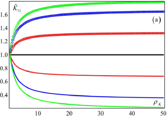
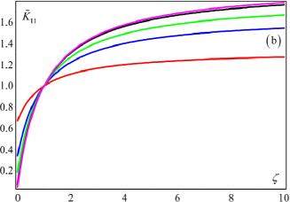
Figure 8: Dimensionless component $\tilde{K}_{11}$ vs. the ratio $\rho_{K}$ for different values of the geometric ratio $\zeta$: $\zeta=1/10$ green line, $\zeta=1/5$ blue line, $\zeta=1/2$ red line, $\zeta=1/1$ black line, $\zeta=2$ red points, $\zeta=5$ blue points, $\zeta=10$ green points. (b) Dimensionless component $\tilde{K}_{11}$ vs. the ratio $\rho_{K}$ for different values of the ratio $\rho_{K}$: $\rho_{K}=2$ red line, $\rho_{K}=5$ blue line, $\rho_{K}=10$ green line, $\rho_{K}=30$ black line, $\rho_{K}=50$ violet line.

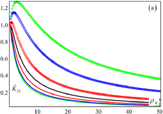
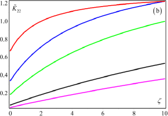
Figure 9: Dimensionless component $\tilde{K}_{22}$ vs. the ratio $\rho_{K}$ for different values of the geometric ratio $\zeta$: $\zeta=1/10$ green line, $\zeta=1/5$ blue line, $\zeta=1/2$ red line, $\zeta=1/1$ black line, $\zeta=2$ red points, $\zeta=5$ blue points, $\zeta=10$ green points. (b) Dimensionless component $\tilde{K}_{22}$ vs. the ratio $\rho_{K}$ for different values of the ratio $\rho_{K}$: $\rho_{K}=2$ red line, $\rho_{K}=5$ blue line, $\rho_{K}=10$ green line, $\rho_{K}=30$ black line, $\rho_{K}=50$ violet line.

5.2 Comparative analysis: homogenized model vs heterogeneous material

In order to study the capabilities of the proposed homogenization procedure, the two-dimensional bi-phase orthotropic layered material shown in Fig. 2 is assumed to be subjected to $\mathcal{L}$-periodic harmonic body forces $b_{i}$, directed along the orthotropy direction $x_{j}$ (see Fig. 2) and $\mathcal{L}$-periodic heat and mass sources $r(x_{j})$ and $s(x_{j})$:

$$b_{j}(x_{j})=B_{j}e^{i\cfrac{2\pi mx_{j}}{L_{j}}},\quad r(x_{j})=Re^{i\cfrac{2\pi nx_{j}}{L_{j}}},\quad s(x_{j})=Se^{i\cfrac{2\pi px_{j}}{L_{j}}},$$ (40)

where: $j=1,2$; $L_{1}=L_{2}=L$; $B_{i},R,S\in\mathbb{C}$; $m,n,p\in\mathbb{Z}$; and $i^{2}=-1$.

This problem is analyzed by applying the homogenized first-order model with overall elastic and thermodiffusive constants derived from the homogenization of the periodic cell through the approach developed in previous Sections. The obtained results are then compared with those derived by means of a fully heterogeneous modelling procedure. Due to the periodicity of the heterogeneous material, body forces, heat and mass sources considered, only an horizontal (or vertical) characteristic portion of length $L$ of the heterogeneous model is analyzed (Fig. 2b). In order to assess the reliability of the homogenized model, the macroscopic displacement, temperature and chemical potential fields are compared to the corresponding fields in the heterogeneous model by means of the up-scaling relations (17).

The overall elastic and thermodiffusive constants involving the fluctuation functions are obtained in exact analytical forms via expressions (33), (34), (35), (37), and (36). Conversely, the solution of the heterogeneous problem with $\mathcal{L}-$periodic harmonic body forces is computed via FE analysis with periodic boundary conditions on the displacement temperature and chemical potential fields. For the considered two-dimensional body subject to body forces along the orthotropy axes, heat and mass sources, the homogenized field equations (25)–(26) take the form:

$$C_{jjjj}\frac{\partial^{2}U_{j}}{\partial x_{j}^{2}}-\alpha_{jj}\frac{\partial\Theta}{\partial x_{j}}-\beta_{jj}\frac{\partial\Upsilon}{\partial x_{j}}+b_{j}=0,\quad K_{jj}\frac{\partial^{2}\Theta}{\partial x_{j}^{2}}+r=0,\quad D_{jj}\frac{\partial^{2}\Upsilon}{\partial x_{j}^{2}}+s=0,$$ (41)

where $j=1,2$ are not summed indexes. Equations (41) describe an extensional problem in presence of thermodiffusion. Considering body forces, heat and mass sources of the form (40), the macroscopic displacements, temperature and chemical potential fields are given by

$$U_{j}(x_{j})=\frac{B_{j}L^{2}}{C_{jjjj}(2\pi m)^{2}}e^{i\frac{2\pi mx_{j}}{L_{j}}}-i\left[\frac{R\alpha_{jj}L^{3}}{C_{jjjj}K_{jj}(2\pi n)^{3}}e^{i\frac{2\pi nx_{j}}{L_{j}}}+\frac{S\beta_{jj}L^{3}}{C_{jjjj}D_{jj}(2\pi p)^{3}}e^{i\frac{2\pi px_{j}}{L_{j}}}\right],$$ (42)

$$\Theta(x_{j})=\frac{RL^{2}}{K_{jj}(2\pi n)^{2}}e^{i\frac{2\pi nx_{j}}{L_{j}}},\quad\Upsilon(x_{j})=\frac{SL^{2}}{D_{jj}(2\pi p)^{2}}e^{i\frac{2\pi px_{j}}{L_{j}}},$$ (43)

where $j=1,2$ are still not summed indexes. In order to compare the behavior of the derived analytical solution with the numerical results provided by the heterogeneous model, only the real part of macroscopic fields (42), (43) is accounted. Moreover, the imaginary part of the amplitudes $B_{j}$, $R$ and $S$ is assumed to be zero. The real part of expressions (42), (43) can be written in the non-dimensional form:

$$U_{j}^{*}(x_{j})=\cos\left(\frac{2\pi mx_{j}}{L_{j}}\right)+\varXi_{jj}^{\alpha}\frac{m^{2}}{2\pi n^{3}}\sin\left(\frac{2\pi nx_{j}}{L_{j}}\right)+\varXi_{jj}^{\beta}\frac{m^{2}}{2\pi p^{3}}\sin\left(\frac{2\pi px_{j}}{L_{j}}\right),$$ (44)

$$\Theta^{*}(x_{j})=\cos\left(\frac{2\pi nx_{j}}{L_{j}}\right),\quad\Upsilon^{*}(x_{j})=\cos\left(\frac{2\pi px_{j}}{L_{j}}\right),$$ (45)

where $U_{j}^{*}=\frac{U_{j}C_{jjjj}(2\pi m)^{2}}{B_{j}L_{j}^{2}}$, $\Theta^{*}=\frac{\Theta K_{jj}(2\pi n)^{2}}{RL_{j}^{2}}$, $\Upsilon^{*}=\frac{\Upsilon D_{jj}(2\pi p)^{2}}{SL_{j}^{2}}$; and $\varXi_{jj}^{\alpha}=\frac{\alpha_{jj}RL_{j}}{K_{jj}B_{j}}$ and $\varXi_{jj}^{\beta}=\frac{\beta_{jj}SL_{j}}{D_{jj}B_{j}}$, $j=1,2$ are still not summed indexes.

The amplitude functions $\varXi_{jj}^{\alpha}$ and $\varXi_{jj}^{\beta}$ are associated respectively with the thermal expansion and mass diffusion contribution to the macroscopic displacement (44) along the direction $\mathbf{e}_{j}$. In order to study the influence of the geometrical, elastic and thermodiffusive properties of the phases on $\varXi_{jj}^{\alpha}$ and $\varXi_{jj}^{\beta}$, the following non-dimensional form for these functions is introduced:

$$\tilde{\varXi}_{jj}^{\alpha}(\rho_{C},\rho_{\alpha},\rho_{K},\zeta,\tilde{\nu}_{a},\tilde{\nu}_{b})=\frac{\varXi_{jj}^{\alpha}}{\hat{\varXi}_{jj}^{\alpha}},\quad\tilde{\varXi}_{jj}^{\beta}(\rho_{C},\rho_{\beta},\rho_{K},\zeta,\tilde{\nu}_{a},\tilde{\nu}_{b})=\frac{\varXi_{jj}^{\beta}}{\hat{\varXi}_{jj}^{\beta}},\quad\mbox{with}\ j=1,2,$$ (46)

where $\hat{\varXi}_{jj}^{\alpha}=RL_{j}(\alpha^{a}+\alpha^{b})/B_{j}(K^{a}+K^{b})$ and $\hat{\varXi}_{jj}^{\beta}=RL_{j}(\beta^{a}+\beta^{b})/B_{j}(D^{a}+D^{b})$. In the case where the two phases possess the same value of the Poisson’s coefficient ($\tilde{\nu}_{a}=\tilde{\nu}_{b}$), the following property is verified for the normalized amplitude functions:

$$\tilde{\varXi}_{jj}^{\alpha}(\rho_{C},\rho_{\alpha},\rho_{K},\zeta,\tilde{\nu})=\tilde{\varXi}_{jj}^{\alpha}(\rho_{C}^{-1},\rho_{\alpha}^{-1},\rho_{K}^{-1},\tilde{\nu}),\quad\tilde{\varXi}_{jj}^{\alpha}(\rho_{C},\rho_{\beta},\rho_{K},\zeta,\tilde{\nu})=\tilde{\varXi}_{jj}^{\beta}(\rho_{C}^{-1},\rho_{\alpha}^{-1},\rho_{K}^{-1},\tilde{\nu}).$$ (47)

The three-dimensional plot reported in Fig. 10$/(a)$ shows the variation of the normalized amplitude component $\tilde{\varXi}_{11}^{\alpha}$ with $\rho_{\alpha}$ and $\rho_{K}$ for $\tilde{\nu}_{a}=\tilde{\nu}_{b}=0.3$, $\rho_{C}=10$ and $\zeta=1$. In Fig. 10$/(b)$ the same component $\tilde{\varXi}_{11}^{\alpha}$, which represents the contribution of the thermal expansion to the macroscopic displacement along the direction $\mathbf{e}_{1}$, is plotted as a function of $\rho_{C}$ assuming $\tilde{\nu}_{a}=\tilde{\nu}_{b}=0.3$, $\rho_{\alpha}=\rho_{K}=10$ and several values of the dimensionless ratio $\zeta$. The variation of the normalized component $\tilde{\varXi}_{22}^{\alpha}$, corresponding to the contribution of the thermal expansion to the macroscopic displacement along $\mathbf{e}_{2}$ (see Fig. 2), is reported in Fig. 11$/(a)$ as a function of $\rho_{\alpha}$ and $\rho_{K}$ for $\tilde{\nu}_{a}=\tilde{\nu}_{b}=0.3$, $\rho_{C}=10$ and $\zeta=1$, and in Fig. 11$/(b)$ as a function of $\rho_{C}$ assuming $\tilde{\nu}_{a}=\tilde{\nu}_{b}=0.3$, $\rho_{\alpha}=\rho_{K}=10$. Observing the curves reported in the figures, it can be noted that the normalized amplitude $\tilde{\varXi}_{22}^{\alpha}$, associate to the component of the macroscopic displacement $U^{*}_{2}(x_{2})$ parallel to the stratification direction, is greater than the amplitude $\tilde{\varXi}_{11}^{\alpha}$ which correspond to the component $U^{*}_{1}(x_{1})$ parallel to the stratification direction. The dimensionless amplitude $\tilde{\varXi}_{11}^{\beta}$ and $\tilde{\varXi}_{22}^{\beta}$, associated to the contributions of the mass diffusion respectively to $U^{*}_{1}(x_{1})$ and $U^{*}_{2}(x_{2})$, are characterized by the same properties of $\tilde{\varXi}_{11}^{\alpha}$ and $\tilde{\varXi}_{22}^{\alpha}$, and their behavior can be easily studied substituting the non-dimensional ratios $\rho_{\alpha}$ and $\rho_{K}$ with $\rho_{\beta}$ and $\rho_{D}$.

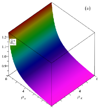
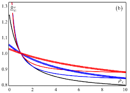
Figure 10: (a) Dimensionless amplitude $\tilde{\Xi}{}_{11}^{\alpha}$ vs. the ratios $\rho_{\alpha}$ and $\rho_{K}$ for $\tilde{\nu}_{a}=\tilde{\nu}_{b}=0.3$, $\rho_{C}$=10 and $\zeta=1$. (b) Dimensionless amplitude $\tilde{\Xi}{}_{jj}^{\alpha}$ vs. the ratios $\rho_{C}$ for $\tilde{\nu}_{a}=\tilde{\nu}_{b}=0.3$, $\rho_{\alpha}=\rho_{K}=10$ and $\zeta=1$ for different values of the geometric ratio $\zeta$: $\zeta=1/10$ red line, $\zeta=1/5$ blue line, $\zeta=1$ black line, $\zeta=5$ blue line points, $\zeta=10$ red line points.

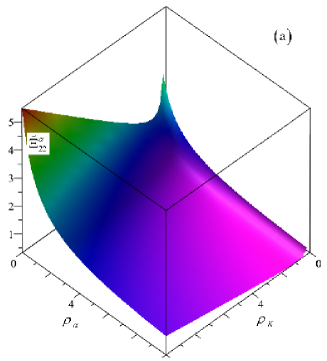
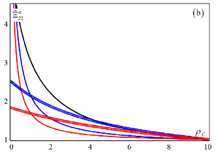
Figure 11: (a) Dimensionless amplitude $\tilde{\Xi}{}_{22}^{\alpha}$ vs. the ratios $\rho_{\alpha}$ and $\rho_{K}$ for $\tilde{\nu}_{a}=\tilde{\nu}_{b}=0.3$, $\rho_{C}$=10 and $\zeta=1$. (b) Dimensionless amplitude $\tilde{\Xi}{}_{22}^{\alpha}$ vs. the ratios $\rho_{C}$ for $\tilde{\nu}_{a}=\tilde{\nu}_{b}=0.3$, $\rho_{\alpha}=\rho_{K}=10$ and $\zeta=1$ for different values of the geometric ratio $\zeta$: $\zeta=1/10$ red line, $\zeta=1/5$ blue line, $\zeta=1$ black line, $\zeta=5$ blue line points, $\zeta=10$ red line points.

The analytical solution (44) and (45), derived by the solution of the homogenized field equations (41) is now compared with the results obtained by the finite element analysis of the heterogeneous problem corresponding to the bi-phase layered material reported in Fig. 2 subject to harmonic body forces, heat and mass sources. More precisely, finite element analysis of the heterogeneous problem, performed by means of the program COMSOL Multiphysics, provides the local fields $u_{j}$, $\theta$, $\eta$ which are used together with the up-scaling relations (17) for obtaining the macro-scopic fields $U_{j}$, $\Theta$ and $\Upsilon$. These macro-scopic quantities are compared with the analytical expressions (44) and (45). Plane stress condition has been assumed for both the solution of the homogenized equations and the heterogeneous problem, and two isotropic phases with the same value of the Poisson’s coefficient $\nu_{a}=\nu_{b}=0.3$ have been considered.

In Fig. 12, the macroscopic displacement component $U_{1}^{*}$ and temperature $\Theta^{*}$ evaluated using analytical expressions (44) and (45)₁ are reported as functions of the normalized spatial coordinate $x_{1}/L$ (continuous lines in the figure) and compared with the numerical results obtained by the heterogeneous model assuming periodic body forces $b_{1}(x_{1})$ and heat sources $r(x_{1})$ and considering the value of the amplitude $\tilde{\varXi}_{11}^{\alpha}=1$ (diamonds in the figure). The following values for the geometrical parameters, the ratios between the elastic and of thermodiffusive constants have been assumed: $L/\varepsilon=10$, $\rho_{C}=10$, $\rho_{\alpha}=10$, $\rho_{\beta}=0$ $\rho_{K}=10$, $\rho_{D}=0$, the effects of the mass diffusion have been neglected in this example. The macroscopic displacement and temperature fields are plotted for the characteristic portion of length $L_{1}=L$, corresponding to $x_{1}/L=1$ (i. e. for $0\leq x_{1}/L\leq 1$), and several values for the wave numbers $m,n\in\mathbb{Z}$ have been considered. Observing the curves, for both the quantities $U_{1}^{*}(x_{1}/L)$ and $\Theta^{*}(x_{1}/L)$ a good agreement is detected between the results derived by means of the first order homogenization approach and those obtained by the heterogeneous model.

Results for the macroscopic displacement component $U^{*}_{2}$ and temperature in $\Theta^{*}$ along the characteristic portion of length $L_{2}=L$ in direction parallel to $\mathbf{e}_{2}$ (not reported here for conciseness) show a good agreement between the solution obtained by means of the first-order asymptotic homogenization method and the values obtained by means of finite element analysis of the heterogeneous problem.

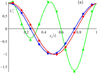
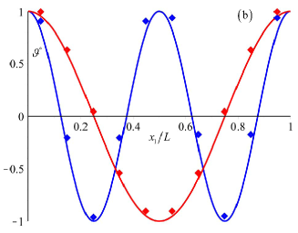
Figure 12: Macroscopic displacement component $U_{1}^{*}$ and temperature fields $\Theta^{*}$ due to harmonic body force $b_{1}$ and temperature source $r$. The heterogeneous model (diamonds) is compared with the homogenized first order model. (a) Dimensionless macro displacement $U_{1}^{*}$ vs. the ratio $x_{1}/L$ for $\Xi_{11}^{\alpha}=1$ for different values of wave number $n$, $m$ ($n=1$, $m=1$ red line; $n=2$, $m=1$ blue line; $n=1$, $m=2$ green line). (b) Macro temperature $\Theta^{*}$ vs. the ratio $x_{1}/L$ for different values of wave number $n$ ($n=1$ red line; $n=2$, blue line).

In Fig. 13, the variation of the normalized component of the macroscopic displacement $U^{*}_{1}(x_{1}/L)$, temperature $\Theta^{*}(x_{1}/L)$ and chemical potential $\Upsilon^{*}(x_{1}/L)$ along the characteristic portion of length $L_{1}=L$ is plotted as a function of $x_{1}/L$. Two isotropic phases having the same Poisson’s coefficient $\nu=0.3$ have been assumed, and the same values of the previous example have been assigned to the geometrical, elastic and thermal parameters. The amplitude of the mass diffusion contribution to the displacement is assumed to be $\tilde{\varXi}_{11}^{\beta}=1$, and $\rho_{K}=10$. Similarly to the previous case, for the finite element analysis of the heterogeneous elastic thermodiffusive problem harmonic body forces $b_{1}(x_{1})$, heat and mass sources $r(x_{1})$ and $s(x_{1})$ have been introduced. The reported curves show a good agreement between the results obtained by the asymptotic homogenization (continuous lines the figure) and those provided by the heterogeneous elastic thermodiffusive model (diamonds in the figure). The good agreement between the results coming from the two different approaches can be observed for $U^{*}_{1}(x_{1}/L)$ in Fig. 13$/{(a),(b)}$, for $\Theta^{*}(x_{1}/L)$ in Fig. 13$/{(b)}$ and for $\Upsilon^{*}(x_{1}/L)$ in Fig. 13$/{(d)}$. Similar results are obtained for the macroscopic displacement $U^{*}_{2}$, temperature $\Theta^{*}$ and chemical potential $\Upsilon^{*}$ along the characteristic portion of length $L_{2}=L$ in direction parallel to $\mathbf{e}_{2}$

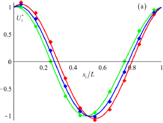
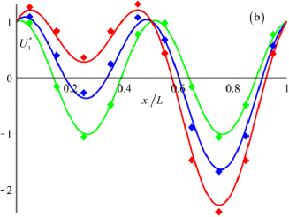
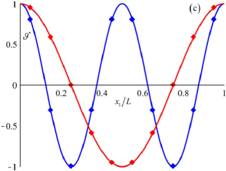
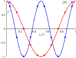
Figure 13: Macroscopic displacement component $U_{1}^{*}$, temperature $\Theta^{*}$, and chemical potential $\varUpsilon^{*}$ due to harmonic body force $b_{1}$ and temperature and mass sources $r$,$s$ respectively. The heterogeneous model (diamonds) is compared with the homogenized first order model. Dimensionless macro displacement $U_{1}^{*}$ vs. the ratio $x_{1}/L$ for $\Xi_{11}^{\alpha}=1$,$\Xi_{11}^{\beta}=1$ and wave number $m=1$ (a), $m=2$ (b) for different values of wave number $n$, $p$ ($n=1$, $p=1$ red line; $n=2$, $p=1$ blue line; $n=2$, $p=2$ green line). (c) Macro temperature $\Theta^{*}$ vs. the ratio $x_{1}/L$ for different values of wave number $n$ ($n=1$ red line; $n=2$, blue line). (d) Macro concentration $\varUpsilon^{*}$ vs. the ratio $x_{1}/L$ for different values of wave number $p$ ($p=1$ red line; $p=2$, blue line).

6 Conclusions

A general asymptotic homogenization approach for describing the static elastic, thermal and diffusive properties of periodic composite materials in presence of thermodiffusion is proposed. Down-scaling relations associating the displacements, temperature and chemical potential at the micro-scale to the corresponding fields at the macro-scale are introduced. Perturbation functions are defined for representing the effects of the microstructures on the microscopic displacement, temperature, chemical potential and on the coupling effects between these fields. These perturbation functions are obtained through the solution of non-homogeneous problems on the cell defining periodic boundary conditions and normalization conditions (up-scaling relations).

Averaged field equations of infinite order are derived for the considered class of periodic thermodiffusive materials, and an original formal solution is performed by means of power series expansion of the macroscopic displacements, temperature and chemical potential fields. Field equation for the homogenized Cauchy thermodiffusive continuum are derived, and exact expressions for the overall elastic and thermodiffusive constants of this equivalent first order medium are obtained.

An example of application of the developed general method to the illustrative case of a two-dimensional bi-phase orthotropic layered material is provided. The effective elastic and thermodiffusive constants of this particular composite material are determined using the general expressions derived by the asymptotic homogenization procedure. Analytical expressions for the macroscopic fields derived by the solution of the homogenized equations corresponding to the first order equivalent continuum. Finite element analysis of the corresponding heterogeneous model is performed assuming periodic body forces, heat and mass sources acting on the considered bi-phase layered composite. In order to compare the analytical solution of the homogenized equations with the numerical results obtained by the heterogeneous model, the microscopic fields computed by finite elements techniques are used to estimate the macroscopic displacements, temperature and chemical potential fields by means of the up-scaling relations defined in the paper. The good agreement detected between the solution derived by the homogenized first order equations and the numerical results obtained by the heterogeneous model through the up-scaling relations represents an important validation of the accuracy of the proposed asymptotic homogenization approach.

Thanks to the great versatility of the asymptotic homogenization techniques and to the proposed general rigorous formulation, the method developed in the paper can be adopted for studying effective elastic and thermodiffusive properties of many composite materials, without any other assumption regarding the geometry of the microstructures in addition to the periodicity. In particular, the proposed asymptotic homogenization procedure can have relevant applications in modelling mechanical and thermodiffusive properties of energy devices with layered configurations, such as lithium ions batteries and solid oxide fuel cells. In standard operative situations, the components of these devices are commonly subject to severe thermomechanical and diffusive stress which can cause damages and crack formation compromising their performances. Consequently, evaluating the overall elastic and thermodiffusive properties of these battery devices through the asymptotic homogenization approach illustrated in the paper can represent an important issue in order to predict damaging phenomena and to improve the efficient design and manufacturing of these systems.

Multi-scale homogenization techniques such as that proposed in the paper provide an accurate description of the macroscopical mechanical and thermodiffusive properties of heterogeneous materials through the derivation of effective constants of the first order equivalent continuum. Nevertheless, first order homogenization procedures are not enough accurate to model size-effects and non-local phenomena connected to the microstructural scale length. As a consequence, the developed first order homogenization approach does not provide a precise description of the behavior of thermodiffusive composite materials in presence of high gradients of stresses, deformations, temperature, chemical potential, heat and mass fluxes, as well as of non-local phenomena such as waves dispersion. In order to overcome these limits in the accuracy, non-local higher order homogenization techniques can be used. These methods provide constitutive relations of equivalent higher order continuum media including characteristic scale-lengths associate to the microstructural effects. Using the rigorous and general approach illustrated in the paper, a better approximation of the elastic and thermodiffusive behavior of composite materials in presence of strong gradients can be obtained through the solution of higher order cells problems involving the coefficients of the averaged field equations of infinite order reported in Appendix A. As it is shown in the same Appendix, these equations can be formally solved by means of a double asymptotic expansion performed in terms of the microstructural size.

Appendix A Higher-order analysis and averaged equations of infinite order

In this Appendix, explicit expressions for the higher order cells problems associated to the down-scaling relations (LABEL:Uasym), (LABEL:Tasym) and (LABEL:Easym) are reported. Moreover, the averaged field equations of infinite order are derived, and a formal solution is obtained by means of an asymptotic expansion of the macroscopic fields in terms of the microstructural size.

A.1 Higher-order asymptotic analysis and derivation of the corresponding cell problems

In order to derive exact expressions for the fluctuation functions affecting the behavior of the microscopic fields $u_{k},\theta,\eta$, the down-scaling relations (LABEL:Uasym), (LABEL:Tasym) and (LABEL:Easym) are substituted into the microscopic field equations (7), (8). Remembering the property $\frac{\partial}{\partial x_{j}}f(\boldsymbol{x},\boldsymbol{\xi}=\frac{\boldsymbol{x}}{\varepsilon})=\left(\frac{\partial f}{\partial x_{j}}+\frac{1}{\varepsilon}\frac{\partial f}{\partial\xi_{j}}\right)_{\boldsymbol{\xi}=\boldsymbol{x}/\varepsilon}=\left(\frac{\partial f}{\partial x_{j}}+\frac{f_{,j}}{\varepsilon}\right)_{\boldsymbol{\xi}=\boldsymbol{x}/\varepsilon}$, equation (7) become

$$\varepsilon^{-1} \biggl{\{}\left[\left(C_{ijkl}^{\varepsilon}N_{kpq_{1},l}^{(1)}\right)_{,j}+C_{ijpq_{1},j}^{\varepsilon}\right]H_{pq_{1}}(\mbox{\boldmath$x$})+\left[\left(C_{ijkl}^{\varepsilon}\tilde{N}_{k,l}^{(1)}\right)_{,j}-\alpha_{ij,j}^{\varepsilon}\right]\Theta(\boldsymbol{x})$$

$$+\left[\left(C_{ijkl}^{\varepsilon}\hat{N}_{k,l}^{(1)}\right)_{,j}-\beta_{ij,j}^{\varepsilon}\right]\Upsilon(\boldsymbol{x})\biggr{\}}$$

$$+\varepsilon^{0} \biggl{\{}\left(C_{ijkl}^{\varepsilon}N_{kpq_{1}q_{2},l}^{(2)}\right)_{,j}+\frac{1}{2}\,\biggl{(}\left(C_{ijkq_{2}}^{\varepsilon}N_{kpq_{1}}^{(1)}\right)_{,j}+C_{iq_{2}pq_{1}}^{\varepsilon}+C_{iq_{2}kl}^{\varepsilon}N_{kpq_{1},l}^{(1)}$$

$$+\left(C_{ijkq_{1}}^{\varepsilon}N_{kpq_{2}}^{(1)}\right)_{,j}+C_{iq_{1}pq_{2}}^{\varepsilon}+C_{iq_{1}kl}^{\varepsilon}N_{kpq_{2},l}^{(1)}\biggr{)}\kappa_{pq_{1}q_{2}}(\boldsymbol{x})$$

$$+\biggl{[}\left(C_{ijkl}^{\varepsilon}\tilde{N}_{kq_{1},l}^{(2)}\right)_{,j}+\left(C_{ijkq_{1}}^{\varepsilon}\tilde{N}_{k}^{(1)}\right)_{,j}+C_{iq_{1}kl}^{\varepsilon}\tilde{N}_{k,l}^{(1)}-\alpha_{iq_{1}}^{\varepsilon}-\left(\alpha_{ij}^{\varepsilon}M_{q_{1}}^{(1)}\right)_{,j}\biggr{]}\frac{\partial\Theta}{\partial x_{q_{1}}}$$

$$+\biggl{[}\left(C_{ijkl}^{\varepsilon}\hat{N}_{kq_{1},l}^{(2)}\right)_{,j}+\left(C_{ijkq_{1}}^{\varepsilon}\hat{N}_{k}^{(1)}\right)_{,j}+C_{iq_{1}kl}^{\varepsilon}\hat{N}_{k,l}^{(1)}-\beta_{iq_{1}}^{\varepsilon}-\left(\beta_{ij}^{\varepsilon}W_{q_{1}}^{(1)}\right)_{,j}\biggr{]}\frac{\partial\Upsilon}{\partial x_{q_{1}}}\biggl{\}}$$

$$+\cdots\cdots+b_{i}(\mbox{\boldmath$x$})=0,\quad\quad i=1,2,$$ (48)

where $H_{pq_{1}}=\partial U_{p}/\partial x_{q_{1}}$ are the components of the macroscopic displacement gradient tensor previously defined, and $\kappa_{pq_{1}q_{2}}=\partial^{2}U_{p}/\partial x_{q_{1}}\partial x_{q_{2}}$ are the elements of the macroscopic second gradient tensor. Equations (8) assume the following form

$$\varepsilon^{-1} \biggl{[}\left(K_{ij}^{\varepsilon}M_{q_{1},j}^{(1)}\right)_{,i}+K_{iq_{1},i}^{\varepsilon}\biggr{]}\frac{\partial\Theta}{\partial x_{q_{1}}}$$

$$+\varepsilon^{0} \biggl{[}\left(K_{ij}^{\varepsilon}M_{q_{1}q_{2},j}^{(2)}\right)_{,i}+\frac{1}{2}\,\biggl{(}\left(K_{iq_{1}}^{\varepsilon}M_{q_{2}}^{(1)}\right)_{,i}+K_{q_{2}q_{1}}^{\varepsilon}+K_{q_{1}j}^{\varepsilon}M_{q_{2},j}^{(1)}$$

$$+\left(K_{iq_{2}}^{\varepsilon}M_{q_{1}}^{(1)}\right)_{,i}+K_{q_{1}q_{2}}^{\varepsilon}+K_{q_{2}j}^{\varepsilon}M_{q_{1},j}^{(1)}\biggl{)}\biggl{]}\frac{\partial^{2}\Theta}{\partial x_{q_{1}}\partial x_{q_{2}}}$$

$$+\cdots\cdots+r(\mbox{\boldmath$x$})=0,$$ (49)

$$\varepsilon^{-1} \biggl{[}\left(D_{ik}^{\varepsilon}W_{q_{1},j}^{(1)}\right)_{,i}+D_{iq_{1},i}^{\varepsilon}\biggr{]}\frac{\partial\Upsilon}{\partial x_{q_{1}}}$$

$$+\varepsilon^{0} \biggl{[}\left(D_{ij}^{\varepsilon}W_{q_{1}q_{2},j}^{(2)}\right)_{,i}+\frac{1}{2}\,\biggl{(}\left(D_{iq_{1}}^{\varepsilon}W_{q_{2}}^{(1)}\right)_{,i}+D_{q_{2}q_{1}}^{\varepsilon}+D_{q_{1}j}^{\varepsilon}W_{q_{2},j}^{(1)}$$

$$+\left(D_{iq_{2}}^{\varepsilon}W_{q_{1}}^{(1)}\right)_{,i}+D_{q_{1}q_{2}}^{\varepsilon}+D_{q_{2}j}^{\varepsilon}W_{q_{1},j}^{(1)}\biggl{)}\biggl{]}\frac{\partial^{2}\Upsilon}{\partial x_{q_{1}}\partial x_{q_{2}}}$$

$$+\cdots\cdots+s(\mbox{\boldmath$x$})=0.$$ (50)

In order to transform the field equations (48), (49) and (50) in a PDEs system with constant coefficients, in which the unknowns are the macroscopic quantities $U_{k}(\mathbf{x})$, $\Theta(\mathbf{x})$ and $\varUpsilon(\mathbf{x})$, the fluctuation functions have to satisfy non-homogeneous equations (cell problems) reported below.

At the order $\varepsilon^{-1}$ from the equations (48), (49), (50) we derive the first-order cell problems reported in Sec. 3.2 in the text of the paper, equations (21) and (22).

At the order $\varepsilon^{0}$, equation (48) yields the following second-order cell problems

$$\left(C_{ijkl}^{\varepsilon}N_{kpq_{1}q_{2},l}^{(2)}\right)_{,j}+\frac{1}{2}\,\biggl{[}\left(C_{ijkq_{2}}^{\varepsilon}N_{kpq_{1}}^{(1)}\right)_{,j}+C_{iq_{2}pq_{1}}^{\varepsilon}+C_{iq_{2}kl}^{\varepsilon}N_{kpq_{1},l}^{(1)}$$

$$+\left(C_{ijkq_{1}}^{\varepsilon}N_{kpq_{2}}^{(1)}\right)_{,j}+C_{iq_{1}pq_{2}}^{\varepsilon}+C_{iq_{1}kl}^{\varepsilon}N_{kpq_{2},l}^{(1)}\biggr{]}=n_{ipq_{1}q_{2}}^{(2)},$$

$$\left(C_{ijkl}^{\varepsilon}\tilde{N}_{kq_{1},l}^{(2)}\right)_{,j}+\left(C_{ijkq_{1}}^{\varepsilon}\tilde{N}_{k}^{(1)}\right)_{,j}+C_{iq_{1}kl}^{\varepsilon}\tilde{N}_{k,l}^{(1)}-\alpha_{iq_{1}}^{\varepsilon}-\left(\alpha_{ij}^{\varepsilon}M_{q_{1}}^{(1)}\right)_{,j}=\tilde{n}_{iq_{1}}^{(2)},$$

$$\left(C_{ijkl}^{\varepsilon}\hat{N}_{kq_{1},l}^{(2)}\right)_{,j}+\left(C_{ijkq_{1}}^{\varepsilon}\hat{N}_{k}^{(1)}\right)_{,j}+C_{iq_{1}kl}^{\varepsilon}\hat{N}_{k,l}^{(1)}-\beta_{iq_{1}}^{\varepsilon}-\left(\beta_{ij}^{\varepsilon}W_{q_{1}}^{(1)}\right)_{,j}=\hat{n}_{iq_{1}}^{(2)}$$ (51)

At the same order, from (49), (50) we derive the second-order thermodiffusive cell problems:

$$\left(K_{ij}^{\varepsilon}M_{q_{1}q_{2},j}^{(2)}\right)_{,i}+\frac{1}{2}\,\biggl{[}\left(K_{iq_{1}}^{\varepsilon}M_{q_{2}}^{(1)}\right)_{,i}+K_{q_{2}q_{1}}^{\varepsilon}+K_{q_{1}j}^{\varepsilon}M_{q_{2},j}^{(1)}$$

$$+\left(K_{iq_{2}}^{\varepsilon}M_{q_{1}}^{(1)}\right)_{,i}+K_{q_{1}q_{2}}^{\varepsilon}+K_{q_{2}j}^{\varepsilon}M_{q_{1},j}^{(1)}\biggl{]}=m_{q_{1}q_{2}}^{(2)},$$ (52)

$$\left(D_{ij}^{\varepsilon}W_{q_{1}q_{2},j}^{(2)}\right)_{,i}+\frac{1}{2}\,\biggl{[}\left(D_{iq_{1}}^{\varepsilon}W_{q_{2}}^{(1)}\right)_{,i}+D_{q_{2}q_{1}}^{\varepsilon}+D_{q_{1}j}^{\varepsilon}W_{q_{2},j}^{(1)}$$

$$+\left(D_{iq_{2}}^{\varepsilon}W_{q_{1}}^{(1)}\right)_{,i}+D_{q_{1}q_{2}}^{\varepsilon}+D_{q_{2}j}^{\varepsilon}W_{q_{1},j}^{(1)}\biggl{]}=w_{q_{1}q_{2}}^{(2)},$$ (53)

where:

$$n_{ipq_{1}q_{2}}^{(2)}=\frac{1}{2}\bigg{\langle}C_{iq_{2}pq_{1}}^{\varepsilon}+C_{iq_{2}kl}^{\varepsilon}N_{kpq_{1},l}^{(1)}+C_{iq_{1}pq_{2}}^{\varepsilon}+C_{iq_{1}kl}^{\varepsilon}N_{kpq_{2},l}^{(1)}\bigg{\rangle},$$

$$\tilde{n}_{iq_{1}}^{(2)}=\bigg{\langle}C_{iq_{1}kl}^{\varepsilon}\tilde{N}_{k,l}^{(1)}-\alpha_{iq_{1}}^{\varepsilon}\bigg{\rangle},\quad\hat{n}_{iq_{1}}^{(2)}=\bigg{\langle}C_{iq_{1}kl}^{\varepsilon}\hat{N}_{k,l}^{(1)}-\beta_{iq_{1}}^{\varepsilon}\bigg{\rangle},$$

$$m_{q_{1}q_{2}}^{(2)}=\frac{1}{2}\bigg{\langle}K_{q_{2}q_{1}}^{\varepsilon}+K_{q_{1}j}^{\varepsilon}M_{q_{2},j}^{(1)}+K_{q_{1}q_{2}}^{\varepsilon}+K_{q_{2}j}^{\varepsilon}M_{q_{1},j}^{(1)}\bigg{\rangle},$$

$$w_{q_{1}q_{2}}^{(2)}=\frac{1}{2}\bigg{\langle}D_{q_{2}q_{1}}^{\varepsilon}+D_{q_{1}j}^{\varepsilon}W_{q_{2},j}^{(1)}+D_{q_{1}q_{2}}^{\varepsilon}+D_{q_{2}j}^{\varepsilon}W_{q_{1},j}^{(1)}\bigg{\rangle}.$$ (54)

In general, for the $m=1,2,\cdots$, the $m-$order cell problems associate to equation (48) assume the form:

$$\left(C_{ijkl}^{\varepsilon}N_{kpq_{1}\cdots q_{m},l}^{(m)}\right)_{,j}+\frac{1}{m!}\sum_{\mathcal{P}(q)}\biggl{[}\left(C_{ijkq_{m}}^{\varepsilon}N_{kpq_{1}\cdots q_{m-1}}^{(m-1)}\right)_{,j}+C_{iq_{m}kq_{m-1}}^{\varepsilon}N_{kpq_{1}\cdots q_{m-2}}^{(m-2)}$$

$$+C_{iq_{m}kl}^{\varepsilon}N_{kpq_{1}\cdots q_{m-1},l}^{(m-1)}\biggr{]}=n_{ipq_{1}\cdots q_{m}}^{(m)},$$

$$\left(C_{ijkl}^{\varepsilon}\tilde{N}_{kq_{1}\cdots q_{m-1},l}^{(m)}\right)_{,j}+\frac{1}{m!}\sum_{\mathcal{P}(q)}\biggl{[}\left(C_{ijkq_{m-1}}^{\varepsilon}\tilde{N}_{kq_{1}\cdots q_{m-2}}^{(m-1)}\right)_{,j}+C_{iq_{m-1}kq_{m-2}}^{\varepsilon}\tilde{N}_{kq_{1}\cdots q_{m-3}}^{(m-2)}$$

$$+C_{iq_{m-1}kl}^{\varepsilon}\tilde{N}_{q_{1}\cdots q_{m-2},l}^{(m-1)}-\alpha_{iq_{m-1}}^{\varepsilon}M_{q_{1}\cdots q_{m-2}}^{(m-2)}-\left(\alpha_{ij}^{\varepsilon}M_{q_{1}\cdots q_{m-1}}^{(m-1)}\right)_{,j}\biggr{]}=\tilde{n}_{iq_{1}\cdots q_{m-1}}^{(m)},$$

$$\left(C_{ijkl}^{\varepsilon}\hat{N}_{kq_{1}\cdots q_{m-1},l}^{(m)}\right)_{,j}+\frac{1}{m!}\sum_{\mathcal{P}(q)}\biggl{[}\left(C_{ijkq_{m-1}}^{\varepsilon}\hat{N}_{kq_{1}\cdots q_{m-2}}^{(m-1)}\right)_{,j}+C_{iq_{m-1}kq_{m-2}}^{\varepsilon}\hat{N}_{kq_{1}\cdots q_{m-3}}^{(m-2)}$$

$$+C_{iq_{m-1}kl}^{\varepsilon}\hat{N}_{q_{1}\cdots q_{m-2},l}^{(m-1)}-\beta_{iq_{m-1}}^{\varepsilon}W_{q_{1}\cdots q_{m-2}}^{(m-2)}-\left(\beta_{ij}^{\varepsilon}W_{q_{1}\cdots q_{m-1}}^{(m-1)}\right)_{,j}\biggr{]}=\hat{n}_{iq_{1}\cdots q_{m-1}}^{(m)},$$ (55)

whereas the $m-$order thermodiffusive cell problems corresponding to equations (49) and (50) are:

$$\left(K_{ij}^{\varepsilon}M_{q_{1}\cdots q_{m},j}^{(m)}\right)_{,i}+\frac{1}{m!}\sum_{\mathcal{P}(q)}\biggl{[}\left(K_{iq_{m}}^{\varepsilon}M_{q_{1}\cdots q_{m-1}}^{(m-1)}\right)_{,i}$$

$$+K_{q_{m}q_{1}}^{\varepsilon}M_{q_{2}\cdots q_{m-1}}^{(m-2)}+K_{q_{m}j}^{\varepsilon}M_{q_{1}\cdots q_{m-1},j}^{(m-1)}\biggl{]}=m_{q_{1}\cdots q_{m}}^{(m)},$$ (56)

$$\left(D_{ij}^{\varepsilon}W_{q_{1}\cdots q_{m},j}^{(m)}\right)_{,i}+\frac{1}{m!}\sum_{\mathcal{P}(q)}\biggl{[}\left(D_{iq_{m}}^{\varepsilon}W_{q_{1}\cdots q_{m-1}}^{(m-1)}\right)_{,i}$$

$$+D_{q_{m}q_{1}}^{\varepsilon}W_{q_{2}\cdots q_{m-1}}^{(m-2)}+D_{q_{m}j}^{\varepsilon}W_{q_{1}\cdots q_{m-1},j}^{(m-1)}\biggl{]}=w_{q_{1}\cdots q_{m}}^{(m)},$$ (57)

where the symbol $\mathcal{P}(q)$ denotes all possible permutations of the multi-index $q$, and the constants $n_{ipq_{1}\cdots q_{m}}^{(m)}$, $\tilde{n}_{iq_{1}\cdots q_{m-1}}^{(m)}$, $\hat{n}_{iq_{1}\cdots q_{m-1}}^{(m)}$, $m_{q_{1}\cdots q_{m}}^{(m)}$, $w_{q_{1}\cdots q_{m}}^{(m)}$ are defined as follows:

$$n_{ipq_{1}\cdots q_{m}}^{(m)}=\frac{1}{m!}\sum_{\mathcal{P}(q)}\bigg{\langle}C_{iq_{m}kq_{m-1}}^{\varepsilon}N_{kpq_{1}\cdots q_{m-2}}^{(m-2)}+C_{iq_{m}kl}^{\varepsilon}N_{kpq_{1}\cdots q_{m-1},l}^{(m-1)}\bigg{\rangle},$$

$$\tilde{n}_{iq_{1}\cdots q_{m-1}}^{(m)}=\frac{1}{m!}\sum_{\mathcal{P}(q)}\bigg{\langle}C_{iq_{m-1}kq_{m-2}}^{\varepsilon}\tilde{N}_{kq_{1}\cdots q_{m-3}}^{(m-2)}+C_{iq_{m-1}kl}^{\varepsilon}\tilde{N}_{q_{1}\cdots q_{m-2},l}^{(m-1)}-\alpha_{iq_{m-1}}^{\varepsilon}M_{q_{1}\cdots q_{m-2}}^{(m-2)}\bigg{\rangle},$$

$$\hat{n}_{iq_{1}\cdots q_{m-1}}^{(m)}=\frac{1}{m!}\sum_{\mathcal{P}(q)}\bigg{\langle}C_{iq_{m-1}kq_{m-2}}^{\varepsilon}\hat{N}_{kq_{1}\cdots q_{m-3}}^{(m-2)}+C_{iq_{m-1}kl}^{\varepsilon}\hat{N}_{q_{1}\cdots q_{m-2},l}^{(m-1)}-\beta_{iq_{m-1}}^{\varepsilon}W_{q_{1}\cdots q_{m-2}}^{(m-2)}\bigg{\rangle},$$

$$m_{q_{1}\cdots q_{m}}^{(m)}=\frac{1}{m!}\sum_{\mathcal{P}(q)}\bigg{\langle}K_{q_{m}q_{1}}^{\varepsilon}M_{q_{2}\cdots q_{m-1}}^{(m-2)}+K_{q_{m}j}^{\varepsilon}M_{q_{1}\cdots q_{m-1},j}^{(m-1)}\bigg{\rangle},$$

$$w_{q_{1}\cdots q_{m}}^{(m)}=\frac{1}{m!}\sum_{\mathcal{P}(q)}\bigg{\langle}D_{q_{m}q_{1}}^{\varepsilon}W_{q_{2}\cdots q_{m-1}}^{(m-2)}+D_{q_{m}j}^{\varepsilon}W_{q_{1}\cdots q_{m-1},j}^{(m-1)}\bigg{\rangle}.$$ (58)

The perturbation functions characterizing the down-scaling relations (LABEL:Uasym), (LABEL:Tasym), and (LABEL:Easym) are obtained by the solution of the previously defined cells problems, derived by imposing the normalization conditions (15). According to Bakhvalov and Panasenko (1984) and Smyshlyaev and Cherednichenko (2000), the constants (54) and (58) are determined by imposing that the non-homogeneous terms in equations (55), (51), (52), (53), (56) and (57) (associated to the auxiliary body forces (Bacigalupo, 2014), heat and mass sources) possess vanishing mean values over the unit cell $\mathcal{Q}$. This implies the $\mathcal{Q}-$periodicity of the perturbations functions $N_{kpq}^{(m)},\tilde{N}_{kq}^{(m)},\hat{N}_{kq}^{(m)},M_{q}^{(m)},W_{q}^{(m)}$, and then the continuity and regularity of the microscopic fields (micro-displacements, micro-temperature and micro-concentration) at the interface between adjacent cells are guaranteed.

A.2 Averaged field equation of infinite order and its formal solution

Using the cell problems (21), (22), (55), (51), (52), (53), (56) and (57) together with the constants definitions (23), (54) and (58) into the microscopic field equations (18), (19) and (20), the averaged equations of infinite order are derived:

$$n_{ipq_{1}q_{2}}^{(2)}\frac{\partial^{2}U_{p}}{\partial x_{q_{1}}\partial x_{q_{2}}}+\tilde{n}_{iq_{1}}^{(2)}\frac{\partial\Theta}{\partial x_{q_{1}}}+\hat{n}_{iq_{1}}^{(2)}\frac{\partial\Upsilon}{\partial x_{q_{1}}}+\sum_{n=0}^{+\infty}\varepsilon^{n+1}\sum_{|q|=n+3}n_{ipq}^{(n+3)}\frac{\partial^{n+3}U_{p}}{\partial x_{q}}$$

$$+\sum_{n=0}^{+\infty}\varepsilon^{n+1}\sum_{|q|=n+2}\tilde{n}_{iq}^{(n+2)}\frac{\partial^{n+2}\Theta}{\partial x_{q}}+\sum_{n=0}^{+\infty}\varepsilon^{n+1}\sum_{|q|=n+2}\hat{n}_{iq}^{(n+2)}\frac{\partial^{n+2}\Upsilon}{\partial x_{q}}+b_{i}=0$$ (59)

$$m_{q_{1}q_{2}}^{(2)}\frac{\partial^{2}\Theta}{\partial x_{q_{1}}\partial x_{q_{2}}}+\sum_{n=0}^{+\infty}\varepsilon^{n+1}\sum_{|q|=n+3}m_{q}^{(n+3)}\frac{\partial^{n+3}\Theta}{\partial x_{q}}+r=0,$$ (60)

$$w_{q_{1}q_{2}}^{(2)}\frac{\partial^{2}\Upsilon}{\partial x_{q_{1}}\partial x_{q_{2}}}+\sum_{n=0}^{+\infty}\varepsilon^{n+1}\sum_{|q|=n+3}w_{q}^{(n+3)}\frac{\partial^{n+3}\Upsilon}{\partial x_{q}}+s=0,$$ (61)

where $q$ is a multi-index, $\partial^{n+j}(\cdot)/\partial x_{q}=\partial^{n+j}(\cdot)/\partial x_{q_{1}}\cdots\partial x_{q_{n+j}}$ with $j\in\mathbb{N}$, $n_{ipq}^{(n+3)}=n_{ipq_{1}\cdots q_{n+3}}$, $\tilde{n}_{iq}^{(n+2)}=\tilde{n}_{iq_{1}\cdots q_{n+2}}$, $\hat{n}_{iq}^{(n+2)}=\hat{n}_{iq_{1}\cdots q_{n+2}}$, $m_{q}^{(n+3)}=m_{q_{1}\cdots q_{n+3}}^{(n+3)}$ and $w_{q}^{(n+3)}=w_{q_{1}\cdots q_{n+3}}^{(n+3)}$.

A formal solution of the averaged field equations of infinite order (59), (60) and (61) is obtained by means of an asymptotic expansion of the macroscopic fields $U_{i},\Theta$ and $\Upsilon$ in terms of the microstructural size $\varepsilon$, i.e.

$$U_{i}(\mathbf{x})=\sum_{j=0}^{+\infty}\varepsilon^{m}U_{i}^{(m)}(\mathbf{x}),\quad\Theta(\mathbf{x})=\sum_{j=0}^{+\infty}\varepsilon^{m}\Theta^{(m)}(\mathbf{x}),\quad\Upsilon(\mathbf{x})=\sum_{j=0}^{+\infty}\varepsilon^{m}\Upsilon^{(m)}(\mathbf{x}).$$ (62)

By substituting the series (62) into (59), (60) and (61), a sequence of equations for determining the terms of the asymptotic expansion $U_{i}^{(m)}$, $\Theta^{(m)}$ and $\Upsilon^{(m)}$ is obtained. At the order $\varepsilon^{0}$, from the equation (59) we derive:

$$n_{ipq_{1}q_{2}}^{(2)}\frac{\partial^{2}U_{p}^{(0)}}{\partial x_{q_{1}}\partial x_{q_{2}}}+\tilde{n}_{iq_{1}}^{(2)}\frac{\partial\Theta^{(0)}}{\partial x_{q_{1}}}+\hat{n}_{iq_{1}}^{(2)}\frac{\partial\Upsilon^{(0)}}{\partial x_{q_{1}}}+b_{i}=0.$$ (63)

whereas thermodiffusion equations (60) and (61) yield respectively

$$m_{q_{1}q_{2}}^{(2)}\frac{\partial^{2}\Theta^{(0)}}{\partial x_{q_{1}}\partial x_{q_{2}}}+r=0,\quad w_{q_{1}q_{2}}^{(2)}\frac{\partial^{2}\Upsilon^{(0)}}{\partial x_{q_{1}}\partial x_{q_{2}}}+s=0.$$ (64)

At the generic order $m$ from (59) we obtain

$$n_{ipq_{1}q_{2}}^{(2)}\frac{\partial^{(2)}U_{p}^{(m)}}{\partial x_{q_{1}}\partial x_{q_{2}}}+\tilde{n}_{iq_{1}}^{(2)}\frac{\partial\Theta^{(m)}}{\partial x_{q_{1}}}+\hat{n}_{iq_{1}}^{(2)}\frac{\partial\Upsilon^{(m)}}{\partial x_{q_{1}}}+\sum_{r=3}^{m+2}\sum_{|q|=r}n_{ipq}^{(r)}\frac{\partial^{r}U_{p}^{(m+2-r)}}{\partial x_{q}}+$$

$$\sum_{r=3}^{m+2}\sum_{|q|=r-1}\tilde{n}_{iq}^{(r)}\frac{\partial^{r-1}\Theta^{(m+2-r)}}{\partial x_{q}}+\sum_{r=3}^{m+2}\sum_{|q|=r-1}\hat{n}_{iq}^{(r)}\frac{\partial^{r-1}\Upsilon^{(m+2-r)}}{\partial x_{q}}=0,$$ (65)

and (60) and (61) are given by

$$m_{q_{1}q_{2}}^{(2)}\frac{\partial^{2}\Theta^{(m)}}{\partial x_{q_{1}}x_{q_{2}}}+\sum_{p=3}^{m+2}\sum_{|h|=p}m_{h}^{(p)}\frac{\partial^{p}\Theta^{(m+2-p)}}{\partial x_{h}}=0,$$ (66)

$$w_{q_{1}q_{2}}^{(2)}\frac{\partial^{2}\Upsilon^{(m)}}{\partial x_{q_{1}}x_{q_{2}}}+\sum_{p=3}^{m+2}\sum_{|h|=p}w_{h}^{(p)}\frac{\partial^{p}\Upsilon^{(m+2-p)}}{\partial x_{h}}=0,$$ (67)

where $h$ and $q$ are multi-indexes. The solution of equations (63)-(67) requires that the following normalization conditions are satisfied:

$$\frac{1}{\delta{L}^{2}}\int_{\mathcal{L}}U_{p}^{(m)}(\mathbf{x})d\mathbf{x}=0,\quad\frac{1}{\delta{L}^{2}}\int_{\mathcal{L}}\Theta^{(m)}(\mathbf{x})d\mathbf{x}=0,\quad\frac{1}{\delta{L}^{2}}\int_{\mathcal{L}}\Upsilon^{(m)}(\mathbf{x})d\mathbf{x}=0,$$ (68)

where the $\mathcal{L}-$periodic domain is the same defined in previous Section as $\mathcal{L}=[0,L]\times[0,\delta L]$.

The averaged field equation (59), (60) and (61) (or alternatively the sequence of PDEs (63)-(67)), obtained by means of the proposed rigorous asymptotic procedure, are used in Sec. 4 of the text of the paper for deriving the field equation of the first order (Cauchy) homogeneous continuum equivalent to the considered periodic thermodiffusive material.

The approximation of the average field equations (59)-(61) yielded by solution of homogenized differential problems of generic order $m$ (65) is more accurate with respect to that obtained by the assumption (24). This implies also a more precise approximation of the solution of the microscopic field equation (7)-(8) by means of the down-scaling relation (18), (19) and (20) involving the macroscopic field (62). As it is explained for periodic elastic composites in Peerlings and Fleck (2004) and Bacigalupo and Gambarotta (2012), the truncation of the average equations of infinite order (59)-(61) at a generic order $m$ with the aim to derive higher order field equations for generalized thermodiffusive continua may lead to problems in which the symmetries of the higher order elastic and thermodiffusive constants is not guaranteed. Moreover a loss of ellipticity of the governing equations can be observed. Asymptotic-variational homogenization techniques similar to those illustrated in Smyshlyaev and Cherednichenko (2000) and Bacigalupo and Gambarotta (2012) represent an appropriate and powerful tool in order to avoid these problems. The generalization of these methods to the case of elastic materials in presence of thermodiffusion is still missing in literature.

Appendix B Symmetry and positive definiteness of elastic and thermodiffusive tensors

In this Appendix, the symmetry properties of the tensors of components $n_{ipq_{1}q_{2}}^{(2)}$, $m_{q_{1}q_{2}}^{(2)}$, $w_{q_{1}q_{2}}^{(2)}$, and the ellipticity of the field equations (63) and (64) are demonstrated.

B.1 Symmetry and positive definiteness of tensor of components $n_{ipq_{1}q_{2}}^{(2)}$ (vs. $C_{iq_{2}pq_{1}}$)

Let us consider the cell problem (21)₁, remembering that $n_{ipq_{1}}^{(1)}=0$, it becomes

$$\left(C_{ijkl}^{m}N_{kpq_{1},l}^{(1)}\right)_{,j}+C_{ijpq_{1},j}^{m}=0,$$ (69)

where $C_{ijkl}^{m}$ are $\mathcal{Q}-$periodic functions. The weak form of equation (69), using $N_{riq_{2}}^{(1)}$ as $\mathcal{Q}-$periodic test function, is given by

$$\left\langle\left(C_{ijkl}^{m}N_{kpq_{1},l}^{(1)}+C_{ijpq_{1}}^{m}\right)_{,j}N_{riq_{2}}^{(1)}\right\rangle=0,$$ (70)

applying the divergence theorem to (70), and remembering that for the $\mathcal{Q}-$periodicity of $C_{ijkl}^{m}$ and $N_{riq_{2}}^{(1)}$ the path integrals evaluated on the boundary of the unit cell $\mathcal{Q}$ vanish, we obtain:

$$\left\langle\left(C_{ijkl}^{m}N_{kpq_{1},l}^{(1)}+C_{ijpq_{1}}^{m}\right)N_{riq_{2},j}^{(1)}\right\rangle=0.$$ (71)

Using the result (71), expression (54)₁ can be written in the equivalent form:

$$n_{ipq_{1}q_{2}}^{(2)} =\frac{1}{2}\bigg{\langle}\left(C_{iq_{2}pq_{1}}^{\varepsilon}+C_{iq_{2}kl}^{\varepsilon}N_{kpq_{1},l}^{(1)}\right)+\left(C_{iq_{1}pq_{2}}^{\varepsilon}+C_{iq_{1}kl}^{\varepsilon}N_{kpq_{2},l}^{(1)}\right)\bigg{\rangle}$$

$$=\frac{1}{2}\left\langle C_{iq_{2}pq_{1}}^{\varepsilon}+C_{iq_{2}kl}^{\varepsilon}N_{kpq_{1},l}^{(1)}+\left(C_{ijkl}^{m}N_{kpq_{1},l}^{(1)}+C_{ijpq_{1}}^{m}\right)N_{riq_{2},j}^{(1)}+\right.$$

$$\left.C_{iq_{1}pq_{2}}^{\varepsilon}+C_{iq_{1}kl}^{\varepsilon}N_{kpq_{2},l}^{(1)}+\left(C_{rjkl}^{m}N_{kpq_{2},l}^{(1)}+C_{rjpq_{2}}^{m}\right)N_{riq_{1},j}^{(1)}\right\rangle$$

$$=\frac{1}{2}\left[\frac{1}{4}\left\langle C_{rjkl}^{m}\left(N_{riq_{2},j}^{(1)}+\delta_{ri}\delta_{jq_{2}}+N_{rq_{2}i,j}^{(1)}+\delta_{rq_{2}}\delta_{ij}\right)\cdot\right.\right.$$

$$\left.\left(N_{kpq_{1},l}^{(1)}+\delta_{kp}\delta_{lq_{1}}+N_{kq_{1}p,l}^{(1)}+\delta_{kq_{1}}\delta_{lp}\right)\right\rangle+$$

$$\left.\frac{1}{4}\left\langle C_{rjkl}^{m}\left(N_{riq_{1},j}^{(1)}+\delta_{ri}\delta_{jq_{1}}+N_{rq_{1}i,j}^{(1)}+\delta_{rq_{1}}\delta_{ij}\right)\cdot\right.\right.$$

$$\left.\left.\left(N_{kpq_{2},l}^{(1)}+\delta_{kp}\delta_{q_{2}l}+N_{kq_{2}p,l}^{(1)}+\delta_{kq_{2}}\delta_{lp}\right)\right\rangle\right],$$ (72)

as a consequence, we can observe that:

$$n_{ipq_{1}q_{2}}^{(2)}=\frac{1}{2}(C_{iq_{2}pq_{1}}+C_{iq_{1}pq_{2}}),$$ (73)

where the components $C_{iq_{2}pq_{1}}$ of the overall elastic tensor take the form:

$$C_{iq_{2}pq_{1}}=\frac{1}{4}\left\langle C_{rjkl}^{m}\left(N_{riq_{2},j}^{(1)}+\delta_{ri}\delta_{jq_{2}}+N_{rq_{2}i,j}^{(1)}+\delta_{rq_{2}}\delta_{ij}\right)\cdot\left(N_{kpq_{1},l}^{(1)}+\delta_{kp}\delta_{lq_{1}}+N_{kq_{1}p,l}^{(1)}+\delta_{kq_{1}}\delta_{lp}\right)\right\rangle,$$ (74)

Observing expression (74), it is easy to deduce that the tensor of components $C_{iq_{2}pq_{1}}$ is symmetric and positive definite.

B.2 Symmetry and positive definiteness of tensors of components $m_{q_{1}q_{2}}^{(2)}$ and $w_{q_{1}q_{2}}^{(2)}$ (vs. $K_{q_{1}q_{2}}$ and $D_{q_{1}q_{2}}$)

Remembering that $m_{q_{1}}^{(1)}=0$, the cell problems (22)₁, possesses the form

$$\left(K_{ij}^{m}M_{q_{1},j}^{(1)}\right)_{,i}+K_{iq_{1},i}^{m}=0$$ (75)

where $K_{ij}^{m}$ are $\mathcal{Q}-$periodic functions. The weak form of equation (75), using $M_{q_{2}}^{(1)}$ as $\mathcal{Q}-$periodic test function, is given by

$$\left\langle\left(K_{ij}^{m}M_{q_{1},j}^{(1)}+K_{iq_{1}}^{m}\right)_{,i}M_{q_{2}}^{(1)}\right\rangle=0,$$ (76)

applying the divergence theorem to (76), and remembering that for the $\mathcal{Q}-$periodicity of $K_{ij}^{m}$ and $M_{q_{2}}^{(1)}$ the path integrals evaluated on the boundary of the unit cell $\mathcal{Q}$ vanish, we obtain:

$$\left\langle\left(K_{ij}^{m}M_{q_{1},j}^{(1)}+K_{iq_{1}}^{m}\right)M_{q_{2},i}^{(1)}\right\rangle=0.$$ (77)

Using the result (77), expression (54)₍₄₎ can be written in the equivalent form:

$$m_{q_{1}q_{2}}^{(2)} =\frac{1}{2}\bigg{\langle}(K_{q_{2}q_{1}}^{m}+K_{q_{1}j}^{m}M_{q_{2},j}^{(1)})+(K_{q_{1}q_{2}}^{m}+K_{q_{2}j}^{m}M_{q_{1},j}^{(1)})\bigg{\rangle}$$

$$=\frac{1}{2}\left\langle K_{q_{2}q_{1}}^{m}+K_{q_{1}j}^{m}M_{q_{2},j}^{(1)}+\left(K_{ij}^{m}M_{q_{1},j}^{(1)}+K_{iq_{1}}^{m}\right)M_{q_{2},i}^{(1)}+\right.$$

$$\left.K_{q_{1}q_{2}}^{m}+K_{q_{2}j}^{m}M_{q_{1},j}^{(1)}+\left(K_{ij}^{m}M_{q_{2},j}^{(1)}+K_{iq_{2}}^{m}\right)M_{q_{1},i}^{(1)}\right\rangle$$

$$=\frac{1}{2}\left[\left\langle K_{ij}^{m}(M_{q_{2},i}^{(1)}+\delta_{iq_{2}})(M_{q_{1},j}^{(1)}+\delta_{q_{1}j})\right\rangle+\right.$$

$$\left.\left\langle K_{ji}^{m}(M_{q_{1},i}^{(1)}+\delta_{iq_{1}})(M_{q_{2},j}^{(1)}+\delta_{q_{2}j})\right\rangle\right]$$

$$=\left\langle K_{ij}^{m}(M_{q_{2},i}^{(1)}+\delta_{iq_{2}})(M_{q_{1},j}^{(1)}+\delta_{q_{1}j})\right\rangle$$ (78)

as a consequence, we can observe that $m_{q_{1}q_{2}}^{(2)}=K_{q_{1}q_{2}}$, i.e.

$$K_{q_{1}q_{2}}=\left\langle K_{ij}^{m}(M_{q_{2},i}^{(1)}+\delta_{iq_{2}})(M_{q_{1},j}^{(1)}+\delta_{q_{1}j})\right\rangle.$$ (79)

Observing expression (79), it is easy to deduce that the tensor of components $K_{q_{1}q_{2}}$ is symmetric and positive definite. Since the the equations of heat and mass diffusion possess an identical form, the components of the tensors $K_{q_{1}q_{2}}$ and $D_{q_{1}q_{2}}$ have the same properties, and then the results obtained for the components of the overall heat conduction tensor can be extended to the case of the overall mass diffusion tensor of components $D_{q_{1}q_{2}}$. These components are given by the following expression:

$$D_{q_{1}q_{2}}=\left\langle D_{ij}^{m}(W_{q_{2},i}^{(1)}+\delta_{iq_{2}})(W_{q_{1},j}^{(1)}+\delta_{q_{1}j})\right\rangle.$$ (80)

Appendix C Overall elastic and thermodiffusive constants for bi-phase isotropic layered materials

In this Appendix the explicit expressions for the overall elastic and thermodiffusive constant of a bi-phase layered material with isotropic phases are reported. The components of the overall elastic tensor take the form:

$$C_{1111}=\frac{-\zeta^{2}\tilde{E}_{a}\tilde{E}_{b}+\zeta[(\tilde{E}_{a}\tilde{\nu}_{b})^{2}-2\tilde{E}_{a}\tilde{\nu}_{a}\tilde{E}_{b}\tilde{\nu}_{b}+(\tilde{E}_{b}\tilde{\nu}_{a})^{2}-(\tilde{E}_{a})^{2}-(\tilde{E}_{b})^{2}]-\tilde{E}_{a}\tilde{E}_{b}}{(\zeta+1)[\zeta(\tilde{E}_{b}(\tilde{\nu}_{a})^{2}-\tilde{E}_{b})+\tilde{E}_{a}(\tilde{\nu}_{b})^{2}-\tilde{E}_{a}]};$$

$$C_{2222}=-\frac{(\zeta+1)\tilde{E}_{a}\tilde{E}_{b}}{\zeta(\tilde{E}_{b}(\tilde{\nu}_{a})^{2}-\tilde{E}_{b})+\tilde{E}_{a}(\tilde{\nu}_{b})^{2}-\tilde{E}_{a}};$$

$$C_{1212}=\frac{(\zeta+1)\tilde{E}_{a}\tilde{E}_{b}}{2[\tilde{E}_{a}+\tilde{E}_{a}\tilde{\nu}_{b}+\zeta(\tilde{E}_{b}\tilde{\nu}_{a}+\tilde{E}_{b})]};$$

$$C_{1122}=-\frac{\tilde{E}_{a}\tilde{E}_{b}(\tilde{\nu}_{b}+\zeta\tilde{\nu}_{a})}{\zeta(\tilde{E}_{b}(\tilde{\nu}_{a})^{2}-\tilde{E}_{b})+\tilde{E}_{a}(\tilde{\nu}_{b})^{2}-\tilde{E}_{a}}.$$ (81)

The components of the overall thermal dilatation tensor and diffusive expansion tensor are respectively given by

$$\alpha_{11}=\frac{A_{11}\alpha^{a}-B_{11}\alpha^{a}}{\Delta_{11}};$$

$$\alpha_{22}=\frac{\zeta(\tilde{E}_{b}(\tilde{\nu}_{a})^{2}-\tilde{E}_{b})\alpha^{a}+\tilde{E}_{a}((\tilde{\nu}_{b})^{2}-1)\alpha^{b}}{\zeta\tilde{E}_{b}((\tilde{\nu}_{a})^{2}-1)+\tilde{E}_{a}((\tilde{\nu}_{b})^{2}-1)};$$ (82)

$$\beta_{11}=\frac{A_{11}\beta^{a}-B_{11}\beta^{a}}{\Delta_{11}};$$

$$\beta_{22}=\frac{\zeta(\tilde{E}_{b}(\tilde{\nu}_{a})^{2}-\tilde{E}_{b})\beta^{a}+\tilde{E}_{a}((\tilde{\nu}_{b})^{2}-1)\beta^{b}}{\zeta\tilde{E}_{b}((\tilde{\nu}_{a})^{2}-1)+\tilde{E}_{a}((\tilde{\nu}_{b})^{2}-1)};$$ (83)

where:

$$A_{11}=\zeta^{2}[\tilde{E}_{b}(\tilde{\nu}_{a})^{2}-\tilde{E}_{b}]+\zeta[\tilde{E}_{a}(\tilde{\nu}_{b})^{2}-\tilde{E}_{b}\tilde{\nu}_{b}+\tilde{E}_{b}\tilde{\nu}_{b}(\tilde{\nu}_{a})^{2}+\tilde{E}_{a}\tilde{\nu}_{a}-\tilde{E}_{a}\tilde{\nu}_{a}(\tilde{\nu}_{b})^{2}-\tilde{E}_{a}];$$

$$B_{11}=\zeta[\tilde{E}_{a}\tilde{\nu}_{a}(\tilde{\nu}_{b})^{2}-\tilde{E}_{b}+\tilde{E}_{b}(\tilde{\nu}_{a})^{2}+\tilde{E}_{b}\tilde{\nu}_{b}-\tilde{E}_{b}\tilde{\nu}_{b}(\tilde{\nu}_{a})^{2}-\tilde{E}_{a}\tilde{\nu}_{a}]+\tilde{E}_{a}(\tilde{\nu}_{b})^{2}-\tilde{E}_{a};$$

$$\Delta_{11}=(\zeta+1)[\zeta\tilde{E}_{b}((\tilde{\nu}_{a})^{2}-1)+\tilde{E}_{a}((\tilde{\nu}_{b})^{2}-1)].$$ (84)

Finally, the components of the overall heat conduction and mass diffusion tensors become

$$K_{11}=\frac{K^{b}-\zeta K^{a}}{\zeta+1},\quad K_{22}=\frac{(\zeta+1)K^{a}K^{b}}{K^{a}+\zeta K^{b}};$$ (85)

$$D_{11}=\frac{D^{b}-\zeta D^{a}}{\zeta+1},\quad D_{22}=\frac{(\zeta+1)D^{a}D^{b}}{D^{a}+\zeta D^{b}}.$$ (86)

Appendix D Down-scaling relations vs cells problems

In this Appendix, we provide more details regarding the structure of the down-scaling relations (LABEL:Uasym), (LABEL:Tasym) and (LABEL:Easym) and of the related cells problems. Following the approaches proposed by Bensoussan et al. (1978); Bakhvalov and Panasenko (1984); Allaire (1992); Boutin and Auriault (1993); Meguid and Kalamkarov (1994) and Boutin (1996), the microscopic fields can be represented through an asymptotic expansion in the general form:

$$u_{h}\left(\mbox{\boldmath$x$},\frac{\mbox{\boldmath$x$}}{\varepsilon}\right)=\sum_{l=1}^{+\infty}\varepsilon^{l}u_{h}^{(l)}\left(\mbox{\boldmath$x$},\frac{\mbox{\boldmath$x$}}{\varepsilon}\right)=u_{h}^{(0)}\left(\mbox{\boldmath$x$},\frac{\mbox{\boldmath$x$}}{\varepsilon}\right)+\varepsilon u_{h}^{(1)}\left(\mbox{\boldmath$x$},\frac{\mbox{\boldmath$x$}}{\varepsilon}\right)+\varepsilon^{2}u_{h}^{(2)}\left(\mbox{\boldmath$x$},\frac{\mbox{\boldmath$x$}}{\varepsilon}\right)+\cdots,$$ (87)

$$\theta\left(\mbox{\boldmath$x$},\frac{\mbox{\boldmath$x$}}{\varepsilon}\right)=\sum_{l=1}^{+\infty}\varepsilon^{l}\theta^{(l)}\left(\mbox{\boldmath$x$},\frac{\mbox{\boldmath$x$}}{\varepsilon}\right)=\theta^{(0)}\left(\mbox{\boldmath$x$},\frac{\mbox{\boldmath$x$}}{\varepsilon}\right)+\varepsilon\theta^{(1)}\left(\mbox{\boldmath$x$},\frac{\mbox{\boldmath$x$}}{\varepsilon}\right)+\varepsilon^{2}\theta^{(2)}\left(\mbox{\boldmath$x$},\frac{\mbox{\boldmath$x$}}{\varepsilon}\right)+\cdots,$$ (88)

$$\eta\left(\mbox{\boldmath$x$},\frac{\mbox{\boldmath$x$}}{\varepsilon}\right)=\sum_{l=1}^{+\infty}\varepsilon^{l}\eta^{(l)}\left(\mbox{\boldmath$x$},\frac{\mbox{\boldmath$x$}}{\varepsilon}\right)=\eta^{(0)}\left(\mbox{\boldmath$x$},\frac{\mbox{\boldmath$x$}}{\varepsilon}\right)+\varepsilon\eta^{(1)}\left(\mbox{\boldmath$x$},\frac{\mbox{\boldmath$x$}}{\varepsilon}\right)+\varepsilon^{2}\eta^{(2)}\left(\mbox{\boldmath$x$},\frac{\mbox{\boldmath$x$}}{\varepsilon}\right)+\cdots.$$ (89)

Substituting expressions (87), (88) and (89) into the microscopic field equations (7), (8), and remembering the property $\frac{\partial}{\partial x_{j}}f(\boldsymbol{x},\boldsymbol{\xi}=\frac{\boldsymbol{x}}{\varepsilon})=\left(\frac{\partial f}{\partial x_{j}}+\frac{1}{\varepsilon}\frac{\partial f}{\partial\xi_{j}}\right)_{\boldsymbol{\xi}=\boldsymbol{x}/\varepsilon}=\left(\frac{\partial f}{\partial x_{j}}+\frac{f_{,j}}{\varepsilon}\right)_{\boldsymbol{\xi}=\boldsymbol{x}/\varepsilon}$, we obtain

$$\varepsilon^{-2}\left(C_{ijhl}^{\varepsilon}u_{h,l}^{(0)}\right)_{,j}+\varepsilon^{-1}\Biggl{\{}\left[C_{ijhl}^{\varepsilon}\left(\frac{\partial u_{h}^{(0)}}{\partial x_{l}}+u_{h,l}^{(1)}\right)\right]_{,j}+\left(C_{ijhl}^{\varepsilon}u_{h,l}^{(0)}\right)_{,j}-\left(\alpha_{ij}^{\varepsilon}\theta^{(0)}\right)_{,j}-\left(\beta_{ij}^{\varepsilon}\eta^{(0)}\right)_{,j}\Biggl{\}}$$

$$+ \varepsilon^{0}\Biggl{\{}\left[C_{ijhl}^{\varepsilon}\left(\frac{\partial u_{h}^{(1)}}{\partial x_{l}}+u_{h,l}^{(2)}\right)\right]_{,j}+\frac{\partial}{\partial x_{j}}\left[C_{ijhl}^{\varepsilon}\left(\frac{\partial u_{h}^{(0)}}{\partial x_{l}}+u_{h,l}^{(1)}\right)\right]-\left(\alpha_{ij}^{\varepsilon}\theta^{(1)}\right)_{,j}-\frac{\partial}{\partial x_{j}}\left(\alpha_{ij}^{\varepsilon}\theta^{(0)}\right)$$

$$- \left(\beta_{ij}^{\varepsilon}\eta^{(1)}\right)_{,j}-\frac{\partial}{\partial x_{j}}\left(\beta_{ij}^{\varepsilon}\eta^{(0)}\right)\Biggl{\}}+\varepsilon\Biggl{\{}\left[C_{ijhl}^{\varepsilon}\left(\frac{\partial u_{h}^{(2)}}{\partial x_{l}}+u_{h,l}^{(3)}\right)\right]_{,j}+\frac{\partial}{\partial x_{j}}\left[C_{ijhl}^{\varepsilon}\left(\frac{\partial u_{h}^{(1)}}{\partial x_{l}}+u_{h,l}^{(2)}\right)\right]$$

$$- \left(\alpha_{ij}^{\varepsilon}\theta^{(2)}\right)_{,j}-\frac{\partial}{\partial x_{j}}\left(\alpha_{ij}^{\varepsilon}\theta^{(1)}\right)-\left(\beta_{ij}^{\varepsilon}\eta^{(2)}\right)_{,j}-\frac{\partial}{\partial x_{j}}\left(\beta_{ij}^{\varepsilon}\eta^{(1)}\right)\Biggl{\}}+\cdots\cdots+b_{i}=0,\quad\quad i=1,2,$$ (90)

$$\varepsilon^{-2}\left(K_{ij}^{\varepsilon}\theta_{,j}^{(0)}\right)_{,i}+\varepsilon^{-1}\biggl{\{}\left[K_{ij}^{\varepsilon}\left(\frac{\partial\theta^{(0)}}{\partial x_{j}}+\theta^{(1)}_{,j}\right)\right]_{,i}+\frac{\partial}{\partial x_{i}}\left(K_{ij}^{\varepsilon}\theta_{,j}^{(0)}\right)\biggr{\}}$$

$$+ \varepsilon^{0}\biggl{\{}\left[K_{ij}^{\varepsilon}\left(\frac{\partial\theta^{(1)}}{\partial x_{j}}+\theta^{(2)}_{,j}\right)\right]_{,i}+\frac{\partial}{\partial x_{i}}\left[K_{ij}^{\varepsilon}\left(\frac{\partial\theta^{(0)}}{\partial x_{j}}+\theta^{(1)}_{,j}\right)\right]\biggr{\}}$$

$$+ \varepsilon\biggl{\{}\left[K_{ij}^{\varepsilon}\left(\frac{\partial\theta^{(2)}}{\partial x_{j}}+\theta^{(3)}_{,j}\right)\right]_{,i}+\frac{\partial}{\partial x_{i}}\left[K_{ij}^{\varepsilon}\left(\frac{\partial\theta^{(1)}}{\partial x_{j}}+\theta^{(2)}_{,j}\right)\right]\biggr{\}}+\cdots\cdots+r=0,$$ (91)

$$\varepsilon^{-2}\left(D_{ij}^{\varepsilon}\eta_{,j}^{(0)}\right)_{,i}+\varepsilon^{-1}\biggl{\{}\left[D_{ij}^{\varepsilon}\left(\frac{\partial\eta^{(0)}}{\partial x_{j}}+\eta^{(1)}_{,j}\right)\right]_{,i}+\frac{\partial}{\partial x_{i}}\left(D_{ij}^{\varepsilon}\eta_{,j}^{(0)}\right)\biggr{\}}$$

$$+ \varepsilon^{0}\biggl{\{}\left[D_{ij}^{\varepsilon}\left(\frac{\partial\eta^{(1)}}{\partial x_{j}}+\eta^{(2)}_{,j}\right)\right]_{,i}+\frac{\partial}{\partial x_{i}}\left[D_{ij}^{\varepsilon}\left(\frac{\partial\eta^{(0)}}{\partial x_{j}}+\eta^{(1)}_{,j}\right)\right]\biggr{\}}$$

$$+ \varepsilon\biggl{\{}\left[D_{ij}^{\varepsilon}\left(\frac{\partial\eta^{(2)}}{\partial x_{j}}+\eta^{(3)}_{,j}\right)\right]_{,i}+\frac{\partial}{\partial x_{i}}\left[D_{ij}^{\varepsilon}\left(\frac{\partial\eta^{(1)}}{\partial x_{j}}+\eta^{(2)}_{,j}\right)\right]\biggr{\}}+\cdots\cdots+s=0.$$ (92)

At the order $\varepsilon^{-2}$ from equation (90) we derive:

$$\left(C_{ijhl}^{\varepsilon}u_{h,l}^{(0)}\right)_{,j}=f^{(0)}_{i}(\mbox{\boldmath$x$}),$$ (93)

whereas from heat conduction and mass diffusion equations (91) and (92) we get respectively:

$$\left(K_{ij}^{\varepsilon}\theta_{,j}^{(0)}\right)_{,i}=g^{(0)}(\mbox{\boldmath$x$}),\quad\left(D_{ij}^{\varepsilon}\eta_{,j}^{(0)}\right)_{,i}=h^{(0)}(\mbox{\boldmath$x$}).$$ (94)

The interface conditions (9)-(11), expressed with respect to ${\xi}$, become:

$$\left.[\mbox{}[u_{h}^{(0)}]\mbox{}]\right|_{\mbox{\boldmath${\xi}$}\in\Sigma_{1}}=0,\qquad\left.\left[\mbox{}\left[C_{ijhl}^{\varepsilon}u_{h,l}^{(0)}n_{j}\right]\mbox{}\right]\right|_{\mbox{\boldmath${\xi}$}\in\Sigma_{1}}=0,$$ (95)

$$\left.[\mbox{}[\theta^{(0)}]\mbox{}]\right|_{\mbox{\boldmath${\xi}$}\in\Sigma_{1}}=0,\qquad\left.\left[\mbox{}\left[K_{ij}^{\varepsilon}\theta^{(0)}_{,j}n_{i}\right]\mbox{}\right]\right|_{\mbox{\boldmath${\xi}$}\in\Sigma_{1}}=0,$$ (96)

$$\left.[\mbox{}[\eta^{(0)}]\mbox{}]\right|_{\mbox{\boldmath${\xi}$}\in\Sigma_{1}}=0,\qquad\left.\left[\mbox{}\left[D_{ij}^{\varepsilon}\eta^{(0)}_{,j}n_{i}\right]\mbox{}\right]\right|_{\mbox{\boldmath${\xi}$}\in\Sigma_{1}}=0,$$ (97)

where $\Sigma_{1}$ is the representation of the interface $\Sigma$ bewteen two different phases of the material in the non-dimensional space of the variable ${\xi}$.

At the order $\varepsilon^{-1}$ equation (90) yields

$$\left[C_{ijhl}^{\varepsilon}\left(\frac{\partial u_{h}^{(0)}}{\partial x_{l}}+u_{h,l}^{(1)}\right)\right]_{,j}+\frac{\partial}{\partial x_{j}}\left(C_{ijhl}^{\varepsilon}u_{h,l}^{(0)}\right)_{,j}-\left(\alpha_{ij}^{\varepsilon}\theta^{(0)}\right)_{,j}-\left(\beta_{ij}^{\varepsilon}\eta^{(0)}\right)_{,j}=f^{(1)}_{i}(\mbox{\boldmath$x$}),$$ (98)

at the same order, from equations (91) and (92) we obtain:

$$\left[K_{ij}^{\varepsilon}\left(\frac{\partial\theta^{(0)}}{\partial x_{j}}+\theta^{(1)}_{,j}\right)\right]_{,i}+\frac{\partial}{\partial x_{i}}\left(K_{ij}^{\varepsilon}\theta_{,j}^{(0)}\right)=g^{(1)}(\mbox{\boldmath$x$}),$$ (99)

$$\left[D_{ij}^{\varepsilon}\left(\frac{\partial\eta^{(0)}}{\partial x_{j}}+\eta^{(1)}_{,j}\right)\right]_{,i}+\frac{\partial}{\partial x_{i}}\left(D_{ij}^{\varepsilon}\eta_{,j}^{(0)}\right)=h^{(1)}(\mbox{\boldmath$x$}),$$ (100)

and the interface conditions are given by

$$\left.[\mbox{}[u_{h}^{(1)}]\mbox{}]\right|_{\mbox{\boldmath${\xi}$}\in\Sigma_{1}}=0;\qquad\left.\left[\mbox{}\left[\left(C_{ijhl}^{\varepsilon}\left(\frac{\partial u_{h}^{(0)}}{\partial x_{l}}+u_{h,l}^{(1)}\right)-\alpha_{ij}^{\varepsilon}\theta^{(0)}-\beta_{ij}^{\varepsilon}\eta^{(0)}\right)n_{j}\right]\mbox{}\right]\right|_{\mbox{\boldmath${\xi}$}\in\Sigma_{1}}=0,$$ (101)

$$\left.[\mbox{}[\theta^{(1)}]\mbox{}]\right|_{\mbox{\boldmath${\xi}$}\in\Sigma_{1}}=0;\qquad\left.\left[\mbox{}\left[K_{ij}^{\varepsilon}\left(\theta^{(1)}_{,j}+\frac{\partial\theta^{(0)}}{\partial x_{j}}\right)n_{i}\right]\mbox{}\right]\right|_{\mbox{\boldmath${\xi}$}\in\Sigma_{1}}=0,$$ (102)

$$\left.[\mbox{}[\eta^{(1)}]\mbox{}]\right|_{\mbox{\boldmath${\xi}$}\in\Sigma_{1}}=0;\qquad\left.\left[\mbox{}\left[D_{ij}^{\varepsilon}\left(\eta^{(1)}_{,j}+\frac{\partial\eta^{(0)}}{\partial x_{j}}\right)n_{i}\right]\mbox{}\right]\right|_{\mbox{\boldmath${\xi}$}\in\Sigma_{1}}=0.$$ (103)

At the order $\varepsilon^{0}$, the cells problems associate to equation (90) assume the form:

$$\left[C_{ijhl}^{\varepsilon}\left(\frac{\partial u_{h}^{(1)}}{\partial x_{l}}+u_{h,l}^{(2)}\right)\right]_{,j}+\frac{\partial}{\partial x_{j}}\left[C_{ijhl}^{\varepsilon}\left(\frac{\partial u_{h}^{(0)}}{\partial x_{l}}+u_{h,l}^{(1)}\right)\right]$$

$$- \left(\alpha_{ij}^{\varepsilon}\theta^{(1)}\right)_{,j}-\frac{\partial}{\partial x_{j}}\left(\alpha_{ij}^{\varepsilon}\theta^{(0)}\right)-\left(\beta_{ij}^{\varepsilon}\eta^{(1)}\right)_{,j}-\frac{\partial}{\partial x_{j}}\left(\beta_{ij}^{\varepsilon}\eta^{(0)}\right)=f^{(2)}_{i}(\mbox{\boldmath$x$}),$$ (104)

whereas the cells problems correspoding to equations (91) and (92) are:

$$\left[K_{ij}^{\varepsilon}\left(\frac{\partial\theta^{(1)}}{\partial x_{j}}+\theta^{(2)}_{,j}\right)\right]_{,i}+\frac{\partial}{\partial x_{i}}\left[K_{ij}^{\varepsilon}\left(\frac{\partial\theta^{(0)}}{\partial x_{j}}+\theta^{(1)}_{,j}\right)\right]=g^{(2)}(\mbox{\boldmath$x$}),$$ (105)

$$\left[D_{ij}^{\varepsilon}\left(\frac{\partial\eta^{(1)}}{\partial x_{j}}+\eta^{(2)}_{,j}\right)\right]_{,i}+\frac{\partial}{\partial x_{i}}\left[D_{ij}^{\varepsilon}\left(\frac{\partial\eta^{(0)}}{\partial x_{j}}+\eta^{(1)}_{,j}\right)\right]=h^{(2)}(\mbox{\boldmath$x$}),$$ (106)

and the interface conditions assume the form:

$$\left.[\mbox{}[u_{h}^{(2)}]\mbox{}]\right|_{\mbox{\boldmath${\xi}$}\in\Sigma_{1}}=0,\qquad\left.\left[\mbox{}\left[\left(C_{ijhl}^{\varepsilon}\left(\frac{\partial u_{h}^{(1)}}{\partial x_{l}}+u_{h,l}^{(2)}\right)-\alpha_{ij}^{\varepsilon}\theta^{(1)}-\beta_{ij}^{\varepsilon}\eta^{(1)}\right)n_{j}\right]\mbox{}\right]\right|_{\mbox{\boldmath${\xi}$}\in\Sigma_{1}}=0,$$ (107)

$$\left.[\mbox{}[\theta^{(2)}]\mbox{}]\right|_{\mbox{\boldmath${\xi}$}\in\Sigma_{1}}=0,\qquad\left.\left[\mbox{}\left[K_{ij}^{\varepsilon}\left(\theta^{(2)}_{,j}+\frac{\partial\theta^{(1)}}{\partial x_{j}}\right)n_{i}\right]\mbox{}\right]\right|_{\mbox{\boldmath${\xi}$}\in\Sigma_{1}}=0,$$ (108)

$$\left.[\mbox{}[\eta^{(2)}]\mbox{}]\right|_{\mbox{\boldmath${\xi}$}\in\Sigma_{1}}=0,\qquad\left.\left[\mbox{}\left[D_{ij}^{\varepsilon}\left(\eta^{(2)}_{,j}+\frac{\partial\eta^{(1)}}{\partial x_{j}}\right)n_{i}\right]\mbox{}\right]\right|_{\mbox{\boldmath${\xi}$}\in\Sigma_{1}}=0.$$ (109)

At the order $\varepsilon^{-2}$, the solvibility conditions in the class of the functions $\mathcal{Q}-$periodic with respect to the fast variable ${\xi}$ implies that $f^{(0)}_{i}(\mbox{\boldmath$x$})=g^{(0)}(\mbox{\boldmath$x$})=h^{(0)}(\mbox{\boldmath$x$})=0$, then the cell problems (93)-(94) become:

$$\left(C_{ijhl}^{\varepsilon}u_{h,l}^{(0)}\right)_{,j}=0,\quad\left(K_{ij}^{\varepsilon}\theta_{,j}^{(0)}\right)_{,i}=0,\quad\left(D_{ij}^{\varepsilon}\eta_{,j}^{(0)}\right)_{,i}=0,$$ (110)

as a consequence, the solution of problems (110) does not depend by the fast variable ${\xi}$ and then $u_{h}^{(0)}(\mbox{\boldmath$x$},\mbox{\boldmath${\xi}$})=U_{h}(\mbox{\boldmath$x$}),\theta^{(0)}(\mbox{\boldmath$x$},\mbox{\boldmath${\xi}$})=\Theta(\mbox{\boldmath$x$})$ and $\eta^{(0)}(\mbox{\boldmath$x$},\mbox{\boldmath${\xi}$})=\Upsilon(\mbox{\boldmath$x$})$.

At the order $\varepsilon^{-1}$, the solvability conditions in the class of the functions $\mathcal{Q}-$periodic with respect to the fast variable ${\xi}$ together with the interface conditions (101)-(103) yield to

$$\langle C_{ijhl,j}^{\varepsilon}\rangle\frac{\partial U_{h}}{\partial x_{l}}-\langle\alpha_{ij,j}^{\varepsilon}\rangle\Theta^{(1)}-\langle\beta_{ij,j}^{\varepsilon}\rangle\Upsilon=f^{(1)}_{i}(\mbox{\boldmath$x$}),$$ (111)

$$\langle K_{ij,i}^{\varepsilon}\rangle\frac{\partial\Theta}{\partial x_{j}}=g^{(1)}(\mbox{\boldmath$x$}),\qquad\langle D_{ij,i}^{\varepsilon}\rangle\frac{\partial\Upsilon}{\partial x_{j}}=h^{(1)}(\mbox{\boldmath$x$}).$$ (112)

For the $\mathcal{Q}-$periodicity of the functions $C_{ijhl}^{\varepsilon},\alpha_{ij}^{\varepsilon},\beta_{ij}^{\varepsilon},K_{ij}^{\varepsilon}$ and $D_{ij}^{\varepsilon}$, we have $f^{(1)}_{i}(\mbox{\boldmath$x$})=g^{(1)}(\mbox{\boldmath$x$})=h^{(1)}(\mbox{\boldmath$x$})=0$, and then at this order the solution of the fields equations assumes the form:

$$u_{h}^{(1)}(\mbox{\boldmath$x$},\mbox{\boldmath${\xi}$})=N_{hpq_{1}}^{(1)}(\mbox{\boldmath${\xi}$})\frac{\partial U_{p}}{\partial x_{q_{1}}}+\tilde{N}_{h}^{(1)}(\mbox{\boldmath${\xi}$})\Theta(\mbox{\boldmath$x$})+\hat{N}_{h}^{(1)}(\mbox{\boldmath${\xi}$})\Upsilon(\mbox{\boldmath$x$}),$$ (113)

$$\theta^{(1)}(\mbox{\boldmath$x$},\mbox{\boldmath${\xi}$})=M_{q_{1}}^{(1)}(\mbox{\boldmath${\xi}$})\frac{\partial\Theta}{\partial x_{q_{1}}},\qquad\eta^{(1)}(\mbox{\boldmath$x$},\mbox{\boldmath${\xi}$})=W_{q_{1}}^{(1)}(\mbox{\boldmath${\xi}$})\frac{\partial\Upsilon}{\partial x_{q_{1}}},$$ (114)

where $N_{hpq_{1}}^{(1)},\tilde{N}_{h}^{(1)},\hat{N}_{h}^{(1)},M_{q_{1}}^{(1)}$ and $W_{q_{1}}^{(1)}$ are the same fluctuations functions introduced in Section 3. Substituting expressions (113)-(114) into the cell problems (111)-(112) and considering the interface conditions (101)-(103), we derive:

$$\left(C_{ijhl}^{\varepsilon}N_{hpq_{1},l}^{(1)}\right)_{,j}+C_{ijpq_{1},j}^{\varepsilon}=0,\quad\left(C_{ijhl}^{\varepsilon}\tilde{N}_{h,l}^{(1)}\right)_{,j}-\alpha_{ij,j}^{\varepsilon}=0,\quad\left(C_{ijhl}^{\varepsilon}\hat{N}_{h,l}^{(1)}\right)_{,j}-\beta_{ij,j}^{\varepsilon}=0,$$ (115)

$$\left(K_{ij}^{\varepsilon}M_{q_{1},j}^{(1)}\right)_{,i}+K_{iq_{1},i}^{\varepsilon}=0,\qquad\left(D_{ij}^{\varepsilon}W_{q_{1},j}^{(1)}\right)_{,i}+W_{iq_{1},i}^{\varepsilon}=0,$$ (116)

and then the interface conditions (101)-(103) become;

$$\left.[\mbox{}[N_{hpq_{1}}^{(1)}]\mbox{}]\right|_{\mbox{\boldmath${\xi}$}\in\Sigma_{1}}=0,\qquad\left.\left[\mbox{}\left[C_{ijhl}^{\varepsilon}\left(N_{hpq_{1},l}^{(1)}+\delta_{hp}\delta_{lq_{1}}\right)n_{j}\right]\mbox{}\right]\right|_{\mbox{\boldmath${\xi}$}\in\Sigma_{1}}=0,$$ (117)

$$\left.[\mbox{}[\tilde{N}_{h}^{(1)}]\mbox{}]\right|_{\mbox{\boldmath${\xi}$}\in\Sigma_{1}}=0,\qquad\left.\left[\mbox{}\left[\left(C_{ijhl}^{\varepsilon}\tilde{N}_{h,l}^{(1)}-\alpha_{ij}^{\varepsilon}\right)n_{j}\right]\mbox{}\right]\right|_{\mbox{\boldmath${\xi}$}\in\Sigma_{1}}=0,$$ (118)

$$\left.[\mbox{}[\hat{N}_{h}^{(1)}]\mbox{}]\right|_{\mbox{\boldmath${\xi}$}\in\Sigma_{1}}=0,\qquad\left.\left[\mbox{}\left[\left(C_{ijhl}^{\varepsilon}\hat{N}_{h,l}^{(1)}-\beta_{ij}^{\varepsilon}\right)n_{j}\right]\mbox{}\right]\right|_{\mbox{\boldmath${\xi}$}\in\Sigma_{1}}=0,$$ (119)

$$\left.[\mbox{}[M_{q_{1}}^{(1)}]\mbox{}]\right|_{\mbox{\boldmath${\xi}$}\in\Sigma_{1}}=0,\qquad\left.\left[\mbox{}\left[K_{ij}^{\varepsilon}\left(M_{q_{1},j}^{(1)}+\delta_{q_{1}j}\right)n_{i}\right]\mbox{}\right]\right|_{\mbox{\boldmath${\xi}$}\in\Sigma_{1}}=0,$$ (120)

$$\left.[\mbox{}[W_{q_{1}}^{(1)}]\mbox{}]\right|_{\mbox{\boldmath${\xi}$}\in\Sigma_{1}}=0,\qquad\left.\left[\mbox{}\left[D_{ij}^{\varepsilon}\left(W_{q_{1},j}^{(1)}+\delta_{q_{1}j}\right)n_{i}\right]\mbox{}\right]\right|_{\mbox{\boldmath${\xi}$}\in\Sigma_{1}}=0.$$ (121)

The solution of the cell problems (115)-(116) taking into account the interface conditions (117)-(121) provides the $\mathcal{Q}-$periodic perturbation functions $N_{hpq_{1}}^{(1)},\tilde{N}_{h}^{(1)},\hat{N}_{h}^{(1)},M_{q_{1}}^{(1)}$ and $W_{q_{1}}^{(1)}$.

Taking into account the solvability conditions in the class of the functions $\mathcal{Q}-$periodic with respect to the fast variable ${\xi}$ and the interface conditions (107)-(109), the cell problems (104)-(106) associate to the $\varepsilon^{0}$ become:

$$\langle C_{iq_{1}pl}^{\varepsilon}+C_{ilhj}^{\varepsilon}N_{hpq_{1},j}^{(1)}\rangle\frac{\partial^{2}U_{p}}{\partial x_{q_{1}}\partial x_{l}}-\langle C_{ilhj}^{\varepsilon}\tilde{N}_{h,j}^{(1)}-\alpha_{il}^{\varepsilon}\rangle\frac{\partial\Theta}{\partial x_{l}}-\langle C_{ilhj}^{\varepsilon}\hat{N}_{h,j}^{(1)}-\beta_{il}^{\varepsilon}\rangle\frac{\partial\Upsilon}{\partial x_{l}}=f^{(2)}_{i}(\mbox{\boldmath$x$}),$$ (122)

$$\left\langle K_{ij}^{\varepsilon}\left(M_{q_{1},j}^{(1)}+\delta_{jq_{1}}\right)\right\rangle\frac{\partial^{2}\Theta}{\partial x_{i}\partial x_{q_{1}}}=g^{(2)}(\mbox{\boldmath$x$}),\qquad\left\langle D_{ij}^{\varepsilon}\left(W_{q_{1},j}^{(1)}+\delta_{jq_{1}}\right)\right\rangle\frac{\partial^{2}\Upsilon}{\partial x_{i}\partial x_{q_{1}}}=h^{(2)}(\mbox{\boldmath$x$}).$$ (123)

these cell problems possess a solution satisfying the conditions (107)-(109) in the form:

$$u_{h}^{(2)}(\mbox{\boldmath$x$},\mbox{\boldmath${\xi}$})=N_{hpq_{1}q_{2}}^{(2)}\frac{\partial^{2}U_{p}}{\partial x_{q_{1}}\partial x_{q_{2}}}+\tilde{N}_{hq_{1}}^{(2)}\frac{\partial\Theta}{\partial x_{q_{1}}}+\hat{N}_{hq_{1}}^{(2)}\frac{\partial\Upsilon}{\partial x_{q_{1}}},$$ (124)

$$\theta^{(2)}(\mbox{\boldmath$x$},\mbox{\boldmath${\xi}$})=M_{q_{1}q_{2}}^{(2)}\frac{\partial^{2}\Theta}{\partial x_{q_{2}}\partial x_{q_{1}}},\qquad\eta^{(2)}(\mbox{\boldmath$x$},\mbox{\boldmath${\xi}$})=W_{q_{1}q_{2}}^{(2)}\frac{\partial^{2}\Upsilon}{\partial x_{q_{2}}\partial x_{q_{1}}},$$ (125)

where $N_{hpq_{1}q_{2}}^{(2)},\tilde{N}_{hq_{1}}^{(2)}\hat{N}_{hq_{1}}^{(2)},M_{q_{1}q_{2}}^{(2)}$ and $W_{q_{1}q_{2}}^{(2)}$ are second order fluctuations functions just introduced in Section 3. As a consequence, from the cell problems (122)-(123) we derive:

$$\left(C_{ijhl}^{\varepsilon}N_{hpq_{1}q_{2},l}^{(2)}\right)_{,j}+\left(C_{ijhq_{2}}^{\varepsilon}N_{hpq_{1}}^{(1)}\right)_{,j}+C_{iq_{1}pq_{2}}^{\varepsilon}+C_{iq_{2}hj}^{\varepsilon}N_{hpq_{1},j}^{(1)}=\langle C_{iq_{1}pq_{2}}^{\varepsilon}+C_{iq_{2}hj}^{\varepsilon}N_{hpq_{1},j}^{(1)}\rangle,$$ (126)

$$\left(C_{ijhl}^{\varepsilon}\tilde{N}_{hq_{1},l}^{(2)}\right)_{,j}+\left(C_{ijhq_{1}}^{\varepsilon}\tilde{N}_{h}^{(1)}\right)_{,j}+C_{iq_{1}kj}^{\varepsilon}\tilde{N}_{h,j}^{(1)}-\left(\alpha_{ij}^{\varepsilon}M_{q_{1}}^{(1)}\right)_{,j}-\alpha_{iq_{1}}^{\varepsilon}=\langle C_{iq_{1}hj}^{\varepsilon}\tilde{N}_{h,j}^{(1)}-\alpha_{iq_{1}}^{\varepsilon}\rangle,$$ (127)

$$\left(C_{ijhl}^{\varepsilon}\hat{N}_{hq_{1},l}^{(2)}\right)_{,j}+\left(C_{ijhq_{1}}^{\varepsilon}\hat{N}_{h}^{(1)}\right)_{,j}+C_{iq_{1}kj}^{\varepsilon}\hat{N}_{h,j}^{(1)}-\left(\beta_{ij}^{\varepsilon}W_{q_{1}}^{(1)}\right)_{,j}-\beta_{iq_{1}}^{\varepsilon}=\left\langle C_{iq_{1}hj}^{\varepsilon}\hat{N}_{h,j}^{(1)}-\beta_{iq_{1}}^{\varepsilon}\right\rangle,$$ (128)

$$\left(K_{ij}^{\varepsilon}M_{q_{1}q_{2},j}^{(2)}\right)_{,i}+\left(K_{iq_{2}}^{\varepsilon}M_{q_{1}}^{(1)}\right)_{,i}+K_{iq_{2}}^{\varepsilon}\left(M_{q_{1},j}^{(1)}+\delta_{jq_{1}}\right)=\left\langle K_{q_{2}j}^{\varepsilon}\left(M_{q_{1},j}^{(1)}+\delta_{jq_{1}}\right)\right\rangle,$$ (129)

$$\left(D_{ij}^{\varepsilon}W_{q_{1}q_{2},j}^{(2)}\right)_{,i}+\left(D_{iq_{2}}^{\varepsilon}W_{q_{1}}^{(1)}\right)_{,i}+D_{iq_{2}}^{\varepsilon}\left(W_{q_{1},j}^{(1)}+\delta_{jq_{1}}\right)=\left\langle D_{q_{2}j}^{\varepsilon}\left(W_{q_{1},j}^{(1)}+\delta_{jq_{1}}\right)\right\rangle,$$ (130)

and then the interface conditions (107)-(109) become;

$$\left.[\mbox{}[N_{hpq_{1}q_{2}}^{(2)}]\mbox{}]\right|_{\mbox{\boldmath${\xi}$}\in\Sigma_{1}}=0,\qquad\left.\left[\mbox{}\left[\left(C_{ijhl}^{\varepsilon}N_{hpq_{1}q_{2},l}^{(2)}+C_{ijhq_{2}}^{\varepsilon}N_{hpq_{1}}^{(1)}\right)n_{j}\right]\mbox{}\right]\right|_{\mbox{\boldmath${\xi}$}\in\Sigma_{1}}=0,$$ (131)

$$\left.[\mbox{}[\tilde{N}_{hq_{1}}^{(2)}]\mbox{}]\right|_{\mbox{\boldmath${\xi}$}\in\Sigma_{1}}=0,\qquad\left.\left[\mbox{}\left[\left(C_{ijhl}^{\varepsilon}\tilde{N}_{hq_{1},l}^{(2)}+C_{ijhq_{1}}^{\varepsilon}\tilde{N}_{h}^{(1)}-\alpha_{ij}^{\varepsilon}M_{q_{1}}^{(1)}\right)n_{j}\right]\mbox{}\right]\right|_{\mbox{\boldmath${\xi}$}\in\Sigma_{1}}=0,$$ (132)

$$\left.[\mbox{}[\hat{N}_{hq_{1}}^{(2)}]\mbox{}]\right|_{\mbox{\boldmath${\xi}$}\in\Sigma_{1}}=0,\qquad\left.\left[\mbox{}\left[\left(C_{ijhl}^{\varepsilon}\hat{N}_{hq_{1},l}^{(2)}+C_{ijhq_{1}}^{\varepsilon}\hat{N}_{h}^{(1)}-\beta_{ij}^{\varepsilon}W_{q_{1}}^{(1)}\right)n_{j}\right]\mbox{}\right]\right|_{\mbox{\boldmath${\xi}$}\in\Sigma_{1}}=0,$$ (133)

$$\left.[\mbox{}[M_{q_{1}q_{2}}^{(2)}]\mbox{}]\right|_{\mbox{\boldmath${\xi}$}\in\Sigma_{1}}=0,\qquad\left.\left[\mbox{}\left[K_{ij}^{\varepsilon}\left(M_{q_{1}q_{2},j}^{(2)}+M_{q_{1}}^{(1)}\delta_{jq_{2}}\right)n_{i}\right]\mbox{}\right]\right|_{\mbox{\boldmath${\xi}$}\in\Sigma_{1}}=0,$$ (134)

$$\left.[\mbox{}[W_{q_{1}q_{2}}^{(2)}]\mbox{}]\right|_{\mbox{\boldmath${\xi}$}\in\Sigma_{1}}=0,\qquad\left.\left[\mbox{}\left[S_{ij}^{\varepsilon}\left(W_{q_{1}q_{2},j}^{(2)}+W_{q_{1}}^{(1)}\delta_{jq_{2}}\right)n_{i}\right]\mbox{}\right]\right|_{\mbox{\boldmath${\xi}$}\in\Sigma_{1}}=0.$$ (135)

The solution of the cell problems (126)-(130) taking into account the interface conditions (131)-(135) provides the $\mathcal{Q}-$periodic perturbation functions $N_{hpq_{1}q_{2}}^{(2)},\tilde{N}_{hq_{1}}^{(2)},\hat{N}_{hq_{1}}^{(2)},M_{q_{1}q_{2}}^{(2)}$ and $W_{q_{1}q_{2}}^{(2)}$.

The general procedure here reported can be applied to higher order cell problems for deriving the averaged field equations of infinite order, which assume the form:

$$\langle C_{iq_{1}pl}^{\varepsilon}+C_{ilhj}^{\varepsilon}N_{hpq_{1},j}^{(1)}\rangle\frac{\partial^{2}U_{p}}{\partial x_{q_{1}}\partial x_{l}}-\langle C_{ilhj}^{\varepsilon}\tilde{N}_{h,j}^{(1)}-\alpha_{il}^{\varepsilon}\rangle\frac{\partial\Theta}{\partial x_{l}}-\langle C_{ilhj}^{\varepsilon}\hat{N}_{h,j}^{(1)}-\beta_{il}^{\varepsilon}\rangle\frac{\partial\Upsilon}{\partial x_{l}}$$

$$+ \langle C_{iq_{3}hq_{2}}^{\varepsilon}N_{hpq_{1}}^{(1)}+C_{iq_{3}hl}^{\varepsilon}N_{hpq_{1}q_{2},l}^{(2)}\rangle\frac{\partial^{3}U_{p}}{\partial x_{q_{1}}\partial x_{q_{2}}\partial x_{q_{3}}}+\langle C_{iq_{1}hq_{2}}^{\varepsilon}\tilde{N}_{h}^{(1)}+C_{iq_{2}hl}^{\varepsilon}\tilde{N}_{hq_{1},l}^{(2)}-\alpha_{iq_{2}}^{\varepsilon}M^{(1)}_{q_{1}}\rangle\frac{\partial^{2}\Theta}{\partial x_{q_{1}}\partial x_{q_{2}}}$$

$$+ \langle C_{iq_{1}hq_{2}}^{\varepsilon}\hat{N}_{h}^{(1)}+C_{iq_{2}hl}^{\varepsilon}\hat{N}_{hq_{1},l}^{(2)}-\beta_{iq_{2}}^{\varepsilon}W^{(1)}_{q_{1}}\rangle\frac{\partial^{2}\Upsilon}{\partial x_{q_{1}}\partial x_{q_{2}}}+\cdots\cdots+b_{i}(\mbox{\boldmath$x$})=0,$$ (136)

$$\left\langle K_{q_{2}j}^{\varepsilon}\left(M_{q_{1},j}^{(1)}+\delta_{jq_{1}}\right)\right\rangle\frac{\partial^{2}\Theta}{\partial x_{q_{2}}\partial x_{q_{1}}}+\left\langle K_{q_{3}q_{2}}^{\varepsilon}M_{q_{2}}^{(1)}+K_{q_{3}j}^{\varepsilon}M_{q_{1}q_{2},j}^{(2)}\right\rangle\frac{\partial^{3}\Theta}{\partial x_{q_{1}}\partial x_{q_{2}}\partial x_{q_{3}}}$$

$$+ \cdots\cdots+r(\mbox{\boldmath$x$})=0,$$ (137)

$$\left\langle D_{q_{2}j}^{\varepsilon}\left(W_{q_{1},j}^{(1)}+\delta_{jq_{1}}\right)\right\rangle\frac{\partial^{2}\Upsilon}{\partial x_{q_{2}}\partial x_{q_{1}}}+\left\langle D_{q_{3}q_{2}}^{\varepsilon}W_{q_{2}}^{(1)}+D_{q_{3}j}^{\varepsilon}W_{q_{1}q_{2},j}^{(2)}\right\rangle\frac{\partial^{3}\Upsilon}{\partial x_{q_{1}}\partial x_{q_{2}}\partial x_{q_{3}}}$$

$$+ \cdots\cdots+s(\mbox{\boldmath$x$})=0.$$ (138)

Note that applying the permutation of the saturated indexes, (136), (137) and (138) become identical to the averaged field equations derived in Appendix A. The structure of the down-scaling relations is defined by the solutions of the various cells problems associate to the different orders of the asymptotic expansion. These down-scaling relations assume the form:

$$u_{h}\left(\mbox{\boldmath$x$},\frac{\mbox{\boldmath$x$}}{\varepsilon}\right) =\left[U_{h}(\mbox{\boldmath$x$})+\varepsilon\left(N_{hpq_{1}}^{(1)}(\mbox{\boldmath${\xi}$})\frac{\partial U_{p}(\mbox{\boldmath$x$})}{\partial x_{q_{1}}}+\tilde{N}_{h}^{(1)}(\mbox{\boldmath${\xi}$})\Theta(\mbox{\boldmath$x$})+\hat{N}_{h}^{(1)}(\mbox{\boldmath${\xi}$})\Upsilon(\mbox{\boldmath$x$})\right)+\right.$$

$$\left.\;\;\;\;+\varepsilon^{2}\left(N_{hpq_{1}q_{2}}^{(2)}(\mbox{\boldmath${\xi}$})\frac{\partial^{2}U_{p}(\mbox{\boldmath$x$})}{\partial x_{q_{1}}\partial x_{q_{2}}}+\tilde{N}_{hq_{1}}^{(2)}(\mbox{\boldmath${\xi}$})\frac{\partial\Theta(\mbox{\boldmath$x$})}{\partial x_{q_{1}}}+\hat{N}_{hq_{1}}^{(2)}(\mbox{\boldmath${\xi}$})\frac{\partial\Upsilon(\mbox{\boldmath$x$})}{\partial x_{q_{1}}}\right)+\cdots\right]_{\mbox{\boldmath${\xi}$}=\mbox{\boldmath$x$}/\varepsilon},$$ (139)

$$\theta\left(\mbox{\boldmath$x$},\frac{\mbox{\boldmath$x$}}{\varepsilon}\right) =\left[\Theta(\mbox{\boldmath$x$})+\varepsilon M_{q_{1}}^{(1)}(\mbox{\boldmath${\xi}$})\frac{\partial\Theta(\mbox{\boldmath$x$})}{\partial x_{q_{1}}}+\varepsilon^{2}M_{q_{1}q_{2}}^{(2)}(\mbox{\boldmath${\xi}$})\frac{\partial^{2}\Theta(\mbox{\boldmath$x$})}{\partial x_{q_{1}}\partial x_{q_{2}}}+\cdots\right]_{\mbox{\boldmath${\xi}$}=\mbox{\boldmath$x$}/\varepsilon}$$ (140)

$$\eta\left(\mbox{\boldmath$x$},\frac{\mbox{\boldmath$x$}}{\varepsilon}\right) =\left[\Upsilon(\mbox{\boldmath$x$})+\varepsilon W_{q_{1}}^{(1)}(\mbox{\boldmath${\xi}$})\frac{\partial\Upsilon(\mbox{\boldmath$x$})}{\partial x_{q_{1}}}+\varepsilon^{2}W_{q_{1}q_{2}}^{(2)}(\mbox{\boldmath${\xi}$})\frac{\partial^{2}\Upsilon(\mbox{\boldmath$x$})}{\partial x_{q_{1}}\partial x_{q_{2}}}+\cdots\right]_{\mbox{\boldmath${\xi}$}=\mbox{\boldmath$x$}/\varepsilon}.$$ (141)

The relations (139), (140) and (141) are identical to expressions (LABEL:Uasym), (LABEL:Tasym) and (LABEL:Easym) introduced in Section 3 and used for developing the homogenization method illustrated in the paper.

References

- Aboudi et al. (2001) Aboudi, J., Pindera, M.-J., Arnold, S. M., 2001. Linear thermoelastic higher order theory for periodic multiphase materials. ASME J. Applied Mech. 68, 697–707.
- Addessi et al. (2013) Addessi, D., De Bellis, M. L., Sacco, E., 2013. Micromechanical analysis of heterogeneous materials subjected to overall Cosserat strains. Mech. Res. Comm. 54, 27–34.
- Allaire (1992) Allaire, G., 1992. Homogenization and two-scale convergence. SIAM J. Math. Anal. 23, 1482–1518.
- Andrianov et al. (2008) Andrianov, I. V., Bolshakov, V. I., Danishevs’kyy, V. V., Weichert, D., 2008. Higher order asymptotic homogenization and wave propagation in periodic composite structures. Proc. R. Soc. A 464, 1181–1201.
- Atkinson and Sun (2007) Atkinson, A., Sun, B., 2007. Residual stress and thermal cycling of planar solid oxide fuel cells. Mater. Sci. Tech. 23, 1135–1143.
- Bacca et al. (2013a) Bacca, M., Bigoni, D., Dal Corso, F., Veber, D., 2013a. Mindlin second-gradient elastic properties from dilute two-phase Cauchy-elastic composites. Part I: closed form expression for the effective higher-order constitutive tensor. Int. J. Solids Struct. 50, 4010–4019.
- Bacca et al. (2013b) Bacca, M., Bigoni, D., Dal Corso, F., Veber, D., 2013b. Mindlin second-gradient elastic properties from dilute two-phase Cauchy-elastic composites. Part II: higher-order constitutive properties and application cases. Int. J. Solids Struct. 50, 4020–4029.
- Bacca et al. (2013c) Bacca, M., Dal Corso, F., Veber, D., Bigoni, D., 2013c. Anisotropic effective higher-order response of heterogeneous materials. Mech. Res. Comm. 54, 63–71.
- Bacigalupo (2014) Bacigalupo, A., 2014. Second-order homogenization of periodic materials based on asymptotic approximation of the strain energy: formulation and validity limits. Meccanica 49, 1407–1425.
- Bacigalupo and Gambarotta (2010) Bacigalupo, A., Gambarotta, L., 2010. Second-order computational homogenization of heterogeneous materials with periodic microstructure. Z. Angew. Math. Mech. 90, 796–811.
- Bacigalupo and Gambarotta (2011) Bacigalupo, A., Gambarotta, L., 2011. Non-local computational homogenization of periodic masonry. Int. J. Multiscale Comput. Eng. 9, 565–578.
- Bacigalupo and Gambarotta (2012) Bacigalupo, A., Gambarotta, L., 2012. Computational two-scale homogenization of periodic masonsy: characteristic lenghts and dispersive waves. Comput. Methods Appl. Mech. Eng. 213–216, 16–28.
- Bacigalupo and Gambarotta (2013) Bacigalupo, A., Gambarotta, L., 2013. Multi-scale strain-localization analysis of a layered strip with debonding interfaces. Int. J. Solids Struct. 50, 2061–2077.
- Bacigalupo and Gambarotta (2014) Bacigalupo, A., Gambarotta, L., 2014. Second-gradient homogenized model for wave propagation in heterogeneous periodic media. Int. J. Solids Struct. 51, 1052–1065.
- Bacigalupo et al. (2014) Bacigalupo, A., Morini, L., Piccolroaz, A., 2014. Effective elastic properties of planar SOFCs: a non-local dynamic homogenization approach. Int. J. Hydrogen Energy 39, 15017–15030.
- Bakhvalov and Panasenko (1984) Bakhvalov, N. S., Panasenko, G. P., 1984. Homogenization: averaging processes in periodic media. Kluwer Academic Publishers, Dordrecht-Boston-London.
- Bensoussan et al. (1978) Bensoussan, A., Lions, J. L., Papanicolaou, G., 1978. Asymptotic analysis for periodic structures. North-Holland, Amsterdam.
- Boutin (1996) Boutin, C., 1996. Microstructural effects in elastic composites. Int. J. Solids Struct. 33, 1023–1051.
- Boutin and Auriault (1993) Boutin, C., Auriault, J. L., 1993. Rayleigh scattering in elastic composite materials. Int. J. Eng. Sci. 31, 1669–1689.
- Bove and Ubertini (2008) Bove, R., Ubertini, S., 2008. Modeling solid oxide fuel cells: methods, procedures and techniques. Springer, Netherlands.
- De Bellis and Addessi (2011) De Bellis, M. L., Addessi, D., 2011. A Cosserat based multi-scale model for masonry structures. Int. J. Multiscale Comput. Eng. 9, 543–563.
- Delette et al. (2013) Delette, G., Laurencin, J., Usseglio-Viretta, F., Villanova, J., Bleuet, P., Lay-Grindler, E. e. a., 2013. Thermo-elastic properties of SOFC/SOEC electrode materials determined from threedimensional microstructural reconstructions. Int. J. Hydrogen Energy 38, 12379–12391.
- Dev et al. (2014) Dev, B., Walter, M. E., Arkenberg, G. B., Swartz, S. L., 2014. Mechanical and thermal characterization of a ceramic/glass composite seal for solid oxide fuel cells. J. Power Sources 245, 958–966.
- Ellis et al. (2012) Ellis, B. L., Kaitlin, T., Nazar, L. F., 2012. New composite materials for lithium-ion batteries. Electrochimica Acta 84, 145–154.
- Forest (2002) Forest, S., 2002. Homogenization methods and the mechanics of generalised continua–part 2. Theor. Applied Mech. 28, 113–143.
- Forest and Sab (1998) Forest, S., Sab, K., 1998. Cosserat overall modeling of heterogeneous materials. Mech. Res. Comm. 25, 449–454.
- Forest and Trinh (2011) Forest, S., Trinh, D. K., 2011. Generalised continua and nonhomogeneous boundary conditions in homogenisation. Z. Angew. Math. Mech. 91, 90–109.
- Gambin and Kroner (1989) Gambin, B., Kroner, E., 1989. Higher order terms in the homogenized stress-strain relation of periodic elastic media. Phys. Stat. Sol. 6, 513–519.
- Hajimolana et al. (2011) Hajimolana, S. A., Hussain, M. A., Wan Daud, W. M. A., Soroush, M., Shamiri, A., 2011. Mathematical modeling of solid oxide fuel cells: a review. Renew. Sustain Energy Rev. 15, 1893–1917.
- Kaczmarczyk et al. (2008) Kaczmarczyk, L., Pearce, C., Bicanic, N., 2008. Scale transition and enforcement of RVE boundary conditions in second-order computational homogenization. Int. J. Num. Methods Eng. 74, 506–522.
- Kanouté et al. (2009) Kanouté, P., Boso, D. P., Chaboche, J. L., Schrefler, B. A., 2009. Multiscale methods for composites: a review. Arch. Comput. Methods Eng. 16, 31–75.
- Kouznetsova et al. (2002) Kouznetsova, V. G., Geers, M. G. D., Brekelmans, W. A. M., 2002. Advanced constitutive modeling of heterogeneous materials with a gradient-enhanced computational homogenization scheme. Int. J. Num. Methods Eng. 54, 1235–1260.
- Kouznetsova et al. (2004) Kouznetsova, V. G., Geers, M. G. D., Brekelmans, W. A. M., 2004. Multi-scale second-order computational homogenization of multi-phase materials: a nested finite element solution strategy. Comput. Methods Applied Mech. Eng. 193, 5525–5550.
- Meguid and Kalamkarov (1994) Meguid, S. A., Kalamkarov, A. L., 1994. Asymptotic homogenization of elastic composite materials with a regular structure. Int. J. Solids Struct. 31, 303–316.
- Nakajo et al. (2012) Nakajo, A., Kuebler, J., Faes, A., Vogt, U. F., Schindler, H. J., Chiang, L. K. e. a., 2012. Compilation of mechanical properties for the structural analysis of solid oxide fuel cell stacks. Constitutive materials of anode-supported cells. Ceram. Int. 38, 3907–3927.
- Nowacki (1974) Nowacki, W., 1974. Dynamical problems of thermodiffusion in solids. I. Bull. Polish Acad. Sci. Tech. Sci. 22, 55–64.
- Nowacki (1986) Nowacki, W., 1986. Thermoelasticity, 2nd edition. Pergamon Press, Oxford.
- Peerlings and Fleck (2004) Peerlings, R. H. J., Fleck, N. A., 2004. Computational evaluation of strain gradient elasticity constants. Int. J. Multiscale Comput. Eng. 2, 599–619.
- Richardson et al. (2012) Richardson, G., Denuault, G., Please, C. P., 2012. Multiscale modelling and analysis of lithium-ion battery charge and discharge. J. Eng. Mat. 72, 41–72.
- Salvadori et al. (2014) Salvadori, A., Bosco, E., Grazioli, D., 2014. A computational homogenization approach for Li-ion battery cells: Part1–formulation. J. Mech. Phys. Solids 65, 114–137.
- Sixto-Camacho et al. (2013) Sixto-Camacho, L. M., Bravo-Castillero, J., Brenner, R., Guivonart-Diaz, R., Mechkour, H., Rodriguez-Ramos, R., Sabina, F. J., 2013. Asymptotic homogenization of periodic thermo-magneto-electro-elastic heterogeneous media. Computers Math. Appl. 66, 2056–2074.
- Smyshlyaev (2009) Smyshlyaev, V. P., 2009. Propagation and localization of elastic waves in highly anisotropic periodic composites via two-scale homogenization. Mech. Mater. 41, 434–447.
- Smyshlyaev and Cherednichenko (2000) Smyshlyaev, V. P., Cherednichenko, K. D., 2000. On rigorous derivation of strain gradient effects in the overall behaviour of periodic heterogeneous media. J. Mech. Phys. Solids 48, 1325–1357.
- Tran et al. (2012) Tran, T.-H., Monchiet, V., Bonnet, G., 2012. A micromechanics-based approach for the derivation of constitutive elastic coefficients of strain-gradient media. Int. J. Solids Struct. 49, 783–792.
- Zhang et al. (2007) Zhang, H. W., Zhang, S., Bi, J. Y., Schrefler, B. A., 2007. Thermo-mechanical analysis of periodic multiphase materials by a multiscale asymptotic homogenization approach. Int. J. Num. Methods Eng. 69, 87–113.