Entanglement in composite free-fermion systems

Abstract

We consider fermionic chains where the two halves are either metals with different bandwidths or a metal and an insulator. Both are coupled together by a special bond. We study the ground-state entanglement entropy between the two pieces, its dependence on the parameters and its asymptotic form. We also discuss the features of the entanglement Hamiltonians in both subsystems and the evolution of the entanglement entropy after joining the two parts of the system.

I Introduction

The entanglement properties of free-fermion systems have been the topic of many studies and various different cases have been investigated, see e.g. review09 . In one dimension, these comprise homogeneous critical chains where the ground-state entanglement entropy $S$ varies logarithmically with the size $L$ of the subsystem, and non-critical ones where it approaches a constant for large $L$. Single defects, both at interfaces Peschel05 ; Igloi/Szatmari/Lin09 ; Eisler/Peschel10 ; Eisler/Garmon10 ; CMV11 ; CMV12a ; CMV12b ; Peschel/Eisler12 ; Vasseur/Jacobsen/Saleur14 and in the interior Eisler/Peschel07 ; Ossipov14 ; Pouranvari/Yang/Seidel15 were studied, as well as inhomogeneous systems with random Laflo05 ; Igloietal07 ; Igloi/Lin08 ; Hoyosetal11 , aperiodic Igloi/Juhasz/Zimboras07 and exponentially decaying Vitagliano/Riera/Latorre10 ; Ramirez/Rodriguez/Sierra14 couplings or random site energies Berkovits12 ; Pastur/Slavin14 ; Pouranvari/Zhang/Yang14 . Finally, systems in external potentials which produce a varying density and surface regions have been investigated Eisler/Igloi/Peschel09 ; CV10a ; CV10b ; CV10c ; CMV12a ; Vicari12 ; Eisler13 ; Eisler/Peschel14 .

In the present work, we look at yet another situation, namely at systems formed from two pieces with different properties. Specifically, we study chains composed either of two critical parts, or a critical and a non-critial one. Such systems have been considered previously in the context of conformal invariance Hinrichsen90 ; Berche/Turban90 ; Zhang/Li/Zhao96 ; Zhang/Chen/Li99 . In our case, they are realized in the form of undimerized or dimerized tight-binding models coupled by a special bond. Physically, this corresponds to either two metals with different bandwidths, or a metal and an insulator, and we will use this terminology in the following. In both cases one has two types of single-particle eigenfunctions: those essentially confined to one of the subsystems, and other ones extending through the whole system but having different wavelengths in the two parts. This is the same situation as for a potential step in quantum mechanics. The occupied single-particle eigenfunctions determine the entanglement, and we study it between the two different pieces of the composite system in its ground state.

For the metal-metal system at half filling, the asymptotic result is very simple. It turns out that only the interface bond matters and one comes back to the defect problem solved previously in Eisler/Peschel10 . Thus $S$ varies logarithmically and the coefficient $c_{\mathrm{eff}}$ is determined by the transmission through the interface. The subleading terms, on the other hand, depend on the asymmetry but one can take this into account by a rescaling of the length and find links to conformal formulae based on the nature of the extended states. Away from half filling, the entanglement is small as long as only the localized states are occupied. It increases, when the extended states come into play, but there are strong variations with the filling which depend on the size and are also connected with the ratio of the bandwidths, which brings an additional length scale into the problem.

For the metal-insulator system at half filling, the entanglement lies systematically between that of the two pure systems. At large sizes, the insulator with its band gap dominates and limits the increase of $S$. For sizes smaller than the correlation length, however, there are no states in the gap and one observes a logarithmic increase of the entropy. The system is also a good case to compare the entanglement Hamiltonians on both sides. They have the same spectra, but their single-particle eigenfunctions and their explicit forms as hopping models are quite different. Basically, one finds that the features are similar to those of the pure systems on the corresponding side of the chain. For the eigenfunctions this means a decay from the interface into the interior which is slow in the metal and exponential in the insulator review09 ; Eisler/Peschel13 .

For the metal-metal system we also study the behaviour of the entanglement entropy after a local quench in which the two pieces in their ground states are put together. Here the two Fermi velocities can be seen directly in the time structure and the result can be interpreted in the well-known picture of two emitted particles CC05 .

The paper is organized as follows. In section 2 we describe the set-up und give the basic formulae. In section 3 we investigate the metal-metal case by forming and diagonalizing numerically the correlation matrix. We show the entanglement entropy and discuss its scaling behaviour and filling dependence together with some entanglement spectra. In section 4 we consider the metal-insulator case at half filling and compare all relevant quantities with those of the pure systems. In section 5 we present the time evolution of $S$ after connecting two metallic systems and Section 6 contains a summary. Finally, some analytical results for the metal-metal system are given in an appendix.

II Setting and basic formulae

We consider open chains of free fermions with nearest-neighbour hopping and $2L$ sites. The hopping is different in the left and right half and also between both parts. The Hamiltonian is

$$H=-\frac{1}{2}\sum_{n=-L+1}^{L-1}\hat{t}_{n}\,(c^{{\dagger}}_{n}c_{n+1}+c^{{\dagger}}_{n+1}c_{n})$$ (1)

For the metal-metal system

$$\hat{t}_{n}=\left\{\begin{array}[]{r@{\quad:\quad}l}t_{1}&n<0\\ t_{0}&n=0\\ t_{2}&n>0\end{array}\right.$$ (2)

and one has three parameters in the problem. However, by a rescaling of $H$, one can always achieve $t_{1}t_{2}=1$. We will assume this in the following and write the quantities as $t_{1}=\exp(\Delta)$, $t_{2}=\exp(-\Delta)$ and $t_{0}=\exp(\Delta_{0})$. Moreover, we will always consider positive $\Delta$, i.e. $t_{1}>t_{2}$. In some places we also use the ratio $r=t_{2}/t_{1}$.

For vanishing coupling ($t_{0}=0$), the two parts of the chain have single-particle energies

$$\omega_{\alpha}=-t_{\alpha}\cos(q_{\alpha}),\quad\alpha=1,2$$ (3)

with momenta $q_{\alpha}=\pi m/(L+1),\,m=1,2,...L$. The corresponding band structure with bands between $\pm\,t_{\alpha}$ is shown on the left of Fig. 1. In the coupled system, one has extended states for $|\omega|<t_{2}$, while outside this region they are confined essentially to the left half-chain. Moreover, one can have two states localized at the interface if $t_{0}$ is large enough.

For the metal-insulator system we take

$$\hat{t}_{n}=\left\{\begin{array}[]{r@{\quad:\quad}l}1&n<0\\ t_{0}&n=0\\ 1+(-1)^{n+1}\delta&n>0\end{array}\right.$$ (4)

In the insulator, one thus has alternating hopping, two sites per unit cell and the single-particle energies

$$\omega_{2}=\pm\sqrt{\cos^{2}(q_{2})+\delta^{2}\sin^{2}(q_{2})}$$ (5)

where the momenta have to be determined from the boundary condition. Thus there is a gap between $\pm\delta$. The resulting band structure is shown on the right of Fig. 1. For an open chain, there are also states localized at the boundary with exponentially small $\omega_{2}$, if the outermost bond is a weak one. The coupled system has extended states for $|\omega|>\delta$ and others, confined essentially to the metal, inside the gap. In this sense, it is still critical.

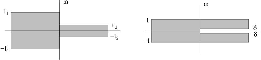
Figure 1: Schematic band structure of the uncoupled composite systems. Left: Metal-Metal, Right: Metal-Insulator.

It is simple to set up the eigenvalue problem for the full systems, and some details are given in the Appendix. However, the matching conditions in the center are difficult to handle in general. Therefore we determine the single-particle eigenvalues $\omega_{q}$ and the corresponding (real) eigenfunctions $\Phi_{q}(n)$ numerically. The correlation matrix $C_{mn}=\langle c^{{\dagger}}_{m}c_{n}\rangle$ is then

$$C_{mn}=\sum_{q\in F}\Phi_{q}(m)\Phi_{q}(n)$$ (6)

where the sum extends over the states $q$ in the Fermi sea. Restricting $C_{mn}$ to the chosen subsystem (either the left or the right half-chain), its eigenvalues $\zeta_{k}$ give the single-particle eigenvalues $\varepsilon_{k}=\ln[({1-\zeta_{k}})/{\zeta_{k}}]$ of the free-fermion entanglement Hamiltonian $\mathcal{H}$ in

$$\rho=\frac{1}{Z}\exp(-\mathcal{H})$$ (7)

where $\rho$ is the reduced density matrix Peschel03 . From them, the entanglement entropy $S$ follows as

$$S=\sum_{k}\ln(1+\mathrm{e}^{-\varepsilon_{k}})+\sum_{k}\frac{\varepsilon_{k}}{\mathrm{e}^{\varepsilon_{k}}+1}$$ (8)

In addition to the eigenvalues $\zeta_{k}$ resp. $\varepsilon_{k}$, we also determine the corresponding eigenfunctions $\varphi_{k}$ and construct $\mathcal{H}$ in section 4.

III Metal-metal system

We first consider half-filled systems where the Fermi level is in the middle of the bands. The resulting entanglement entropies for $t_{0}=1$ and three values of the parameter $\Delta$ are shown in Fig. 2, both for even and for odd $L$. One sees that the typical increase with the size, known for the homogeneous case $\Delta=0$, persists in the composite systems. The plot against lnL shows that also the asymptotic law $1/6\ln L+k$ is unchanged. However, the value of $k$ becomes smaller and the finite-size effects, in particular the even-odd alternation, increase dramatically as $\Delta$ becomes larger. For $\Delta=3$ (not shown), the values of $S$ are initially close to zero and to $\ln 2$, respectively. In this case, the ratio of the bandwidths $t_{2}/t_{1}\simeq 1/400$ is already very small, the states localized on the left drop rapidly on the right, while the extended states have very small amplitudes on the left (see the Appendix). For even $L$, this leads to a small entanglement which only increases as more states come into play at larger $L$. The value $\ln 2$ for odd $L$ is a consequence of the particle-hole symmetry of the problem which, in this case, forces one of the $\varepsilon_{k}$ to vanish.

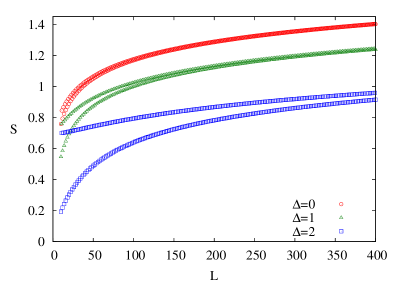
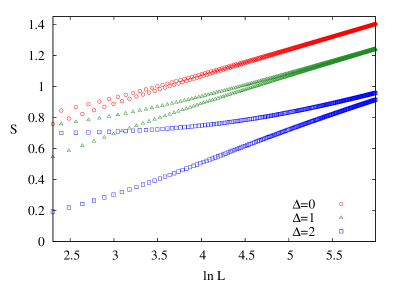
Figure 2: Entanglement entropy $S$ for $\Delta_{0}=0$ and three values of $\Delta$. Left: as function of $L$. Right: as function of $\ln L$. The upper (lower) curves correspond to odd (even) values of $L$.

The function $S(L,\Delta)$ has an intriguing universal behaviour. If one defines a length $L^{*}=L/\alpha$ and chooses the scale factor $\alpha$ properly, one can achieve $S(L^{*},\Delta)=S(L,0)$, i.e. all curves collapse on the one for the homogeneous system. Written differently, one has

$$S(L,\Delta)=S(\alpha L,0)$$ (9)

In the asymptotic region, where one has straight lines in a logarithmic plot, this feature is not surprising: A rescaling can always generate the necessary shift to make the curves coincide. However, the phenomenon is not restricted to this region. As shown in Fig. 3 on the left, it also holds for small sizes where there is still curvature in the graph. The variation of $\alpha$ with $\Delta$ is given on the right hand side of Fig. 3. One sees that the results determined from different (even) $L$ agree very well and that $\alpha$ becomes rapidly smaller as $\Delta$ increases. The curve can be described approximately by $1/\mathrm{ch}^{2}\,\Delta$. Note that the relation (9) can only be applied to values of $L$ such that $\alpha L$ is larger than 1.

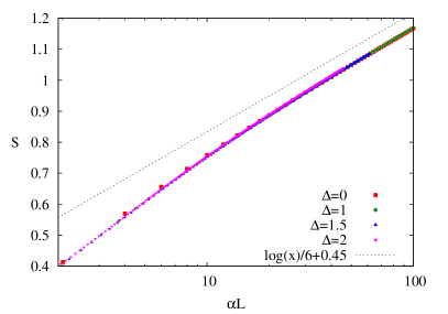
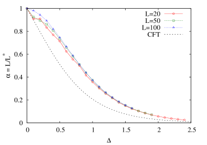
Figure 3: Scaling behaviour of the entanglement entropy. Left: $S$ as a function of the effective length $\alpha L$ for four values of $\Delta$ (logarithmic scale). Right: Variation of $L/L^{*}=\alpha$ with $\Delta$. The dotted line is the conformal factor in (10).

At this point, an observation from the appendix is helpful. Namely, near the Fermi level the wavefunctions in the right subsystem are the same as for a homogeneous system of total length $L(1+r)$. Thus, ignoring the states outside the narrow band, the correlation matrix on the right is the same as for an unsymmetrically divided homogenous chain and one can invoke the conformal result for the entropy CC04 extended in Fagotti/Calabrese11 to include $1/L$ corrections. This gives

$$S_{FC}=\frac{1}{6}\ln z-\frac{(-1)^{\ell}}{z}+\mathrm{const.},\quad\quad z=\frac{4}{\pi}L(1+r)\sin{\frac{\pi\ell}{L(1+r)}},$$ (10)

with $\ell=L$. The $r$-dependent factor in $z$ provides a similar rescaling of $L$ as $\alpha$, and a corresponding shift of the curves. It turns out, however, that this is not enough to make them coincide. Rather, one has a residual difference $S-S_{FC}=S_{I}(\Delta)$, which one can attribute to the interface, and which rises smoothly from $0$ to about $0.13$ as $\Delta$ increses from $0$ to $3$. It has its origin in the neglected exponentially decaying states below the narrow band.

This can be seen clearly, if one considers a partition of the system with $\ell<L$ sites on the right and calculates the entanglement between this subsystem and the remainder. As demonstrated in Fig. 4, the expression (10) then fits the data very well as soon as one moves away from the interface by a few lattice sites. One can also consider a division located in the left part of the system where the extended wave functions are the same as in a homogeneous system with total length $L(1+1/r)$, but in this case the conformal formula does not work well because the additional states are more important. These results also show that the symmetrical division is actually a somewhat special case.

\psfrag{l}[.9]{$\ell$}\includegraphics[scale={.8}]{figs2/ent_l_theta_thetanull0_L100_cft.eps}

Figure 4: Entanglement entropy between the outermost $\ell$ sites of the right subsystem and the remainder for $L=100$ and three values of $\Delta$. The inset shows the deviation from the formula (10).

We now turn to the effect of $t_{0}$. If one varies the central bond in a homogeneous chain ($\Delta=0$), the asymptotic behaviour of $S$ is

$$S=\frac{c_{\mathrm{eff}}}{6}\ln L+k$$ (11)

where $c_{\mathrm{eff}}$ depends on $t_{0}$ and is given by an explicit, though lengthy formula in which only the transmission coefficient at the Fermi energy $T\equiv s^{2}$ enters Eisler/Peschel10 . But the calculation in the Appendix shows that $T$ is independent of $\Delta$ and given by

$$T=\frac{1}{\mathrm{ch}^{2}\,\Delta_{0}}$$ (12)

Therefore one expects the result of the homogeneous problem also in the composite systems. This is, in fact, the case and demonstrated in Fig. 5 on the left, where results obtained by fitting the data between $L=100$ and $L=400$ to (11) plus a $1/L$ term are collected. For $\Delta=2$, the average between even and odd sizes was taken, while for $\Delta=1$ this was unnecessary. This verifies the Fermi-edge character of $c_{\mathrm{eff}}$ also in the present case.

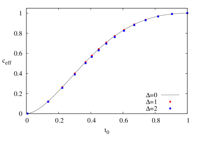
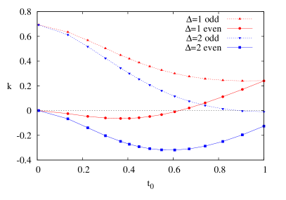
Figure 5: Effective central charge $c_{\mathrm{eff}}$ and constant $k$ in (11) as functions of $t_{0}$ for different values of $\Delta$. The line $\Delta=0$ in the left figure is the theoretical result, see Eisler/Peschel10 .

The constant $k$, on the other hand, depends on $\Delta$, as was found above already for the special case $t_{0}=1$. It is shown in Fig. 5 on the right. The values for odd $L$ are always larger than those for even $L$ with the maximal difference of $\ln 2$ appearing for $t_{0}\rightarrow 0$. This is connected with the half-integer particle number in each subsystem for odd $L$ which leads to a kind of singlet state even in the decoupling limit. The minimum in $k$ for even $L$ is also present for $\Delta=0$ and was also found for a segment in an infinite chain Peschel05 .

Finally, we consider the dependence of $S$ on the filling $\nu=N/2L$ of the system, where $N$ is the number of particles. It is shown in Fig. 6 for a fixed length $L=200$ and four values of $\Delta$. The smooth curve (red) is the result for the homogeneous system and given, up to the small even-odd oscillations Laflorencie/etal06 ; Affleck/Laflorencie/Sorensen09 ; Calabrese/Essler10 ; Fagotti/Calabrese11 and a constant, by $1/6\ln(\sin{q_{F}})$, where $q_{F}=\pi\nu$ Jin/Korepin04 . Turning on $\Delta$, regions of very small entanglement develop for small and large filling, where only states localized on the left are occupied or remain empty. At the same time, the oscillations of $S$ in the central region become slower and slower.

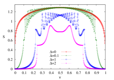
Figure 6: Entanglement entropy $S$ as a function of the filling $\nu=N/2L$ for $L=200$ and different $\Delta$.

The origin of these oscillations, at the level of the eigenvalues $\varepsilon_{k}$, can be seen in Fig. 7. There, the low-lying $\varepsilon_{k}$ are shown for all fillings between $0.2$ and $0.8$. For the case $\Delta=2$, shown on the right, the variation of the $\varepsilon_{k}$ with $\nu$ is rather slow and the curves cross zero only at two fillings. At these points, the crossing eigenvalue gives the maximal contribution to $S$, namely $\ln 2$, and they coincide with the locations of the maxima in Fig. 6. For $\Delta=1$, shown on the left, the variation is much faster and one has altogether 16 crossings. This is again the number of maxima of $S$ in the center of Fig. 6.

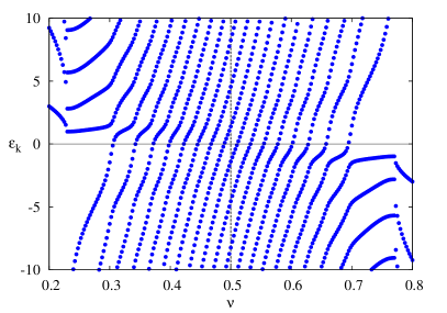
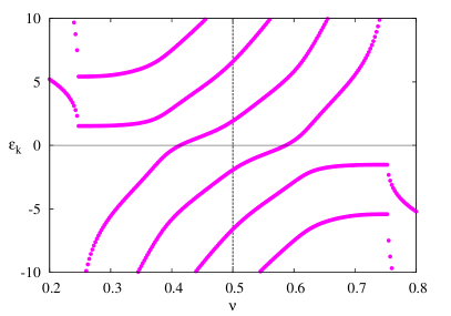
Figure 7: Variation of the low-lying single-particle eigenvalues $\varepsilon_{k}$ with the filling $\nu=N/2L$ for $L=200$. Left: $\Delta=1$. Right: $\Delta=2$. The colours are the same as in Fig. 6.

These structures can again be understood from the relation to a smaller, unsymmetrically divided homogeneous system. In such a case, if $L^{\prime}$ is the size of the smaller subsystem, one has $L^{\prime}$ crossings of the eigenvalues and the effect on $S$ is given by a factor $\sin{(q_{F}(2L^{\prime}+1))}/\sin{q_{F}}$ replacing the alternating sign of the $1/z$ term in (10). This leads to slow oscillations, although less pronounced than the observed ones. However, $L^{\prime}=rL$ gives $L^{\prime}=3.6$ for $\Delta=2$ and $L^{\prime}=27$ for $\Delta=1$ and thus not the correct numbers (2 and 16), even if one takes the nearest integer. But one can argue that the length $rL$ only refers to the states in the center of the band, while near the edges $\sin{k_{2}}$ appears in (26) which is smaller than $k_{2}$ by a factor of $2/\pi$. Working with $\tilde{L^{\prime}}=2rL/\pi$ gives values $2.3$ and $17.2$, respectively, which are quite close to the numerical findings. One also arrives at $\tilde{L^{\prime}}$ by counting the number of levels which the left subsystem contributes to the total number of band states. To accommodate them, one needs just this number of additional sites.

One should mention that one can see basically the same structures also in the energy $\omega$ as tiny deviations from the otherwise smooth level spacing of the extended states. In this case, the interpretation is that $\tilde{L^{\prime}}$ also gives the number of periods of the slowly varying tangent in (26) as $k_{2}$ sweeps through the band, and thus the number of possible peculiarities in the allowed momenta.

IV Metal-insulator system

In the following, we always consider half-filled systems. To avoid boundary states in the dimerized subsystem, we work with even $L$ and choose strong bonds $1+\delta$ at the borders. The entanglement entropies for two relatively small dimerizations and $t_{0}=1$ are shown in Fig. 8, together with those for the pure systems. One sees that the mixed system always has an intermediate entanglement, which is very plausible. Replacing one half of the metal by an insulator reduces the metallic result, while replacing one half of the insulator by a metal increases the insulator result.

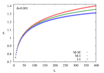
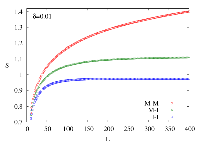
Figure 8: Entanglement entropies for metal-metal, metal-insulator and insulator-insulator systems as a function of $L$ for two values of the dimerization parameter $\delta$.

For $\delta=0.001$, shown on the left, all three curves look similar and there is no sign of a saturation, while for $\delta=0.01$ a saturation is clearly visible for the lower ones. This can be interpreted in terms of the correlation length $\xi=1/\delta$ in the insulator. It is $\xi=1000$ in the first case so that the non-criticality does not fully show up. In the second case, where $\xi=100$, it does and the crossover takes place roughly around this value.

In the region $L\ll\xi$, one can fit the curves for the composite system to a form $a\ln L+b$ and finds values of $a$ quite close to $1/6$. This can also be done for $t_{0}<1$ and gives curves for $c_{\mathrm{eff}}$ which lie somewhat below the metallic one shown in Fig. 5, but approach it as $\delta$ goes to zero. In the opposite limit, $L\gg\xi$, the entropy saturates and for $t_{0}=1$ one finds the asymptotic law $S\simeq 1/6\ln\xi+\mathrm{const.}$ as for the pure insulator but with a larger constant. To obtain the coefficient $1/6$ accurately from not too large $\xi$, one has to include subleading corrections of the form $(d\ln\xi+e)/\xi$ which one knows in the pure case from the connection to a transverse Ising chain sketched below. Again, the analysis can be extended to $t_{0}<1$, and in this case one finds $c_{\mathrm{eff}}$ to an accuracy of 3-4 digits.

On the level of the wavefunctions entering the correlation matrix, the (pseudo-) critical behaviour can be understood in the following way. For $L<\xi$ one has $|\omega|\sim 1/L>\delta$ and there are no states in the metal with energy in the band gap of the insulator and none in the insulator too close to the band edge. Thus one only has extended wavefunctions which are similar to those in the pure metal. This can be seen analytically or from the numerics.

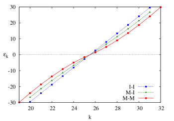
Figure 9: Eigenvalues $\varepsilon_{k}$ for metal-metal, metal-insulator and insulator-insulator systems with $L=50$ and $\delta=0.1$ for the insulator.

It is also instructive to look at the $\varepsilon_{k}$ spectra. In Fig. 9 an example is shown for the case $\delta=0.1$ and $L=50$. The lowest curve with the slight bend is the well- known result for the metal, while the highest one is for the insulator and strictly linear as for the transverse Ising chain or the XY model review09 . In fact, one can find a relation between the $\varepsilon_{k}$ for the dimerized hopping model and the transverse Ising chain using the method in Igloi/Juhasz08 . The latter model then has field $h=1$ and coupling $\lambda=(1-\delta)/(1+\delta)$ and the $\varepsilon_{k}$ are

$$\varepsilon_{k}=(2k+1)\,\varepsilon,\quad\quad k=0,\pm 1,\pm 2,...,\quad\quad\varepsilon=\pi\,I(\lambda^{\prime})/I(\lambda)$$ (13)

where $I(\lambda)$ denotes the complete elliptic integral of the first kind and $\lambda^{\prime}=\sqrt{1-\lambda^{2}}$, see also Sirker14 . The MI result lies in between, with a small break after the first eigenvalue, which becomes more apparent for larger values of $\delta$, when the curve becomes steeper and more linear.

For the spectrum, it does not matter in which of the two subsystems one considers the correlation matrix. Formally, this follows from the property $C^{2}=C$ for the full system Turner/Zhang/Vishwanath09 . However, the eigenvectors of the two reduced matrices, and therefore the corresponding entanglement Hamiltonians $\mathcal{H}$, are quite different. This is illustrated in Fig. 10 for the lowest $|\varepsilon_{k}|$ and $\delta=0.1$. We have plotted $\varphi_{k}(n)$ for $+\varepsilon_{k}$ on the left and for $-\varepsilon_{k}$ on the right, since these two are directly related. Namely, if one partitions $C$ into four blocks according to the location of the sites and $\varphi^{1}$ is an eigenvector of $C^{11}$ for part 1 with eigenvalue $\zeta$, then

$$\varphi^{2}=C^{21}\varphi^{1}$$ (14)

is an eigenvector of $C^{22}$ for part 2 with eigenvalue $1-\zeta$.

One sees the typical features of the pure systems on the two sides, namely a slow power-law decay in the metal (left) and a fast one within a distance $\xi=10$ in the insulator (right). The pure cases are shown for comparison, and one notes that the differences in the composite system are relatively small, lying more in the amplitudes than in the general behaviour.

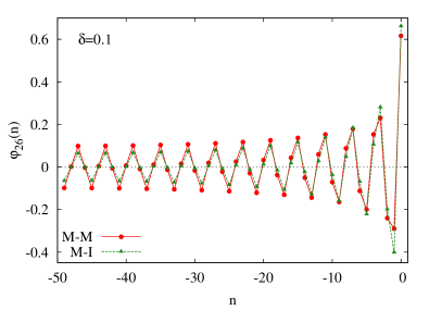
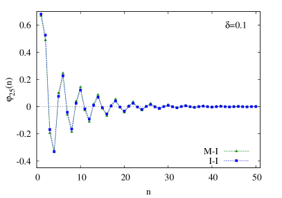
Figure 10: Eigenvectors of the MI correlation matrix for the smallest $|\varepsilon_{k}|$ in the metallic (left) and the insulating (right) subsystem for $L=50$ together with the results for the homogeneous cases (MM and II).

With the eigenvectors, one can explicitly determine the entanglement Hamiltonians $\mathcal{H}$. They have again the form of hopping models with basically only nearest-neighbour hopping as in $H$, but the amplitudes $\tilde{t}_{n}$ increase from the center towards the boundaries.

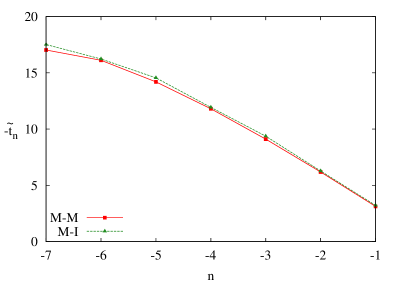
Figure 11: Nearest-neighbour hopping in the entanglement Hamiltonians for the left and right subsystem as a function of the position together with the results for the pure systems for $L=8$ and $\delta=0.1$.

In the pure metal, this increase is monotonous and the $\tilde{t}_{n}$ vary as $n(2L-n)$ review09 , while in the insulator one has an additional alternation which is coupled to the bond alternation in $H$. Due to the form of the eigenvectors, the result in the composite system is again close to that of the pure system on the corresponding side. This is shown in Fig. 11 for a system with a total of $2L=16$ sites, which is the largest size attainable before numerical errors in the large $\varepsilon_{k}$ set in.

V Evolution after a quench

In this section, we return to the metal-metal systems and study how the entanglement evolves after one joins the two initially disconnected parts. This type of local quench has been considered repeatedly in the past Eisler/Peschel07 ; CC07 ; EKPP07 ; Schoenhammer07 ; Klich/Levitov09 ; Stephan/Dubail11 ; Igloi/Szatmari/Lin12 ; Eisler/Peschel12 ; Collura/Calabrese13 ; Alba/HDM14 ; Kennes/Meden/Saleur14 ; Asplund/Bernamonti14 ; Chen/Vidal14 ; Thomas/Flindt15 . For the homogeneous case, one finds oscillations of $S(t)$ which one could call “entanglement bursts”, see e.g. Stephan/Dubail11 . In our case, the situation is more complex, because of the interface and the two Fermi velocities.

The two pieces are coupled at time $t=0$ by switching on $t_{0}$ and the evolution of $C(t)$ is calculated via the Heisenberg operators $c_{n}(t),c^{{\dagger}}_{n}(t)$. The resulting $S(t)$ is shown in Fig. 12 for two different values of $\Delta$ and of $t_{0}$. The system on the left with $\Delta=0.5$ has roughly the band widths of Fig. 1, while on the right the asymmetry is larger.

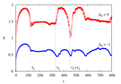
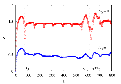
Figure 12: Evolution of the entanglement entropy $S$ after connecting two metallic systems with $L=100$. Left: $\Delta=0.5$. Right: $\Delta=1$. The times indicated are the theoretical values, see the text.

For $\Delta_{0}=0$ (upper curves) one has the following general features: An initial burst ending with a decrease at a time $\tau_{1}$ followed by a plateau, another burst at time $\tau_{2}$ which is a kind of mirror image of the first ending at time $\tau_{1}+\tau_{2}$ and then a rough repetition. For $\Delta=1$, the plateau is longer and shows six additional structures, whereas for $\Delta=0.5$ only a single one is visible. The lower curves have roughly the same pattern, but apart from the first maximum the structures are more washed out.

These features can be interpreted in the well-known picture due to Calabrese and Cardy CC05 , in which a pair of particles is emitted from the junction at time $t=0$, travelling in opposite directions and spreading the entanglement. In the present case, they have the velocities $v_{1}=t_{1}$ and $v_{2}=t_{2}$ and the corresponding space-time diagram is given in Fig. 13.

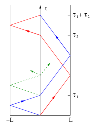
Figure 13: Trajectories of the particles in the Calabrese-Cardy picture.

After time $\tau_{1}=2L/v_{1}$, the left particle returns to the center, and if it simply moved into the right subsystem, the entanglement would continue to drop. This happens in a somewhat related situation where the velocities are the same, but the size of the right subsystem is larger Stephan/Dubail11 . Here, however, there is a probability for reflection at the interface, such that the entanglement rises again and another small “burst” follows. For $\Delta=1$, where $v_{1}=7.4\,v_{2}$, the left particle can make seven round trips before the right particle retuns to the center at time $\tau_{2}=2L/v_{2}=\tau_{1}/r$. These are very clearly visible in the Figure. There are, however, some remarks to make. According to (12) there is no reflection right at the Fermi level for $\Delta_{0}=0$. The effect can therefore only come from somewhat slower particles away from it. In fact, the numerical values for $\tau_{1}$ and $\tau_{2}$ are somewhat larger than the theoretical ones, which supports this argument. Also, one would expect the reflection effect to become weaker with each cycle, which is only barely the case. On the other hand, for $\Delta_{0}=-1$ one has $R=0.58$ at the Fermi level and the effect should be stronger, which is also not the case. Nevertheless, the picture gives a good overall description.

One could presume that at least the first burst can be described by the conformal result Stephan/Dubail11

$$S_{h}(vt)=\frac{c}{3}\ln{\left|\frac{2L}{\pi}\sin{\frac{\pi vt}{2L}}\right|}+\mathrm{const.}$$ (15)

valid for a homogeneous system with particle velocity $v$. Thus we tried the Ansatz

$$S(t)=[S_{h}(v_{1}t)+S_{h}(v_{2}t)]/2+\mathrm{const.}$$ (16)

which, on the scale of Fig. 12, fits the data for $\Delta_{0}=0$ very well. However, a closer look at the final decrease shows that it comes too early since, as mentioned, the value of $\tau_{1}$ is too small. Finally, we note that the first-burst results for a homogeneous but unequally divided system with the same round-trip times $\tau_{1}=2L_{1}$ and $\tau_{2}=2L_{2}$ lie above ours, and the difference increases with $\Delta$. Thus the two problems are not trivially connected.

VI Summary

We have considered the entanglement in fermionic chains composed of two different halves. In solid-state terminology, they were metals and insulators, while in statistical-physics terms they corresponded to critical and non-critical systems. The metal-metal system at half filling showed the same logarithmic behaviour of $S$ as a homogeneous chain with a defect. In the subleading terms, the asymmetry showed up, but the entropy had a remarkable scaling property. Its filling dependence, finally, showed oscillatory behaviour again linked to the asymmetry. Both features could be understood from the nature of the extended eigenfunctions which are the same as in homogeneous systems with different lengths.

The difference in the Fermi velocities showed up directly in the quench experiment where two half-filled metals were joined and the entanglement was monitored. In that case, the value of $r$ determined, how many cycles one sees in $S(t)$, before a certain return to the initial situation takes place. This pattern would occur in unsymmetrically divided homogeneous systems only with additional defects.

The metal-insulator system was somewhat simpler. Its entanglement properties were seen to lie always between the two pure systems and as a function of the size, one has a crossover from an initial critical behaviour with a logarithmic increase of the entanglement to a saturation typical for a non-critical system with finite correlation length. It also provided an instructive example for entanglement Hamiltonians which are quite different for the two subsystems although they have the same spectra, as they must. One should note that the dimerized hopping model used for the insulator, and investigated already in Sirker14 , plays a central role in the theory of polyacetylene Su/Schrieffer/Heeger79 ; Su/Schrieffer/Heeger80 . In that sense, we studied a particular polymer system.

We considered the geometry with open ends, because then one has only a single interface. However, one could equally well look at rings. For composite transverse Ising models this was done first in Hinrichsen90 ; Berche/Turban90 but without particular interface bonds and with a view on the spectra. Obtaining the entanglement entropy is more complicated, and we could only give an analytical result for the asymptotic behaviour of the metal-metal system.

While we focussed on the entanglement entropy, it is known that the particle-number fluctuations in the subsystems behave similarly Song12 . Thus, in a homogeneous metal, the prefactor of the $\ln L$ term in the fluctuations is given by $T/2\pi^{2}$ with the transmission coefficient $T$ CMV12a and varies qualitatively like $c_{\mathrm{eff}}$. The same result is found in the composite systems, and this could offer a way to access the entanglement experimentally.

Appendix: Some formulae for the metal-metal system

Let $\bar{\phi}(n)$ and $\phi(n)$ denote the wave function at site $n$ on the left and right, respectively. The bulk solutions on the two sides are waves with momenta $q_{1}$ and $q_{2}$ and energy $\omega=-t_{1}\cos{q_{1}}=-t_{2}\cos{q_{2}}$. At the interface, the equations are

$$t_{0}\,\bar{\phi}(0)=t_{2}\,\phi(0)\quad,\quad t_{1}\,\bar{\phi}(1)=t_{0}\,\phi(1)$$ (17)

For a wave coming in from the left and being partially reflected and transmitted, the amplitudes are

$$\begin{split}\bar{\phi}(n)&=A_{1}\exp{(iq_{1}n)}+B_{1}\exp{(-iq_{1}n)}\\ \phi(n)&=A_{2}\exp{(iq_{2}n)}\end{split}$$ (18)

Inserting this into the relations (17), one finds for the reflection coefficient

$$R=\left|\frac{B_{1}}{A_{1}}\right|^{2}=\frac{\mathrm{ch}\,2\nu-\cos{(q_{1}-q_{2})}}{\mathrm{ch}\,2\nu-\cos{(q_{1}+q_{2})}}$$ (19)

where the quantity $\nu$ is defined as $\exp{(2\nu)}=t_{0}^{2}/t_{1}t_{2}$. In our parametrization, where $t_{1}t_{2}=1$, one has $\nu=\Delta_{0}$. The transmission coefficient follows from $T=1-R$ and can be written

$$T=\frac{\sin{q_{1}}\sin{q_{2}}}{\mathrm{sh}^{2}\,\nu+\sin^{2}{((q_{1}+q_{2})/2)}}$$ (20)

If the left and right subsystems are identical, $q_{1}=q_{2}=q$, and one finds the result for a bond defect in an otherwise homogeneous chain. The same holds in a general system if one is in the middle of the bands. Then $\omega=0,q_{1}=q_{2}=\pi/2$ and one has the result

$$T=\frac{1}{\mathrm{ch}^{2}\,\nu}$$ (21)

Due to the factor $\sin{q_{2}}$ in (20), the transmission vanishes at the edges of the narrow band.

The extended eigenfunctions of $H$ have the form

$$\bar{\phi}(n) = A_{1}\sin{q_{1}(n+L)}$$

$$\phi(n) = A_{2}\sin{q_{2}(n-L-1)}$$ (22)

and the conditions (17) lead to

$$\frac{\sin{q_{1}(L+1)}\;\sin{q_{2}(L+1)}}{\sin{q_{1}L}\;\sin{q_{2}L}}=\frac{t_{0}^{2}}{t_{1}t_{2}}$$ (23)

which, together with $t_{1}\cos{q_{1}}=t_{2}\cos{q_{2}}$, determines the allowed momenta. Setting $q_{\alpha}=\pi/2+k_{\alpha}$ and assuming $L$ even, it takes the form

$$\frac{\cos{k_{1}(L+1)}\;\cos{k_{2}(L+1)}}{\sin{k_{1}L}\;\sin{k_{2}L}}=\frac{t_{0}^{2}}{t_{1}t_{2}}$$ (24)

The relation between the $k_{\alpha}$ reads

$$\sin{k_{1}}=r\sin{k_{2}},\quad\quad r=t_{2}/t_{1}$$ (25)

and for small $r$ simplifies to $k_{1}=r\sin{k_{2}}$. Inserting this into (24) and setting $L+1\simeq L$ in the numerator then gives

$$\cot{(k_{2}L)}=\frac{t_{0}^{2}}{t_{1}t_{2}}\tan{(rL\sin{k_{2}})}$$ (26)

which contains only the momentum $k_{2}$. The solutions can be discussed graphically, but one sees directly that besides $L$ a second length $L^{\prime}=rL$ appears. If it is large enough, the tangent completes several cycles as $k_{2}$ varies, and this can lead to additional features in the momenta or in the amplitude ratio which is, again with $L+1\simeq L$,

$$\frac{A_{2}}{A_{1}}=-\frac{t_{1}}{t_{0}}\;\frac{\cos(rL\sin{k_{2}})}{\sin{k_{2}L}}$$ (27)

If $k_{2}$ is small, $k_{1}=rk_{2}$ for all $r<1$ and (26) for $t_{0}^{2}/t_{1}t_{2}=1$ can be written in the two forms

$$\tan{(k_{2}rL)}\tan{(k_{2}L)}=1,\quad\quad\tan{(k_{1}L)}\tan{(k_{1}L/r)}=1$$ (28)

Both equations are the same as for a homogeneous chain built up from two pieces with different lengths and can therefore be solved explicitly. For $k_{2}$, the homogeneous system has length $L+L^{\prime}$, while for $k_{1}$ it has length $L+L^{\prime\prime}$, where $L^{\prime\prime}=L/r$. Thus the small momenta are equidistant, i.e.

$$k_{2}=\frac{\pi}{2(L+L^{\prime})}\,(2n+1),\quad\quad n=0,\pm 1,\pm 2,...$$ (29)

Using (28) in (27), one finds $(A_{2}/A_{1})^{2}=t_{1}^{2}=1/r$, i.e. the amplitudes are larger on the right than on the left. Including normalization to leading order, this gives prefactors $A_{1}^{2}=2/(L+L^{\prime\prime})$ and $A_{2}^{2}=2/(L+L^{\prime})$ which correspond exactly to these chain lengths.

References

References

- (1) Peschel I and Eisler V 2009 J. Phys. A: Math. Theor. 42 504003
- (2) Peschel I 2005 J. Phys. A: Math. Gen. 38 4327
- (3) Iglói F, Szatmári Z and Lin Y-C 2009 Phys. Rev. B 80 024405
- (4) Eisler V and Peschel I 2010 Ann. Phys. (Berlin) 522 679
- (5) Eisler V and Garmon S S 2010 Phys. Rev. B 82, 174202
- (6) Peschel I and Eisler V 2012 J. Phys. A: Math. Theor. 45 155301
- (7) Calabrese P, Mintchev M and Vicari E 2011 Phys. Rev. Lett. 107 020601
- (8) Calabrese P, Mintchev M and Vicari E 2012 J. Phys. A: Math. Theor. 45 105206
- (9) Calabrese P, Mintchev M and Vicari E 2012 Europhys. Lett. 98 20003
- (10) Vasseur R, Jacobsen J L and Saleur H 2014 Phys. Rev. Lett. 112 106601
- (11) Eisler V and Peschel I 2007 J. Stat. Mech. P06005
- (12) Ossipov A 2014 Phys. Rev. Lett. 113 130402
- (13) Pouranvari M, Yang K and Seidel A 2015 Phys. Rev. B 91, 075115
- (14) Laflorencie N 2005 Phys. Rev. B 72 140408
- (15) Iglói F, Lin Y-C, Rieger H and Monthus C 2007 Phys. Rev. B 76 064421
- (16) Iglói F and Lin Y-C 2008 J. Stat. Mech. P06004
- (17) Hoyos J A, Laflorencie N, Viera A P and Vojta T 2011 Europhys. Lett. 93 30004
- (18) Iglói F, Juhász R and Zimborás Z 2007 Europhys. Lett. 79 37001
- (19) Vitagliano G, Riera A and Latorre J I 2010 New J. Phys. 12 113049
- (20) Ramirez G, Rodríguez-Laguna J and Sierra G 2014 J. Stat. Mech. P10004
- (21) Berkovits R 2012 Phys. Rev. Lett. 108 176803
- (22) Pastur L and Slavin V 2014 Phys. Rev. Lett. 113 150404
- (23) Pouranvari M, Zhang Y and Yang K 2015 Adv. Cond. Matter Phys. 397630
- (24) Eisler V, Iglói F and Peschel I 2009 J. Stat. Mech. P02011
- (25) Campostrini M and Vicari E 2010 Phys. Rev. A 81 023606
- (26) Campostrini M and Vicari E 2010 Phys. Rev. A 81 063614
- (27) Campostrini M and Vicari E 2010 J. Stat. Mech. P08020
- (28) Vicari E 2012 Phys. Rev. A 85 062104
- (29) Eisler V 2013 Phys. Rev. Lett. 111 080402
- (30) Eisler V and Peschel I 2014 J. Stat. Mech. P04005
- (31) Hinrichsen H 1990 Nucl. Phys. B 336 377
- (32) Berche B and Turban L 1990 J. Phys. A: Math. Gen. 24 245
- (33) Zhang D, Li B and Zhao M 1996 Phys. Rev. B 53 8161
- (34) Zhang D, Chen Z and Li B 1999 Chin. Phys. Lett. 16 44
- (35) Eisler V and Peschel I 2013 J. Stat. Mech. P04028
- (36) Calabrese P and Cardy J L 2005 J. Stat. Mech. P04010
- (37) Peschel I 2003 J. Phys. A: Math. Gen. 36 L205
- (38) Calabrese P and Cardy J L 2004 J. Stat. Mech. P06002
- (39) Fagotti M and Calabrese P 2011 J. Stat. Mech. P01017
- (40) Laflorencie N, Sørensen E S, Chang M-S and Affleck I 2006 Phys. Rev. Lett. 96 100603
- (41) Affleck I, Laflorencie N and Sørensen E S 2009 J. Phys. A: Math. Theor. 42 504009
- (42) Calabrese P and Essler F H L 2010 J. Stat. Mech. P08029
- (43) Jin B Q and Korepin V E 2004 J. Stat. Phys. 116 79
- (44) Iglói F and Juhász R 2008 Europhys. Lett. 81 57003
- (45) Sirker J, Maiti M, Konstantinidis N P and Sedlmayr N 2014 J. Stat. Mech. P10032
- (46) Turner A M, Zhang Y and Vishwanath A 2009 eprint arXiv:0909.3119
- (47) Calabrese P and Cardy J 2007 J. Stat. Mech. P10004
- (48) Eisler V, Karevski D, Platini T and Peschel I 2007 J. Stat. Mech. P01023
- (49) Schönhammer K 2007 Phys. Rev. B 76 205329
- (50) Klich I and Levitov L 2009 Phys. Rev. Lett. 102 100502
- (51) Stéphan J-M and Dubail J 2011 J. Stat. Mech. P08019
- (52) Iglói F, Szatmári Z and Lin Y-C 2012 Phys. Rev. B 85 094417
- (53) Eisler V and Peschel I 2012 Europhys. Lett. 99 20001
- (54) Collura M and Calabrese P 2013 J. Phys. A: Math. Theor. 46 175001
- (55) Alba V and Heidrich-Meisner F 2014 Phys. Rev. B 90 075144
- (56) Kennes D M, Meden V, Vasseur R 2014 Phys. Rev. B 90 115101
- (57) Asplund C T and Bernamonti A 2014 Phys. Rev. D 89 066015
- (58) Chen Y and Vidal G 2014 J. Stat. Mech. P10011
- (59) Thomas K H and Flindt C 2015 Phys. Rev. B 91 125406
- (60) Su W P, Schrieffer J R and Heeger A J 1979 Phys. Rev. Lett. 42 1698
- (61) Su W P, Schrieffer J R and Heeger A J 1980 Phys. Rev. B 22 2099
- (62) Song H F, Rachel S, Flindt C, Klich I, Laflorencie N and Le Hur K 2012 Phys. Rev. B 85 035409