thanks: corresponding author

Control of Multilayer Networks

Giulia Menichetti Department of Physics and Astronomy and INFN Sez. Bologna, Bologna University, Viale B. Pichat 6/2 40127 Bologna, Italy giulia.menichetti2@unibo.it    Luca Dall’Asta Department of Applied Science and Technology, DISAT, Politecnico di Torino, Corso Duca degli Abruzzi 24, 10129 Torino, Italy Collegio Carlo Alberto, Via Real Collegio 30, 10024 Moncalieri, Italy luca.dallasta@polito.it    Ginestra Bianconi School of Mathematical Sciences, Queen Mary University of London, London E1 4NS, United Kingdom ginestra.bianconi@gmail.com
Abstract

The controllability of a network is a theoretical problem of relevance in a variety of contexts ranging from financial markets to the brain. Until now, network controllability has been characterized only on isolated networks, while the vast majority of complex systems are formed by multilayer networks. Here we build a theoretical framework for the linear controllability of multilayer networks by mapping the problem into a combinatorial matching problem. We found that correlating the external signals in the different layers can significantly reduce the multiplex network robustness to node removal, as it can be seen in conjunction with a hybrid phase transition occurring in interacting Poisson networks. Moreover we observe that multilayer networks can stabilize the fully controllable multiplex network configuration that can be stable also when the full controllability of the single network is not stable.

Most of the real networks are not isolated but interact with each other forming multilayer structures PhysReports ; review2 . For example, banks are linked to each other by different types of contracts and relationships, gene regulation in the cell is mediated by the different types of interactions between different kinds of molecules, brain data are described by multilayer brain networks. Studying the controllability properties of these networks is important for assessing the risk of a financial crash Caldarelli ; Caldarelli2 , for drug discovery drug_discovery and for characterizing brain dynamics Bullmore ; Bonifazi ; brain ; Makse ; Remondini . Therefore the controllability of multilayer networks is a problem of fundamental importance for a large variety of applications.

Recently, linear Lin74 ; Liu ; correlations ; Ruths ; Reka ; PRL ; con_vicsek ; Spectrum ; Control_centrality and non-linear slotine ; con_pinning ; con_sorrentino ; con_boccaletti ; DiBernardo1 ; DiBernardo2 ; con_grebogi ; con_lai ; Motter ; Motter1 ; Lai2 approaches are providing new scenarios for the characterization of the controllability of single complex networks. In particular, in the seminal paper by Liu et al. Liu the structural controllability of complex networks has been addressed by mapping this problem into a Maximum Matching Problem that can be studied using statistical mechanics techniques Lenka ; Altarelli ; Cavity ; Zecchina ; Weigt ; Mezard . Other works approach the related problem of network observability observability , or target control target which focuses on controlling just a subset of the nodes. Despite the significant interest in network controllability, all linear and non-linear approaches for the controllability of networks are still restricted to single networks while it has been recently found that the multiplexity of networks can have profound effects on the dynamical processes taking place on them Havlin1 ; Havlin3 ; Doro1 ; BD ; Goh ; Diffusion . For example, percolation processes that usually present continuous phase transitions on single networks can become discontinuous on such structures Havlin1 ; Havlin3 ; Doro1 ; BD ; Goh and are characterized by large avalanches of disruption events.

Here, we consider the elegant framework of structural controllability Liu and investigate how the multilayer structure of networks can affect their controllability. We focus on multiplex networks, which are multilayer networks in which the same set of nodes are connected by different types of interactions. Multiplex network controllability is studied under the assumption that input nodes are the same in all network layers, thus mimicking the situation in which input nodes can send different signals in the different layers of the multiplex but the position of the external signals in the layers is correlated.

We show that controlling the dynamics of multiplex networks is more costly than controlling single layers taken in isolation. Moreover, the controllability of multiplex networks displays unexpected new phenomena. In fact these networks can become extremely sensible to damage in conjunction with a discontinuous phase transition characterized by a jump in the number of input points (driver nodes). A careful investigation of this phase transition reveals that this is a hybrid phase transition with a square root singularity, therefore in the same universality class of the emergence of the mutually connected component in multiplex networks Havlin1 ; Doro1 ; PhysReports . The number of driver nodes in the multiplex network is in general higher than the number of driver nodes in the single layers taken in isolation. Nevertheless the degree correlations between low-degree nodes in the different layers can affect the controllability of the multiplex network and modulate the number of its driver nodes. Moreover, a fully controllable configuration can be stable in a multilayer network even if it is not stable in the isolated networks that form the multilayer structure.
Refer to caption
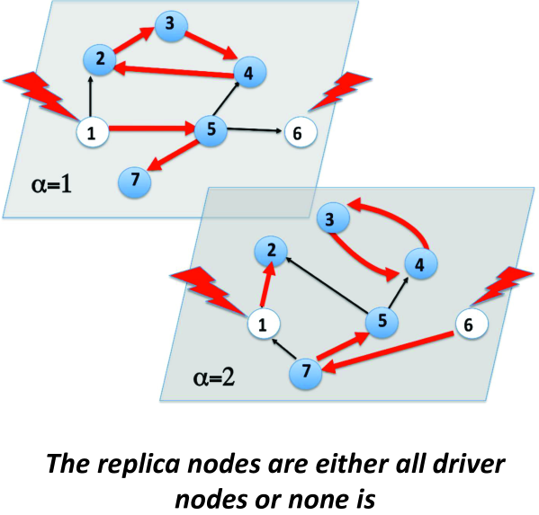
Figure 1: Control of a multiplex network. The controllability of a duplex network (multiplex with M=2𝑀2M=2 layers) can be mapped to a Maximum Matching Problem in which the unmatched nodes (indicated with a white circle) are the driver nodes of the duplex network. Here we have indicated with red thick links the matched links and by black thin links the unmatched links.

RESULTS

We consider multiplex networks PhysReports in which every node i=1,2,,N𝑖12𝑁i=1,2,\ldots,N has a replica node (i,α)𝑖𝛼(i,\alpha) in each layer α𝛼\alpha and every layer is formed by a directed network between the corresponding replica nodes. We assume that each replica node (i,α)𝑖𝛼(i,\alpha) is characterized by a different dynamical variable xiαRsuperscriptsubscript𝑥𝑖𝛼Rx_{i}^{\alpha}\in\mathrm{R} and that each layer is characterized by a possibly different dynamical process. We consider for simplicity a duplex, i.e a multiplex formed by two layers {A,B}𝐴𝐵\{A,B\} where each layer α{A,B}𝛼𝐴𝐵\alpha\in\{A,B\} is a directed network. The state of the network at time t𝑡t is governed by a linear dynamical system

d𝐗(t)dt=𝒢𝐗+𝒦𝐮,𝑑𝐗𝑡𝑑𝑡𝒢𝐗𝒦𝐮\displaystyle\frac{d{\bf X}(t)}{dt}={\cal G}{\bf X}+{\cal K}{\bf u}, (1)

in which the 2N2𝑁2N-dimensional vector 𝐗(t)𝐗𝑡{\bf X}(t) describes the dynamical state of each replica node, i.e. Xi=xiAsubscript𝑋𝑖superscriptsubscript𝑥𝑖𝐴X_{i}=x_{i}^{A} and XN+i=xiBsubscript𝑋𝑁𝑖superscriptsubscript𝑥𝑖𝐵X_{N+i}=x_{i}^{B} for i=1,2,,N𝑖12𝑁i=1,2,\ldots,N. The matrix 𝒢𝒢{\cal G} is a 2N×2N2𝑁2𝑁2N\times 2N (asymmetric) matrix and 𝒦𝒦{\cal K} is a 2N×P2𝑁𝑃2N\times P matrix. They have the following block structure

𝒢=(gA00gB),𝒦=(KA00KB),formulae-sequence𝒢superscript𝑔𝐴0missing-subexpressionmissing-subexpression0superscript𝑔𝐵missing-subexpressionmissing-subexpression𝒦superscript𝐾𝐴00superscript𝐾𝐵\displaystyle{\cal G}=\left(\begin{array}[]{cccc}g^{A}&0\\ 0&g^{B}\end{array}\right),\ \ \ {\cal K}=\left(\begin{array}[]{cc}K^{A}&0\\ 0&K^{B}\end{array}\right), (6)

in which gαsuperscript𝑔𝛼g^{\alpha} are the N×N𝑁𝑁N\times N matrices describing the directed weighted interactions within the layers and Kαsuperscript𝐾𝛼{K}^{\alpha} are the N×Pα𝑁superscript𝑃𝛼N\times P^{\alpha} matrices describing the coupling between the nodes of each layer α𝛼\alpha and PαNsuperscript𝑃𝛼𝑁P^{\alpha}\leq N external signals. The latter are represented by a vector 𝐮(t)𝐮𝑡{\bf u}(t) of elements uγsubscript𝑢𝛾u_{\gamma} and γ=1,2P=PA+PBformulae-sequence𝛾12𝑃superscript𝑃𝐴superscript𝑃𝐵\gamma=1,2\ldots P=P^{A}+P^{B}. Here we consider the concept of structural controllability Lin74 ; Liu that guarantees the controllability of a networks for any choice of the non-zeros entries of 𝒢𝒢{\cal G} and 𝒦𝒦{\cal K}, except for a variety of zero Lebesgue measure in the parameter space. Therefore each layer of the duplex networks can be structurally controlled by identifying a minimum number of driver nodes, that are controlled nodes which do not share input vertices. If different replicas of the same node can be independently controlled, then the controllability properties of the multiplex network factorize and each layer can be studied as if was taken in isolation slotine ; Lin74 ; Liu ; PRL . Liu et al. Liu showed that in a single layer the minimum set of driver nodes can be found by mapping the problem into a matching problem. In real multiplex networks however nodes are usually univocally defined and share common properties across different layers, therefore we make the assumption that each node of the duplex network is either a driver node in each layer or it is not a driver node in any layer. The problem of finding the driver nodes of the duplex network can be thus mapped into a maximum matching problem in which every node has at most one matched incoming link and at most one matched outgoing link, with the constraint that two replica nodes either have no matched incoming links on each layer or have one matched incoming link in each layer (see Figure 1). This problem can be studied, using statistical mechanics techniques, such as the cavity method and the Belief Propagation (BP) algorithm. Following Liu ; PRL , we consider the variables sijα=1,0superscriptsubscript𝑠𝑖𝑗𝛼10s_{ij}^{\alpha}=1,0 indicating respectively if the directed link from node (i,α)𝑖𝛼(i,\alpha) to node (j,α)𝑗𝛼(j,\alpha) in layer α=A,B𝛼𝐴𝐵\alpha=A,B is matched or not. In order to have a matching in each layer of the duplex the following constraints have always to be satisfied

j+αisijα1,iαjsijα1.formulae-sequencesubscript𝑗superscriptsubscript𝛼𝑖superscriptsubscript𝑠𝑖𝑗𝛼1subscript𝑖superscriptsubscript𝛼𝑗superscriptsubscript𝑠𝑖𝑗𝛼1\displaystyle\sum_{j\in\partial_{+}^{\alpha}i}s_{ij}^{\alpha}\leq 1,\ \ \ \sum_{i\in\partial_{-}^{\alpha}j}s_{ij}^{\alpha}\leq 1. (7)

where +αisuperscriptsubscript𝛼𝑖\partial_{+}^{\alpha}i is the set of replica nodes (j,α)𝑗𝛼(j,\alpha) in layer α𝛼\alpha that are reached by directed links from (i,α)𝑖𝛼(i,\alpha) and αjsuperscriptsubscript𝛼𝑗\partial_{-}^{\alpha}j is the set of replica nodes (i,α)𝑖𝛼(i,\alpha) in layer α𝛼\alpha that point to (j,α)𝑗𝛼(j,\alpha). In addition, we impose that the driver nodes in the two layers (the unmatched nodes) are replica nodes, i.e.

iAjsijA=iBjsijB.subscript𝑖superscriptsubscript𝐴𝑗superscriptsubscript𝑠𝑖𝑗𝐴subscript𝑖superscriptsubscript𝐵𝑗superscriptsubscript𝑠𝑖𝑗𝐵\displaystyle\sum_{i\in\partial_{-}^{A}j}s_{ij}^{A}=\sum_{i\in\partial_{-}^{B}j}s_{ij}^{B}. (8)

In this formalism, computing the maximum matching corresponds to minimize an energy function E=ND=NnD𝐸subscript𝑁𝐷𝑁subscript𝑛𝐷E=N_{D}=Nn_{D} where NDsubscript𝑁𝐷N_{D} is the number of unmatched replica nodes associated to each matching. The energy E𝐸E for a given matching, can be expressed in terms of the variables sijsubscript𝑠𝑖𝑗s_{ij} as

E𝐸\displaystyle E =\displaystyle= αj(1iαjsijα).subscript𝛼subscript𝑗1subscript𝑖superscriptsubscript𝛼𝑗superscriptsubscript𝑠𝑖𝑗𝛼\displaystyle\sum_{\alpha}\sum_{j}\left(1-\sum_{i\in\partial_{-}^{\alpha}j}s_{ij}^{\alpha}\right). (9)

In order to study this novel statistical mechanics problem, we derived the BP equations Mezard ; Cavity ; Weigt (see Methods and Supplementary Material) valid in the locally tree-like approximation, as described for the case of a single network problem in Lenka ; Altarelli ; Zecchina ; Liu ; PRL .
Refer to caption
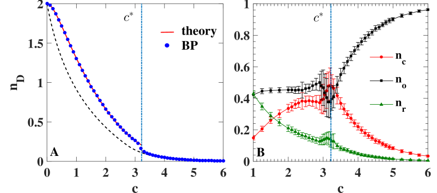
Figure 2: Controllability of Poisson duplex networks with average degrees kA,in=kA,out=kB,in=kB,out=cdelimited-⟨⟩superscript𝑘𝐴𝑖𝑛delimited-⟨⟩superscript𝑘𝐴𝑜𝑢𝑡delimited-⟨⟩superscript𝑘𝐵𝑖𝑛delimited-⟨⟩superscript𝑘𝐵𝑜𝑢𝑡𝑐\left\langle{k^{A,in}}\right\rangle=\left\langle{k^{A,out}}\right\rangle=\left\langle{k^{B,in}}\right\rangle=\left\langle{k^{B,out}}\right\rangle=c. In panel A the fraction nDsubscript𝑛𝐷n_{D} of driver nodes in a Poisson duplex network with kA,in=kA,out=kB,in=kB,out=cdelimited-⟨⟩superscript𝑘𝐴𝑖𝑛delimited-⟨⟩superscript𝑘𝐴𝑜𝑢𝑡delimited-⟨⟩superscript𝑘𝐵𝑖𝑛delimited-⟨⟩superscript𝑘𝐵𝑜𝑢𝑡𝑐\left\langle{k^{A,in}}\right\rangle=\left\langle{k^{A,out}}\right\rangle=\left\langle{k^{B,in}}\right\rangle=\left\langle{k^{B,out}}\right\rangle=c, plotted as a function of the average degree c𝑐c. The points indicate the average BP results obtained over 5 single realizations of the Poisson duplex networks with average degree c𝑐c and N=104𝑁superscript104N=10^{4}, the solid line is the theoretical expectation (the error bar, indicating the interval of one standard deviation from the mean, is always smaller or comparable to marker size). The dashed line represents twice the density of driver nodes for a single Poisson network with the same average degree.
In panel B the densities nc,nrsubscript𝑛𝑐subscript𝑛𝑟n_{c},n_{r} and nosubscript𝑛𝑜n_{o} respectively of critical redundant and ordinary nodes are shown as functions of c𝑐c for the same type of duplex networks with N=103𝑁superscript103N=10^{3}, where each point is the average over 100 different instances.
In both panels the dot-dashed vertical line indicates the phase transition average degree c=3.222326106superscript𝑐3.222326106c^{*}=3.222326106\ldots.
Refer to caption
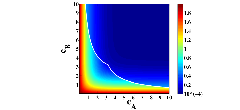
Figure 3: Phase diagram of the controllability for a Poisson duplex networks with average degrees kA,in=kA,out=cAdelimited-⟨⟩superscript𝑘𝐴𝑖𝑛delimited-⟨⟩superscript𝑘𝐴𝑜𝑢𝑡subscript𝑐𝐴\left\langle{k^{A,in}}\right\rangle=\left\langle{k^{A,out}}\right\rangle=c_{A} and kB,in=kB,out=cBdelimited-⟨⟩superscript𝑘𝐵𝑖𝑛delimited-⟨⟩superscript𝑘𝐵𝑜𝑢𝑡subscript𝑐𝐵\left\langle{k^{B,in}}\right\rangle=\left\langle{k^{B,out}}\right\rangle=c_{B}. The color code indicates the density of driver nodes nD=E/Nsubscript𝑛𝐷𝐸𝑁n_{D}=E/N in the multiplex network.

DISCUSSION

The controllability of multiplex networks displays a rich phenomenology, coming from the interplay between the dynamical and the structural properties of multiplex networks. Here we characterize the controllability of multiplex networks with different degree distribution and with tunable level of structural correlations.

Phase transition in Poisson duplex networks–

We consider duplex networks in which the two layers are realizations of uncorrelated directed random graphs characterized by Poisson distributions for in-degree and out-degree with same average value c𝑐c, i.e. kinA=koutA=kinB=koutB=cdelimited-⟨⟩subscriptsuperscript𝑘𝐴𝑖𝑛delimited-⟨⟩subscriptsuperscript𝑘𝐴𝑜𝑢𝑡delimited-⟨⟩subscriptsuperscript𝑘𝐵𝑖𝑛delimited-⟨⟩subscriptsuperscript𝑘𝐵𝑜𝑢𝑡𝑐\langle{k^{A}_{in}}\rangle=\langle{k^{A}_{out}}\rangle=\langle{k^{B}_{in}}\rangle=\langle{k^{B}_{out}}\rangle=c. In Figure 2A we report the average rescaled number of driver nodes nDsubscript𝑛𝐷n_{D} as function of the average degree c𝑐c computed from the solutions of Eqs.(12) on single instances and from the graph ensemble analysis. A comparison with two independent layers with the same topological properties shows that the controllability of a duplex network is in general more demanding in terms of number of driver nodes than the controllability of independent single layers, in particular for low average degrees. In addition, a discontinuity in the number of driver nodes at c=c=3.2223𝑐superscript𝑐3.2223c=c^{\star}=3.2223\ldots marks a change in the controllability properties of duplex networks that is not observed in uncoupled networks. This is due to a structural change in the solution of the matching problem, in which a finite density of zero valued cavity fields emerges. A careful investigation (see Supplementary Material ) reveals that this is a hybrid phase transition with a square root singularity, therefore in the same universality class of the emergence of the mutually connected component in multiplex networks Havlin1 ; Doro1 ; PhysReports .

In correspondence to this phase transition the network responds non trivially to perturbations. This is observed by performing a numerical calculation of the robustness of the networks. Following Liu we classify the nodes into three categories: critical nodes, redundant nodes and ordinary nodes. When a critical node is removed from the (multiplex) network, controllability is sustained at the cost of increasing the number of driver nodes. If the number of driver nodes decreases or is unchanged, the removed nodes are classified as redundant and ordinary respectively. Figure 2B shows that the fraction of critical nodes reaches a maximum at the transition, revealing an increased fragility of the duplex network to random damage with respect to single layers. While an abrupt change in the number of driver nodes can result from a small change in the network topology, it is important to stress that the non-monotonic behavior of these quantities around the critical average degree value could be interpreted as a precursor of the discontinuity.

In a duplex network formed by directed Poisson random graphs with different average degree in the two layers (i.e. kinα=koutα=cαdelimited-⟨⟩subscriptsuperscript𝑘𝛼𝑖𝑛delimited-⟨⟩subscriptsuperscript𝑘𝛼𝑜𝑢𝑡subscript𝑐𝛼\langle{k^{\alpha}_{in}}\rangle=\langle{k^{\alpha}_{out}}\rangle=c_{\alpha}) a similar discontinuous phase transition is observed (see Figure 3). Nevertheless we checked that this discontinuous phase transition is not occurring for every multiplex network structure (see Supplementary Material).
Refer to caption
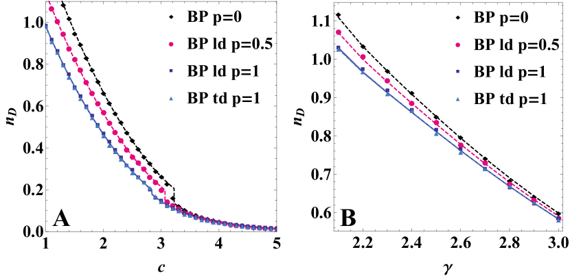
Figure 4: The effect of the degree correlation between replica nodes in different layers on the controllability of multiplex networks. Correlations between the low in-degrees (ld) and correlations between any in-degree node (td), parametrized by p𝑝p, affect the fraction of driver nodes in the network nDsubscript𝑛𝐷n_{D}, both in the case of Poisson networks with the same in and out average degree c𝑐c across the two layers (Panel A) and in the case of scale-free networks with the same in and out degree distribution across the layers, given by P(k)kγproportional-to𝑃𝑘superscript𝑘𝛾P(k)\propto k^{-\gamma} and minimum in/out degree 111 (Panel B). When p=0𝑝0p=0 there is no degree correlation between replica nodes in different layers. The BP data are shown for networks with N=104𝑁superscript104N=10^{4}, and are averaged 5 times for panel A and 20 times for panel B.
Refer to caption
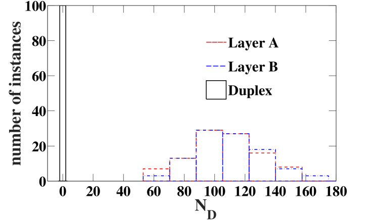
Figure 5: The fully controllable solution can be stable for the multiplex network also if it is not stable for the single layers taken in isolation. Histogram of the number of networks that out of 100 realizations have NDsubscript𝑁𝐷N_{D} driver nodes. The results obtained for the control of a duplex networks and its two layers are compared. The duplex networks are formed by two scale-free networks with N=104𝑁superscript104N=10^{4} and PA,in(k)=PB,inkγsuperscript𝑃𝐴𝑖𝑛𝑘superscript𝑃𝐵𝑖𝑛proportional-tosuperscript𝑘𝛾P^{A,in}(k)=P^{B,in}\propto k^{-\gamma} for k>2𝑘2k>2 and PA,out(k)=PB,out(k)kγsuperscript𝑃𝐴𝑜𝑢𝑡𝑘superscript𝑃𝐵𝑜𝑢𝑡𝑘proportional-tosuperscript𝑘𝛾P^{A,out}(k)=P^{B,out}(k)\propto k^{-\gamma} for k>2𝑘2k>2, with γ=2.3𝛾2.3\gamma=2.3, the networks have minimum in-degree equal to 2 and minimum out-degree equal to 3 and PA,in(2)=PB,in(2)=0.3superscript𝑃𝐴𝑖𝑛2superscript𝑃𝐵𝑖𝑛20.3P^{A,in}(2)=P^{B,in}(2)=0.3.
Effect of degree correlations on the controllability of duplex networks –

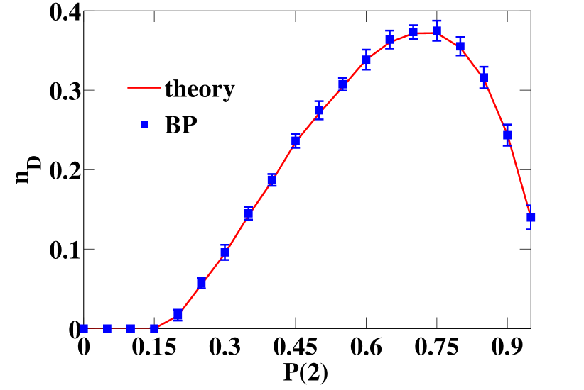
We consider a model of duplex network in which the replica nodes of the directed random graphs in the two layers have correlated degrees. In particular, we consider a case in which only the low in-degree nodes (nodes with in-degree equal to 0,1,20120,1,2) are correlated (replica nodes in different layers have same degree with probability p𝑝p) and a case in which the in-degrees of the replica nodes are equal with probability p𝑝p independently of their value (see Supplementary Material for details). The controllability of the network is affected by these correlations as shown in Figure 4. In fact, the number of driver nodes nDsubscript𝑛𝐷n_{D} decreases as the level of correlation increases. In duplex networks with Poisson degree distribution, low-degree correlations modify both the position of the hybrid transition and the size of the discontinuity. Once the replica nodes with low in-degree are correlated, a further correlation of the remaining replica nodes does not substantially change the number of driver nodes. This result confirms that structural controllability is essentially determined by the control of low degree nodes PRL .

Stability of the fully controllable solution –

A fully controllable solution, in which a single driver node is necessary to control the whole duplex network, exists if the minimum in-degree and the minimum out-degree are both greater than 111 in both layers. This solution of the cavity equations gives the correct solution to the maximum matching problem describing the controllability of multilayer networks only if no instabilities take place. The stability conditions are then found by imposing that the Jacobian of the systems of equations derived by the cavity method has all its eigenvalues λisubscript𝜆𝑖\lambda_{i} of modulus less than one, i.e. |λi|<1subscript𝜆𝑖1|\lambda_{i}|<1. In random duplex networks with the same degree distribution in the two layers, the fully controllable solution is stable (see Supplementary Material for the details of the derivation) if and only if

Pαout(2)<kαinkαout2kα(kα1)in,superscriptsubscript𝑃𝛼𝑜𝑢𝑡2subscriptdelimited-⟨⟩superscript𝑘𝛼𝑖𝑛subscriptdelimited-⟨⟩superscript𝑘𝛼𝑜𝑢𝑡2subscriptdelimited-⟨⟩superscript𝑘𝛼superscript𝑘𝛼1𝑖𝑛\displaystyle P_{\alpha}^{out}(2)<\frac{\langle{k^{\alpha}}\rangle_{in}\langle{k^{\alpha}}\rangle_{out}}{2\left\langle{k^{\alpha}(k^{\alpha}-1)}\right\rangle_{in}}, (10)

for α=A,B𝛼𝐴𝐵\alpha=A,B. On single networks it was instead recently found PRL that the fully controllable configuration is only stable for

Pin(2)<kin22k(k1)out,Pout(2)<kin22k(k1)in.formulae-sequencesuperscript𝑃𝑖𝑛2superscriptsubscriptdelimited-⟨⟩𝑘𝑖𝑛22subscriptdelimited-⟨⟩𝑘𝑘1𝑜𝑢𝑡superscript𝑃𝑜𝑢𝑡2subscriptsuperscriptdelimited-⟨⟩𝑘2𝑖𝑛2subscriptdelimited-⟨⟩𝑘𝑘1𝑖𝑛\displaystyle P^{in}(2)<\frac{\langle{k}\rangle_{in}^{2}}{2\left\langle{k(k-1)}\right\rangle_{out}},\ \ P^{out}(2)<\frac{\langle{k}\rangle^{2}_{in}}{2\left\langle{k(k-1)}\right\rangle_{in}}. (11)

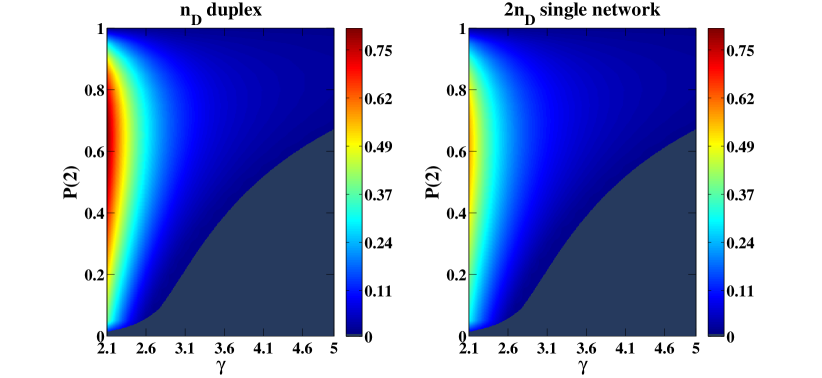
This implies that for multiplex networks with asymmetric in-degree and out-degree distributions it might occur that the fully controllable solution is stable in the multiplex network but unstable in the single networks taken in isolation (see Figure 5 for the characterization of the controllability of a similar type of multiplex networks). Therefore a multiplex structure can help to stabilize the fully controllable solution.

In conclusion, within the framework of structural controllability, we have considered the controllability properties of multiplex networks in which the nodes are either driver nodes in all the layers or they are not driver nodes in any layer. Our results show that controlling multiplex networks is more demanding, in terms of number of driver nodes, than controlling networks composed of a single layer. In random duplex networks with Poisson degree distribution, it is possible to observe a hybrid phase transition with a discontinuity in the number of driver nodes as a function of the average degree, that is phenomenologically similar to the emergence of mutually connected components. Close to this phase transition the duplex network exhibits an increased fragility to random damage. The existence of correlations between the degrees of replica nodes in different layers, in particular between low-degree nodes, has the effect of reducing the number of driver nodes necessary to control duplex networks. Finally, multiplex structure of networks can stabilize the fully controllable solution also if this solution is not stable in the single layers that form the multiplex network.

METHODS

The BP equations –

The BP equations of this problem are derived using the cavity method Mezard ; Cavity ; Weigt as described for the case of a single network problem in Lenka ; Altarelli ; Zecchina ; Liu ; PRL . The same approximation methods can be applied here, as long as the structure of the interconnected layers is locally tree-like both within the layers and across them. Under the decorrelation (replica-symmetric) assumption, the cavity fields (or messages) {hijα}superscriptsubscript𝑖𝑗𝛼\{h_{i\to j}^{\alpha}\} and {h^ijα}superscriptsubscript^𝑖𝑗𝛼\{\hat{h}_{i\to j}^{\alpha}\}, defined on the directed links between neighboring nodes (i,α)𝑖𝛼(i,\alpha) and (j,α)𝑗𝛼(j,\alpha) in the same layer α=A,B𝛼𝐴𝐵\alpha=A,B satisfy the zero-temperature limit of the BP equations, also known as Max-Sum equations,

hijαsuperscriptsubscript𝑖𝑗𝛼\displaystyle h_{i\to j}^{\alpha} =\displaystyle= max[1,maxk+ijh^kiα]1subscript𝑘superscript𝑖𝑗superscriptsubscript^𝑘𝑖𝛼\displaystyle-\max\left[-1,\max_{k\in\partial^{+}i\setminus j}\hat{h}_{k\to i}^{\alpha}\right]
h^ijAsubscriptsuperscript^𝐴𝑖𝑗\displaystyle\hat{h}^{A}_{i\to j} =\displaystyle= max[maxkAijhkiA,maxkBjhkiB]subscript𝑘superscriptsubscript𝐴𝑖𝑗superscriptsubscript𝑘𝑖𝐴subscript𝑘subscriptsuperscript𝐵𝑗superscriptsubscript𝑘𝑖𝐵\displaystyle-\max\left[\max_{k\in\partial_{-}^{A}i\setminus j}h_{k\to i}^{A},-\max_{k\in\partial^{B}_{-}j}h_{k\to i}^{B}\right]
h^ijBsubscriptsuperscript^𝐵𝑖𝑗\displaystyle\hat{h}^{B}_{i\to j} =\displaystyle= max[maxkBijhkiB,maxkAjhkiA]subscript𝑘superscriptsubscript𝐵𝑖𝑗superscriptsubscript𝑘𝑖𝐵subscript𝑘subscriptsuperscript𝐴𝑗superscriptsubscript𝑘𝑖𝐴\displaystyle-\max\left[\max_{k\in\partial_{-}^{B}i\setminus j}h_{k\to i}^{B},-\max_{k\in\partial^{A}_{-}j}h_{k\to i}^{A}\right] (12)

in which the fields are defined to take values in the discrete set {1,0,1}101\{-1,0,1\} and here and in the following we use the convention that the maximum over a null set is equal to 11-1 (see Supplementary Material for details). In terms of these fields, the energy E𝐸E in Eq.(9) becomes

E𝐸\displaystyle E =\displaystyle= αi=1Nmax[1,maxk+αih^kiα]+α(i,j)max[0,hijα+h^jiα]subscript𝛼superscriptsubscript𝑖1𝑁1subscript𝑘superscriptsubscript𝛼𝑖superscriptsubscript^𝑘𝑖𝛼subscript𝛼subscript𝑖𝑗0subscriptsuperscript𝛼𝑖𝑗subscriptsuperscript^𝛼𝑗𝑖\displaystyle-\sum_{\alpha}\sum_{i=1}^{N}\max\left[-1,\max_{k\in\partial_{+}^{\alpha}i}\hat{h}_{k\to i}^{\alpha}\right]+\sum_{\alpha}\sum_{(i,j)}\max\left[0,h^{\alpha}_{i\to j}+\hat{h}^{\alpha}_{j\to i}\right] (13)
i=1,Nmax[0,maxkAihkiA+maxkBihkiB].subscript𝑖1𝑁0subscript𝑘superscriptsubscript𝐴𝑖subscriptsuperscript𝐴𝑘𝑖subscript𝑘superscriptsubscript𝐵𝑖subscriptsuperscript𝐵𝑘𝑖\displaystyle-\sum_{i=1,N}\max\left[0,\max_{k\in\partial_{-}^{A}i}h^{A}_{k\to i}+\max_{k\in\partial_{-}^{B}i}h^{B}_{k\to i}\right].
BP equations over ensemble of networks-

Let us consider the case of uncorrelated duplex networks in which the degree of the same node in different layers are uncorrelated and there is no overlap of the links. In each layer α=A,B𝛼𝐴𝐵\alpha=A,B we consider a maximally random network with in-degree distribution Pα,in(k)superscript𝑃𝛼𝑖𝑛𝑘P^{\alpha,in}(k) and out-degree distribution Pα,out(k)superscript𝑃𝛼𝑜𝑢𝑡𝑘P^{\alpha,out}(k). At the ensemble level, each link of (the infinitely large) random network forming layer α𝛼\alpha has the same statistical properties, that we describe through distributions 𝒫α(hα)subscript𝒫𝛼superscript𝛼{\cal P}_{\alpha}(h^{\alpha}) and 𝒫^α(h^α)subscript^𝒫𝛼superscript^𝛼\hat{{\cal P}}_{\alpha}(\hat{h}^{\alpha}) of cavity fields that are defined on the support of Eqs. 12, i.e.

𝒫α(hα)subscript𝒫𝛼superscript𝛼\displaystyle{\cal P}_{\alpha}(h^{\alpha}) =\displaystyle= w1αδ(hα1)+w2αδ(hα+1)+w3αδ(hα),superscriptsubscript𝑤1𝛼𝛿superscript𝛼1superscriptsubscript𝑤2𝛼𝛿superscript𝛼1superscriptsubscript𝑤3𝛼𝛿superscript𝛼\displaystyle w_{1}^{\alpha}\delta(h^{\alpha}-1)+w_{2}^{\alpha}\delta(h^{\alpha}+1)+w_{3}^{\alpha}\delta(h^{\alpha}),
𝒫^α(h^α)subscript^𝒫𝛼superscript^𝛼\displaystyle\hat{{\cal P}}_{\alpha}(\hat{h}^{\alpha}) =\displaystyle= w^1αδ(h^α1)+w^2αδ(h^α+1)+w^3αδ(h^α),superscriptsubscript^𝑤1𝛼𝛿superscript^𝛼1superscriptsubscript^𝑤2𝛼𝛿superscript^𝛼1superscriptsubscript^𝑤3𝛼𝛿superscript^𝛼\displaystyle\hat{w}_{1}^{\alpha}\delta(\hat{h}^{\alpha}-1)+\hat{w}_{2}^{\alpha}\delta(\hat{h}^{\alpha}+1)+\hat{w}_{3}^{\alpha}\delta(\hat{h}^{\alpha}), (14)

where α=A,B𝛼𝐴𝐵\alpha=A,B and where the probabilities w1α,w2α,w3αsuperscriptsubscript𝑤1𝛼superscriptsubscript𝑤2𝛼superscriptsubscript𝑤3𝛼w_{1}^{\alpha},w_{2}^{\alpha},w_{3}^{\alpha} are normalized w1α+w2α+w3α=1superscriptsubscript𝑤1𝛼superscriptsubscript𝑤2𝛼superscriptsubscript𝑤3𝛼1w_{1}^{\alpha}+w_{2}^{\alpha}+w_{3}^{\alpha}=1 as well as the probabilities w^1α,w^2α,w^3αsuperscriptsubscript^𝑤1𝛼superscriptsubscript^𝑤2𝛼superscriptsubscript^𝑤3𝛼\hat{w}_{1}^{\alpha},\hat{w}_{2}^{\alpha},\hat{w}_{3}^{\alpha} that satisfy the equation w^1α+w^2α+w^3α=1superscriptsubscript^𝑤1𝛼superscriptsubscript^𝑤2𝛼superscriptsubscript^𝑤3𝛼1\hat{w}_{1}^{\alpha}+\hat{w}_{2}^{\alpha}+\hat{w}_{3}^{\alpha}=1. The cavity method at the network ensemble level is also known as density evolution method Mezard .

It is useful to introduce the generating functions G0α,in/out(z),superscriptsubscript𝐺0𝛼𝑖𝑛𝑜𝑢𝑡𝑧G_{0}^{\alpha,in/out}(z), and G1α,in/out(z)superscriptsubscript𝐺1𝛼𝑖𝑛𝑜𝑢𝑡𝑧G_{1}^{\alpha,in/out}(z) of the multiplex network as G0α,in/out(z)=kPα,in/out(k)zk,superscriptsubscript𝐺0𝛼𝑖𝑛𝑜𝑢𝑡𝑧subscript𝑘superscript𝑃𝛼𝑖𝑛𝑜𝑢𝑡𝑘superscript𝑧𝑘G_{0}^{\alpha,in/out}(z)=\sum_{k}P^{\alpha,in/out}(k)z^{k}, G1α,in/out(z)=kkkαPα,in/out(k)zk1,superscriptsubscript𝐺1𝛼𝑖𝑛𝑜𝑢𝑡𝑧subscript𝑘𝑘delimited-⟨⟩superscript𝑘𝛼superscript𝑃𝛼𝑖𝑛𝑜𝑢𝑡𝑘superscript𝑧𝑘1G_{1}^{\alpha,in/out}(z)=\sum_{k}\frac{k}{\langle{k^{\alpha}}\rangle}P^{\alpha,in/out}(k)z^{k-1}, with α=A,B𝛼𝐴𝐵\alpha=A,B. In this way, we can derive recursive equations for the probabilities {wiα}i=1,2,3subscriptsuperscriptsubscript𝑤𝑖𝛼𝑖123\{w_{i}^{\alpha}\}_{i=1,2,3} and {w^iα}i=1,2,3subscriptsuperscriptsubscript^𝑤𝑖𝛼𝑖123\{\hat{w}_{i}^{\alpha}\}_{i=1,2,3}, that are the analogous of the BP equations for an ensemble of uncorrelated duplex networks

w1αsuperscriptsubscript𝑤1𝛼\displaystyle w_{1}^{\alpha} =\displaystyle= G1α,out(w^2α),superscriptsubscript𝐺1𝛼𝑜𝑢𝑡superscriptsubscript^𝑤2𝛼\displaystyle G_{1}^{\alpha,out}(\hat{w}_{2}^{\alpha}),
w2αsuperscriptsubscript𝑤2𝛼\displaystyle w_{2}^{\alpha} =\displaystyle= [1G1α,out(1w^1α)],delimited-[]1superscriptsubscript𝐺1𝛼𝑜𝑢𝑡1superscriptsubscript^𝑤1𝛼\displaystyle\left[1-G_{1}^{\alpha,out}(1-\hat{w}_{1}^{\alpha})\right],
w^1Asuperscriptsubscript^𝑤1𝐴\displaystyle\hat{w}_{1}^{A} =\displaystyle= G1A,in(w2A)[1G0B,in(1w1B)],superscriptsubscript𝐺1𝐴𝑖𝑛superscriptsubscript𝑤2𝐴delimited-[]1superscriptsubscript𝐺0𝐵𝑖𝑛1superscriptsubscript𝑤1𝐵\displaystyle G_{1}^{A,in}(w_{2}^{A})\left[1-G_{0}^{B,in}(1-{w}_{1}^{B})\right],
w^2Asuperscriptsubscript^𝑤2𝐴\displaystyle\hat{w}_{2}^{A} =\displaystyle= [1G1A,in(1w1A)+G1A,in(1w1A)G0B,in(w2B)],delimited-[]1superscriptsubscript𝐺1𝐴𝑖𝑛1superscriptsubscript𝑤1𝐴superscriptsubscript𝐺1𝐴𝑖𝑛1superscriptsubscript𝑤1𝐴superscriptsubscript𝐺0𝐵𝑖𝑛superscriptsubscript𝑤2𝐵\displaystyle\left[1-G_{1}^{A,in}(1-w_{1}^{A})+G_{1}^{A,in}(1-w_{1}^{A})G_{0}^{B,in}\left(w_{2}^{B}\right)\right],
w^1Bsuperscriptsubscript^𝑤1𝐵\displaystyle\hat{w}_{1}^{B} =\displaystyle= G1B,in(w2B)[1G0A,in(1w1A)],superscriptsubscript𝐺1𝐵𝑖𝑛superscriptsubscript𝑤2𝐵delimited-[]1superscriptsubscript𝐺0𝐴𝑖𝑛1superscriptsubscript𝑤1𝐴\displaystyle G_{1}^{B,in}(w_{2}^{B})\left[1-G_{0}^{A,in}(1-{w}_{1}^{A})\right],
w^2Bsuperscriptsubscript^𝑤2𝐵\displaystyle\hat{w}_{2}^{B} =\displaystyle= [1G1B,in(1w1B)+G1B,in(1w1B)G0A,in(w2A)],delimited-[]1superscriptsubscript𝐺1𝐵𝑖𝑛1superscriptsubscript𝑤1𝐵superscriptsubscript𝐺1𝐵𝑖𝑛1superscriptsubscript𝑤1𝐵superscriptsubscript𝐺0𝐴𝑖𝑛superscriptsubscript𝑤2𝐴\displaystyle\left[1-G_{1}^{B,in}(1-w_{1}^{B})+G_{1}^{B,in}(1-w_{1}^{B})G_{0}^{A,in}\left(w_{2}^{A}\right)\right], (15)

with w3α=1w1αw2α,superscriptsubscript𝑤3𝛼1superscriptsubscript𝑤1𝛼superscriptsubscript𝑤2𝛼w_{3}^{\alpha}=1-w_{1}^{\alpha}-w_{2}^{\alpha}, and w^3α=1w^1αw^2αsuperscriptsubscript^𝑤3𝛼1superscriptsubscript^𝑤1𝛼superscriptsubscript^𝑤2𝛼\hat{w}_{3}^{\alpha}=1-\hat{w}_{1}^{\alpha}-\hat{w}_{2}^{\alpha}. The energy E𝐸E and the entropy density s𝑠s of the matching problem can be also expressed in terms of the {wiα}i=1,2,3subscriptsuperscriptsubscript𝑤𝑖𝛼𝑖123\{w_{i}^{\alpha}\}_{i=1,2,3} and {w^iα}i=1,2,3subscriptsuperscriptsubscript^𝑤𝑖𝛼𝑖123\{\hat{w}_{i}^{\alpha}\}_{i=1,2,3} (see Supplementary Material for details).

Hybrid transition for Poisson duplex network–

Here we consider the case of two Poisson networks with the same in/out average degree. In other words, we consider the situation in which kA,in=kA,out=kB,in=kB,out=cdelimited-⟨⟩superscript𝑘𝐴𝑖𝑛delimited-⟨⟩superscript𝑘𝐴𝑜𝑢𝑡delimited-⟨⟩superscript𝑘𝐵𝑖𝑛delimited-⟨⟩superscript𝑘𝐵𝑜𝑢𝑡𝑐\left\langle{k^{A,in}}\right\rangle=\left\langle{k^{A,out}}\right\rangle=\left\langle{k^{B,in}}\right\rangle=\left\langle{k^{B,out}}\right\rangle=c. We notice that the BP equations can be rewritten to form a closed subsystem of equations for w^1subscript^𝑤1\hat{w}_{1} and w^2subscript^𝑤2\hat{w}_{2} (see Supplementary Material for details),

w^1subscript^𝑤1\displaystyle\hat{w}_{1} =\displaystyle= h1(w^1,w^2)=ececw^1[1ecec(1w^2)]subscript1subscript^𝑤1subscript^𝑤2superscript𝑒𝑐superscript𝑒𝑐subscript^𝑤1delimited-[]1superscript𝑒𝑐superscript𝑒𝑐1subscript^𝑤2\displaystyle h_{1}(\hat{w}_{1},\hat{w}_{2})=e^{-ce^{-c\hat{w}_{1}}}\left[1-e^{-ce^{-c(1-\hat{w}_{2})}}\right] (16a)
w^2subscript^𝑤2\displaystyle\hat{w}_{2} =\displaystyle= h2(w^1,w^2)=[1ecec(1w^2)+ecec(1w^2)ececw^1]subscript2subscript^𝑤1subscript^𝑤2delimited-[]1superscript𝑒𝑐superscript𝑒𝑐1subscript^𝑤2superscript𝑒𝑐superscript𝑒𝑐1subscript^𝑤2superscript𝑒𝑐superscript𝑒𝑐subscript^𝑤1\displaystyle h_{2}(\hat{w}_{1},\hat{w}_{2})=\left[1-e^{-ce^{-c(1-\hat{w}_{2})}}+e^{-ce^{-c(1-\hat{w}_{2})}}e^{-ce^{-c\hat{w}_{1}}}\right] (16b)

from the solution of which the remaining quantities can be determined.

The value csuperscript𝑐c^{\star} of the average degree c𝑐c at which the discontinuity in the number of driver nodes nDsubscript𝑛𝐷n_{D} observed is found by imposing that Eqs. (16) are satisfied together with the condition

|J|=0,𝐽0\displaystyle\left|J\right|=0, (17)

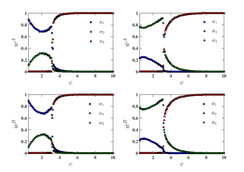
with J𝐽J indicating the Jacobian of the system of equations (16). Imposing that Eqs. (16) and condition (17) are simultaneously satisfied, the solution c=3.222326106superscript𝑐3.222326106c^{\star}=3.222326106\ldots is found. For c<c𝑐superscript𝑐c<c^{\star} we observe that w3=w^3=0subscript𝑤3subscript^𝑤30w_{3}=\hat{w}_{3}=0. At csuperscript𝑐c^{\star} we observe a discontinuity in both w3subscript𝑤3w_{3} and w^3subscript^𝑤3\hat{w}_{3}, but for c>c𝑐superscript𝑐c>c^{\star} the functions h1(w^1,w^2)subscript1subscript^𝑤1subscript^𝑤2h_{1}(\hat{w}_{1},\hat{w}_{2}) and h2(w^1,w^2)subscript2subscript^𝑤1subscript^𝑤2h_{2}(\hat{w}_{1},\hat{w}_{2}) are analytic, and analyzing Eqs. (16a)(16b)16a16b(\ref{2w1hatsameDN})-(\ref{2w2hatsameDN}) we obtain the behaviour of the order parameters w3subscript𝑤3w_{3} and w^3subscript^𝑤3\hat{w}_{3} for c>c𝑐superscript𝑐c>c^{\star}

w3w3subscript𝑤3superscriptsubscript𝑤3\displaystyle w_{3}-w_{3}^{\star} proportional-to\displaystyle\propto (cc)1/2superscript𝑐superscript𝑐12\displaystyle(c-c^{\star})^{1/2}
w^3w^3subscript^𝑤3superscriptsubscript^𝑤3\displaystyle\hat{w}_{3}-\hat{w}_{3}^{\star} proportional-to\displaystyle\propto (cc)1/2,superscript𝑐superscript𝑐12\displaystyle(c-c^{\star})^{1/2}, (18)

showing that the transition is hybrid.

Acknowledgements

LD aknowledges the European Research Council for grant n. 267915. GM aknowledges the European Project MIMOmics.

Author Contributions

GM, LD and GB designed the study, developed the methodology, performed the analysis and wrote the manuscript. The authors declare no competing financial interests.

Supplemental Material ”Control of Multilayer Networks”

.1 Introduction

This Supplemental Material is structured as follows.
In Sec. II we define the problem of structural controllability of multiplex networks, focusing on the case of a duplex network. Moreover we define the driver nodes, as the set of nodes that, if stimulated by an external signal, can drive the dynamical state of the network to any desired configuration.
In Sec. III we map the problem of structural controllability of a duplex network to a Maximum Matching Problem, and we derive the Belief Propagation (BP) equations determining the driver nodes, and their zero-temperature limit known as Max-Sum equations.
In Sec IV we consider the controllability of uncorrelated duplex networks, characterizing the BP equations valid for this problem, the stability conditions for the solutions of the BP equations, and the entropy of the solutions. Moreover, we consider duplex networks formed by two Poisson layers and we characterize their hybrid phase transition. Finally we consider the controllability of duplex networks formed by layers with power law in-degree and out-degree distributions.
In Sec. V we consider ensembles of duplex networks in which the in-degrees of replica nodes are correlated and we derive the BP equations assuming either that only the low in-degrees of replica nodes are correlated or that all the in-degrees of replica nodes are correlated.

.2 The structural controllability of a multiplex network

We consider a multiplex network in which every node i=1,2,,N𝑖12𝑁i=1,2,\ldots,N has a replica node in each layer and every layer is formed by a directed networks between the corresponding replica nodes PhysReports . We assume that each replica node can have a different dynamical state and can send different signals in the different networks (each layers is characterized by a different dynamical process). In this case the controllability of the multiplex network can be treated by control theory methods used for the single layers taken in isolation slotine ; Lin74 ; Liu ; PRL . Nevertheless here we will consider an additional constraint on the number of driver nodes. In fact we impose that corresponding replica nodes are either driver nodes in all layers or they are not driver nodes in any layer.

We consider for simplicity a duplex, i.e a multiplex formed by two layers where each layer is formed by a directed network. We call the two layers layer α=A,B𝛼𝐴𝐵\alpha=A,B. We consider a linear dynamical system determining the network dynamics

d𝐗(t)dt=𝒢𝐗(t)+𝒦𝐮(t),𝑑𝐗𝑡𝑑𝑡𝒢𝐗𝑡𝒦𝐮𝑡\displaystyle\frac{d{\bf X}(t)}{dt}={\cal G}{\bf X}(t)+{\cal K}{\bf u}(t), (19)

in which the vector 𝐗(t)𝐗𝑡{\bf X}(t) describes the dynamical state of each replica node in the duplex, and has 2N2𝑁2N elements. The first set of N𝑁N elements represents the dynamical state xiAsuperscriptsubscript𝑥𝑖𝐴x_{i}^{A} of node i𝑖i in layer A (i.e. Xi=xiAsubscript𝑋𝑖superscriptsubscript𝑥𝑖𝐴X_{i}=x_{i}^{A} for i=1,2,N𝑖12𝑁i=1,2\ldots,N), while the elements XN+isubscript𝑋𝑁𝑖X_{N+i} represent the dynamical state of the node i𝑖i in layer B, and are given by XN+i=xiBsubscript𝑋𝑁𝑖superscriptsubscript𝑥𝑖𝐵X_{N+i}=x_{i}^{B} for i=1,2,,N𝑖12𝑁i=1,2,\ldots,N. The matrix 𝒢𝒢{\cal G} is a 2N×2N2𝑁2𝑁2N\times 2N (asymmetric) matrix and the matrix 𝒦𝒦{\cal K} is a 2N×M2𝑁𝑀2N\times M matrix. The matrices 𝒢𝒢{\cal G} and 𝒦𝒦{\cal K} have the following block structure

𝒢=(gA00gB),𝒦=(KA00KB),formulae-sequence𝒢superscript𝑔𝐴0missing-subexpressionmissing-subexpression0superscript𝑔𝐵missing-subexpressionmissing-subexpression𝒦superscript𝐾𝐴00superscript𝐾𝐵\displaystyle{\cal G}=\left(\begin{array}[]{cccc}g^{A}&0\\ 0&g^{B}\end{array}\right),\ \ \ {\cal K}=\left(\begin{array}[]{cc}K^{A}&0\\ 0&K^{B}\end{array}\right), (24)

where gαsuperscript𝑔𝛼g^{\alpha} with α=A,B𝛼𝐴𝐵\alpha=A,B are the N×N𝑁𝑁N\times N matrices describing the directed weighted interactions within each of the networks in the two layers and Kαsuperscript𝐾𝛼{K}^{\alpha} are the N×Mα𝑁superscript𝑀𝛼N\times M^{\alpha} matrices describing the interaction between the nodes of the network α𝛼\alpha and the MαNsuperscript𝑀𝛼𝑁M^{\alpha}\leq N external signals for layer α𝛼\alpha. The external signals are indicated by the vector 𝐮(t)𝐮𝑡{\bf u}(t) of elements uγsubscript𝑢𝛾u_{\gamma} and γ=1,2M=MA+MBformulae-sequence𝛾12𝑀superscript𝑀𝐴superscript𝑀𝐵\gamma=1,2\ldots M=M^{A}+M^{B}.

Given block structure of both matrix 𝒢𝒢{\cal G} and 𝒦𝒦{\cal K} described in Eq. (24)24(\ref{bB}), the problem of duplex network controllability defined by Eq. (19)19(\ref{dyn}), can be exactly recast into the problem of controllability of the single layers that form the duplex network.

Here we adopt the framework of structural controllability Lin74 aimed at characterizing if a given duplex network is controllable when the non-zero matrix elements of 𝒢𝒢{\cal G} and 𝒦𝒦{\cal K} given by Eq. (24)24(\ref{bB}) are free parameters. A duplex networks in which the linear dynamics described by the Eqs. (19)19(\ref{dyn}) and (24)24(\ref{bB}) take place, is structurally controllable if both layers α=A,B𝛼𝐴𝐵\alpha=A,B are structurally controllable.

Each layer α𝛼\alpha is structurally controllable if for any choice of the free parameters in gαsuperscript𝑔𝛼{g^{\alpha}} and Kαsuperscript𝐾𝛼{K^{\alpha}}, except for a variety of zero Lebesgue measure in the parameter space, the Kalman’s condition is fulfilled Lin74 . Since structural controllability only distinguishes between zero and non-zero entries of the matrices gαsuperscript𝑔𝛼g^{\alpha} and Kαsuperscript𝐾𝛼{K^{\alpha}}, a given directed network in layer α𝛼\alpha is structurally controllable if it is possible to determine the input nodes (i.e. the position of the non-zero entries of the matrix Kαsuperscript𝐾𝛼{K^{\alpha}}) in a way to control the dynamics described by any realization of the matrix gαsuperscript𝑔𝛼{g^{\alpha}} with the same non-zero elements, except for atypical realizations of zero measure. In practice, a single network can be structurally controlled by identifying a minimum number of driver nodes, that are controlled nodes which do not share input vertices in both layers. In their seminal paper Liu , Liu and coworkers showed that on single networks this control theoretic problem can be reduced to a well-known optimization problem: their Minimum Input Theorem states that the minimum set of driver nodes that guarantees the full structural controllability of a network is the set of unmatched nodes in a maximum matching of the same directed network. Their result for a single network remains valid for the duplex network described by Eqs. (19)(24)1924(\ref{dyn})-(\ref{bB}). Therefore the structural controllability of duplex networks, in the absence of further constraints can be mapped to a Maximum Matching problem defined on the single layers of the duplex networks. Here nevertheless, we consider a further constraint to be imposed on the driver nodes, which enforce a new type of dependence between the layers of the duplex. In particular we impose that the replica nodes (i,α)𝑖𝛼(i,\alpha) with α=A,B𝛼𝐴𝐵\alpha=A,B and a given index i𝑖i, are either both driver nodes or neither is a driver node. This implies that these two replica nodes are either both linked to independent and external signals or none of them is connected to external signals.

.3 The Maximum Matching Problem for the Controllability of Duplex Networks

.3.1 Mapping duplex controllability into a constrained Maximum Matching Problem

In order to build an algorithm able to find the driver nodes of a duplex network we consider the variables sijα=1,0superscriptsubscript𝑠𝑖𝑗𝛼10s_{ij}^{\alpha}=1,0 indicating respectively if the directed link from node (i,α)𝑖𝛼(i,\alpha) to node (j,α)𝑗𝛼(j,\alpha) in layer α=A,B𝛼𝐴𝐵\alpha=A,B is matched or not. In the two layers of the duplex network we want to have a matching, i.e. the following constraints must always be satisfied for α=A,B𝛼𝐴𝐵\alpha=A,B,

j+αisijαsubscript𝑗superscriptsubscript𝛼𝑖superscriptsubscript𝑠𝑖𝑗𝛼\displaystyle\sum_{j\in\partial_{+}^{\alpha}i}s_{ij}^{\alpha} \displaystyle\leq 1,1\displaystyle 1, (25a)
jαisjiαsubscript𝑗superscriptsubscript𝛼𝑖superscriptsubscript𝑠𝑗𝑖𝛼\displaystyle\sum_{j\in\partial_{-}^{\alpha}i}s_{ji}^{\alpha} \displaystyle\leq 1,1\displaystyle 1, (25b)

where here and in the following we indicate with +αsuperscriptsubscript𝛼\partial_{+}^{\alpha} the set of nodes j𝑗j that are pointed by node i𝑖i in layer α𝛼\alpha and with αisuperscriptsubscript𝛼𝑖\partial_{-}^{\alpha}i the set of nodes j𝑗j pointing to node i𝑖i in layer α𝛼\alpha. In addition we impose that the driver nodes in the two networks are replica nodes, i.e. in the matching problem either two replica nodes are both matched or both unmatched. Therefore the variable sijαsuperscriptsubscript𝑠𝑖𝑗𝛼s_{ij}^{\alpha} satisfy the following additional constraints

iAjsjiA=iBjsjiB.subscript𝑖superscriptsubscript𝐴𝑗superscriptsubscript𝑠𝑗𝑖𝐴subscript𝑖superscriptsubscript𝐵𝑗superscriptsubscript𝑠𝑗𝑖𝐵\displaystyle\sum_{i\in\partial_{-}^{A}j}s_{ji}^{A}=\sum_{i\in\partial_{-}^{B}j}s_{ji}^{B}. (26)

Finally we need to minimize the number of driver nodes in the multiplex network. Therefore we minimize the energy E𝐸E of the problem given by

E𝐸\displaystyle E =\displaystyle= αj(1iαjsijα)=αiEiα,subscript𝛼subscript𝑗1subscript𝑖superscriptsubscript𝛼𝑗superscriptsubscript𝑠𝑖𝑗𝛼subscript𝛼subscript𝑖superscriptsubscript𝐸𝑖𝛼\displaystyle\sum_{\alpha}\sum_{j}\left(1-\sum_{i\in\partial_{-}^{\alpha}j}s_{ij}^{\alpha}\right)=\sum_{\alpha}\sum_{i}E_{i}^{\alpha}, (27)

with

Eiα=1j+αisijα.superscriptsubscript𝐸𝑖𝛼1subscript𝑗superscriptsubscript𝛼𝑖superscriptsubscript𝑠𝑖𝑗𝛼\displaystyle E_{i}^{\alpha}=1-\sum_{j\in\partial_{+}^{\alpha}i}s_{ij}^{\alpha}. (28)

The energy E𝐸E is given by the number NDsubscript𝑁𝐷N_{D} of driver replica nodes in the duplex network by

E=ND=NnD.𝐸subscript𝑁𝐷𝑁subscript𝑛𝐷\displaystyle E=N_{D}=Nn_{D}. (29)

.3.2 Derivation of the BP equations at finite inverse temperature β𝛽\beta

We consider here the Maximum Matching Problem defined in Sec .3.1. The goal is to find the configuration of the variables {sijα}superscriptsubscript𝑠𝑖𝑗𝛼\{s_{ij}^{\alpha}\} associated to every directed edge ij𝑖𝑗i\to j in layer α𝛼\alpha, such that the energy E𝐸E given by the number of driver replica nodes in the duplex network is minimized provided that the conditions given by Eqs. (25)25(\ref{uno}), (26)26(\ref{due}) are satisfied. Introducing as an auxiliary variable the “inverse temperature” β𝛽\beta we cast this problem into a statistical mechanics problem where our first aim is finding the distribution P({sij})𝑃subscript𝑠𝑖𝑗P(\{s_{ij}\}), parametrized by the inverse temperature β𝛽\beta, and given by

P({sij})𝑃subscript𝑠𝑖𝑗\displaystyle P(\{s_{ij}\}) =\displaystyle= eβEZi=1N{α[θ(1j+isijα)θ(1jisjiα)]δ(iAjsijA,iBjsijB)},superscript𝑒𝛽𝐸𝑍superscriptsubscriptproduct𝑖1𝑁subscriptproduct𝛼delimited-[]𝜃1subscript𝑗subscript𝑖superscriptsubscript𝑠𝑖𝑗𝛼𝜃1subscript𝑗subscript𝑖superscriptsubscript𝑠𝑗𝑖𝛼𝛿subscript𝑖superscriptsubscript𝐴𝑗superscriptsubscript𝑠𝑖𝑗𝐴subscript𝑖superscriptsubscript𝐵𝑗superscriptsubscript𝑠𝑖𝑗𝐵\displaystyle\frac{e^{-\beta E}}{Z}\prod_{i=1}^{N}\left\{\prod_{\alpha}\left[\theta\left(1-\sum_{j\in\partial_{+}i}s_{ij}^{\alpha}\right)\theta\left(1-\sum_{j\in\partial_{-}i}s_{ji}^{\alpha}\right)\right]\delta\left(\sum_{i\in\partial_{-}^{A}j}s_{ij}^{A},\sum_{i\in\partial_{-}^{B}j}s_{ij}^{B}\right)\right\}, (30)

where θ(x)=1𝜃𝑥1\theta(x)=1 for x0𝑥0x\geq 0 and θ(x)=0𝜃𝑥0\theta(x)=0 for x<0𝑥0x<0 , δ(x)𝛿𝑥\delta(x) is the Kronecker delta, and where Z𝑍Z is the normalization constant, that corresponds to the partition function of the statistical mechanics problem. Subsequently, we plan to perform the limit β𝛽\beta\to\infty in order to characterize the optimal (i.e. the maximum-sized) matching in the network satisfying Eqs. (25)25(\ref{uno}), (26)26(\ref{due}). The free-energy of the problem F(β)𝐹𝛽F(\beta) is defined as

βF(β)=lnZ,𝛽𝐹𝛽𝑍\displaystyle\beta F(\beta)=-\ln Z, (31)

and the energy E𝐸E is therefore given by

E=[βF(β)]β.𝐸delimited-[]𝛽𝐹𝛽𝛽\displaystyle E=\frac{\partial[\beta F(\beta)]}{\partial\beta}. (32)

The distribution P({sij})𝑃subscript𝑠𝑖𝑗P(\{s_{ij}\}) on a locally tree-like network can be (approximately) estimated by the cavity method in the replica symmetric assumption (i.e. by deriving Belief Propagation equations) Liu ; PRL ; Lenka ; Altarelli ; Mezard ; Cavity ; Zecchina ; Weigt . In this respect, in each layer α𝛼\alpha of the duplex network, we define two probability marginals on each directed link, one going in the same direction of the link Pijα(sij)superscriptsubscript𝑃𝑖𝑗𝛼subscript𝑠𝑖𝑗P_{i\to j}^{\alpha}(s_{ij}) and one in the opposite direction P^ijα(sji)superscriptsubscript^𝑃𝑖𝑗𝛼subscript𝑠𝑗𝑖\hat{P}_{i\to j}^{\alpha}(s_{ji}). The BP equations for these quantities are

Pijα(sij)superscriptsubscript𝑃𝑖𝑗𝛼subscript𝑠𝑖𝑗\displaystyle P_{i\to j}^{\alpha}(s_{ij}) =\displaystyle= 1𝒟ijα{sikα}|k+αij{θ(1k+αisikα)exp[β(1k+αisikα)]k+αijP^kiα(sikα)},1superscriptsubscript𝒟𝑖𝑗𝛼subscriptconditionalsuperscriptsubscript𝑠𝑖𝑘𝛼𝑘superscriptsubscript𝛼𝑖𝑗𝜃1subscript𝑘superscriptsubscript𝛼𝑖superscriptsubscript𝑠𝑖𝑘𝛼𝛽1subscript𝑘superscriptsubscript𝛼𝑖superscriptsubscript𝑠𝑖𝑘𝛼subscriptproduct𝑘superscriptsubscript𝛼𝑖𝑗superscriptsubscript^𝑃𝑘𝑖𝛼superscriptsubscript𝑠𝑖𝑘𝛼\displaystyle\frac{1}{{\cal D}_{i\to j}^{\alpha}}\sum_{\{s_{ik}^{\alpha}\}|k\in\partial_{+}^{\alpha}i\setminus j}\left\{\theta\left(1-\sum_{k\in\partial_{+}^{\alpha}i}s_{ik}^{\alpha}\right)\exp{\left[-\beta\left(1-\sum_{k\in\partial_{+}^{\alpha}i}s_{ik}^{\alpha}\right)\right]}\prod_{k\in\partial_{+}^{\alpha}i\setminus j}\hat{P}_{k\to i}^{\alpha}(s_{ik}^{\alpha})\right\}, (33a)
P^ijA(sjiA)superscriptsubscript^𝑃𝑖𝑗𝐴superscriptsubscript𝑠𝑗𝑖𝐴\displaystyle\hat{P}_{i\to j}^{A}(s_{ji}^{A}) =\displaystyle= 1𝒟^ijA{skiA}sjiA,kAi{θ(1kAiskiA){skiB}|kBi[θ(1kBiskiB)δ(iAjsijA,iBjsijB)\displaystyle\frac{1}{{\hat{\cal D}}_{i\to j}^{A}}\sum_{\{s_{ki}^{A}\}\setminus s_{ji}^{A},k\in\partial_{-}^{A}i}\left\{\theta\left(1-\sum_{k\in\partial_{-}^{A}i}s_{ki}^{A}\right)\sum_{\{s_{ki}^{B}\}|k\in\partial_{-}^{B}i}\left[\theta\left(1-\sum_{k\in\partial_{-}^{B}i}s_{ki}^{B}\right)\delta\left(\sum_{i\in\partial_{-}^{A}j}s_{ij}^{A},\sum_{i\in\partial_{-}^{B}j}s_{ij}^{B}\right)\right.\right. (33b)
×kAijPkiA(skiA)kBiPkiB(skiB)]},\displaystyle\times\left.\left.\prod_{k\in\partial_{-}^{A}i\setminus j}{P}_{k\to i}^{A}(s_{ki}^{A})\prod_{k\in\partial_{-}^{B}i}{P}_{k\to i}^{B}(s_{ki}^{B})\right]\right\},
P^ijB(sjiB)superscriptsubscript^𝑃𝑖𝑗𝐵superscriptsubscript𝑠𝑗𝑖𝐵\displaystyle\hat{P}_{i\to j}^{B}(s_{ji}^{B}) =\displaystyle= 1𝒟^ijB{skiB}|kBj{θ(1kBiskiB){skiA}|kAi[θ(1kAiskiA)δ(iAjsijA,iBjsijB)\displaystyle\frac{1}{{\hat{\cal D}}_{i\to j}^{B}}\sum_{\{s_{ki}^{B}\}|k\in\partial_{-}^{B}\setminus j}\left\{\theta\left(1-\sum_{k\in\partial_{-}^{B}i}s_{ki}^{B}\right)\sum_{\{s_{ki}^{A}\}|k\in\partial_{-}^{A}i}\left[\theta\left(1-\sum_{k\in\partial_{-}^{A}i}s_{ki}^{A}\right)\delta\left(\sum_{i\in\partial_{-}^{A}j}s_{ij}^{A},\sum_{i\in\partial_{-}^{B}j}s_{ij}^{B}\right)\right.\right. (33c)
×kBijPkiB(skiB)kAiPkiA(skiA)]}\displaystyle\times\left.\left.\prod_{k\in\partial_{-}^{B}i\setminus j}{P}_{k\to i}^{B}(s_{ki}^{B})\prod_{k\in\partial_{-}^{A}i}{P}_{k\to i}^{A}(s_{ki}^{A})\right]\right\}

where 𝒟ijαsuperscriptsubscript𝒟𝑖𝑗𝛼{\cal D}_{i\to j}^{\alpha} and 𝒟^ijαsuperscriptsubscript^𝒟𝑖𝑗𝛼{\hat{\cal D}}_{i\to j}^{\alpha} are normalization constants. The probability marginals {Pijα(sijα)\{P_{i\to j}^{\alpha}(s_{ij}^{\alpha}), P^ijα(sjiα)}\hat{P}_{i\to j}^{\alpha}(s_{ji}^{\alpha})\} can be parametrized by the cavity fields hijαsuperscriptsubscript𝑖𝑗𝛼h_{i\to j}^{\alpha} and h^ijαsuperscriptsubscript^𝑖𝑗𝛼\hat{h}_{i\to j}^{\alpha} defined by

Pijα(sijα)=exp[βhijαsijα]1+exp[βhijα]P^ijα(sjiα)=exp[βh^ijαsjiα]1+exp[βh^ijα].formulae-sequencesuperscriptsubscript𝑃𝑖𝑗𝛼superscriptsubscript𝑠𝑖𝑗𝛼𝛽superscriptsubscript𝑖𝑗𝛼superscriptsubscript𝑠𝑖𝑗𝛼1𝛽superscriptsubscript𝑖𝑗𝛼superscriptsubscript^𝑃𝑖𝑗𝛼superscriptsubscript𝑠𝑗𝑖𝛼𝛽superscriptsubscript^𝑖𝑗𝛼superscriptsubscript𝑠𝑗𝑖𝛼1𝛽superscriptsubscript^𝑖𝑗𝛼missing-subexpression\displaystyle\begin{array}[]{lr}P_{i\to j}^{\alpha}(s_{ij}^{\alpha})=\frac{\exp\left[{\beta h_{i\to j}^{\alpha}s_{ij}^{\alpha}}\right]}{1+\exp\left[{\beta h_{i\to j}^{\alpha}}\right]}\ \ \ \ \ \ \ \hat{P}_{i\to j}^{\alpha}(s_{ji}^{\alpha})=\frac{\exp\left[{\beta\hat{h}_{i\to j}^{\alpha}s_{ji}^{\alpha}}\right]}{1+\exp\left[{\beta\hat{h}_{i\to j}^{\alpha}}\right]}.&\end{array} (35)

In terms of the cavity fields (or messages), Eqs. (33) reduce to the following set of finite temperature BP equations,

hijαsuperscriptsubscript𝑖𝑗𝛼\displaystyle h_{i\to j}^{\alpha} =\displaystyle= 1βlog(eβ+k+αijeβh^kiα),1𝛽superscript𝑒𝛽subscript𝑘superscriptsubscript𝛼𝑖𝑗superscript𝑒𝛽superscriptsubscript^𝑘𝑖𝛼\displaystyle-\frac{1}{\beta}\log\left(e^{-\beta}+\sum_{k\in\partial_{+}^{\alpha}i\setminus j}e^{\beta\hat{h}_{k\to i}^{\alpha}}\right), (36a)
h^ijAsuperscriptsubscript^𝑖𝑗𝐴\displaystyle\hat{h}_{i\to j}^{A} =\displaystyle= 1βlog(1kBieβhkiB+kAijeβhkiA),1𝛽1subscript𝑘superscriptsubscript𝐵𝑖superscript𝑒𝛽superscriptsubscript𝑘𝑖𝐵subscript𝑘superscriptsubscript𝐴𝑖𝑗superscript𝑒𝛽subscriptsuperscript𝐴𝑘𝑖\displaystyle-\frac{1}{\beta}\log\left(\frac{1}{\sum_{k\in\partial_{-}^{B}i}e^{\beta h_{k\to i}^{B}}}+\sum_{k\in\partial_{-}^{A}i\setminus j}e^{\beta{h}^{A}_{k\to i}}\right), (36b)
h^ijBsuperscriptsubscript^𝑖𝑗𝐵\displaystyle\hat{h}_{i\to j}^{B} =\displaystyle= 1βlog(1kAieβhkjA+kBijeβhkiB),1𝛽1subscript𝑘superscriptsubscript𝐴𝑖superscript𝑒𝛽subscriptsuperscript𝐴𝑘𝑗subscript𝑘superscriptsubscript𝐵𝑖𝑗superscript𝑒𝛽subscriptsuperscript𝐵𝑘𝑖\displaystyle-\frac{1}{\beta}\log\left(\frac{1}{\sum_{k\in\partial_{-}^{A}i}e^{\beta h^{A}_{k\to j}}}+\sum_{k\in\partial_{-}^{B}i\setminus j}e^{\beta{h}^{B}_{k\to i}}\right), (36c)

The free energy F𝐹F and the energy E=βFβ𝐸𝛽𝐹𝛽E=\frac{\partial\beta F}{\partial\beta} of the model are given respectively by

βF𝛽𝐹\displaystyle-\beta F =\displaystyle= αi=1N[ln(eβ+k+αieβh^kiα)]+i=1,Nln(1+kAieβhkiAkBieβhkiB)subscript𝛼superscriptsubscript𝑖1𝑁delimited-[]superscript𝑒𝛽subscript𝑘superscriptsubscript𝛼𝑖superscript𝑒𝛽subscriptsuperscript^𝛼𝑘𝑖subscript𝑖1𝑁1subscript𝑘superscriptsubscript𝐴𝑖superscript𝑒𝛽superscriptsubscript𝑘𝑖𝐴subscriptsuperscript𝑘superscriptsubscript𝐵𝑖superscript𝑒𝛽superscriptsubscriptsuperscript𝑘𝑖𝐵\displaystyle\sum_{\alpha}\sum_{i=1}^{N}\left[\ln\left(e^{-\beta}+\sum_{k\in\partial_{+}^{\alpha}i}e^{\beta\hat{h}^{\alpha}_{k\to i}}\right)\right]+\sum_{i=1,N}\ln\left(1+\sum_{k\in\partial_{-}^{A}i}e^{\beta h_{k\to i}^{A}}\sum_{k^{\prime}\in\partial_{-}^{B}i}e^{\beta h_{k^{\prime}\to i}^{B}}\right) (37)
α<i,j>αln(1+eβ(hijα+h^jiα)),subscript𝛼subscriptabsent𝑖subscript𝛼𝑗absent1superscript𝑒𝛽superscriptsubscript𝑖𝑗𝛼superscriptsubscript^𝑗𝑖𝛼\displaystyle-\sum_{\alpha}\sum_{<i,j>_{\alpha}}\ln\left(1+e^{\beta(h_{i\to j}^{\alpha}+\hat{h}_{j\to i}^{\alpha})}\right),

and by

E𝐸\displaystyle E =\displaystyle= αi=1N[eβk+αih^kiαeβh^kiαeβ+k+αieβh^kiα]i=1NkAihkiAeβhkiAkBieβhkiB1+kAieβhkiAkBieβhkiBsubscript𝛼superscriptsubscript𝑖1𝑁delimited-[]superscript𝑒𝛽subscript𝑘superscriptsubscript𝛼𝑖subscriptsuperscript^𝛼𝑘𝑖superscript𝑒𝛽subscriptsuperscript^𝛼𝑘𝑖superscript𝑒𝛽subscript𝑘superscriptsubscript𝛼𝑖superscript𝑒𝛽subscriptsuperscript^𝛼𝑘𝑖superscriptsubscript𝑖1𝑁subscript𝑘superscriptsubscript𝐴𝑖superscriptsubscript𝑘𝑖𝐴superscript𝑒𝛽superscriptsubscript𝑘𝑖𝐴subscriptsuperscript𝑘superscriptsubscript𝐵𝑖superscript𝑒𝛽superscriptsubscriptsuperscript𝑘𝑖𝐵1subscript𝑘superscriptsubscript𝐴𝑖superscript𝑒𝛽superscriptsubscript𝑘𝑖𝐴subscriptsuperscript𝑘superscriptsubscript𝐵𝑖superscript𝑒𝛽superscriptsubscriptsuperscript𝑘𝑖𝐵\displaystyle\sum_{\alpha}\sum_{i=1}^{N}\left[\frac{e^{-\beta}-\sum_{k\in\partial_{+}^{\alpha}i}\hat{h}^{\alpha}_{k\to i}e^{\beta\hat{h}^{\alpha}_{k\to i}}}{e^{-\beta}+\sum_{k\in\partial_{+}^{\alpha}i}e^{\beta\hat{h}^{\alpha}_{k\to i}}}\right]-\sum_{i=1}^{N}\frac{\sum_{k\in\partial_{-}^{A}i}h_{k\to i}^{A}e^{\beta h_{k\to i}^{A}}\sum_{k^{\prime}\in\partial_{-}^{B}i}e^{\beta h_{k^{\prime}\to i}^{B}}}{1+\sum_{k\in\partial_{-}^{A}i}e^{\beta h_{k\to i}^{A}}\sum_{k^{\prime}\in\partial_{-}^{B}i}e^{\beta h_{k^{\prime}\to i}^{B}}} (38)
\displaystyle- ikAieβhkiAkBihkiBeβhkiB1+kAieβhkiAkBieβhkiB+α<i,j>α(hijα+h^jiα)eβ(hijα+h^jiα)1+eβ(hijα+h^jiα).subscript𝑖subscript𝑘superscriptsubscript𝐴𝑖superscript𝑒𝛽superscriptsubscript𝑘𝑖𝐴subscriptsuperscript𝑘superscriptsubscript𝐵𝑖superscriptsubscriptsuperscript𝑘𝑖𝐵superscript𝑒𝛽superscriptsubscriptsuperscript𝑘𝑖𝐵1subscript𝑘superscriptsubscript𝐴𝑖superscript𝑒𝛽superscriptsubscript𝑘𝑖𝐴subscriptsuperscript𝑘superscriptsubscript𝐵𝑖superscript𝑒𝛽superscriptsubscriptsuperscript𝑘𝑖𝐵subscript𝛼subscriptabsent𝑖subscript𝛼𝑗absentsuperscriptsubscript𝑖𝑗𝛼superscriptsubscript^𝑗𝑖𝛼superscript𝑒𝛽superscriptsubscript𝑖𝑗𝛼superscriptsubscript^𝑗𝑖𝛼1superscript𝑒𝛽superscriptsubscript𝑖𝑗𝛼superscriptsubscript^𝑗𝑖𝛼\displaystyle\sum_{i}\frac{\sum_{k\in\partial_{-}^{A}i}e^{\beta h_{k\to i}^{A}}\sum_{k^{\prime}\in\partial_{-}^{B}i}h_{k^{\prime}\to i}^{B}e^{\beta h_{k^{\prime}\to i}^{B}}}{1+\sum_{k\in\partial_{-}^{A}i}e^{\beta h_{k\to i}^{A}}\sum_{k^{\prime}\in\partial_{-}^{B}i}e^{\beta h_{k^{\prime}\to i}^{B}}}+\sum_{\alpha}\sum_{<i,j>_{\alpha}}\frac{(h_{i\to j}^{\alpha}+\hat{h}_{j\to i}^{\alpha})e^{\beta(h_{i\to j}^{\alpha}+\hat{h}_{j\to i}^{\alpha})}}{1+e^{\beta(h_{i\to j}^{\alpha}+\hat{h}_{j\to i}^{\alpha})}}.

.3.3 BP Equations for β𝛽\beta\to\infty

The BP equations in the limit β𝛽\beta\to\infty are derived from the Eqs. (36)36(\ref{BPbeta}). In the limit β𝛽\beta\to\infty the solution is expressed in terms of the fields hijαsuperscriptsubscript𝑖𝑗𝛼h_{i\to j}^{\alpha} or h^ijαsuperscriptsubscript^𝑖𝑗𝛼\hat{h}_{i\to j}^{\alpha} sent from a node (i,α)𝑖𝛼(i,\alpha) to the linked node (j,α)𝑗𝛼(j,\alpha) in layer α=A,B𝛼𝐴𝐵\alpha=A,B. The cavity fields have a simple interpretation as messages between neighboring replica nodes Lenka : hijα=h^ijα=1superscriptsubscript𝑖𝑗𝛼superscriptsubscript^𝑖𝑗𝛼1h_{i\to j}^{\alpha}=\hat{h}_{i\to j}^{\alpha}=1 means “match me”, hijα=h^ijα=1superscriptsubscript𝑖𝑗𝛼superscriptsubscript^𝑖𝑗𝛼1h_{i\to j}^{\alpha}=\hat{h}_{i\to j}^{\alpha}=-1 means “do not match me”, and hijα=h^ijα=0superscriptsubscript𝑖𝑗𝛼superscriptsubscript^𝑖𝑗𝛼0h_{i\to j}^{\alpha}=\hat{h}_{i\to j}^{\alpha}=0 means “do what you want”. The zero-temperature BP (or Max-Sum) equations determining the values of these fields in the limit β𝛽\beta\to\infty are are given by

hijαsuperscriptsubscript𝑖𝑗𝛼\displaystyle h_{i\to j}^{\alpha} =\displaystyle= max[1,maxk+ijh^kiα]1subscript𝑘superscript𝑖𝑗superscriptsubscript^𝑘𝑖𝛼\displaystyle-\max\left[-1,\max_{k\in\partial^{+}i\setminus j}\hat{h}_{k\to i}^{\alpha}\right] (39a)
h^ijAsubscriptsuperscript^𝐴𝑖𝑗\displaystyle\hat{h}^{A}_{i\to j} =\displaystyle= max[maxkAijhkiA,maxkBjhkiB]subscript𝑘superscriptsubscript𝐴𝑖𝑗superscriptsubscript𝑘𝑖𝐴subscript𝑘subscriptsuperscript𝐵𝑗superscriptsubscript𝑘𝑖𝐵\displaystyle-\max\left[\max_{k\in\partial_{-}^{A}i\setminus j}h_{k\to i}^{A},-\max_{k\in\partial^{B}_{-}j}h_{k\to i}^{B}\right] (39b)
h^ijBsubscriptsuperscript^𝐵𝑖𝑗\displaystyle\hat{h}^{B}_{i\to j} =\displaystyle= max[maxkBijhkiB,maxkAjhkiA]subscript𝑘superscriptsubscript𝐵𝑖𝑗superscriptsubscript𝑘𝑖𝐵subscript𝑘subscriptsuperscript𝐴𝑗superscriptsubscript𝑘𝑖𝐴\displaystyle-\max\left[\max_{k\in\partial_{-}^{B}i\setminus j}h_{k\to i}^{B},-\max_{k\in\partial^{A}_{-}j}h_{k\to i}^{A}\right] (39c)

in which the fields are defined to take values in the discrete set {1,0,1}101\{1,0,-1\} and we defined the maximum over a null set equal to 11-1. It follows that for kiB,in=0subscriptsuperscript𝑘𝐵𝑖𝑛𝑖0k^{{B},in}_{i}=0 we have h^ijA=1subscriptsuperscript^𝐴𝑖𝑗1\hat{h}^{A}_{i\to j}=-1 and for kiA,in=0subscriptsuperscript𝑘𝐴𝑖𝑛𝑖0k^{{A},in}_{i}=0 we have h^ijB=1subscriptsuperscript^𝐵𝑖𝑗1\hat{h}^{B}_{i\to j}=-1.

The energy E𝐸E can also be expressed in terms of these fields and is given by

E𝐸\displaystyle E =\displaystyle= αi=1Nmax[1,maxk+αih^kiα]subscript𝛼superscriptsubscript𝑖1𝑁1subscript𝑘superscriptsubscript𝛼𝑖superscriptsubscript^𝑘𝑖𝛼\displaystyle-\sum_{\alpha}\sum_{i=1}^{N}\max\left[-1,\max_{k\in\partial_{+}^{\alpha}i}\hat{h}_{k\to i}^{\alpha}\right] (40)
+α<i,j>max[0,hijα+h^jiα]subscript𝛼subscriptabsent𝑖𝑗absent0subscriptsuperscript𝛼𝑖𝑗subscriptsuperscript^𝛼𝑗𝑖\displaystyle+\sum_{\alpha}\sum_{<i,j>}\max\left[0,h^{\alpha}_{i\to j}+\hat{h}^{\alpha}_{j\to i}\right]
i=1,Nmax[0,maxkAihkiA+maxkBihkiB],subscript𝑖1𝑁0subscript𝑘superscriptsubscript𝐴𝑖subscriptsuperscript𝐴𝑘𝑖subscript𝑘superscriptsubscript𝐵𝑖subscriptsuperscript𝐵𝑘𝑖\displaystyle-\sum_{i=1,N}\max\left[0,\max_{k\in\partial_{-}^{A}i}h^{A}_{k\to i}+\max_{k\in\partial_{-}^{B}i}h^{B}_{k\to i}\right],

where <i,j><i,j> indicates pair of nodes that are nearest neighbors in the network and where we take the maximum over a null set equal to -1.

.4 Controllability of uncorrelated multiplex networks with given in-degree and out-degree distribution

.4.1 Cavity equations for an uncorrelated multiplex network ensemble

Let us consider the case of uncorrelated duplex networks in which the degree of the same node in different layers are uncorrelated and there is no overlap of the links. In each layer α=A,B𝛼𝐴𝐵\alpha=A,B we consider a maximally random network with in-degree distribution Pα,in(k)superscript𝑃𝛼𝑖𝑛𝑘P^{\alpha,in}(k) and out-degree distribution Pα,out(k)superscript𝑃𝛼𝑜𝑢𝑡𝑘P^{\alpha,out}(k). At the ensemble level, each link of (the infinitely large) random network forming layer α𝛼\alpha has the same statistical properties, that we describe through distributions 𝒫α(hα)subscript𝒫𝛼superscript𝛼{\cal P}_{\alpha}(h^{\alpha}) and 𝒫^α(h^α)subscript^𝒫𝛼superscript^𝛼\hat{{\cal P}}_{\alpha}(\hat{h}^{\alpha}) of cavity fields that are defined on the support of Eqs.39, i.e.

𝒫α(hα)subscript𝒫𝛼superscript𝛼\displaystyle{\cal P}_{\alpha}(h^{\alpha}) =\displaystyle= w1αδ(hα1)+w2αδ(hα+1)+w3αδ(hα),superscriptsubscript𝑤1𝛼𝛿superscript𝛼1superscriptsubscript𝑤2𝛼𝛿superscript𝛼1superscriptsubscript𝑤3𝛼𝛿superscript𝛼\displaystyle w_{1}^{\alpha}\delta(h^{\alpha}-1)+w_{2}^{\alpha}\delta(h^{\alpha}+1)+w_{3}^{\alpha}\delta(h^{\alpha}),
𝒫^α(h^α)subscript^𝒫𝛼superscript^𝛼\displaystyle\hat{{\cal P}}_{\alpha}(\hat{h}^{\alpha}) =\displaystyle= w^1αδ(h^α1)+w^2αδ(h^α+1)+w^3αδ(h^α),superscriptsubscript^𝑤1𝛼𝛿superscript^𝛼1superscriptsubscript^𝑤2𝛼𝛿superscript^𝛼1superscriptsubscript^𝑤3𝛼𝛿superscript^𝛼\displaystyle\hat{w}_{1}^{\alpha}\delta(\hat{h}^{\alpha}-1)+\hat{w}_{2}^{\alpha}\delta(\hat{h}^{\alpha}+1)+\hat{w}_{3}^{\alpha}\delta(\hat{h}^{\alpha}), (41)

where α=A,B𝛼𝐴𝐵\alpha=A,B and where the probabilities w1α,w2α,w3αsuperscriptsubscript𝑤1𝛼superscriptsubscript𝑤2𝛼superscriptsubscript𝑤3𝛼w_{1}^{\alpha},w_{2}^{\alpha},w_{3}^{\alpha} are normalized w1α+w2α+w3α=1superscriptsubscript𝑤1𝛼superscriptsubscript𝑤2𝛼superscriptsubscript𝑤3𝛼1w_{1}^{\alpha}+w_{2}^{\alpha}+w_{3}^{\alpha}=1 as well as the probabilities w^1α,w^2α,w^3αsuperscriptsubscript^𝑤1𝛼superscriptsubscript^𝑤2𝛼superscriptsubscript^𝑤3𝛼\hat{w}_{1}^{\alpha},\hat{w}_{2}^{\alpha},\hat{w}_{3}^{\alpha} that satisfy the equation w^1α+w^2α+w^3α=1superscriptsubscript^𝑤1𝛼superscriptsubscript^𝑤2𝛼superscriptsubscript^𝑤3𝛼1\hat{w}_{1}^{\alpha}+\hat{w}_{2}^{\alpha}+\hat{w}_{3}^{\alpha}=1. The cavity method at the network ensemble level is also known as density evolution method Mezard .

It is useful to introduce the generating functions G0α,in/out(z),superscriptsubscript𝐺0𝛼𝑖𝑛𝑜𝑢𝑡𝑧G_{0}^{\alpha,in/out}(z), and G1α,in/out(z)superscriptsubscript𝐺1𝛼𝑖𝑛𝑜𝑢𝑡𝑧G_{1}^{\alpha,in/out}(z) of the multiplex network as

G0α,in(z)superscriptsubscript𝐺0𝛼𝑖𝑛𝑧\displaystyle G_{0}^{\alpha,in}(z) =\displaystyle= kPα,in(k)zk,subscript𝑘superscript𝑃𝛼𝑖𝑛𝑘superscript𝑧𝑘\displaystyle\sum_{k}P^{\alpha,in}(k)z^{k},
G1α,in(z)superscriptsubscript𝐺1𝛼𝑖𝑛𝑧\displaystyle G_{1}^{\alpha,in}(z) =\displaystyle= kkkαPα,in(k)zk1,subscript𝑘𝑘delimited-⟨⟩superscript𝑘𝛼superscript𝑃𝛼𝑖𝑛𝑘superscript𝑧𝑘1\displaystyle\sum_{k}\frac{k}{\langle{k^{\alpha}}\rangle}P^{\alpha,in}(k)z^{k-1},
G0α,out(z)superscriptsubscript𝐺0𝛼𝑜𝑢𝑡𝑧\displaystyle G_{0}^{\alpha,out}(z) =\displaystyle= kPα,out(k)zk,subscript𝑘superscript𝑃𝛼𝑜𝑢𝑡𝑘superscript𝑧𝑘\displaystyle\sum_{k}P^{\alpha,out}(k)z^{k},
G1α,out(z)superscriptsubscript𝐺1𝛼𝑜𝑢𝑡𝑧\displaystyle G_{1}^{\alpha,out}(z) =\displaystyle= kkkαPα,out(k)zk1,subscript𝑘𝑘delimited-⟨⟩superscript𝑘𝛼superscript𝑃𝛼𝑜𝑢𝑡𝑘superscript𝑧𝑘1\displaystyle\sum_{k}\frac{k}{\langle{k^{\alpha}}\rangle}P^{\alpha,out}(k)z^{k-1}, (42)

with α=A,B𝛼𝐴𝐵\alpha=A,B. In this way, we can derive recursive equations for the probabilities {wiα}i=1,2,3subscriptsuperscriptsubscript𝑤𝑖𝛼𝑖123\{w_{i}^{\alpha}\}_{i=1,2,3} and {w^iα}i=1,2,3subscriptsuperscriptsubscript^𝑤𝑖𝛼𝑖123\{\hat{w}_{i}^{\alpha}\}_{i=1,2,3}, that are the analogous of Eqs. 39 for an ensemble of uncorrelated duplex networks

w1αsuperscriptsubscript𝑤1𝛼\displaystyle w_{1}^{\alpha} =\displaystyle= G1α,out(w^2α),superscriptsubscript𝐺1𝛼𝑜𝑢𝑡superscriptsubscript^𝑤2𝛼\displaystyle G_{1}^{\alpha,out}(\hat{w}_{2}^{\alpha}),
w2αsuperscriptsubscript𝑤2𝛼\displaystyle w_{2}^{\alpha} =\displaystyle= [1G1α,out(1w^1α)],delimited-[]1superscriptsubscript𝐺1𝛼𝑜𝑢𝑡1superscriptsubscript^𝑤1𝛼\displaystyle\left[1-G_{1}^{\alpha,out}(1-\hat{w}_{1}^{\alpha})\right],
w3αsuperscriptsubscript𝑤3𝛼\displaystyle w_{3}^{\alpha} =\displaystyle= 1w1αw2α,1superscriptsubscript𝑤1𝛼superscriptsubscript𝑤2𝛼\displaystyle 1-w_{1}^{\alpha}-w_{2}^{\alpha},
w^3αsuperscriptsubscript^𝑤3𝛼\displaystyle\hat{w}_{3}^{\alpha} =\displaystyle= 1w^1αw^2α,1superscriptsubscript^𝑤1𝛼superscriptsubscript^𝑤2𝛼\displaystyle 1-\hat{w}_{1}^{\alpha}-\hat{w}_{2}^{\alpha},
w^1Asuperscriptsubscript^𝑤1𝐴\displaystyle\hat{w}_{1}^{A} =\displaystyle= G1A,in(w2A)[1G0B,in(1w1B)],superscriptsubscript𝐺1𝐴𝑖𝑛superscriptsubscript𝑤2𝐴delimited-[]1superscriptsubscript𝐺0𝐵𝑖𝑛1superscriptsubscript𝑤1𝐵\displaystyle G_{1}^{A,in}(w_{2}^{A})\left[1-G_{0}^{B,in}(1-{w}_{1}^{B})\right],
w^2Asuperscriptsubscript^𝑤2𝐴\displaystyle\hat{w}_{2}^{A} =\displaystyle= [1G1A,in(1w1A)+G1A,in(1w1A)G0B,in(w2B)],delimited-[]1superscriptsubscript𝐺1𝐴𝑖𝑛1superscriptsubscript𝑤1𝐴superscriptsubscript𝐺1𝐴𝑖𝑛1superscriptsubscript𝑤1𝐴superscriptsubscript𝐺0𝐵𝑖𝑛superscriptsubscript𝑤2𝐵\displaystyle\left[1-G_{1}^{A,in}(1-w_{1}^{A})+G_{1}^{A,in}(1-w_{1}^{A})G_{0}^{B,in}\left(w_{2}^{B}\right)\right],
w^1Bsuperscriptsubscript^𝑤1𝐵\displaystyle\hat{w}_{1}^{B} =\displaystyle= G1B,in(w2B)[1G0A,in(1w1A)],superscriptsubscript𝐺1𝐵𝑖𝑛superscriptsubscript𝑤2𝐵delimited-[]1superscriptsubscript𝐺0𝐴𝑖𝑛1superscriptsubscript𝑤1𝐴\displaystyle G_{1}^{B,in}(w_{2}^{B})\left[1-G_{0}^{A,in}(1-{w}_{1}^{A})\right],
w^2Bsuperscriptsubscript^𝑤2𝐵\displaystyle\hat{w}_{2}^{B} =\displaystyle= [1G1B,in(1w1B)+G1B,in(1w1B)G0A,in(w2A)].delimited-[]1superscriptsubscript𝐺1𝐵𝑖𝑛1superscriptsubscript𝑤1𝐵superscriptsubscript𝐺1𝐵𝑖𝑛1superscriptsubscript𝑤1𝐵superscriptsubscript𝐺0𝐴𝑖𝑛superscriptsubscript𝑤2𝐴\displaystyle\left[1-G_{1}^{B,in}(1-w_{1}^{B})+G_{1}^{B,in}(1-w_{1}^{B})G_{0}^{A,in}\left(w_{2}^{A}\right)\right]. (43)

The energy E𝐸E of the matching problem can be also expressed in terms of the {wiα}i=1,2,3subscriptsuperscriptsubscript𝑤𝑖𝛼𝑖123\{w_{i}^{\alpha}\}_{i=1,2,3} and {w^iα}i=1,2,3subscriptsuperscriptsubscript^𝑤𝑖𝛼𝑖123\{\hat{w}_{i}^{\alpha}\}_{i=1,2,3} giving

E𝐸\displaystyle E =\displaystyle= α{G0α,out(w^2α)[1G0α,out(1w^1α)]}{[1G0A,in(1w1A)][1G0B,in(w2B)]\displaystyle\sum_{\alpha}\left\{G_{0}^{\alpha,out}\left(\hat{w}_{2}^{\alpha}\right)-\left[1-G_{0}^{\alpha,out}(1-\hat{w}_{1}^{\alpha})\right]\right\}-\left\{[1-G_{0}^{A,in}(1-w_{1}^{A})][1-G_{0}^{B,in}(w_{2}^{B})]\right. (44)
+[1G0B,in(1w1B)][1G0A,in(w2A)]}+αkαin[w^1α(1w2α)+w1α(1w^2α)].\displaystyle\left.+[1-G_{0}^{B,in}(1-w_{1}^{B})][1-G_{0}^{A,in}(w_{2}^{A})]\right\}+\sum_{\alpha}{\langle{k^{\alpha}}\rangle_{in}}\left[\hat{w}_{1}^{\alpha}(1-w_{2}^{\alpha})+w_{1}^{\alpha}(1-\hat{w}_{2}^{\alpha})\right].

.4.2 Stability condition

The Eqs.43 might have multiple solutions. In order to evaluate the stability of these solutions, using a method already used in the context of single networks PRL ; Lenka here we compute the Jacobian of the system of Eqs. (43) and impose that all its eigenvalues have modulus less than one. We avoid to consider w3αsuperscriptsubscript𝑤3𝛼w_{3}^{\alpha} and w^3αsuperscriptsubscript^𝑤3𝛼\hat{w}_{3}^{\alpha} because they influence only the number of null eigenvalues (4 eigenvalues upon 12). The 12×12121212\times 12 Jacobian matrix becomes 8×8888\times 8 and it can be decomposed in four 4×4444\times 4 blocks

J=(H11H1,2H2,1H2,2).𝐽subscript𝐻11subscript𝐻12subscript𝐻21subscript𝐻22\displaystyle J=\left(\begin{array}[]{cc}H_{11}&H_{1,2}\\ H_{2,1}&H_{2,2}\end{array}\right). (46)

with

H11=(000G2A,out(w^2A)00G2A,out(1w^1A)00G2A,in(w2A)(1G0B,in(1w1B))00G2A,in(1w1A)(1G0B,in(w2B))000),subscript𝐻11000superscriptsubscript𝐺2𝐴𝑜𝑢𝑡subscriptsuperscript^𝑤𝐴200superscriptsubscript𝐺2𝐴𝑜𝑢𝑡1subscriptsuperscript^𝑤𝐴100superscriptsubscript𝐺2𝐴𝑖𝑛subscriptsuperscript𝑤𝐴21superscriptsubscript𝐺0𝐵𝑖𝑛1superscriptsubscript𝑤1𝐵00superscriptsubscript𝐺2𝐴𝑖𝑛1superscriptsubscript𝑤1𝐴1superscriptsubscript𝐺0𝐵𝑖𝑛superscriptsubscript𝑤2𝐵000\displaystyle H_{11}=\left(\begin{array}[]{cccc}0&0&0&G_{2}^{A,out}(\hat{w}^{A}_{2})\\ 0&0&G_{2}^{A,out}(1-\hat{w}^{A}_{1})&0\\ 0&G_{2}^{A,in}(w^{A}_{2})(1-G_{0}^{B,in}(1-w_{1}^{B}))&0&0\\ G_{2}^{A,in}(1-w_{1}^{A})(1-G_{0}^{B,in}(w_{2}^{B}))&0&0&0\\ \end{array}\right), (51)
H2,1=(00000000G1B,in(w2B)kA,inG1A,in(1w1A)0000G1B,in(1w1B)kA,inG1A,in(w2A)00),subscript𝐻2100000000superscriptsubscript𝐺1𝐵𝑖𝑛subscriptsuperscript𝑤𝐵2subscriptdelimited-⟨⟩𝑘𝐴𝑖𝑛superscriptsubscript𝐺1𝐴𝑖𝑛1subscriptsuperscript𝑤𝐴10000superscriptsubscript𝐺1𝐵𝑖𝑛1subscriptsuperscript𝑤𝐵1subscriptdelimited-⟨⟩𝑘𝐴𝑖𝑛superscriptsubscript𝐺1𝐴𝑖𝑛subscriptsuperscript𝑤𝐴200\displaystyle H_{2,1}=\left(\begin{array}[]{cccc}0&0&0&0\\ 0&0&0&0\\ G_{1}^{B,in}(w^{B}_{2})\left\langle{k}\right\rangle_{A,in}G_{1}^{A,in}(1-w^{A}_{1})&0&0&0\\ 0&G_{1}^{B,in}(1-w^{B}_{1})\left\langle{k}\right\rangle_{A,in}G_{1}^{A,in}(w^{A}_{2})&0&0\end{array}\right), (56)
H1,2=(00000000G1A,in(w2A)kB,inG1B,in(1w1B)0000G1A,in(1w1A)kB,inG1B,in(w2B)00),subscript𝐻1200000000superscriptsubscript𝐺1𝐴𝑖𝑛subscriptsuperscript𝑤𝐴2subscriptdelimited-⟨⟩𝑘𝐵𝑖𝑛superscriptsubscript𝐺1𝐵𝑖𝑛1subscriptsuperscript𝑤𝐵10000superscriptsubscript𝐺1𝐴𝑖𝑛1subscriptsuperscript𝑤𝐴1subscriptdelimited-⟨⟩𝑘𝐵𝑖𝑛superscriptsubscript𝐺1𝐵𝑖𝑛subscriptsuperscript𝑤𝐵200\displaystyle H_{1,2}=\left(\begin{array}[]{cccc}0&0&0&0\\ 0&0&0&0\\ G_{1}^{A,in}(w^{A}_{2})\left\langle{k}\right\rangle_{B,in}G_{1}^{B,in}(1-w^{B}_{1})&0&0&0\\ 0&G_{1}^{A,in}(1-w^{A}_{1})\left\langle{k}\right\rangle_{B,in}G_{1}^{B,in}(w^{B}_{2})&0&0\end{array}\right), (61)

and

H2,2=(000G2B,out(w^2B)00G2B,out(1w^1B)00G2B,in(w2B)(1G0A,in(1w1A))00G2B,in(1w1B)(1G0A,in(w2A))000).subscript𝐻22000superscriptsubscript𝐺2𝐵𝑜𝑢𝑡subscriptsuperscript^𝑤𝐵200superscriptsubscript𝐺2𝐵𝑜𝑢𝑡1subscriptsuperscript^𝑤𝐵100superscriptsubscript𝐺2𝐵𝑖𝑛subscriptsuperscript𝑤𝐵21superscriptsubscript𝐺0𝐴𝑖𝑛1superscriptsubscript𝑤1𝐴00superscriptsubscript𝐺2𝐵𝑖𝑛1superscriptsubscript𝑤1𝐵1superscriptsubscript𝐺0𝐴𝑖𝑛superscriptsubscript𝑤2𝐴000\displaystyle H_{2,2}=\left(\begin{array}[]{cccc}0&0&0&G_{2}^{B,out}(\hat{w}^{B}_{2})\\ 0&0&G_{2}^{B,out}(1-\hat{w}^{B}_{1})&0\\ 0&G_{2}^{B,in}(w^{B}_{2})(1-G_{0}^{A,in}(1-w_{1}^{A}))&0&0\\ G_{2}^{B,in}(1-w_{1}^{B})(1-G_{0}^{A,in}(w_{2}^{A}))&0&0&0\\ \end{array}\right). (66)

Here the generating functions G0α,in/outsuperscriptsubscript𝐺0𝛼𝑖𝑛𝑜𝑢𝑡G_{0}^{\alpha,in/out} and G1α,in/outsuperscriptsubscript𝐺1𝛼𝑖𝑛𝑜𝑢𝑡G_{1}^{\alpha,in/out} are given by Eqs. (42)42(\ref{generating}) and the generating functions G2α,in(x)superscriptsubscript𝐺2𝛼𝑖𝑛𝑥G_{2}^{\alpha,in}(x) and G2α,out(x)superscriptsubscript𝐺2𝛼𝑜𝑢𝑡𝑥G_{2}^{\alpha,out}(x) are defined as

G2α,in(z)superscriptsubscript𝐺2𝛼𝑖𝑛𝑧\displaystyle G_{2}^{\alpha,in}(z) =\displaystyle= kk(k1)kαinPαin(k)zk2subscript𝑘𝑘𝑘1subscriptdelimited-⟨⟩superscript𝑘𝛼𝑖𝑛superscriptsubscript𝑃𝛼𝑖𝑛𝑘superscript𝑧𝑘2\displaystyle\sum_{k}\frac{k(k-1)}{\langle{k^{\alpha}}\rangle_{in}}P_{\alpha}^{in}(k)z^{k-2}
G2α,out(z)superscriptsubscript𝐺2𝛼𝑜𝑢𝑡𝑧\displaystyle G_{2}^{\alpha,out}(z) =\displaystyle= kk(k1)kαoutPαout(k)zk2.subscript𝑘𝑘𝑘1subscriptdelimited-⟨⟩superscript𝑘𝛼𝑜𝑢𝑡superscriptsubscript𝑃𝛼𝑜𝑢𝑡𝑘superscript𝑧𝑘2\displaystyle\sum_{k}\frac{k(k-1)}{\langle{k^{\alpha}}\rangle_{out}}P_{\alpha}^{out}(k)z^{k-2}. (67)

Of particular interest is the characterization of the stability of the solution w1α=w^1α=w2α=w^2α=0subscriptsuperscript𝑤𝛼1subscriptsuperscript^𝑤𝛼1subscriptsuperscript𝑤𝛼2subscriptsuperscript^𝑤𝛼20w^{\alpha}_{1}=\hat{w}^{\alpha}_{1}=w^{\alpha}_{2}=\hat{w}^{\alpha}_{2}=0 and w3α=w^3α=1superscriptsubscript𝑤3𝛼subscriptsuperscript^𝑤𝛼31w_{3}^{\alpha}=\hat{w}^{\alpha}_{3}=1, corresponding to the full controllability of the network, a configuration with E=ND=0𝐸subscript𝑁𝐷0E=N_{D}=0. This solution emerges for Pαin(1)=Pαout(1)=0superscriptsubscript𝑃𝛼𝑖𝑛1superscriptsubscript𝑃𝛼𝑜𝑢𝑡10P_{\alpha}^{in}(1)=P_{\alpha}^{out}(1)=0 for α=A,B𝛼𝐴𝐵\alpha=A,B. Therefore if the minimum in-degree and the minimum out-degree are both greater than one, the analysis at the ensemble level is consistent with the full controllability of the network. Nevertheless this solution might be not stable. By analyzing the Jacobian J𝐽J for w1α=w^1α=w2α=w^2α=0subscriptsuperscript𝑤𝛼1subscriptsuperscript^𝑤𝛼1subscriptsuperscript𝑤𝛼2subscriptsuperscript^𝑤𝛼20w^{\alpha}_{1}=\hat{w}^{\alpha}_{1}=w^{\alpha}_{2}=\hat{w}^{\alpha}_{2}=0 and w3α=w^3α=1superscriptsubscript𝑤3𝛼subscriptsuperscript^𝑤𝛼31w_{3}^{\alpha}=\hat{w}^{\alpha}_{3}=1, we can determine under which condition the full controllability solution is stable. The Jacobian matrix, in this case simplify significantly and is given by

J=(0002PAout(2)kAout000000kA(kA1)outkAout0000000000000kA(kA1)inkAin000000000000002PBout(2)kBout000000kB(kB1)outkBout0000000000000kB(kB1)inkBin000)𝐽0002superscriptsubscript𝑃𝐴𝑜𝑢𝑡2subscriptdelimited-⟨⟩superscript𝑘𝐴𝑜𝑢𝑡000000subscriptdelimited-⟨⟩superscript𝑘𝐴superscript𝑘𝐴1𝑜𝑢𝑡subscriptdelimited-⟨⟩superscript𝑘𝐴𝑜𝑢𝑡0000000000000subscriptdelimited-⟨⟩superscript𝑘𝐴superscript𝑘𝐴1𝑖𝑛subscriptdelimited-⟨⟩superscript𝑘𝐴𝑖𝑛000000000000002superscriptsubscript𝑃𝐵𝑜𝑢𝑡2subscriptdelimited-⟨⟩superscript𝑘𝐵𝑜𝑢𝑡000000subscriptdelimited-⟨⟩superscript𝑘𝐵superscript𝑘𝐵1𝑜𝑢𝑡subscriptdelimited-⟨⟩superscript𝑘𝐵𝑜𝑢𝑡0000000000000subscriptdelimited-⟨⟩superscript𝑘𝐵superscript𝑘𝐵1𝑖𝑛subscriptdelimited-⟨⟩superscript𝑘𝐵𝑖𝑛000J=\left(\begin{array}[]{cccccccc}0&0&0&\frac{2P_{A}^{out}(2)}{\langle{k^{A}}\rangle_{out}}&0&0&0&0\\ 0&0&\frac{\left\langle{k^{A}(k^{A}-1)}\right\rangle_{out}}{\langle{k^{A}}\rangle_{out}}&0&0&0&0&0\\ 0&0&0&0&0&0&0&0\\ \frac{\left\langle{k^{A}(k^{A}-1)}\right\rangle_{in}}{\langle{k^{A}}\rangle_{in}}&0&0&0&0&0&0&0\\ 0&0&0&0&0&0&0&\frac{2P_{B}^{out}(2)}{\langle{k^{B}}\rangle_{out}}\\ 0&0&0&0&0&0&\frac{\left\langle{k^{B}(k^{B}-1)}\right\rangle_{out}}{\langle{k^{B}}\rangle_{out}}&0\\ 0&0&0&0&0&0&0&0\\ 0&0&0&0&\frac{\left\langle{k^{B}(k^{B}-1)}\right\rangle_{in}}{\langle{k^{B}}\rangle_{in}}&0&0&0\\ \end{array}\right) (68)

Four eigenvalues of J𝐽J are zero, the other four have degenerate modulus, therefore the stability conditions are

2kA(kA1)inkAinPAout(2)kAout2subscriptdelimited-⟨⟩superscript𝑘𝐴superscript𝑘𝐴1𝑖𝑛subscriptdelimited-⟨⟩superscript𝑘𝐴𝑖𝑛superscriptsubscript𝑃𝐴𝑜𝑢𝑡2subscriptdelimited-⟨⟩superscript𝑘𝐴𝑜𝑢𝑡\displaystyle 2\frac{\left\langle{k^{A}(k^{A}-1)}\right\rangle_{in}}{\langle{k^{A}}\rangle_{in}}\frac{P_{A}^{out}(2)}{\langle{k^{A}}\rangle_{out}} <\displaystyle< 11\displaystyle 1
2kB(kB1)inkBinPBout(2)kBout2subscriptdelimited-⟨⟩superscript𝑘𝐵superscript𝑘𝐵1𝑖𝑛subscriptdelimited-⟨⟩superscript𝑘𝐵𝑖𝑛superscriptsubscript𝑃𝐵𝑜𝑢𝑡2subscriptdelimited-⟨⟩superscript𝑘𝐵𝑜𝑢𝑡\displaystyle 2\frac{\left\langle{k^{B}(k^{B}-1)}\right\rangle_{in}}{\langle{k^{B}}\rangle_{in}}\frac{P_{B}^{out}(2)}{\langle{k^{B}}\rangle_{out}} <\displaystyle< 1.1\displaystyle 1. (69)

When PAin(k)=PAout(k)=PBin(k)=PBout(k)=P(k)superscriptsubscript𝑃𝐴𝑖𝑛𝑘superscriptsubscript𝑃𝐴𝑜𝑢𝑡𝑘superscriptsubscript𝑃𝐵𝑖𝑛𝑘superscriptsubscript𝑃𝐵𝑜𝑢𝑡𝑘𝑃𝑘P_{A}^{in}(k)=P_{A}^{out}(k)=P_{B}^{in}(k)=P_{B}^{out}(k)=P(k) we have just one stability criterion solution and it reads

P(2)<k22k(k1)𝑃2superscriptdelimited-⟨⟩𝑘22delimited-⟨⟩𝑘𝑘1P(2)<\frac{\langle{k}\rangle^{2}}{2\left\langle{k(k-1)}\right\rangle} (70)

We observe here that on the single layers α=A,B𝛼𝐴𝐵\alpha=A,B the full controllability solution, is instead only stable PRL for

2kα(kα1)inkαinPαout(2)kαout2subscriptdelimited-⟨⟩superscript𝑘𝛼superscript𝑘𝛼1𝑖𝑛subscriptdelimited-⟨⟩superscript𝑘𝛼𝑖𝑛superscriptsubscript𝑃𝛼𝑜𝑢𝑡2subscriptdelimited-⟨⟩superscript𝑘𝛼𝑜𝑢𝑡\displaystyle 2\frac{\left\langle{k^{\alpha}(k^{\alpha}-1)}\right\rangle_{in}}{\langle{k^{\alpha}}\rangle_{in}}\frac{P_{\alpha}^{out}(2)}{\langle{k^{\alpha}}\rangle_{out}} <\displaystyle< 11\displaystyle 1
2kα(kα1)outkαoutPαin(2)kαin2subscriptdelimited-⟨⟩superscript𝑘𝛼superscript𝑘𝛼1𝑜𝑢𝑡subscriptdelimited-⟨⟩superscript𝑘𝛼𝑜𝑢𝑡superscriptsubscript𝑃𝛼𝑖𝑛2subscriptdelimited-⟨⟩superscript𝑘𝛼𝑖𝑛\displaystyle 2\frac{\left\langle{k^{\alpha}(k^{\alpha}-1)}\right\rangle_{out}}{\langle{k^{\alpha}}\rangle_{out}}\frac{P_{\alpha}^{in}(2)}{\langle{k^{\alpha}}\rangle_{in}} <\displaystyle< 1.1\displaystyle 1. (71)

It follows that for duplex networks in which both layers have the same in-degree and out-degree distributions, i.e. Pα,in(k)=Pα,out(k)superscript𝑃𝛼𝑖𝑛𝑘superscript𝑃𝛼𝑜𝑢𝑡𝑘P^{\alpha,in}(k)=P^{\alpha,out}(k) the stability of the full controllability solution on single layers is the same as the stability on the duplex network. Nevertheless, for duplex networks formed by layers in which the in-degree distribution and the out-degree distribution are not the same there can be cases in which for the duplex network the fully controllable solution is stable while for the single layers it is not stable (See main text for discussion of this phenomenon and simulation results).

.4.3 Entropy

In order to evaluate the number of maximum matchings, here we evaluate the entropy of the ground state solutions in the case of uncorrelated layers. The entropy density is given by s0=S0/Nsubscript𝑠0subscript𝑆0𝑁s_{0}=S_{0}/N and can be computed by expanding the free energy at low temperatures f(β)=e0s0/β+𝒪(1/β2)𝑓𝛽subscript𝑒0subscript𝑠0𝛽𝒪1superscript𝛽2f(\beta\to\infty)=e_{0}-s_{0}/\beta+{\cal O}(1/\beta^{2}). This involves the study of the evanescent parts of the cavity field. Therefore we assume that the field can be written as

hα=1+lnναβfor the peak around h=1hα=1+lnμαβfor the peak around h=1hα=lnγαβfor the peak around h=0subscript𝛼1subscript𝜈𝛼𝛽for the peak around 1subscript𝛼1subscript𝜇𝛼𝛽for the peak around 1subscript𝛼subscript𝛾𝛼𝛽for the peak around 0\displaystyle\begin{array}[]{ccc}h_{\alpha}=1+\frac{\ln\nu_{\alpha}}{\beta}&\mbox{for the peak around }&h=1\\ h_{\alpha}=-1+\frac{\ln\mu_{\alpha}}{\beta}&\mbox{for the peak around }&h=-1\\ h_{\alpha}=\frac{\ln\gamma_{\alpha}}{\beta}&\mbox{for the peak around }&h=0\\ \end{array}
h^α=1+lnν^αβfor the peak around h=1h^α=1+lnμ^αβfor the peak around h=1h^α=lnγ^αβfor the peak around h=0subscript^𝛼1subscript^𝜈𝛼𝛽for the peak around 1subscript^𝛼1subscript^𝜇𝛼𝛽for the peak around 1subscript^𝛼subscript^𝛾𝛼𝛽for the peak around 0\displaystyle\begin{array}[]{ccc}\hat{h}_{\alpha}=1+\frac{\ln\hat{\nu}_{\alpha}}{\beta}&\mbox{for the peak around }&h=1\\ \hat{h}_{\alpha}=-1+\frac{\ln\hat{\mu}_{\alpha}}{\beta}&\mbox{for the peak around }&h=-1\\ \hat{h}_{\alpha}=\frac{\ln\hat{\gamma}_{\alpha}}{\beta}&\mbox{for the peak around }&h=0\\ \end{array}

From the BP equations, and the equations for P(hα)𝑃subscript𝛼P(h_{\alpha}) and P(h^α)𝑃subscript^𝛼P(\hat{h}_{\alpha}) we can obtain the relation between the probability distributions 𝒜1α(να),𝒜2α(μα),𝒜3α(γα)superscriptsubscript𝒜1𝛼subscript𝜈𝛼superscriptsubscript𝒜2𝛼subscript𝜇𝛼superscriptsubscript𝒜3𝛼subscript𝛾𝛼{\cal A}_{1}^{\alpha}(\nu_{\alpha}),{\cal A}_{2}^{\alpha}(\mu_{\alpha}),{\cal A}_{3}^{\alpha}(\gamma_{\alpha}), and the distributions 𝒜^1α(ν^α),𝒜^2α(μα),𝒜^3α(γ^α)superscriptsubscript^𝒜1𝛼subscript^𝜈𝛼superscriptsubscript^𝒜2𝛼subscript𝜇𝛼superscriptsubscript^𝒜3𝛼subscript^𝛾𝛼\hat{{\cal A}}_{1}^{\alpha}(\hat{\nu}_{\alpha}),\hat{{\cal A}}_{2}^{\alpha}(\mu_{\alpha}),\hat{{\cal A}}_{3}^{\alpha}(\hat{\gamma}_{\alpha}), given by

𝒜1α(ν)superscriptsubscript𝒜1𝛼𝜈\displaystyle{\cal A}_{1}^{\alpha}(\nu) =\displaystyle= k=0(w^2α)kw1α(k+1)kαoutPoutα(k+1)[i=1kdμ^iα𝒜^2α(μ^iα)]δ(ν11+i=1kμ^iα)superscriptsubscript𝑘0superscriptsuperscriptsubscript^𝑤2𝛼𝑘superscriptsubscript𝑤1𝛼𝑘1delimited-⟨⟩subscriptsuperscript𝑘𝑜𝑢𝑡𝛼superscriptsubscript𝑃𝑜𝑢𝑡𝛼𝑘1delimited-[]superscriptsubscriptproduct𝑖1𝑘𝑑superscriptsubscript^𝜇𝑖𝛼superscriptsubscript^𝒜2𝛼superscriptsubscript^𝜇𝑖𝛼𝛿𝜈11superscriptsubscript𝑖1𝑘superscriptsubscript^𝜇𝑖𝛼\displaystyle\sum_{k=0}^{\infty}\frac{\left(\hat{w}_{2}^{\alpha}\right)^{k}}{w_{1}^{\alpha}}\frac{(k+1)}{\langle{k^{out}_{\alpha}}\rangle}P_{out}^{\alpha}(k+1)\int\left[\prod_{i=1}^{k}d{\hat{\mu}}_{i}^{\alpha}{\hat{\cal A}}_{2}^{\alpha}({\hat{\mu}}_{i}^{\alpha})\right]\delta\left(\nu-\frac{1}{1+\sum_{i=1}^{k}\hat{\mu}_{i}^{\alpha}}\right) (74)
𝒜2α(μ)superscriptsubscript𝒜2𝛼𝜇\displaystyle{\cal A}_{2}^{\alpha}(\mu) =\displaystyle= k=11w2αm=k(m+1)kαoutPoutα(m+1)(mk)(w^1α)k(1w^1α)mksuperscriptsubscript𝑘11superscriptsubscript𝑤2𝛼superscriptsubscript𝑚𝑘𝑚1delimited-⟨⟩subscriptsuperscript𝑘𝑜𝑢𝑡𝛼superscriptsubscript𝑃𝑜𝑢𝑡𝛼𝑚1binomial𝑚𝑘superscriptsuperscriptsubscript^𝑤1𝛼𝑘superscript1superscriptsubscript^𝑤1𝛼𝑚𝑘\displaystyle\sum_{k=1}^{\infty}\frac{1}{w_{2}^{\alpha}}\sum_{m=k}^{\infty}\frac{(m+1)}{\langle{k^{out}_{\alpha}}\rangle}P_{out}^{\alpha}(m+1)\binom{m}{k}(\hat{w}_{1}^{\alpha})^{k}(1-\hat{w}_{1}^{\alpha})^{m-k} (75)
×[i=1kdν^iα𝒜^1α(ν^iα)]δ(μ1i=1kν^iα)\displaystyle\times\int\left[\prod_{i=1}^{k}d{\hat{\nu}}_{i}^{\alpha}{\hat{\cal A}}_{1}^{\alpha}({\hat{\nu}}_{i}^{\alpha})\right]\delta\left(\mu-\frac{1}{\sum_{i=1}^{k}\hat{\nu}_{i}^{\alpha}}\right)
𝒜3α(γ)superscriptsubscript𝒜3𝛼𝛾\displaystyle{\cal A}_{3}^{\alpha}(\gamma) =\displaystyle= k=1m=k1w3α(m+1)kαoutPoutα(m+1)(mk)(w^3α)k(w^2α)mksuperscriptsubscript𝑘1superscriptsubscript𝑚𝑘1superscriptsubscript𝑤3𝛼𝑚1delimited-⟨⟩subscriptsuperscript𝑘𝑜𝑢𝑡𝛼superscriptsubscript𝑃𝑜𝑢𝑡𝛼𝑚1binomial𝑚𝑘superscriptsuperscriptsubscript^𝑤3𝛼𝑘superscriptsuperscriptsubscript^𝑤2𝛼𝑚𝑘\displaystyle\sum_{k=1}^{\infty}\sum_{m=k}^{\infty}\frac{1}{w_{3}^{\alpha}}\frac{(m+1)}{\langle{k^{out}_{\alpha}}\rangle}P_{out}^{\alpha}(m+1)\binom{m}{k}({\hat{w}}_{3}^{\alpha})^{k}(\hat{w}_{2}^{\alpha})^{m-k} (76)
×[i=1kdγ^iα𝒜^3α(γ^iα)]δ(γ1i=1kγ^iα)\displaystyle\times\int\left[\prod_{i=1}^{k}d\hat{\gamma}_{i}^{\alpha}{\hat{\cal A}}_{3}^{\alpha}(\hat{\gamma}_{i}^{\alpha})\right]\delta\left(\gamma-\frac{1}{\sum_{i=1}^{k}\hat{\gamma}_{i}^{\alpha}}\right)
𝒜^1A(ν^)superscriptsubscript^𝒜1𝐴^𝜈\displaystyle\hat{{\cal A}}_{1}^{A}(\hat{\nu}) =\displaystyle= kA=0(kA+1)kAinPinA(kA+1)(w2A)kAkB=1mB=kBPinB(mB)(mBkB)(w1B)kB(1w1B)mBkBsuperscriptsubscriptsuperscript𝑘𝐴0superscript𝑘𝐴1delimited-⟨⟩subscriptsuperscript𝑘𝑖𝑛𝐴superscriptsubscript𝑃𝑖𝑛𝐴superscript𝑘𝐴1superscriptsuperscriptsubscript𝑤2𝐴superscript𝑘𝐴superscriptsubscriptsuperscript𝑘𝐵1superscriptsubscriptsuperscript𝑚𝐵superscript𝑘𝐵superscriptsubscript𝑃𝑖𝑛𝐵superscript𝑚𝐵binomialsuperscript𝑚𝐵superscript𝑘𝐵superscriptsuperscriptsubscript𝑤1𝐵superscript𝑘𝐵superscript1superscriptsubscript𝑤1𝐵superscript𝑚𝐵superscript𝑘𝐵\displaystyle\sum_{k^{A}=0}^{\infty}\frac{(k^{A}+1)}{\langle{k^{in}_{A}}\rangle}P_{in}^{A}(k^{A}+1)(w_{2}^{A})^{k^{A}}\sum_{k^{B}=1}^{\infty}\sum_{m^{B}=k^{B}}^{\infty}P_{in}^{B}(m^{B})\binom{m^{B}}{k^{B}}(w_{1}^{B})^{k^{B}}(1-w_{1}^{B})^{m^{B}-k^{B}} (77)
[i=1kAdμiA𝒜2A(μiA)i=1kBdνiB𝒜1B(νiB)]×δ(ν^A11i=1kBνiB+i=1kAμiA)delimited-[]superscriptsubscriptproduct𝑖1superscript𝑘𝐴𝑑superscriptsubscript𝜇𝑖𝐴superscriptsubscript𝒜2𝐴superscriptsubscript𝜇𝑖𝐴superscriptsubscriptproduct𝑖1superscript𝑘𝐵𝑑superscriptsubscript𝜈𝑖𝐵superscriptsubscript𝒜1𝐵superscriptsubscript𝜈𝑖𝐵𝛿superscript^𝜈𝐴11superscriptsubscript𝑖1superscript𝑘𝐵superscriptsubscript𝜈𝑖𝐵superscriptsubscript𝑖1superscript𝑘𝐴superscriptsubscript𝜇𝑖𝐴\displaystyle\int\left[\prod_{i=1}^{k^{A}}d{\mu}_{i}^{A}{{\cal A}}_{2}^{A}({\mu}_{i}^{A})\prod_{i=1}^{k^{B}}d{\nu}_{i}^{B}{{\cal A}}_{1}^{B}({\nu}_{i}^{B})\right]\times\delta\left(\hat{\nu}^{A}-\frac{1}{\frac{1}{\sum_{i=1}^{k^{B}}\nu_{i}^{B}}+\sum_{i=1}^{k^{A}}{\mu}_{i}^{A}}\right)
𝒜^2A(μ^)superscriptsubscript^𝒜2𝐴^𝜇\displaystyle\hat{{\cal A}}_{2}^{A}(\hat{\mu}) =\displaystyle= 1w^2AG1A,in(1w1A)kBPinB(kB)(w2B)kB[i=1kBdμiB𝒜2B(μiB)]δ(μ^Ai=1kBμiB)1superscriptsubscript^𝑤2𝐴superscriptsubscript𝐺1𝐴𝑖𝑛1superscriptsubscript𝑤1𝐴subscriptsuperscript𝑘𝐵superscriptsubscript𝑃𝑖𝑛𝐵superscript𝑘𝐵superscriptsuperscriptsubscript𝑤2𝐵superscript𝑘𝐵delimited-[]superscriptsubscriptproduct𝑖1superscript𝑘𝐵𝑑superscriptsubscript𝜇𝑖𝐵superscriptsubscript𝒜2𝐵superscriptsubscript𝜇𝑖𝐵𝛿superscript^𝜇𝐴superscriptsubscript𝑖1superscript𝑘𝐵subscriptsuperscript𝜇𝐵𝑖\displaystyle\frac{1}{\hat{w}_{2}^{A}}G_{1}^{A,in}(1-w_{1}^{A})\sum_{k^{B}}P_{in}^{B}(k^{B})(w_{2}^{B})^{k^{B}}\int\left[\prod_{i=1}^{k^{B}}d{\mu}_{i}^{B}{{\cal A}}_{2}^{B}({\mu}_{i}^{B})\right]\delta\left(\hat{\mu}^{A}-\sum_{i=1}^{k^{B}}\mu^{B}_{i}\right) (78)
+\displaystyle+ 1w^2A(1G0B,in(w2B))kA=1mA=kA(m+1)kAinPinA(mA+1)(mAkA)(w1A)k(1w1A)mAkA1superscriptsubscript^𝑤2𝐴1superscriptsubscript𝐺0𝐵𝑖𝑛superscriptsubscript𝑤2𝐵superscriptsubscriptsuperscript𝑘𝐴1superscriptsubscriptsuperscript𝑚𝐴superscript𝑘𝐴𝑚1delimited-⟨⟩subscriptsuperscript𝑘𝑖𝑛𝐴superscriptsubscript𝑃𝑖𝑛𝐴superscript𝑚𝐴1binomialsuperscript𝑚𝐴superscript𝑘𝐴superscriptsuperscriptsubscript𝑤1𝐴𝑘superscript1superscriptsubscript𝑤1𝐴superscript𝑚𝐴superscript𝑘𝐴\displaystyle\frac{1}{\hat{w}_{2}^{A}}(1-G_{0}^{B,in}(w_{2}^{B}))\sum_{k^{A}=1}^{\infty}\sum_{m^{A}=k^{A}}^{\infty}\frac{(m+1)}{\langle{k^{in}_{A}}\rangle}P_{in}^{A}(m^{A}+1)\binom{m^{A}}{k^{A}}(w_{1}^{A})^{k}(1-w_{1}^{A})^{m^{A}-k^{A}}
×\displaystyle\times [i=1kAdνiA𝒜1(νiA)]δ(μ^A1i=1kAνiA)delimited-[]superscriptsubscriptproduct𝑖1superscript𝑘𝐴𝑑superscriptsubscript𝜈𝑖𝐴subscript𝒜1superscriptsubscript𝜈𝑖𝐴𝛿superscript^𝜇𝐴1superscriptsubscript𝑖1superscript𝑘𝐴superscriptsubscript𝜈𝑖𝐴\displaystyle\int\left[\prod_{i=1}^{k^{A}}d{\nu}_{i}^{A}{{\cal A}}_{1}({\nu}_{i}^{A})\right]\delta\left(\hat{\mu}^{A}-\frac{1}{\sum_{i=1}^{k^{A}}\nu_{i}^{A}}\right)
+\displaystyle+ 1w^2AkA=1mA=kA(m+1)kAinPinA(mA+1)(mAkA)(w1A)k(1w1A)mAkAkBPinB(kB)(w2B)kB1superscriptsubscript^𝑤2𝐴superscriptsubscriptsuperscript𝑘𝐴1superscriptsubscriptsuperscript𝑚𝐴superscript𝑘𝐴𝑚1delimited-⟨⟩subscriptsuperscript𝑘𝑖𝑛𝐴superscriptsubscript𝑃𝑖𝑛𝐴superscript𝑚𝐴1binomialsuperscript𝑚𝐴superscript𝑘𝐴superscriptsuperscriptsubscript𝑤1𝐴𝑘superscript1superscriptsubscript𝑤1𝐴superscript𝑚𝐴superscript𝑘𝐴subscriptsuperscript𝑘𝐵superscriptsubscript𝑃𝑖𝑛𝐵superscript𝑘𝐵superscriptsuperscriptsubscript𝑤2𝐵superscript𝑘𝐵\displaystyle\frac{1}{\hat{w}_{2}^{A}}\sum_{k^{A}=1}^{\infty}\sum_{m^{A}=k^{A}}^{\infty}\frac{(m+1)}{\langle{k^{in}_{A}}\rangle}P_{in}^{A}(m^{A}+1)\binom{m^{A}}{k^{A}}(w_{1}^{A})^{k}(1-w_{1}^{A})^{m^{A}-k^{A}}\sum_{k^{B}}P_{in}^{B}(k^{B})(w_{2}^{B})^{k^{B}}
×\displaystyle\times [i=1kAdνiA𝒜1A(νiA)i=1kBdμiB𝒜2B(μiB)]δ(μ^A11i=1kBμiB+i=1kAνiA)delimited-[]superscriptsubscriptproduct𝑖1superscript𝑘𝐴𝑑superscriptsubscript𝜈𝑖𝐴superscriptsubscript𝒜1𝐴superscriptsubscript𝜈𝑖𝐴superscriptsubscriptproduct𝑖1superscript𝑘𝐵𝑑superscriptsubscript𝜇𝑖𝐵superscriptsubscript𝒜2𝐵superscriptsubscript𝜇𝑖𝐵𝛿superscript^𝜇𝐴11superscriptsubscript𝑖1superscript𝑘𝐵superscriptsubscript𝜇𝑖𝐵superscriptsubscript𝑖1superscript𝑘𝐴superscriptsubscript𝜈𝑖𝐴\displaystyle\int\left[\prod_{i=1}^{k^{A}}d{\nu}_{i}^{A}{{\cal A}}_{1}^{A}({\nu}_{i}^{A})\prod_{i=1}^{k^{B}}d{\mu}_{i}^{B}{{\cal A}}_{2}^{B}({\mu}_{i}^{B})\right]\delta\left(\hat{\mu}^{A}-\frac{1}{\frac{1}{\sum_{i=1}^{k^{B}}\mu_{i}^{B}}+\sum_{i=1}^{k^{A}}\nu_{i}^{A}}\right)
𝒜^3A(γ^)superscriptsubscript^𝒜3𝐴^𝛾\displaystyle\hat{{\cal A}}_{3}^{A}(\hat{\gamma}) =\displaystyle= 1w^3AG1A,in(w2A)kB=1mB=kBPinB(kB)(mBkB)(w3B)k(w2B)mBkB1superscriptsubscript^𝑤3𝐴superscriptsubscript𝐺1𝐴𝑖𝑛superscriptsubscript𝑤2𝐴superscriptsubscriptsuperscript𝑘𝐵1superscriptsubscriptsuperscript𝑚𝐵superscript𝑘𝐵superscriptsubscript𝑃𝑖𝑛𝐵superscript𝑘𝐵binomialsuperscript𝑚𝐵superscript𝑘𝐵superscriptsuperscriptsubscript𝑤3𝐵𝑘superscriptsuperscriptsubscript𝑤2𝐵superscript𝑚𝐵superscript𝑘𝐵\displaystyle\frac{1}{\hat{w}_{3}^{A}}G_{1}^{A,in}(w_{2}^{A})\sum_{k^{B}=1}^{\infty}\sum_{m^{B}=k^{B}}^{\infty}P_{in}^{B}(k^{B})\binom{m^{B}}{k^{B}}(w_{3}^{B})^{k}(w_{2}^{B})^{m^{B}-k^{B}} (79)
×[i=1kBdγiB𝒜3B(γiB)]δ(γAi=1kBγiB)\displaystyle\times\int\left[\prod_{i=1}^{k^{B}}d{\gamma}_{i}^{B}{{\cal A}}_{3}^{B}({\gamma}_{i}^{B})\right]\delta\left(\gamma^{A}-\sum_{i=1}^{k_{B}}{\gamma}_{i}^{B}\right)
+\displaystyle+ 1w^3AkA=1mA=kA(mA+1)kAinPinA(mA+1)(mAkA)(w3A)k(w2A)mAkA1superscriptsubscript^𝑤3𝐴superscriptsubscriptsuperscript𝑘𝐴1superscriptsubscriptsuperscript𝑚𝐴superscript𝑘𝐴superscript𝑚𝐴1delimited-⟨⟩subscriptsuperscript𝑘𝑖𝑛𝐴superscriptsubscript𝑃𝑖𝑛𝐴superscript𝑚𝐴1binomialsuperscript𝑚𝐴superscript𝑘𝐴superscriptsuperscriptsubscript𝑤3𝐴𝑘superscriptsuperscriptsubscript𝑤2𝐴superscript𝑚𝐴superscript𝑘𝐴\displaystyle\frac{1}{\hat{w}_{3}^{A}}\sum_{k^{A}=1}^{\infty}\sum_{m^{A}=k^{A}}^{\infty}\frac{(m^{A}+1)}{\langle{k^{in}_{A}}\rangle}P_{in}^{A}(m^{A}+1)\binom{m^{A}}{k^{A}}(w_{3}^{A})^{k}(w_{2}^{A})^{m^{A}-k^{A}}
×\displaystyle\times kB=1mB=kBPinB(kB)(mBkB)(w3B)k(w2B)mBkB[i=1kAdγiA𝒜3A(γ^iA)i=1kBdγiB𝒜3B(γiB)]superscriptsubscriptsuperscript𝑘𝐵1superscriptsubscriptsuperscript𝑚𝐵superscript𝑘𝐵superscriptsubscript𝑃𝑖𝑛𝐵superscript𝑘𝐵binomialsuperscript𝑚𝐵superscript𝑘𝐵superscriptsuperscriptsubscript𝑤3𝐵𝑘superscriptsuperscriptsubscript𝑤2𝐵superscript𝑚𝐵superscript𝑘𝐵delimited-[]superscriptsubscriptproduct𝑖1superscript𝑘𝐴𝑑superscriptsubscript𝛾𝑖𝐴superscriptsubscript𝒜3𝐴superscriptsubscript^𝛾𝑖𝐴superscriptsubscriptproduct𝑖1superscript𝑘𝐵𝑑superscriptsubscript𝛾𝑖𝐵superscriptsubscript𝒜3𝐵superscriptsubscript𝛾𝑖𝐵\displaystyle\sum_{k^{B}=1}^{\infty}\sum_{m^{B}=k^{B}}^{\infty}P_{in}^{B}(k^{B})\binom{m^{B}}{k^{B}}(w_{3}^{B})^{k}(w_{2}^{B})^{m^{B}-k^{B}}\int\left[\prod_{i=1}^{k^{A}}d\gamma_{i}^{A}{\cal A}_{3}^{A}(\hat{\gamma}_{i}^{A})\prod_{i=1}^{k^{B}}d{\gamma}_{i}^{B}{{\cal A}}_{3}^{B}({\gamma}_{i}^{B})\right]
×\displaystyle\times δ(γA11i=1kBγiB+i=1kAγiA)𝛿superscript𝛾𝐴11superscriptsubscript𝑖1subscript𝑘𝐵superscriptsubscript𝛾𝑖𝐵superscriptsubscript𝑖1superscript𝑘𝐴superscriptsubscript𝛾𝑖𝐴\displaystyle\delta\left(\gamma^{A}-\frac{1}{\frac{1}{\sum_{i=1}^{k_{B}}{\gamma}_{i}^{B}}+\sum_{i=1}^{k^{A}}\gamma_{i}^{A}}\right)
+\displaystyle+ 1w^3A(1G0B,in(1w1B))kA=1mA=kA(mA+1)kAinPinA(mA+1)(mAkA)(w3A)k(w2A)mAkA1superscriptsubscript^𝑤3𝐴1superscriptsubscript𝐺0𝐵𝑖𝑛1superscriptsubscript𝑤1𝐵superscriptsubscriptsuperscript𝑘𝐴1superscriptsubscriptsuperscript𝑚𝐴superscript𝑘𝐴superscript𝑚𝐴1delimited-⟨⟩subscriptsuperscript𝑘𝑖𝑛𝐴superscriptsubscript𝑃𝑖𝑛𝐴superscript𝑚𝐴1binomialsuperscript𝑚𝐴superscript𝑘𝐴superscriptsuperscriptsubscript𝑤3𝐴𝑘superscriptsuperscriptsubscript𝑤2𝐴superscript𝑚𝐴superscript𝑘𝐴\displaystyle\frac{1}{\hat{w}_{3}^{A}}(1-G_{0}^{B,in}(1-w_{1}^{B}))\sum_{k^{A}=1}^{\infty}\sum_{m^{A}=k^{A}}^{\infty}\frac{(m^{A}+1)}{\langle{k^{in}_{A}}\rangle}P_{in}^{A}(m^{A}+1)\binom{m^{A}}{k^{A}}(w_{3}^{A})^{k}(w_{2}^{A})^{m^{A}-k^{A}}
×\displaystyle\times [i=1kAdγiA𝒜3A(γ^iA)]δ(γA1i=1kAγiA)delimited-[]superscriptsubscriptproduct𝑖1superscript𝑘𝐴𝑑superscriptsubscript𝛾𝑖𝐴superscriptsubscript𝒜3𝐴superscriptsubscript^𝛾𝑖𝐴𝛿superscript𝛾𝐴1superscriptsubscript𝑖1superscript𝑘𝐴superscriptsubscript𝛾𝑖𝐴\displaystyle\int\left[\prod_{i=1}^{k^{A}}d\gamma_{i}^{A}{\cal A}_{3}^{A}(\hat{\gamma}_{i}^{A})\right]\delta\left(\gamma^{A}-\frac{1}{\sum_{i=1}^{k^{A}}\gamma_{i}^{A}}\right)

The free energy density f(β)=F(β)/N=e0s0β+𝒪(1/β2)𝑓𝛽𝐹𝛽𝑁subscript𝑒0subscript𝑠0𝛽𝒪1superscript𝛽2f(\beta)=F(\beta)/N=e_{0}-\frac{s_{0}}{\beta}+{\cal O}(1/\beta^{2}) with

s0=s0,a,A+s0,a,B+s0,b+s0,c,A+s0,c,Bsubscript𝑠0subscript𝑠0𝑎𝐴subscript𝑠0𝑎𝐵subscript𝑠0𝑏subscript𝑠0𝑐𝐴subscript𝑠0𝑐𝐵s_{0}=s_{0,a,A}+s_{0,a,B}+s_{0,b}+s_{0,c,A}+s_{0,c,B} (80)

where s0,subscript𝑠0s_{0,\ell} are given by

s0,a,αsubscript𝑠0𝑎𝛼\displaystyle s_{0,a,\alpha} =\displaystyle= k=1m=k(mk)(w^1α)k(1(w^1α))mkPoutα(m)lni=1kν^i¯superscriptsubscript𝑘1superscriptsubscript𝑚𝑘binomial𝑚𝑘superscriptsuperscriptsubscript^𝑤1𝛼𝑘superscript1superscriptsubscript^𝑤1𝛼𝑚𝑘subscriptsuperscript𝑃𝛼𝑜𝑢𝑡𝑚¯superscriptsubscript𝑖1𝑘subscript^𝜈𝑖\displaystyle\sum_{k=1}^{\infty}\sum_{m=k}^{\infty}\binom{m}{k}(\hat{w}_{1}^{\alpha})^{k}(1-(\hat{w}_{1}^{\alpha}))^{m-k}P^{\alpha}_{out}(m)\overline{\ln\sum_{i=1}^{k}\hat{\nu}_{i}} (81)
+\displaystyle+ kPoutα(k)(w^2α)kln(1+i=1kμ^i)¯subscript𝑘subscriptsuperscript𝑃𝛼𝑜𝑢𝑡𝑘superscriptsuperscriptsubscript^𝑤2𝛼𝑘¯1superscriptsubscript𝑖1𝑘subscript^𝜇𝑖\displaystyle\sum_{k}P^{\alpha}_{out}(k)(\hat{w}_{2}^{\alpha})^{k}\overline{\ln\left(1+\sum_{i=1}^{k}\hat{\mu}_{i}\right)}
+\displaystyle+ k=1m=k(mk)(w^3α)k(w^2α)mkPoutα(m)ln(i=1kγ^i)¯superscriptsubscript𝑘1superscriptsubscript𝑚𝑘binomial𝑚𝑘superscriptsuperscriptsubscript^𝑤3𝛼𝑘superscriptsuperscriptsubscript^𝑤2𝛼𝑚𝑘subscriptsuperscript𝑃𝛼𝑜𝑢𝑡𝑚¯superscriptsubscript𝑖1𝑘subscript^𝛾𝑖\displaystyle\sum_{k=1}^{\infty}\sum_{m=k}^{\infty}\binom{m}{k}(\hat{w}_{3}^{\alpha})^{k}(\hat{w}_{2}^{\alpha})^{m-k}P^{\alpha}_{out}(m)\overline{\ln\left(\sum_{i=1}^{k}\hat{\gamma}_{i}\right)}
s0,bsubscript𝑠0𝑏\displaystyle s_{0,b} =\displaystyle= (1G0B,in(w2B))kA=1mA=kA(mAkA)(w1A)kA(1(w1A))mAkAPinA(mA)lni=1kAνiA¯1superscriptsubscript𝐺0𝐵𝑖𝑛superscriptsubscript𝑤2𝐵superscriptsubscriptsuperscript𝑘𝐴1superscriptsubscriptsuperscript𝑚𝐴superscript𝑘𝐴binomialsuperscript𝑚𝐴superscript𝑘𝐴superscriptsuperscriptsubscript𝑤1𝐴superscript𝑘𝐴superscript1superscriptsubscript𝑤1𝐴superscript𝑚𝐴superscript𝑘𝐴subscriptsuperscript𝑃𝐴𝑖𝑛superscript𝑚𝐴¯superscriptsubscript𝑖1superscript𝑘𝐴subscriptsuperscript𝜈𝐴𝑖\displaystyle(1-G_{0}^{B,in}(w_{2}^{B}))\sum_{k^{A}=1}^{\infty}\sum_{m^{A}=k^{A}}^{\infty}\binom{m^{A}}{k^{A}}(w_{1}^{A})^{k^{A}}(1-(w_{1}^{A}))^{m^{A}-k^{A}}P^{A}_{in}(m^{A})\overline{\ln\sum_{i=1}^{k^{A}}\nu^{A}_{i}} (82)
+\displaystyle+ (1G0A,in(w2A))kB=1mB=kB(mBkB)(w1B)kB(1(w1B))mBkBPinB(mB)lni=1kBνiB¯1superscriptsubscript𝐺0𝐴𝑖𝑛superscriptsubscript𝑤2𝐴superscriptsubscriptsuperscript𝑘𝐵1superscriptsubscriptsuperscript𝑚𝐵superscript𝑘𝐵binomialsuperscript𝑚𝐵superscript𝑘𝐵superscriptsuperscriptsubscript𝑤1𝐵superscript𝑘𝐵superscript1superscriptsubscript𝑤1𝐵superscript𝑚𝐵superscript𝑘𝐵subscriptsuperscript𝑃𝐵𝑖𝑛superscript𝑚𝐵¯superscriptsubscript𝑖1superscript𝑘𝐵subscriptsuperscript𝜈𝐵𝑖\displaystyle(1-G_{0}^{A,in}(w_{2}^{A}))\sum_{k^{B}=1}^{\infty}\sum_{m^{B}=k^{B}}^{\infty}\binom{m^{B}}{k^{B}}(w_{1}^{B})^{k^{B}}(1-(w_{1}^{B}))^{m^{B}-k^{B}}P^{B}_{in}(m^{B})\overline{\ln\sum_{i=1}^{k^{B}}\nu^{B}_{i}}
+\displaystyle+ (1G0B,in(1w1B))kA=1mA=kA(mAkA)(w3A)kA(w2A)mAkAPinA(mA)lni=1kAγiA¯1superscriptsubscript𝐺0𝐵𝑖𝑛1superscriptsubscript𝑤1𝐵superscriptsubscriptsuperscript𝑘𝐴1superscriptsubscriptsuperscript𝑚𝐴superscript𝑘𝐴binomialsuperscript𝑚𝐴superscript𝑘𝐴superscriptsuperscriptsubscript𝑤3𝐴superscript𝑘𝐴superscriptsuperscriptsubscript𝑤2𝐴superscript𝑚𝐴superscript𝑘𝐴subscriptsuperscript𝑃𝐴𝑖𝑛superscript𝑚𝐴¯superscriptsubscript𝑖1superscript𝑘𝐴subscriptsuperscript𝛾𝐴𝑖\displaystyle(1-G_{0}^{B,in}(1-w_{1}^{B}))\sum_{k^{A}=1}^{\infty}\sum_{m^{A}=k^{A}}^{\infty}\binom{m^{A}}{k^{A}}(w_{3}^{A})^{k^{A}}(w_{2}^{A})^{m^{A}-k^{A}}P^{A}_{in}(m^{A})\overline{\ln\sum_{i=1}^{k^{A}}\gamma^{A}_{i}}
+\displaystyle+ (1G0A,in(1w1A))kB=1mB=kB(mBkB)(w3B)kB(w2B)mBkBPinB(mB)lni=1kBγiB¯1superscriptsubscript𝐺0𝐴𝑖𝑛1superscriptsubscript𝑤1𝐴superscriptsubscriptsuperscript𝑘𝐵1superscriptsubscriptsuperscript𝑚𝐵superscript𝑘𝐵binomialsuperscript𝑚𝐵superscript𝑘𝐵superscriptsuperscriptsubscript𝑤3𝐵superscript𝑘𝐵superscriptsuperscriptsubscript𝑤2𝐵superscript𝑚𝐵superscript𝑘𝐵subscriptsuperscript𝑃𝐵𝑖𝑛superscript𝑚𝐵¯superscriptsubscript𝑖1superscript𝑘𝐵subscriptsuperscript𝛾𝐵𝑖\displaystyle(1-G_{0}^{A,in}(1-w_{1}^{A}))\sum_{k^{B}=1}^{\infty}\sum_{m^{B}=k^{B}}^{\infty}\binom{m^{B}}{k^{B}}(w_{3}^{B})^{k^{B}}(w_{2}^{B})^{m^{B}-k^{B}}P^{B}_{in}(m^{B})\overline{\ln\sum_{i=1}^{k^{B}}\gamma^{B}_{i}}
+\displaystyle+ [kBPinB(kB)(w2B)kBkA=1mA=kA(mAkA)(w1A)kA(1(w1A))mAkAPinA(mA)\displaystyle\left[\sum_{k^{B}}P^{B}_{in}(k^{B})(w_{2}^{B})^{k^{B}}\sum_{k^{A}=1}^{\infty}\sum_{m^{A}=k^{A}}^{\infty}\binom{m^{A}}{k^{A}}(w_{1}^{A})^{k^{A}}(1-(w_{1}^{A}))^{m^{A}-k^{A}}P^{A}_{in}(m^{A})\right.
×ln(1+i=1kAνiAi=1kBμiB)¯]\displaystyle\left.\times\overline{\ln{\left(1+\sum_{i=1}^{k^{A}}\nu^{A}_{i}\sum_{i=1}^{k^{B}}\mu^{B}_{i}\right)}}\right]
+\displaystyle+ [kAPinA(kA)(w2A)kAkB=1mB=kB(mBkB)(w1B)mB(1(w1B))mBkBPinB(mB)\displaystyle\left[\sum_{k^{A}}P^{A}_{in}(k^{A})(w_{2}^{A})^{k^{A}}\sum_{k^{B}=1}^{\infty}\sum_{m^{B}=k^{B}}^{\infty}\binom{m^{B}}{k^{B}}(w_{1}^{B})^{m^{B}}(1-(w_{1}^{B}))^{m^{B}-k^{B}}P^{B}_{in}(m^{B})\right.
×ln(1+i=1kBνiBi=1kAμiA)¯]\displaystyle\left.\times\overline{\ln{\left(1+\sum_{i=1}^{k^{B}}\nu^{B}_{i}\sum_{i=1}^{k^{A}}\mu^{A}_{i}\right)}}\right]
+\displaystyle+ [kA=1mA=kA(mAkA)(w3A)kA(w2A)mAkAPinA(mA)\displaystyle\left[\sum_{k^{A}=1}^{\infty}\sum_{m^{A}=k^{A}}^{\infty}\binom{m^{A}}{k^{A}}(w_{3}^{A})^{k^{A}}(w_{2}^{A})^{m^{A}-k^{A}}P^{A}_{in}(m^{A})\right.
×kB=1mB=kB(mBkB)(w3B)kB(w2B)mBkBPinB(mB)ln(1+i=1kAγiAi=1kBγiB)¯]\displaystyle\left.\times\sum_{k^{B}=1}^{\infty}\sum_{m^{B}=k^{B}}^{\infty}\binom{m^{B}}{k^{B}}(w_{3}^{B})^{k^{B}}(w_{2}^{B})^{m^{B}-k^{B}}P^{B}_{in}(m^{B})\overline{\ln{\left(1+\sum_{i=1}^{k^{A}}\gamma^{A}_{i}\sum_{i=1}^{k^{B}}\gamma^{B}_{i}\right)}}\right]
s0,c,αsubscript𝑠0𝑐𝛼\displaystyle s_{0,c,\alpha} =\displaystyle= kαin{w^1α(w1α+w3α)lnν^α¯+w1α(w^1α+w^3α)lnνα¯\displaystyle-\langle{k^{\alpha}}\rangle_{in}\left\{\hat{w}_{1}^{\alpha}(w_{1}^{\alpha}+w_{3}^{\alpha})\overline{\ln\hat{\nu}^{\alpha}}+{w}_{1}^{\alpha}(\hat{w}_{1}^{\alpha}+\hat{w}_{3}^{\alpha})\overline{\ln{\nu}^{\alpha}}\right. (83)
+\displaystyle+ w^1αw2αln(1+ν^μ)¯+w1αw^2αln(1+νμ^)¯superscriptsubscript^𝑤1𝛼superscriptsubscript𝑤2𝛼¯1^𝜈𝜇superscriptsubscript𝑤1𝛼superscriptsubscript^𝑤2𝛼¯1𝜈^𝜇\displaystyle\hat{w}_{1}^{\alpha}w_{2}^{\alpha}\overline{\ln(1+\hat{\nu}\mu)}+{w}_{1}^{\alpha}\hat{w}_{2}^{\alpha}\overline{\ln(1+{\nu}\hat{\mu})}
+\displaystyle+ w^1αw3αlnγ¯+w1αw^3αlnγ^¯+w3αw^3αln(1+γ^γ)¯}.\displaystyle\left.\hat{w}_{1}^{\alpha}w_{3}^{\alpha}\overline{\ln\gamma}+{w}_{1}^{\alpha}\hat{w}_{3}^{\alpha}\overline{\ln\hat{\gamma}}+w_{3}^{\alpha}\hat{w}_{3}^{\alpha}\overline{\ln(1+\hat{\gamma}\gamma)}\right\}.

.4.4 Phase transition in the controllability of Poisson duplex networks.
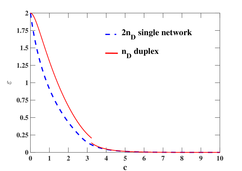
Refer to caption
Figure 6: Density of driver nodes ε=nD𝜀subscript𝑛𝐷\varepsilon=n_{D} for a duplex network composed by two Poisson networks with kA,in=kA,out=kB,in=kB,out=cdelimited-⟨⟩superscript𝑘𝐴𝑖𝑛delimited-⟨⟩superscript𝑘𝐴𝑜𝑢𝑡delimited-⟨⟩superscript𝑘𝐵𝑖𝑛delimited-⟨⟩superscript𝑘𝐵𝑜𝑢𝑡𝑐\left\langle{k^{A,in}}\right\rangle=\left\langle{k^{A,out}}\right\rangle=\left\langle{k^{B,in}}\right\rangle=\left\langle{k^{B,out}}\right\rangle=c is indicated with a solid red line and it clearly shows a phase transition for c=3.22233𝑐3.22233c=3.22233\ldots. In the dashed blue line we display the double of the number of driver nodes ε=2nD𝜀2subscript𝑛𝐷\varepsilon=2n_{D} for a single Poisson network with the same average degree c𝑐c, indicating the fraction of driver nodes necessary to control separately the two layers.

Here we consider the case of two Poisson networks with the same in/out average degree. In other words, we consider the situation in which kA,in=kA,out=kB,in=kB,out=cdelimited-⟨⟩superscript𝑘𝐴𝑖𝑛delimited-⟨⟩superscript𝑘𝐴𝑜𝑢𝑡delimited-⟨⟩superscript𝑘𝐵𝑖𝑛delimited-⟨⟩superscript𝑘𝐵𝑜𝑢𝑡𝑐\left\langle{k^{A,in}}\right\rangle=\left\langle{k^{A,out}}\right\rangle=\left\langle{k^{B,in}}\right\rangle=\left\langle{k^{B,out}}\right\rangle=c. The fraction nDsubscript𝑛𝐷n_{D} of nodes that are driver nodes of this duplex, is always larger than the double of the fraction of driver nodes in each of the layers taken in isolation (see Fig. 6). Moreover we observe that there is a phase transition in the controllability of these duplex networks, indicated by a discontinuity of nDsubscript𝑛𝐷n_{D} for c=c=3.22233𝑐superscript𝑐3.22233c=c^{\star}=3.22233\ldots (see Fig. 6). In order to derive these results, we assumed wiA=wiBsuperscriptsubscript𝑤𝑖𝐴superscriptsubscript𝑤𝑖𝐵w_{i}^{A}=w_{i}^{B} for i=1,2,3𝑖123i=1,2,3 and w^iA=w^iBsuperscriptsubscript^𝑤𝑖𝐴superscriptsubscript^𝑤𝑖𝐵\hat{w}_{i}^{A}=\hat{w}_{i}^{B} for i=1,2,3𝑖123i=1,2,3. Therefore the zero-temperature BP equations at the ensemble level (43)43(\ref{equncorr}) read,

w1subscript𝑤1\displaystyle w_{1} =\displaystyle= ec(1w^2),superscript𝑒𝑐1subscript^𝑤2\displaystyle e^{-c(1-\hat{w}_{2})},
w2subscript𝑤2\displaystyle w_{2} =\displaystyle= [1ecw^1],delimited-[]1superscript𝑒𝑐subscript^𝑤1\displaystyle\left[1-e^{-c\hat{w}_{1}}\right],
w3subscript𝑤3\displaystyle w_{3} =\displaystyle= 1w1w2,1subscript𝑤1subscript𝑤2\displaystyle 1-w_{1}-w_{2},
w^3subscript^𝑤3\displaystyle\hat{w}_{3} =\displaystyle= 1w^1w^2,1subscript^𝑤1subscript^𝑤2\displaystyle 1-\hat{w}_{1}-\hat{w}_{2},
w^1subscript^𝑤1\displaystyle\hat{w}_{1} =\displaystyle= ec(1w2)[1ecw1],superscript𝑒𝑐1subscript𝑤2delimited-[]1superscript𝑒𝑐subscript𝑤1\displaystyle e^{-c(1-w_{2})}\left[1-e^{-c{w}_{1}}\right],
w^2subscript^𝑤2\displaystyle\hat{w}_{2} =\displaystyle= [1ecw1+ecw1ec(1w2)].delimited-[]1superscript𝑒𝑐subscript𝑤1superscript𝑒𝑐subscript𝑤1superscript𝑒𝑐1subscript𝑤2\displaystyle\left[1-e^{-cw_{1}}+e^{-cw_{1}}e^{-c(1-w_{2})}\right].

The energy E𝐸E is given in this case by

E𝐸\displaystyle E =\displaystyle= 2[ec(1w^2)1+ecw^1]2[1ecw1][1ec(1w2)]+2c[w^1(1w2)+w1(1w^2)].2delimited-[]superscript𝑒𝑐1subscript^𝑤21superscript𝑒𝑐subscript^𝑤12delimited-[]1superscript𝑒𝑐subscript𝑤1delimited-[]1superscript𝑒𝑐1subscript𝑤22𝑐delimited-[]subscript^𝑤11subscript𝑤2subscript𝑤11subscript^𝑤2\displaystyle 2\left[e^{-c(1-\hat{w}_{2})}-1+e^{-c\hat{w}_{1}}\right]-2[1-e^{-cw_{1}}][1-e^{-c(1-w_{2})}]+2c\left[\hat{w}_{1}(1-w_{2})+w_{1}(1-\hat{w}_{2})\right]. (85)
Refer to caption
Figure 7: Plots of the functions w^1=h1(w^1,w^2)subscript^𝑤1subscript1subscript^𝑤1subscript^𝑤2\hat{w}_{1}=h_{1}(\hat{w}_{1},\hat{w}_{2}) and w^2=h2(w^1,w^2)subscript^𝑤2subscript2subscript^𝑤1subscript^𝑤2\hat{w}_{2}=h_{2}(\hat{w}_{1},\hat{w}_{2}) given by Eqs. (86a)(86b)86a86b(\ref{2w1hatsameDNsupp})-(\ref{2w2hatsameDNsupp}). The solution of the system of these two equations, corresponds to a crossing of the two curves. We show the emergence of two new solutions of this system of equations for c>c=3.22233𝑐superscript𝑐3.22233c>c^{\star}=3.22233\ldots. The critical point csuperscript𝑐c^{\star} characterize an hybrid phase transition in the controllability of the duplex network.
Refer to caption
Figure 8: Values of the probabilities {wi}i=1,2,3subscriptsubscript𝑤𝑖𝑖123\{w_{i}\}_{i=1,2,3} and w^i=1,2,3subscript^𝑤𝑖123\hat{w}_{i=1,2,3} plotted as a function of the average degree c𝑐c, for a duplex network formed by two Poisson layers with kA,in=kA,out=kB,in=kB,out=cdelimited-⟨⟩superscript𝑘𝐴𝑖𝑛delimited-⟨⟩superscript𝑘𝐴𝑜𝑢𝑡delimited-⟨⟩superscript𝑘𝐵𝑖𝑛delimited-⟨⟩superscript𝑘𝐵𝑜𝑢𝑡𝑐\left\langle{k^{A,in}}\right\rangle=\left\langle{k^{A,out}}\right\rangle=\left\langle{k^{B,in}}\right\rangle=\left\langle{k^{B,out}}\right\rangle=c. These probabilities are calculated directly from BP results obtained over 5 single realizations these multiplex networks with average degree c𝑐c and N=104𝑁superscript104N=10^{4}.

We notice that the equations for w^1subscript^𝑤1\hat{w}_{1} and w^2subscript^𝑤2\hat{w}_{2} can be rewritten to form a closed subsystem of equations,

w^1subscript^𝑤1\displaystyle\hat{w}_{1} =\displaystyle= h1(w^1,w^2)=ececw^1[1ecec(1w^2)]subscript1subscript^𝑤1subscript^𝑤2superscript𝑒𝑐superscript𝑒𝑐subscript^𝑤1delimited-[]1superscript𝑒𝑐superscript𝑒𝑐1subscript^𝑤2\displaystyle h_{1}(\hat{w}_{1},\hat{w}_{2})=e^{-ce^{-c\hat{w}_{1}}}\left[1-e^{-ce^{-c(1-\hat{w}_{2})}}\right] (86a)
w^2subscript^𝑤2\displaystyle\hat{w}_{2} =\displaystyle= h2(w^1,w^2)=[1ecec(1w^2)+ecec(1w^2)ececw^1]subscript2subscript^𝑤1subscript^𝑤2delimited-[]1superscript𝑒𝑐superscript𝑒𝑐1subscript^𝑤2superscript𝑒𝑐superscript𝑒𝑐1subscript^𝑤2superscript𝑒𝑐superscript𝑒𝑐subscript^𝑤1\displaystyle h_{2}(\hat{w}_{1},\hat{w}_{2})=\left[1-e^{-ce^{-c(1-\hat{w}_{2})}}+e^{-ce^{-c(1-\hat{w}_{2})}}e^{-ce^{-c\hat{w}_{1}}}\right] (86b)

from the solution of which the remaining quantities can be determined.

The value csuperscript𝑐c^{\star} of the average degree c𝑐c at which the discontinuity in the number of driver nodes nDsubscript𝑛𝐷n_{D} observed in Fig.6 occurs can be found by imposing that the two curves w^1=h1(w^1,w^2)subscript^𝑤1subscript1subscript^𝑤1subscript^𝑤2\hat{w}_{1}=h_{1}(\hat{w}_{1},\hat{w}_{2}) and w^2=h2(w^1,w^2)subscript^𝑤2subscript2subscript^𝑤1subscript^𝑤2\hat{w}_{2}=h_{2}(\hat{w}_{1},\hat{w}_{2}) of the plane w1,w2subscript𝑤1subscript𝑤2w_{1},w_{2} for c=c𝑐superscript𝑐c=c^{\star} are tangent to each other at their interception. These functions are plotted in Figure 7 where it is possible to observe that for c>c𝑐superscript𝑐c>c^{\star} the curves cross in three points while for c<c𝑐superscript𝑐c<c^{\star} they cross in one point, and at c=c𝑐superscript𝑐c=c^{\star} they are tangent to each other. The critical point csuperscript𝑐c^{\star} is found by imposing that the Eqs. (86) are satisfied together with the condition

|J|=0,𝐽0\displaystyle\left|J\right|=0, (87)

with J𝐽J indicating the Jacobian of the system of equations w^1=h1(w^1,w^2)subscript^𝑤1subscript1subscript^𝑤1subscript^𝑤2\hat{w}_{1}=h_{1}(\hat{w}_{1},\hat{w}_{2}) and w^2=h2(w^1,w^2)subscript^𝑤2subscript2subscript^𝑤1subscript^𝑤2\hat{w}_{2}=h_{2}(\hat{w}_{1},\hat{w}_{2}) given by

J=(1h1(w^1,w^2)w^1h1(w^1,w^2)w^2h2(w^1,w^2)w^11h2(w^1,w^2)w^2).𝐽1subscript1subscript^𝑤1subscript^𝑤2subscript^𝑤1subscript1subscript^𝑤1subscript^𝑤2subscript^𝑤2subscript2subscript^𝑤1subscript^𝑤2subscript^𝑤11subscript2subscript^𝑤1subscript^𝑤2subscript^𝑤2\displaystyle J=\left(\begin{array}[]{cc}1-\frac{\partial h_{1}(\hat{w}_{1},\hat{w}_{2})}{\partial\hat{w}_{1}}&-\frac{\partial h_{1}(\hat{w}_{1},\hat{w}_{2})}{\partial\hat{w}_{2}}\\ -\frac{\partial h_{2}(\hat{w}_{1},\hat{w}_{2})}{\partial\hat{w}_{1}}&1-\frac{\partial h_{2}(\hat{w}_{1},\hat{w}_{2})}{\partial\hat{w}_{2}}\end{array}\right). (89)

Imposing that Eqs. (86) and condition (87) are simultaneously satisfied, the solution c=3.222326106superscript𝑐3.222326106c^{\star}=3.222326106\ldots is found. For c<c𝑐superscript𝑐c<c^{\star} we observe that w3=w^3=0subscript𝑤3subscript^𝑤30w_{3}=\hat{w}_{3}=0. At csuperscript𝑐c^{\star} we observe a discontinuity in both w3subscript𝑤3w_{3} and w^3subscript^𝑤3\hat{w}_{3}, but for c>c𝑐superscript𝑐c>c^{\star} the functions h1(w^1,w^2)subscript1subscript^𝑤1subscript^𝑤2h_{1}(\hat{w}_{1},\hat{w}_{2}) and h2(w^1,w^2)subscript2subscript^𝑤1subscript^𝑤2h_{2}(\hat{w}_{1},\hat{w}_{2}) are analytic, and analyzing Eqs. (86a)(86b)86a86b(\ref{2w1hatsameDNsupp})-(\ref{2w2hatsameDNsupp}) we obtain the behavior of the order parameters w3subscript𝑤3w_{3} and w^3subscript^𝑤3\hat{w}_{3} for c>c𝑐superscript𝑐c>c^{\star}

w3w3subscript𝑤3superscriptsubscript𝑤3\displaystyle w_{3}-w_{3}^{\star} proportional-to\displaystyle\propto (cc)1/2superscript𝑐superscript𝑐12\displaystyle(c-c^{\star})^{1/2}
w^3w^3subscript^𝑤3superscriptsubscript^𝑤3\displaystyle\hat{w}_{3}-\hat{w}_{3}^{\star} proportional-to\displaystyle\propto (cc)1/2,superscript𝑐superscript𝑐12\displaystyle(c-c^{\star})^{1/2}, (90)

showing that the transition is hybrid.

We further characterize this phase transition evaluating the number of maximum matchings, i.e. the entropy value of the ground state solutions in the case of two poisson uncorrelated layers. The entropy density s𝑠s follows from Eq. (80) and it is plotted as a function of the average degree c𝑐c in Fig. 9. The entropy density presents a small jump at c=3.22233..superscript𝑐3.22233c^{*}=3.22233.. marking a change in the properties of the solutions.
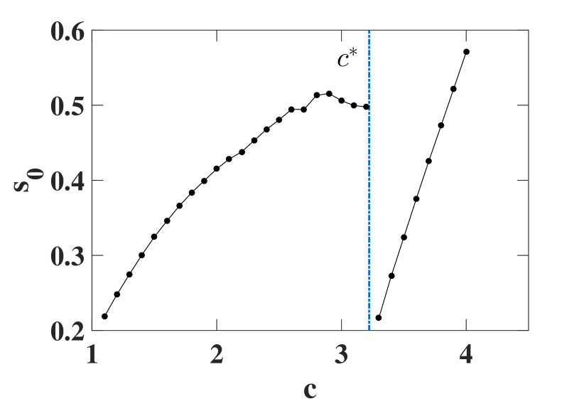
Refer to caption
Figure 9: Entropy density s𝑠s for a duplex network composed by two Poisson networks with kA,in=kA,out=kB,in=kB,out=cdelimited-⟨⟩superscript𝑘𝐴𝑖𝑛delimited-⟨⟩superscript𝑘𝐴𝑜𝑢𝑡delimited-⟨⟩superscript𝑘𝐵𝑖𝑛delimited-⟨⟩superscript𝑘𝐵𝑜𝑢𝑡𝑐\left\langle{k^{A,in}}\right\rangle=\left\langle{k^{A,out}}\right\rangle=\left\langle{k^{B,in}}\right\rangle=\left\langle{k^{B,out}}\right\rangle=c. At c=3.22233..superscript𝑐3.22233c^{*}=3.22233.., average degree corresponding to the hybrid phase transition, the entropy density s𝑠s displays a finite jump.

Here we want to modify the degree distribution of the duplex network characterized in this section, by changing the probability of nodes of low degree (degree 0,1,20120,1,2) that have been shown to be essential to determine the controllability of single layers PRL . Therefore we consider a duplex networks with degree distributions PAin(k)=PAout(k)=PBin(k)=PBout(k)=P(k)superscriptsubscript𝑃𝐴𝑖𝑛𝑘superscriptsubscript𝑃𝐴𝑜𝑢𝑡𝑘superscriptsubscript𝑃𝐵𝑖𝑛𝑘superscriptsubscript𝑃𝐵𝑜𝑢𝑡𝑘𝑃𝑘P_{A}^{in}(k)=P_{A}^{out}(k)=P_{B}^{in}(k)=P_{B}^{out}(k)=P(k) and with minimum degree is 2. In particular we consider P(k)𝑃𝑘P(k) given by

P(k)={0fork<2P(2)fork=2κ1k!ckfork[3,]𝑃𝑘cases0for𝑘2𝑃2for𝑘2𝜅1𝑘superscript𝑐𝑘for𝑘3\displaystyle P(k)=\left\{\begin{array}[]{lcc}0&\mbox{for}&{k<2}\\ P(2)&\mbox{for}&k=2\\ \kappa\frac{1}{k!}c^{k}&\mbox{for}&k\in[3,\infty]\end{array}\right. (94)

with κ𝜅\kappa indicating a normalization constant. In Fig. 10 (on the left) we show the phase diagram of this duplex network described by the dependence of the fraction of driver nodes nDsubscript𝑛𝐷n_{D} on c𝑐c and P(2)𝑃2P(2). The dark grey area defines the region where the zero-energy solution is stable, hence in which to control a duplex one needs only an infinitesimal fraction of driver nodes, i.e. nD=0subscript𝑛𝐷0n_{D}=0. These results are compared with the situation in which the two layers are controlled separately shown in Fig. 10 (on the right). The fraction of driver replica nodes of the duplex network is always larger that the double of the fraction of driver nodes in any single layer taken in isolation. Moreover the region in which the fully controllable solution is stable is the same for the duplex network, and for the single networks in the layers of the duplex network taken in isolation. This result is consistent with the theoretical expectations obtained in Sec. .4.2. In fact the in- and out-degree distributions of the two layers are the same.
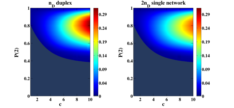
Refer to caption
Figure 10: On the left: the density of driver nodes nDsubscript𝑛𝐷n_{D} as a function of the parameters c𝑐c and P(2)𝑃2P(2) is plotted for duplex networks with PAin(k)=PAout(k)=PBin(k)=PBout(k)=P(k)superscriptsubscript𝑃𝐴𝑖𝑛𝑘superscriptsubscript𝑃𝐴𝑜𝑢𝑡𝑘superscriptsubscript𝑃𝐵𝑖𝑛𝑘superscriptsubscript𝑃𝐵𝑜𝑢𝑡𝑘𝑃𝑘P_{A}^{in}(k)=P_{A}^{out}(k)=P_{B}^{in}(k)=P_{B}^{out}(k)=P(k) and P(k)𝑃𝑘P(k) given by Eq. (94)94(\ref{pkinoutpoisson}). On the right: the double of the density of driver nodes nDsubscript𝑛𝐷n_{D} for single layers with degree distribution Pin(k)=Pout(k)=P(k)superscript𝑃𝑖𝑛𝑘superscript𝑃𝑜𝑢𝑡𝑘𝑃𝑘P^{in}(k)=P^{out}(k)=P(k) and P(k)𝑃𝑘P(k) given by (94)94(\ref{pkinoutpoisson}) is plotted as a function of c𝑐c and P(2)𝑃2P(2).

.4.5 Controllability of scale-free duplex networks

Following Sec. .4.4 we consider now the case of two uncorrelated layers composed by two power-law networks with P(kA,in)=P(kA,out)=P(kB,in)=P(kB,out)=P(k)kγ𝑃superscript𝑘𝐴𝑖𝑛𝑃superscript𝑘𝐴𝑜𝑢𝑡𝑃superscript𝑘𝐵𝑖𝑛𝑃superscript𝑘𝐵𝑜𝑢𝑡𝑃𝑘proportional-tosuperscript𝑘𝛾P(k^{A,in})=P(k^{A,out})=P(k^{B,in})=P(k^{B,out})=P(k)\propto k^{-\gamma} and minimal degree m=1𝑚1m=1. Similarly to the poisson case, the fraction nDsubscript𝑛𝐷n_{D} of driver nodes of this duplex, is always larger than the double of the fraction of driver nodes in each of the layers taken in isolation (see Fig. 11).
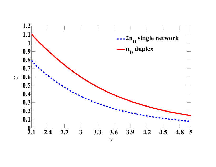
Refer to caption
Figure 11: Density of driver nodes ε=nD𝜀subscript𝑛𝐷\varepsilon=n_{D} for a duplex network composed by two power-law networks with P(kA,in)=P(kA,out)=P(kB,in)=P(kB,out)=P(k)kγ𝑃superscript𝑘𝐴𝑖𝑛𝑃superscript𝑘𝐴𝑜𝑢𝑡𝑃superscript𝑘𝐵𝑖𝑛𝑃superscript𝑘𝐵𝑜𝑢𝑡𝑃𝑘proportional-tosuperscript𝑘𝛾P(k^{A,in})=P(k^{A,out})=P(k^{B,in})=P(k^{B,out})=P(k)\propto k^{-\gamma} and minimal degree m=1𝑚1m=1 as a function of γ𝛾\gamma (indicated with a solid red line). The minimum in/out degree 111 and the maximum in/out degree is given by the structural cutoff with N=104𝑁superscript104N=10^{4}. In the dashed blue line we display the double of the number of driver nodes ε=2nD𝜀2subscript𝑛𝐷\varepsilon=2n_{D} for a single power-law network with the same in/out degree distributions P(k)𝑃𝑘P(k), indicating the fraction of driver nodes necessary to control separately the two layers.

Moreover, low-degree nodes significantly affect the controllability of duplex networks formed by scale-free networks. We consider a duplex network with PAin(k)=PAout(k)=PBin(k)=PBout(k)=P(k)superscriptsubscript𝑃𝐴𝑖𝑛𝑘superscriptsubscript𝑃𝐴𝑜𝑢𝑡𝑘superscriptsubscript𝑃𝐵𝑖𝑛𝑘superscriptsubscript𝑃𝐵𝑜𝑢𝑡𝑘𝑃𝑘P_{A}^{in}(k)=P_{A}^{out}(k)=P_{B}^{in}(k)=P_{B}^{out}(k)=P(k) and P(k)𝑃𝑘P(k) given by

P(k)={0ifk=1P(2)ifk=2κkγifk[3,M]𝑃𝑘cases0if𝑘1𝑃2if𝑘2𝜅superscript𝑘𝛾if𝑘3𝑀\displaystyle P(k)=\left\{\begin{array}[]{lcc}0&\mbox{if}&{k=1}\\ P(2)&\mbox{if}&k=2\\ \kappa k^{-\gamma}&\mbox{if}&k\in[3,M]\end{array}\right. (98)

with κ𝜅\kappa indicating the normalization sum and γ>2𝛾2\gamma>2. We consider uncorrelated networks, therefore the cutoff M𝑀M on the degrees of the nodes will be given by

M=min(N,{[1P(1)P(2)]N}1/(γ1)).𝑀𝑁superscriptdelimited-[]1𝑃1𝑃2𝑁1𝛾1\displaystyle M=\min(\sqrt{N},\left\{[1-P(1)-P(2)]N\right\}^{1/(\gamma-1)}). (99)

In other words, the cutoff M𝑀M is given by the minimum between the structural cutoff of the network and the natural cutoff of the degree distribution. In Fig. 12 (on the left) we present the phase diagram of a duplex network displaying the fraction of driver nodes nDsubscript𝑛𝐷n_{D} as a function of the parameters γ𝛾\gamma and P(2)𝑃2P(2). The dark grey area is associated with the stable zero-energy solution while outside this region, the minimum fraction of driver nodes necessary for a full duplex control follows the colorcode. We compare these results with the situation in which the two layers are controlled separately (on the right). We observe that the number of driver replica nodes in the duplex is always greater than the total number of driver nodes of the single layer taken in isolation, provided that the duplex network is not fully controllable. We note that for the degree distribution considered in this case, consistently with the theoretical results obtained in Sec. .4.2, we observe that the region for the stability of the full controllability solution for the duplex network is the same of the region for the stability of the full controllability solution in the single layers. Finally , in Fig. 13 we compare our theoretical results for the ensemble of duplex networks with degree distributions PAin(k)=PAout(k)=PBin(k)=PBout(k)=P(k)superscriptsubscript𝑃𝐴𝑖𝑛𝑘superscriptsubscript𝑃𝐴𝑜𝑢𝑡𝑘superscriptsubscript𝑃𝐵𝑖𝑛𝑘superscriptsubscript𝑃𝐵𝑜𝑢𝑡𝑘𝑃𝑘P_{A}^{in}(k)=P_{A}^{out}(k)=P_{B}^{in}(k)=P_{B}^{out}(k)=P(k) and P(k)𝑃𝑘P(k) given by Eq. (98)98(\ref{pkinout}), with those obtained by the message-passing (BP) algorithm, finding a good agreement (Eq. 70 returns a limit value for P(2)𝑃2P(2) equal to 0.1819470.1819470.181947).

Refer to caption
Figure 12: On the left: the density of driver nodes nDsubscript𝑛𝐷n_{D} as a function of the parameters γ𝛾\gamma and P(2)𝑃2P(2) for duplex networks of N=106𝑁superscript106N=10^{6} nodes with degree distributions PAin(k)=PAout(k)=PBin(k)=PBout(k)=P(k)superscriptsubscript𝑃𝐴𝑖𝑛𝑘superscriptsubscript𝑃𝐴𝑜𝑢𝑡𝑘superscriptsubscript𝑃𝐵𝑖𝑛𝑘superscriptsubscript𝑃𝐵𝑜𝑢𝑡𝑘𝑃𝑘P_{A}^{in}(k)=P_{A}^{out}(k)=P_{B}^{in}(k)=P_{B}^{out}(k)=P(k) and P(k)𝑃𝑘P(k) given by Eq. (98)98(\ref{pkinout}). On the right: double of the density of driver nodes nDsubscript𝑛𝐷n_{D} as a function of the parameters γ𝛾\gamma and P(2)𝑃2P(2) for single networks of N=106𝑁superscript106N=10^{6} nodes with degree distributions Pin(k)=Pout(k)=P(k)superscript𝑃𝑖𝑛𝑘superscript𝑃𝑜𝑢𝑡𝑘𝑃𝑘P^{in}(k)=P^{out}(k)=P(k) and P(k)𝑃𝑘P(k) given by Eq. (98)98(\ref{pkinout}).
Refer to caption
Figure 13: Density of driver nodes nDsubscript𝑛𝐷n_{D} as a function of P(2)𝑃2P(2) for a duplex network with PAin(k)=PAout(k)=PBin(k)=PBout(k)=P(k)superscriptsubscript𝑃𝐴𝑖𝑛𝑘superscriptsubscript𝑃𝐴𝑜𝑢𝑡𝑘superscriptsubscript𝑃𝐵𝑖𝑛𝑘superscriptsubscript𝑃𝐵𝑜𝑢𝑡𝑘𝑃𝑘P_{A}^{in}(k)=P_{A}^{out}(k)=P_{B}^{in}(k)=P_{B}^{out}(k)=P(k), P(k)𝑃𝑘P(k) given by Eq. (98)98(\ref{pkinout}) and γ=2.3𝛾2.3\gamma=2.3. The fraction of driver nodes computed with the zero-temperature BP (Max-Sum) algorithm on a duplex network of N=104𝑁superscript104N=10^{4} nodes (averaged over 252525 network realizations) is compared with the theoretical expectation for the density nDsubscript𝑛𝐷n_{D} in an ensemble of random duplex networks with the given degree distributions.

.5 Effect of degree correlations on controllability of multiplex networks

In order to analyze the effect of degree correlations PhysReports on the controllability of multiplex networks, we correlate the degree of the replica nodes in the two layers of a duplex network formed by layer A𝐴A and layer B𝐵B. In particular we consider two cases: a duplex network in which only the low in-degree nodes (nodes of in-degree 0,1,20120,1,2 ) are correlated and a duplex networks in which the in-degrees of the replica nodes are correlated independently on their value. For each case, we define the joint in-degree distribution Pin(kA,kB)superscript𝑃𝑖𝑛superscript𝑘𝐴superscript𝑘𝐵P^{in}(k^{A},k^{B}) between layers and the corresponding expression of the zero-temperature BP equations in the correlated ensemble of networks.

In the first case we consider a joint in-degree distribution Pin(kA,kB)superscript𝑃𝑖𝑛superscript𝑘𝐴superscript𝑘𝐵P^{in}(k^{A},k^{B}) given by

Pin(kA,kB)={pδkB,kAP(kA)+(1p)P(kA)P(kB),forkA2(1p)P(kA)P(kB),for kA>2kB2pP(kB)CP(kA)+(1p)P(kA)P(kB),for kA>2kB>2,subscript𝑃𝑖𝑛superscript𝑘𝐴superscript𝑘𝐵cases𝑝subscript𝛿superscript𝑘𝐵superscript𝑘𝐴𝑃superscript𝑘𝐴1𝑝𝑃superscript𝑘𝐴𝑃superscript𝑘𝐵forsuperscript𝑘𝐴21𝑝𝑃superscript𝑘𝐴𝑃superscript𝑘𝐵for formulae-sequencesuperscript𝑘𝐴2superscript𝑘𝐵2𝑝𝑃superscript𝑘𝐵𝐶𝑃superscript𝑘𝐴1𝑝𝑃superscript𝑘𝐴𝑃superscript𝑘𝐵for formulae-sequencesuperscript𝑘𝐴2superscript𝑘𝐵2\displaystyle P_{in}(k^{A},k^{B})=\left\{\begin{array}[]{lll}p\delta_{k^{B},k^{A}}P(k^{A})+(1-p)P(k^{A})P(k^{B}),&\mbox{for}&k^{A}\leq 2\\ (1-p)P(k^{A})P(k^{B}),&\mbox{for }&k^{A}>2\quad k^{B}\leq 2\\ p\frac{P(k^{B})}{C}P(k^{A})+(1-p)P(k^{A})P(k^{B}),&\mbox{for }&k^{A}>2\quad k^{B}>2\end{array}\right., (101)

where C=1k2P(k)𝐶1subscript𝑘2𝑃𝑘C=1-\sum_{k\leq 2}P(k) where P(k)𝑃𝑘P(k) is a given normalized degree distribution. The distributions of the fields over the links of this ensemble of networks are given by

𝒫α(hα)subscript𝒫𝛼superscript𝛼\displaystyle{\cal P}_{\alpha}(h^{\alpha}) =\displaystyle= w1αδ(hα1)+w2αδ(hα+1)+w3αδ(hα),superscriptsubscript𝑤1𝛼𝛿superscript𝛼1superscriptsubscript𝑤2𝛼𝛿superscript𝛼1superscriptsubscript𝑤3𝛼𝛿superscript𝛼\displaystyle w_{1}^{\alpha}\delta(h^{\alpha}-1)+w_{2}^{\alpha}\delta(h^{\alpha}+1)+w_{3}^{\alpha}\delta(h^{\alpha}),
𝒫^α(h^α)subscript^𝒫𝛼superscript^𝛼\displaystyle\hat{{\cal P}}_{\alpha}(\hat{h}^{\alpha}) =\displaystyle= w^1αδ(h^α1)+w^2αδ(h^α+1)+w^3αδ(h^α),superscriptsubscript^𝑤1𝛼𝛿superscript^𝛼1superscriptsubscript^𝑤2𝛼𝛿superscript^𝛼1superscriptsubscript^𝑤3𝛼𝛿superscript^𝛼\displaystyle\hat{w}_{1}^{\alpha}\delta(\hat{h}^{\alpha}-1)+\hat{w}_{2}^{\alpha}\delta(\hat{h}^{\alpha}+1)+\hat{w}_{3}^{\alpha}\delta(\hat{h}^{\alpha}), (102)

where α=A,B𝛼𝐴𝐵\alpha=A,B and where the probabilities w1α,w2α,w3αsuperscriptsubscript𝑤1𝛼superscriptsubscript𝑤2𝛼superscriptsubscript𝑤3𝛼w_{1}^{\alpha},w_{2}^{\alpha},w_{3}^{\alpha} are normalized w1α+w2α+w3α=1superscriptsubscript𝑤1𝛼superscriptsubscript𝑤2𝛼superscriptsubscript𝑤3𝛼1w_{1}^{\alpha}+w_{2}^{\alpha}+w_{3}^{\alpha}=1 as well as the probabilities w^1α,w^2α,w^3αsuperscriptsubscript^𝑤1𝛼superscriptsubscript^𝑤2𝛼superscriptsubscript^𝑤3𝛼\hat{w}_{1}^{\alpha},\hat{w}_{2}^{\alpha},\hat{w}_{3}^{\alpha} that satisfy the equation w^1α+w^2α+w^3α=1superscriptsubscript^𝑤1𝛼superscriptsubscript^𝑤2𝛼superscriptsubscript^𝑤3𝛼1\hat{w}_{1}^{\alpha}+\hat{w}_{2}^{\alpha}+\hat{w}_{3}^{\alpha}=1. The zero-temperature BP (Max-Sum) equations (39) averaged over this ensemble of networks can be expressed in terms of the probabilities {wiα}i=1,2,3subscriptsuperscriptsubscript𝑤𝑖𝛼𝑖123\{w_{i}^{\alpha}\}_{i=1,2,3} and {wiα}i=1,2,3subscriptsuperscriptsubscript𝑤𝑖𝛼𝑖123\{w_{i}^{\alpha}\}_{i=1,2,3} as

w^1subscript^𝑤1\displaystyle\hat{w}_{1} =\displaystyle= p[P(1)kw1+2P(2)kw2(1(1w1)2)+(G1(w2)P(1)k2P(2)kw2)(1G~0(1w1))]𝑝delimited-[]𝑃1delimited-⟨⟩𝑘subscript𝑤12𝑃2delimited-⟨⟩𝑘subscript𝑤21superscript1subscript𝑤12subscript𝐺1subscript𝑤2𝑃1delimited-⟨⟩𝑘2𝑃2delimited-⟨⟩𝑘subscript𝑤21subscript~𝐺01subscript𝑤1\displaystyle p\left[\frac{P(1)}{\langle{k}\rangle}w_{1}+\frac{2P(2)}{\langle{k}\rangle}w_{2}(1-(1-w_{1})^{2})+(G_{1}(w_{2})-\frac{P(1)}{\langle{k}\rangle}-\frac{2P(2)}{\langle{k}\rangle}w_{2})(1-\tilde{G}_{0}(1-w_{1}))\right] (103a)
+(1p)G1(w2)[1G0(1w1)]1𝑝subscript𝐺1subscript𝑤2delimited-[]1subscript𝐺01subscript𝑤1\displaystyle+(1-p)G_{1}(w_{2})\left[1-G_{0}(1-{w}_{1})\right]
w^2subscript^𝑤2\displaystyle\hat{w}_{2} =\displaystyle= p[P(1)kw2+2P(2)k(w1+w22(1w1))+1P(1)k2P(2)k\displaystyle p\left[\frac{P(1)}{\langle{k}\rangle}w_{2}+\frac{2P(2)}{\langle{k}\rangle}(w_{1}+w_{2}^{2}(1-w1))+1-\frac{P(1)}{\langle{k}\rangle}-\frac{2P(2)}{\langle{k}\rangle}\right. (103b)
(G1(1w1)P(1)k2P(2)k(1w1))(1G~0(w2))]\displaystyle\left.-(G_{1}(1-w_{1})-\frac{P(1)}{\langle{k}\rangle}-\frac{2P(2)}{\langle{k}\rangle}(1-w_{1}))(1-\tilde{G}_{0}(w_{2}))\right]
+(1p)[1G1(1w1)+G1(1w1)G0(w2)]1𝑝delimited-[]1subscript𝐺11subscript𝑤1subscript𝐺11subscript𝑤1subscript𝐺0subscript𝑤2\displaystyle+(1-p)\left[1-G_{1}(1-w_{1})+G_{1}(1-w_{1})G_{0}\left(w_{2}\right)\right]

where

G0(z)subscript𝐺0𝑧\displaystyle{G}_{0}(z) =\displaystyle= kP(k)zksubscript𝑘𝑃𝑘superscript𝑧𝑘\displaystyle\sum_{k}{P(k)}z^{k}
G1(z)subscript𝐺1𝑧\displaystyle{G}_{1}(z) =\displaystyle= kkkP(k)zksubscript𝑘𝑘delimited-⟨⟩𝑘𝑃𝑘superscript𝑧𝑘\displaystyle\sum_{k}\frac{k}{\langle{k}\rangle}P(k)z^{k}
G~0(z)subscript~𝐺0𝑧\displaystyle\tilde{G}_{0}(z) =\displaystyle= k3P(k)Czk.subscript𝑘3𝑃𝑘𝐶superscript𝑧𝑘\displaystyle\sum_{k\geq 3}\frac{P(k)}{C}z^{k}. (104)

Finally the energy E𝐸E is given by

E𝐸\displaystyle E =\displaystyle= 2{G0(w^2)[1G0(1w^1)]}+2k[w^1(1w2)+w1(1w^2)]2(1p){[1G0(1w1)][1G0(w2)]}2subscript𝐺0subscript^𝑤2delimited-[]1subscript𝐺01subscript^𝑤12delimited-⟨⟩𝑘delimited-[]subscript^𝑤11subscript𝑤2subscript𝑤11subscript^𝑤221𝑝delimited-[]1subscript𝐺01subscript𝑤1delimited-[]1subscript𝐺0subscript𝑤2\displaystyle 2\left\{G_{0}\left(\hat{w}_{2}\right)-\left[1-G_{0}(1-\hat{w}_{1})\right]\right\}+2{\langle{k}\rangle}\left[\hat{w}_{1}(1-w_{2})+w_{1}(1-\hat{w}_{2})\right]-2(1-p)\left\{[1-G_{0}(1-w_{1})][1-G_{0}(w_{2})]\right\} (105)
\displaystyle- 2p{P(1)w1(1w2)+P(2)(1(1w1)2)(1w22)+C(1G~0(1w1))(1G~0(w2))}2𝑝𝑃1subscript𝑤11subscript𝑤2𝑃21superscript1subscript𝑤121superscriptsubscript𝑤22𝐶1subscript~𝐺01subscript𝑤11subscript~𝐺0subscript𝑤2\displaystyle 2p\left\{P(1)w_{1}(1-w_{2})+P(2)(1-(1-w_{1})^{2})(1-w_{2}^{2})+C(1-\tilde{G}_{0}(1-w_{1}))(1-\tilde{G}_{0}(w_{2}))\right\}

In the second case we consider the joint degree distribution Pin(kA,kB)superscript𝑃𝑖𝑛superscript𝑘𝐴superscript𝑘𝐵P^{in}(k^{A},k^{B}) given by

Pin(kA,kB)=pδkB,kAP(kA)+(1p)P(kA)P(kB),superscript𝑃𝑖𝑛superscript𝑘𝐴superscript𝑘𝐵𝑝subscript𝛿superscript𝑘𝐵superscript𝑘𝐴𝑃superscript𝑘𝐴1𝑝𝑃superscript𝑘𝐴𝑃superscript𝑘𝐵\displaystyle P^{in}(k^{A},k^{B})=p\delta_{k^{B},k^{A}}P(k^{A})+(1-p)P(k^{A})P(k^{B}), (106)

where P(k)𝑃𝑘P(k) is a given normalized degree distribution. The distributions of the fields over the links of this ensemble of duplex networks are given by

𝒫α(hα)subscript𝒫𝛼superscript𝛼\displaystyle{\cal P}_{\alpha}(h^{\alpha}) =\displaystyle= w1αδ(hα1)+w2αδ(hα+1)+w3αδ(hα),superscriptsubscript𝑤1𝛼𝛿superscript𝛼1superscriptsubscript𝑤2𝛼𝛿superscript𝛼1superscriptsubscript𝑤3𝛼𝛿superscript𝛼\displaystyle w_{1}^{\alpha}\delta(h^{\alpha}-1)+w_{2}^{\alpha}\delta(h^{\alpha}+1)+w_{3}^{\alpha}\delta(h^{\alpha}),
𝒫^α(h^α)subscript^𝒫𝛼superscript^𝛼\displaystyle\hat{{\cal P}}_{\alpha}(\hat{h}^{\alpha}) =\displaystyle= w^1αδ(h^α1)+w^2αδ(h^α+1)+w^3αδ(h^α),superscriptsubscript^𝑤1𝛼𝛿superscript^𝛼1superscriptsubscript^𝑤2𝛼𝛿superscript^𝛼1superscriptsubscript^𝑤3𝛼𝛿superscript^𝛼\displaystyle\hat{w}_{1}^{\alpha}\delta(\hat{h}^{\alpha}-1)+\hat{w}_{2}^{\alpha}\delta(\hat{h}^{\alpha}+1)+\hat{w}_{3}^{\alpha}\delta(\hat{h}^{\alpha}), (107)

where α=A,B𝛼𝐴𝐵\alpha=A,B and where the probabilities w1α,w2α,w3αsuperscriptsubscript𝑤1𝛼superscriptsubscript𝑤2𝛼superscriptsubscript𝑤3𝛼w_{1}^{\alpha},w_{2}^{\alpha},w_{3}^{\alpha} are normalized w1α+w2α+w3α=1superscriptsubscript𝑤1𝛼superscriptsubscript𝑤2𝛼superscriptsubscript𝑤3𝛼1w_{1}^{\alpha}+w_{2}^{\alpha}+w_{3}^{\alpha}=1 as well as the probabilities w^1α,w^2α,w^3αsuperscriptsubscript^𝑤1𝛼superscriptsubscript^𝑤2𝛼superscriptsubscript^𝑤3𝛼\hat{w}_{1}^{\alpha},\hat{w}_{2}^{\alpha},\hat{w}_{3}^{\alpha} that satisfy the equation w^1α+w^2α+w^3α=1superscriptsubscript^𝑤1𝛼superscriptsubscript^𝑤2𝛼superscriptsubscript^𝑤3𝛼1\hat{w}_{1}^{\alpha}+\hat{w}_{2}^{\alpha}+\hat{w}_{3}^{\alpha}=1. We get the equations

w^1subscript^𝑤1\displaystyle\hat{w}_{1} =\displaystyle= p[G1(w2)(1w1)G1(w2(1w1))]+(1p)G1(w2)[1G0(1w1)]𝑝delimited-[]subscript𝐺1subscript𝑤21subscript𝑤1subscript𝐺1subscript𝑤21subscript𝑤11𝑝subscript𝐺1subscript𝑤2delimited-[]1subscript𝐺01subscript𝑤1\displaystyle p\left[G_{1}(w_{2})-(1-w_{1})G_{1}(w_{2}(1-w_{1}))\right]+(1-p)G_{1}(w_{2})\left[1-G_{0}(1-{w}_{1})\right] (108a)
w^2subscript^𝑤2\displaystyle\hat{w}_{2} =\displaystyle= p[1G1(1w1)+w2G1(w2(1w1))]+(1p)[1G1(1w1)+G1(1w1)G0(w2)],𝑝delimited-[]1subscript𝐺11subscript𝑤1subscript𝑤2subscript𝐺1subscript𝑤21subscript𝑤11𝑝delimited-[]1subscript𝐺11subscript𝑤1subscript𝐺11subscript𝑤1subscript𝐺0subscript𝑤2\displaystyle p\left[1-G_{1}(1-w_{1})+w_{2}G_{1}(w_{2}(1-w_{1}))\right]+(1-p)\left[1-G_{1}(1-w_{1})+G_{1}(1-w_{1})G_{0}\left(w_{2}\right)\right], (108b)

where the generating functions G0(z)subscript𝐺0𝑧G_{0}(z) and G1(z)subscript𝐺1𝑧G_{1}(z) are defined as

G0(z)=kP(k)zk,subscript𝐺0𝑧subscript𝑘𝑃𝑘superscript𝑧𝑘\displaystyle{G}_{0}(z)=\sum_{k}{P(k)}z^{k},
G1(z)=kkkP(k)zk.subscript𝐺1𝑧subscript𝑘𝑘delimited-⟨⟩𝑘𝑃𝑘superscript𝑧𝑘\displaystyle{G}_{1}(z)=\sum_{k}\frac{k}{\langle{k}\rangle}P(k)z^{k}. (109)

The energy E𝐸E in this ensemble is given by

E𝐸\displaystyle E =\displaystyle= 2{G0(w^2)[1G0(1w^1)]}+2k[w^1(1w2)+w1(1w^2)]2subscript𝐺0subscript^𝑤2delimited-[]1subscript𝐺01subscript^𝑤12delimited-⟨⟩𝑘delimited-[]subscript^𝑤11subscript𝑤2subscript𝑤11subscript^𝑤2\displaystyle 2\left\{G_{0}\left(\hat{w}_{2}\right)-\left[1-G_{0}(1-\hat{w}_{1})\right]\right\}+2{\langle{k}\rangle}\left[\hat{w}_{1}(1-w_{2})+w_{1}(1-\hat{w}_{2})\right] (110)
\displaystyle- 2(1p){[1G0(1w1)][1G0(w2)]}2p{1G0(1w1)G0(w2)+G0(w2(1w1))}21𝑝delimited-[]1subscript𝐺01subscript𝑤1delimited-[]1subscript𝐺0subscript𝑤22𝑝1subscript𝐺01subscript𝑤1subscript𝐺0subscript𝑤2subscript𝐺0subscript𝑤21subscript𝑤1\displaystyle 2(1-p)\left\{[1-G_{0}(1-w_{1})][1-G_{0}(w_{2})]\right\}-2p\left\{1-G_{0}(1-w_{1})-G_{0}(w_{2})+G_{0}(w_{2}(1-w_{1}))\right\}

The degree correlation of low in-degree nodes can modify the number of driver nodes nDsubscript𝑛𝐷n_{D} found in duplex networks (see Fig. 14 for the case of a duplex network formed by Poisson layers with kA,in=kA,out=kB,in=kB,out=cdelimited-⟨⟩superscript𝑘𝐴𝑖𝑛delimited-⟨⟩superscript𝑘𝐴𝑜𝑢𝑡delimited-⟨⟩superscript𝑘𝐵𝑖𝑛delimited-⟨⟩superscript𝑘𝐵𝑜𝑢𝑡𝑐\left\langle{k^{A,in}}\right\rangle=\left\langle{k^{A,out}}\right\rangle=\left\langle{k^{B,in}}\right\rangle=\left\langle{k^{B,out}}\right\rangle=c). Once the low in-degree nodes are correlated, correlating also the other in-degrees of the network does not change substantially the number of driver nodes nDsubscript𝑛𝐷n_{D} as discussed in the main body of the paper.
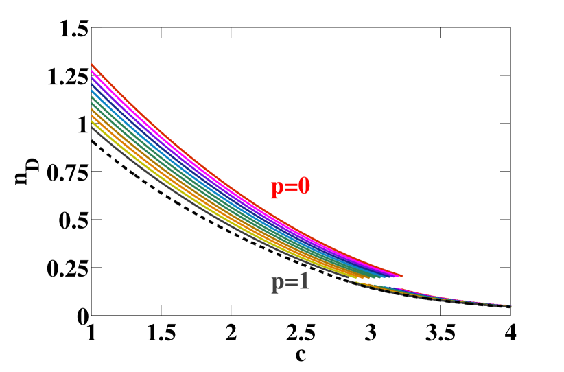
Refer to caption
Figure 14: The density of the driver nodes nDsubscript𝑛𝐷n_{D} in a duplex network formed by two Poisson networks with kA,in=kA,out=kB,in=kB,out=cdelimited-⟨⟩superscript𝑘𝐴𝑖𝑛delimited-⟨⟩superscript𝑘𝐴𝑜𝑢𝑡delimited-⟨⟩superscript𝑘𝐵𝑖𝑛delimited-⟨⟩superscript𝑘𝐵𝑜𝑢𝑡𝑐\left\langle{k^{A,in}}\right\rangle=\left\langle{k^{A,out}}\right\rangle=\left\langle{k^{B,in}}\right\rangle=\left\langle{k^{B,out}}\right\rangle=c and with correlated low in-degrees is plotted as function of c𝑐c for different values of p𝑝p. The result for the two separate layers is shown in black (dashed curve) while the situation for uncorrelated layers is shown in red. The value of p𝑝p increases going from the red curve (p=0𝑝0p=0) to the grey curve (p=1𝑝1p=1).

References

  • (1) Boccaletti, S. et al. The structure and dynamics of multilayer networks. Phys. Rep. 544, 1–122 (2014).
  • (2) Kivela, M. et al. Multilayer networks. J. Compl. Net. 2, 203–271 (2014).
  • (3) Delpini, D. et al. Evolution of controllability in interbank networks. Sci. Rep. 3, 1626 (2013).
  • (4) Battiston, S., Puliga, M., Kaushik, R., Tasca, P. & Caldarelli, G. DebtRank: too central to fail? Financial networks, the FED and systemic risk. Sci. Rep. 2, 541 (2012).
  • (5) Csermely, P., Korcsmáros, T., Kiss, H. J. M., London, G. & Nussinov, R. Structure and dynamics of molecular networks: A novel paradigm of drug discovery: A comprehensive review. Pharmacol. Ther. 138, 333–408 (2013). eprint 1210.0330.
  • (6) Bullmore, E. & Sporns, O. Complex brain networks: graph theoretical analysis of structural and functional systems. Nat. Rev. Neurosci. 10, 186–198 (2009).
  • (7) Bonifazi, P. et al. GABAergic hub neurons orchestrate synchrony in developing hippocampal networks. Science 326, 1419–24 (2009).
  • (8) Power, J. D. et al. Functional network organization of the human brain. Neuron 72, 665–78 (2011).
  • (9) Reis, S. D. S. et al. Avoiding catastrophic failure in correlated networks of networks. Nat. Phys. 10, 762–767 (2014).
  • (10) Castellani, G., Intrator, N. & Remondini, D. Systems biology and brain activity in neuronal pathways by smart device and advanced signal processing. Front. Genet. 5, 253 (2014).
  • (11) Lin, C. T. Structural controllability. IEEE T. Automat. Contr. 19, 201–208 (1974).
  • (12) Liu, Y.-Y., Slotine, J.-J. & Barabási, A.-L. Controllability of complex networks. Nature 473, 167–173 (2011).
  • (13) Pósfai, M., Liu, Y.-Y., Slotine, J.-J. & Barabási, A.-L. Effect of correlations on network controllability. Sci. Rep. 3, 1067 (2013).
  • (14) Ruths, J. & Ruths, D. Control profiles of complex networks. Science 343, 1373–6 (2014).
  • (15) Campbell, C., Shea, K. & Albert, R. Comment on ”Control profiles of complex networks”. Science 346, 561 (2014).
  • (16) Menichetti, G., Dall’Asta, L. & Bianconi, G. Network Controllability Is Determined by the Density of Low In-Degree and Out-Degree Nodes. Phys. Rev. Lett. 113, 078701 (2014).
  • (17) Nepusz, T. & Vicsek, T. Controlling edge dynamics in complex networks. Nat. Phys. 8, 568–573 (2012). eprint 1112.5945.
  • (18) Yan, G. et al. Spectrum of controlling and observing complex networks. Nat. Phys. 11, 779–786 (2015).
  • (19) Liu, Y. Y.-y., Slotine, J.-j. J. & Barabasi, A. Control Centrality and Hierarchical Structure in Complex Networks. B. Am. Phys. Soc. 7, 1–14 (2012). eprint arXiv:1203.2655v1.
  • (20) Slotine, J.-J. E. & Li, W. Applied Nonlinear Control (Prentice-Hall, 1991).
  • (21) Wang, X. F. & Chen, G. Pinning control of scale-free dynamical networks. Physica A 310, 521–531 (2002).
  • (22) Sorrentino, F., di Bernardo, M., Garofalo, F. & Chen, G. Controllability of complex networks via pinning. Phys. Rev. E 75, 046103 (2007).
  • (23) Gutiérrez, R., Sendiña Nadal, I., Zanin, M., Papo, D. & Boccaletti, S. Targeting the dynamics of complex networks. Sci. Rep. 2, 396 (2012).
  • (24) Porfiri, M. & di Bernardo, M. Criteria for global pinning-controllability of complex networks. Automatica 44, 3100–3106 (2008).
  • (25) De Lellis, P., di Bernardo, M. & Garofalo, F. Synchronization of complex networks through local adaptive coupling. Chaos 18, 037110 (2008).
  • (26) Wang, W.-X., Ni, X., Lai, Y.-C. & Grebogi, C. Optimizing controllability of complex networks by minimum structural perturbations. Phys. Rev. E 85, 026115 (2012).
  • (27) Yan, G., Ren, J., Lai, Y.-C., Lai, C.-H. & Li, B. Controlling Complex Networks: How Much Energy Is Needed? Phys. Rev. Lett. 108, 218703 (2012).
  • (28) Cornelius, S. P., Kath, W. L. & Motter, A. E. Realistic control of network dynamics. Nat. Comm. 4, 1942 (2013).
  • (29) Sun, J. & Motter, A. E. Controllability Transition and Nonlocality in Network Control. Phys. Rev. Lett. 110, 208701 (2013).
  • (30) Yuan, Z., Zhao, C., Di, Z., Wang, W.-X. & Lai, Y.-C. Exact controllability of complex networks. Nat. Comm. 4, 2447 (2013).
  • (31) Zdeborová, L. & Mézard, M. The number of matchings in random graphs. J. Stat. Mech. 2006, P05003–P05003 (2006).
  • (32) Altarelli, F., Braunstein, A., Ramezanpour, A. & Zecchina, R. Stochastic Matching Problem. Phys. Rev. Lett. 106, 190601 (2011).
  • (33) Mézard, M. & Parisi, G. The Bethe lattice spin glass revisited. Eur. Phys. J. B 20, 217–233 (2001).
  • (34) Martin, O. C., Monasson, R. & Zecchina, R. Statistical mechanics methods and phase transitions in optimization problems. Theor. Comput. Sci. 265, 3–67 (2001).
  • (35) Hartmann, A. K. & Weigt, M. Phase Transitions in Combinatorial Optimization Problems: Basics, Algorithms and Statistical Mechanics, vol. 4 (John Wiley and Sons, 2005).
  • (36) Mézard, M. & Montanari, A. Information, Physics, and Computation (Oxford University Press,2009).
  • (37) Liu, Y.-Y., Slotine, J.-J. & Barabási, A.-L. Observability of complex systems. P. Natl. Acad. Sci. USA 110, 2460–5 (2013).
  • (38) Gao, J., Liu, Y.-Y., D’Souza, R. M. & Barabási, A.-L. Target control of complex networks. Nat. Comm. 5, 5415 (2014).
  • (39) Buldyrev, S. V., Parshani, R., Paul, G., Stanley, H. E. & Havlin, S. Catastrophic cascade of failures in interdependent networks. Nature 464, 1025–8 (2010).
  • (40) Gao, J., Buldyrev, S. V., Stanley, H. E. & Havlin, S. Networks formed from interdependent networks. Nat. Phys. 8, 40–48 (2011).
  • (41) Baxter, G. J., Dorogovtsev, S. N., Goltsev, A. V. & Mendes, J. F. F. Avalanche Collapse of Interdependent Networks. Phys. Rev. Lett. 109, 248701 (2012).
  • (42) Bianconi, G. & Dorogovtsev, S. N. Multiple percolation transitions in a configuration model of a network of networks. Phys. Rev. E 89, 062814 (2014).
  • (43) Lee, K.-M., Kim, J. Y., Cho, W.-k., Goh, K.-I. & Kim, I.-M. Correlated multiplexity and connectivity of multiplex random networks. New J. Phys. 14, 033027 (2012).
  • (44) Gómez, S. et al. Diffusion Dynamics on Multiplex Networks. Phys. Rev. Lett. 110, 028701 (2013).