Structural glitches near the cores of red giants revealed by oscillations in g-mode period spacings from stellar models

Abstract

With recent advances in asteroseismology it is now possible to peer into the cores of red giants, potentially providing a way to study processes such as nuclear burning and mixing through their imprint as sharp structural variations – glitches – in the stellar cores. Here we show how such core glitches can affect the oscillations we observe in red giants. We derive an analytical expression describing the expected frequency pattern in the presence of a glitch. This formulation also accounts for the coupling between acoustic and gravity waves. From an extensive set of canonical stellar models we find glitch-induced variation in the period spacing and inertia of non-radial modes during several phases of red-giant evolution. Significant changes are seen in the appearance of mode amplitude and frequency patterns in asteroseismic diagrams such as the power spectrum and the échelle diagram. Interestingly, along the red-giant branch glitch-induced variation occurs only at the luminosity bump, potentially providing a direct seismic indicator of stars in that particular evolution stage. Similarly, we find the variation at only certain post-helium-ignition evolution stages, namely, in the early phases of helium-core burning and at the beginning of helium-shell burning signifying the asymptotic-giant-branch bump. Based on our results, we note that assuming stars to be glitch-free, while they are not, can result in an incorrect estimate of the period spacing. We further note that including diffusion and mixing beyond classical Schwarzschild, could affect the characteristics of the glitches, potentially providing a way to study these physical processes.

1. Introduction

The cores of red-giant stars hold the key to answering a number of unresolved questions about fundamental physics that govern stellar evolution, such as mixing process, rotation, and the effect of magnetic fields. It has been known for over a decade that red giants show stochastically-driven oscillations like the Sun (Frandsen et al., 2002), but only with recent data from space missions like CoRoT and Kepler, have asteroseismic investigations revealed details about the cores of red giants. This advance has been possible due to the fortunate circumstance that gravity waves (hereafter, g modes) in the cores of red giants couple to acoustic waves (hereafter, p modes) in the envelope, resulting in mixed modes whose information about the core properties is therefore observable at the surface (Dupret et al., 2009; Bedding et al., 2010). Recent findings include the distinction between stars with inert cores from those that possess core burning (e.g.  Bedding et al., 2011), the measurement of core rotation rates much slower than predicted by current theory of angular momentum transport (e.g.  Beck et al., 2012; Mosser et al., 2012c; Cantiello et al., 2014), and an ability to determine the evolutionary stages of stars with unprecedented precision (Mosser et al., 2014). Despite these findings, the full potential of current asteroseismic data can only be realized if all aspects are understood about how the internal structure of stars may influence the observed oscillations. To achieve this, it is necessary to explore how sharp structural variations inside a red giant could impact its oscillation frequencies. Sharp structural variations can be found in stellar interiors at the borders of convectively mixed regions, in regions of ionization of elements, or between layers that have acquired different chemical composition as a result of nuclear burning. The signatures they imprint on the oscillation frequencies have already been studied observationally and theoretically in white dwarfs (e.g. Winget et al., 1991; Brassard et al., 1992), main-sequence stars (Roxburgh & Vorontsov, 2001; Miglio et al., 2008; Degroote et al., 2010) including those like the Sun (Monteiro et al., 2000; Monteiro & Thompson, 2005; Cunha & Metcalfe, 2007; Cunha & Brandão, 2011; Houdek & Gough, 2007; Mazumdar et al., 2014), and in sdB stars (Charpinet et al., 2000; Østensen et al., 2014), which are essentially the cores of previous red giants.

In red giant stars, only the signature of the helium ionization zone has been studied (Miglio et al., 2010). This signature arises from the stellar envelope and affects the acoustic modes, but simulations indicate its application as a diagnostic tool on single stars might be limited (Broomhall et al., 2014). However, the effect of sharp variations occurring in the deeper layers near the cores of red giants has neither been investigated theoretically, nor been reported from observations. Given the mixed character of the waves in red giants, the study of this phenomenon requires understanding the combined effect of the sharp structural variation and of the coupling between p and g modes.

Here we present the first comprehensive study of the effect on the oscillation frequencies of red giants from sharp structural variations located in their deeper layers. We illustrate the impact this may have on common asteroseismic diagrams and investigate where this effect might be relevant during the red giant evolution phase. While no assumption is made about the degree of the modes in the analysis presented here, all examples provided are for dipole modes, because these are the most promising from the observational point of view.

Figure 1.— One solar mass red-giant models considered for a detailed analysis. (a) Position in the HR diagram: model 1a is on the red-giant branch just below the luminosity bump and model 1b is between helium flashes.; (b) and (c) show, respectively, the helium profile and buoyancy frequency in the inner region of model 1a (solid curve) and model 1b (dashed curve). The sudden decrease of the buoyancy frequency, at $r/R\sim 0.055$ for model 1a and $r/R\sim 0.135$ for model 1b, marks the lower boundary of the convective envelope in the corresponding model.

2. Structure of the g-mode cavity

Internal gravity waves have frequencies below the buoyancy (or Brunt-Väisälä) frequency and propagate only where there is no convection. While on the red-giant branch a star is powered by hydrogen burning in a shell surrounding an innert radiative helium core. The g-mode propagation cavity extends essentially from the stellar center to the bottom of the convective envelope. Once stable core-helium burning starts, the central part of the core becomes convective, reducing the size of the g-mode cavity. For massive stars the transition between these two phases is smooth. However, according to current standard 1D stellar models, in lower-mass stars with a degenerate helium core, this transition involves a succession of off-centered helium flashes (Bildsten et al., 2012) (see also Salaris et al., 2002, for a general overview of red-giant evolution).

The propagation speed of the gravity waves depends on the buoyancy frequency. Consequently, variations in the buoyancy frequency inside the g-mode cavity may perturb the periods of high-radial-order modes away from their asymptotic value. Sharp variations in the buoyancy frequency during the red-giant phase usually result from local changes in the chemical composition. Examples of these variations are illustrated in Figure 1 where we show two red-giant models at different evolution stages (panel a), prior to and during the helium-flash phase, respectively, and their corresponding helium abundances (panel b) and buoyancy frequencies, $N$ (panel c), for the core region, where $N$ is defined by the relation,

$$N^{2}=g\left(\frac{1}{\gamma_{1}}\frac{{\rm d}\ln p}{{\rm d}r}-\frac{{\rm d}\ln\rho}{{\rm d}r}\right).$$ (1)

Here, $r$ is the distance from the stellar center in a spherical coordinate system ($r$,$\theta$,$\varphi$) and $g$, $\gamma_{1}$, $p$ and $\rho$ are, respectively, the gravitational acceleration, the first adiabatic exponent, the pressure, and the density in the model. The models were computed with the evolution codes ASTEC (Christensen-Dalsgaard, 2008b) and MESA (Paxton et al., 2013), respectively. Two spikes are visible in the buoyancy frequencies. The spikes located at relative radii of $\approx 0.003$ (model 1a) and $\approx 0.005$ (model 1b) result from the chemical-composition variation at the hydrogen-burning shell. The spike furthest out in model 1a, at a relative radius of $\approx 0.02$, results from strong chemical gradients left behind by the retreating convective envelope which, during the first dredge-up, extended to the region where the gas had previously been processed by nuclear burning. As the convective envelope retreats, the g-mode cavity expands to include the sharp variation in the chemical composition; this eventually disappears, when reached by the hydrogen-burning shell which is moving out in mass as the helium core grows. In the case of low-mass stars, this takes place while the star is still on its way up the red-giant branch, when it reaches the well-known luminosity bump. The bump shows itself as a temporary decrease in luminosity when the hydrogen-burning shell gets close to the sharp variation in the chemical composition. As a result of the decrease in the average mean molecular weight in the region just above the shell, the luminosity of the hydrogen-burning shell decreases. This is followed by a return to increasing luminosity when the hydrogen-burning shell reaches the sharp variation.  (Hekker and Christensen-Dalsgaard, in preparation). Finally, the innermost spike in model 1b, at a relative radius of $\approx 0.0008$, results from the chemical composition variation caused by a helium flash. Spikes in the buoyancy frequency may have yet a different origin from those discussed above. In particular, they can result from sharp variations in chemical composition left by retreating convective cores that were active either during the main sequence or during the helium-core-burning phase. These will be illustrated in section 5 where we look at sharp buoyancy variations along the red-giant evolution more broadly.

Whether or not the spikes in the buoyancy frequency are sufficiently sharp to produce a significant deviation of the frequencies of high-radial-order g modes from their asymptotic value depends on how the characteristic width of the spikes compares with the local wavelength. A comparison of the two scales is illustrated in Figure 2 for the two models presented in Figure 1. The eigenfunction $\Psi$ shown in this figure is related to the Lagrangian pressure perturbation (see section 3 for a precise definition). Clearly, the width of the inner spike is much larger than the local wavelength in both models. Hence, this spike is seen as a smooth variation by the wave and is well accommodated by asymptotic analysis. In contrast, at the outermost spikes the buoyancy frequency varies at a scale comparable to or shorter than the local wavelength. We therefore may expect these features - hereafter glitches - to change the oscillation frequencies from their asymptotic value. In that case, the period spacing may also deviate from the fixed value predicted by the asymptotic theory (Tassoul, 1980).

Figure 2.— Asymptotic eigenfunction (solid curve) and the buoyancy frequency (dashed curve) for: (a) model 1a and (b) model 1b. The eigenfunctions have arbitrary amplitude and are for characteristic eigenfrequencies of these models. The arrows mark the positions of the buoyancy frequency spikes discussed in the text and seen also in Figure 1c.

3. Glitch effect on the period spacing: toy model

In this section we illustrate the effect of a buoyancy glitch on the oscillation frequencies and, consequently, on the period spacing. To accomplish that we consider first an analytical toy model in which the glitch is assumed to be infinitely narrow and well modeled by a Dirac delta function. In the analysis we first introduce the analytical description of the problem, then consider the effect of the glitch on pure g modes and, finally, consider the same effect when the latter couple to the envelope p modes.

3.1. Setting the problem

Our starting point for the analytic analysis is a second-order differential equation for the radial dependent part of the Lagrangian pressure perturbation, $\delta p$, derived from the equations that describe linear, adiabatic perturbations to a spherically symmetric star, under the Cowling approximation (hence neglecting the Eulerian perturbation to the gravitational potential). This equation can be written in the standard wave-equation form (Gough, 1993, 2007) by adopting $\Psi=~{}(r^{3}/g\rho f)^{1/2}\delta p$ as the dependent variable, where $f$ is a function of frequency and of the equilibrium structure (the f-mode discriminant defined by equation (35) of Gough (2007)). In terms of this variable, the wave equation takes the form,

$$\frac{{\rm d}^{2}\Psi}{{\rm d}r^{2}}+K^{2}\Psi=0,$$ (2)

with the radial wavenumber $K$ defined by,

$$K^{2}=\frac{\omega^{2}-\omega_{\rm c}^{2}}{c^{2}}-\frac{L^{2}}{r^{2}}\left(1-\frac{\mathcal{N}^{2}}{\omega^{2}}\right).$$ (3)

Here, $L^{2}=l(l+1)$ and $l$ is the angular degree of the mode, $c$ is the sound speed, and $\omega_{\rm c}$ and $\mathcal{N}$ are generalizations of the usual critical acoustic frequency and buoyancy frequency, respectively, which account for all terms resulting from the spherical geometry of the problem. The exact forms of these quantities can be found in equations (5.4.8) and (5.4.9) of Gough (1993), which are reproduced in Appendix B of this paper. The radii where $K^{2}=0$ define the turning points of the modes. These separate the regions where waves can propagate (where $K^{2}>0$) from where they are evanescent (where $K^{2}<0$).

Figure 3.— Normalized eigenfunction, as function of relative radius, for the dipole mode with frequency $\nu=51.20$ $\mu$Hz, computed with the pulsation code ADIPLS for our model 1a. The chosen eigenfunction $(r^{3}g\rho f)^{1/2}\Psi=~{}r^{3}\delta p$ has the dimensions of energy and is normalized to be 1 at its maximum value. The vertical, blue dashed lines show the position of $r_{2}$ and $r_{3}$, the two turning points bounding the evanescent region. The outermost turning point, $r_{4}$, is also shown, while the innermost turning point, $r_{1}$, is outside the plotted range. The g-mode cavity is located between the unseen $r_{1}$ and $r_{2}$ and the p-mode cavity is located between $r_{3}$ and $r_{4}$. The close-up shows a comparison between the numerical (in black) and analytical (in yellow) eigenfunctions in a particular region, well inside the g-mode cavity. The continuous yellow curve represents the inner solution derived from equation (4), while the dashed yellow curve represents the outer solution derived from equation (5).

For typical red giants, including the models discussed in section 2, there are two separate propagation regions defined by four turning points. We denote these points as $r_{1}$, $r_{2}$, $r_{3}$, and $r_{4}$. We note that for the models under consideration, $r_{1}$ and $r_{4}$ are essentially at the center of the star ($r=0$) and at the stellar photosphere ($r=R$), respectively. The propagation regions and the turning points $r_{2}$, $r_{3}$, and $r_{4}$ are illustrated in Figure 3 for a representative dipole mode in our model 1a, where we show the corresponding mode eigenfunction derived with the pulsation code ADIPLS (Christensen-Dalsgaard, 2008a). The evanescent region, which is located between the turning points $r_{2}$ and $r_{3}$, separates the two propagation cavities. To its left is the so-called g-mode cavity while to its right we have the p-mode cavity.

In practice, $N$ (equation (1)) is a very good approximation of $\mathcal{N}$ everywhere except very close to the center of the star and in the evanescent region between the two cavities, where the latter diverges. These differences will be fully accounted for in future work (Cunha et al., in preparation). Nevertheless, in the toy model presented here, we will approximate $\mathcal{N}$ by $N$ from the outset. Despite this and other approximations that will follow, our toy model retains all important features seen in the full numerical solutions obtained with ADIPLS and, as will become clear in section 4, will be important for the correct interpretation of the results of the latter.

3.2. Effect on pure g modes

3.2.1 The eigenvalue condition

To understand the impact of a glitch on the oscillation frequencies it is convenient to start by analyzing a simpler problem in which we ignore any coupling between the g and p modes. This coupling will be considered in section 3.3.

In order to find the oscillation frequencies for the pure g modes we need to impose adequate boundary conditions to the solution of equation (2). Towards the center of the star this condition is that $\Psi$ decreases exponentially as $r$ goes to zero. Moreover, because we are ignoring any coupling and because the g-mode cavity is located at such depth that the stellar atmosphere hardly influences the solutions, the condition towards the envelope also needs to be that $\Psi$ decreases exponentially for $r\gg r_{2}$. From the asymptotic analysis of equation (2), which ignores the effect of the glitch, we know that the solution, $\Psi_{\rm in}$, satisfying the inner boundary condition has the form (Gough, 1993),

$$\Psi_{\rm in}\sim\tilde{\Psi}_{\rm in}K_{0}^{-1/2}\sin\left(\int_{r_{1}}^{r}K_{0}{\rm d}r+\frac{\pi}{4}\right),$$ (4)

in the region $r_{1}\ll r\ll r_{2}$, where, following the notation of Gough, we have used the symbol $\sim$ to indicate that the two sides of the equation are asymptotically equal. Here, $\tilde{\Psi}_{\rm in}$ is a constant and the subscript 0 on $K$ indicates that we are not accounting for the glitch. This inner solution is illustrated in the inset in Figure 3 by the continuous yellow curve. Likewise, the asymptotic solution to equation (2), $\Psi_{\rm out}$, that satisfies the outer boundary condition can be written as (Gough, 1993),

$$\Psi_{\rm out}\sim\tilde{\Psi}_{\rm out}K_{0}^{-1/2}\sin\left(\int_{r}^{r_{2}}K_{0}{\rm d}r+\frac{\pi}{4}\right),$$ (5)

in the region $r_{1}\ll r\ll r_{2}$, where $\tilde{\Psi}_{\rm out}$ is also a constant. This outer solution is illustrated in Figure 3 (inset) by the dashed yellow curve.

Since equations (4) and (5) are both valid well inside the g-mode cavity, they must be the same. The requirement that they be the same provides the eigenvalue condition (the condition that determines which oscillation (eigen)frequencies are allowed by the above boundary conditions). In this case, the eigenvalue condition translates to

$$\int_{r_{1}}^{r_{2}}K_{0}{\rm d}r=\pi\left(n-\frac{1}{2}\right),$$ (6)

where $n$ is a positive integer. Hence, it is this condition that ensures the two yellow curves match (Figure 3 (inset)). The phase shift that these solutions show in relation to the full ADIPLS solution (solid, black curve) is due to their not including the coupling to the p modes.

Next, we include the effect from a glitch in the buoyancy frequency. To keep the toy model simple we will initially assume that the glitch appears at a single position in radius, $r=r_{\star}$, well inside the g-mode cavity, such that the asymptotic solutions (4) and (5) are still valid on either side of it (this assumption will be relaxed in section 3.2.3). Accordingly, we represent the glitch by a Dirac delta function, $\delta$, such that the buoyancy frequency becomes,

$${N^{2}}={N_{0}^{2}}\left[1+A\delta\left(r-r_{\star}\right)\right],$$ (7)

where $A$ has dimensions of length and is a measure of the strength of the glitch, and $N_{0}$ is the glitch-free buoyancy frequency. By imposing continuity of the solutions  given by equations (4) and (5) at $r=r_{\star}$ we find,

$$\tilde{\Psi}_{{\rm in}}=\frac{\sin\left(\int_{r_{\star}}^{r_{2}}K_{0}{\rm d}r+\frac{\pi}{4}\right)}{\sin\left(\int_{r_{1}}^{r_{\star}}K_{0}{\rm d}r+\frac{\pi}{4}\right)}\tilde{\Psi}_{{\rm out}}.$$ (8)

Because under the approximation considered here the glitch is infinitely narrow, the first derivative of the solution is not continuous at $r=r_{\star}$. The condition to be imposed on the derivative can be found by integrating the wave equation (2) once in a finite region of width $2\epsilon$ across the glitch and then taking the limit when $\epsilon$ goes to zero. Accordingly, we have,

$$\int_{r_{\star}-\epsilon}^{r_{\star}+\epsilon}\frac{{\rm d}^{2}\Psi}{{\rm d}r^{2}}+\int_{r_{\star}-\epsilon}^{r_{\star}+\epsilon}K^{2}\Psi=0,$$ (9)

where now $K$ takes the glitch into account, differing from $K_{0}$ only at $r=r_{\star}$, where $N$ differs from $N_{0}$. Well inside the g-mode cavity $K$ (equation (3), with $\mathcal{N}$ replaced by $N$ ) may be approximated by,

$$K\approx\frac{LN}{\omega\,r},$$ (10)

and, thus, we find,

$$\left|\frac{{\rm d}\Psi_{\rm out}}{{\rm d}r}-\frac{{\rm d}\Psi_{\rm in}}{{\rm d}r}\right|_{r_{\star}}=-AK_{0}^{2}\left(r_{\star}\right)\Psi\left(r_{\star}\right),$$ (11)

when $\epsilon\to 0$.

By differentiating equations (4) and (5) and neglecting the small terms resulting from the derivatives of the amplitudes, $K_{0}^{-1/2}$, we find, after substituting in equation (11),

$$\tilde{\Psi}_{\rm out}K_{0}^{1/2}\left(r_{\star}\right)\cos\left(\int_{r_{\star}}^{r_{2}}K_{0}{\rm d}r+\frac{\pi}{4}\right)+$$

$$\tilde{\Psi}_{\rm in}K_{0}^{1/2}\left(r_{\star}\right)\cos\left(\int_{r_{1}}^{r_{\star}}K_{0}{\rm d}r+\frac{\pi}{4}\right)=$$ (12)

$$A\tilde{\Psi}_{\rm out}K_{0}^{3/2}\left(r_{\star}\right)\sin\left(\int_{r_{\star}}^{r_{2}}K_{0}{\rm d}r+\frac{\pi}{4}\right).$$

Using the continuity condition (8) and the fact that $K_{0}(r_{\star})\approx LN_{0}(r_{\star})/\omega r_{\star}\equiv LN_{0}^{\star}/\omega\,r_{\star}$, equation (12) becomes

$$\sin\left(\int_{r_{1}}^{r_{2}}K_{0}{\rm d}r+\frac{\pi}{2}\right)=$$

$$A\frac{LN_{0}^{\star}}{r_{\star}\omega}\sin\left(\int_{r_{1}}^{r_{\star}}K_{0}{\rm d}r+\frac{\pi}{4}\right)\sin\left(\int_{r_{\star}}^{r_{2}}K_{0}{\rm d}r+\frac{\pi}{4}\right).$$ (13)

Equation (13) provides us the eigenvalue condition in the presence of a glitch. We note that this condition differs from those derived following similar principles by Brassard et al. (1992) and Miglio et al. (2008) for g modes in white dwarfs and main-sequence stars, respectively, in particular because we model the glitch by a Dirac delta rather than a step function.

To write the eigenvalue condition in a form that can be compared with the one derived without the glitch, we use the relation

$$\int_{r_{1}}^{r_{\star}}K_{0}{\rm d}r+\frac{\pi}{4}=\int_{r_{1}}^{r_{2}}K_{0}{\rm d}r+\frac{\pi}{2}-\int_{r_{\star}}^{r_{2}}K_{0}{\rm d}r-\frac{\pi}{4}.$$ (14)

Introducing equation (14) in equation (13) we find, after some algebra,

$$\sin\left(\int_{r_{1}}^{r_{2}}K_{0}{\rm d}r+\frac{\pi}{2}+\Phi\right)=0.$$ (15)

In the above, the phase $\Phi$ is defined by the following system of equations,

$$\left\{\begin{array}[]{lll}B\cos\Phi&=&1-A\displaystyle{\frac{LN_{0}^{\star}}{r_{\star}\omega}}\sin\left(\int_{r_{\star}}^{r_{2}}K_{0}{\rm d}r+\frac{\pi}{4}\right)\times\\ &&\cos\left(\int_{r_{\star}}^{r_{2}}K_{0}{\rm d}r+\frac{\pi}{4}\right)\\ \\ B\sin\Phi&=&A\displaystyle\frac{LN_{0}^{\star}}{r_{\star}\omega}\sin^{2}\left(\int_{r_{\star}}^{r_{2}}K_{0}{\rm d}r+\frac{\pi}{4}\right),\end{array}\right.$$ (16)

where $B$ is a function of frequency, also defined by the system of equations (16). Thus, we arrive at the final form of the eigenvalue condition for our toy model when including the glitch in the buoyancy frequency, namely,

$$\int_{r_{1}}^{r_{2}}K_{0}{\rm d}r=\pi\left(n-\frac{1}{2}\right)-\Phi.$$ (17)

By comparing equations (6) and (17) we see that the frequencies of pure g modes are modified by the glitch through the frequency dependent phase $\Phi$ only.

3.2.2 Effect on the period spacing

Having considered the effect of the glitch on the g-mode frequencies, we now turn to the impact it has on the g-mode period spacing, defined as the difference between the periods of two modes of the same degree and consecutive radial orders. A possible way to proceed would be to solve the eigenvalue condition numerically (as done, e.g., by Brassard et al., 1992; Miglio et al., 2008) to find the oscillation frequencies and, thus, compute the period spacings. Instead, we opt for deriving an analytical expression that directly describes the period spacings as a function of the oscillation frequency in terms of the glitch parameters, which we find may be a useful path for the future comparison with the period spacings derived from real data.

Under the asymptotic approximation, the period spacing for high-radial order g modes, $\Delta P_{\mathrm{as}}$, is essentially constant and given by (Tassoul, 1980),

$$\Delta P_{\rm as}\simeq\frac{2\pi^{2}}{\omega_{\rm g}},$$ (18)

where,

$$\omega_{\rm g}\equiv\int_{r_{1}}^{r_{2}}\frac{LN_{0}}{r}{\rm d}r.$$ (19)

To see how the period spacing is modified from the asymptotic value in the presence of the glitch, we first re-write the eigenvalue condition (17) as,

$$\frac{\omega_{\rm g}}{2\pi}P+\Phi\approx\pi\left(n-\frac{1}{2}\right),$$ (20)

where $P=2\pi/\omega$ is the oscillation period (and we recall that $\Phi$ is itself a function of $P$). In deriving the above, we have used the fact that well within the g-mode cavity $K_{0}\approx LN_{0}/\omega r$ to approximate $\int_{r_{1}}^{r_{2}}K_{0}{\rm d}r$ by $\int_{r_{1}}^{r_{2}}{LN_{0}}/{\omega r\,}{\rm d}r$. Because $K_{0}$ goes to zero towards the turning points, this approximation leads to a slight overestimate of the value of the integral. However, it allows us to derive a simple analytical expression for the period spacing.

Next, we follow Christensen-Dalsgaard (2012) and define a function $\mathcal{G}(P)$, by

$$\mathcal{G}\left(P\right)=\frac{\omega_{\rm g}}{2\pi}P+\Phi.$$ (21)

Using expression (20) and the definition of $\mathcal{G}$, we can then write

$$\pi\approx\mathcal{G}\left(P_{n+1}\right)-\mathcal{G}\left(P_{n}\right)\approx\frac{{\rm d}\mathcal{G}}{{\rm d}P}\Delta P,$$ (22)

where $\Delta P=P_{n+1}-P_{n}$ is the period spacing in the presence of the glitch, or, equivalently,

$$\Delta P\approx\frac{\pi}{\displaystyle\frac{{\rm d}\mathcal{G}}{{\rm d}P}}.$$ (23)

By differentiating $\mathcal{G}$ with respect to $P$ and substituting in equation (23) we find that this period spacing is related to the asymptotic period spacing by

$$\Delta P\approx\frac{\Delta P_{\rm as}}{1-\displaystyle\frac{\omega^{2}}{\omega_{\rm g}}\frac{{\rm d}\Phi}{{\rm d}\omega}}\equiv\frac{\Delta P_{\rm as}}{1-\mathcal{F}_{\rm G}}.$$ (24)

The deviation of the period spacing from its asymptotic value is reflected in the term $\mathcal{F}_{\rm G}$. Its dependence on the glitch parameters can be made explicit by solving the system of equations (16) . Defining,

$$\omega_{\rm g}^{\star}\equiv\int_{r_{\star}}^{r_{2}}\frac{LN_{0}}{r}{\rm d}r$$ (25)

and making $\int_{r^{\star}}^{r_{2}}K_{0}{\rm d}r\approx\omega_{\rm g}^{\star}$ we find,

$$\mathcal{F}_{\rm G} = \frac{ALN_{0}^{\star}}{r_{\star}\omega_{\rm g}B^{2}}\left\{\frac{\omega_{\rm g}^{\star}}{\omega}\cos\left(2\frac{\omega_{\rm g}^{\star}}{\omega}\right)\right.$$ (26)

$$\hskip 28.45274pt+\left.\left(1-\frac{ALN_{0}^{\star}\omega_{\rm g}^{\star}}{r_{\star}\omega^{2}}\right)\sin^{2}\left(\frac{\omega_{\rm g}^{\star}}{\omega}+\frac{\pi}{4}\right)\right\},$$

and

$$B^{2} = \left[1-\frac{ALN_{0}^{\star}}{2r_{\star}\omega}\cos\left(2\frac{\omega_{\rm g}^{\star}}{\omega}\right)\right]^{2}$$ (27)

$$\hskip 62.59596pt+\left[\frac{ALN_{0}^{\star}}{r_{\star}\omega}\sin^{2}\left(\frac{\omega_{\rm g}^{\star}}{\omega}+\frac{\pi}{4}\right)\right]^{2}.$$

In the above, the dependance of the period spacing on the characteristics of the glitch is expressed by the parameters $A$ (glitch strength) and $r_{\star}$ (glitch position).

Figure 4.— Period spacing for pure g modes in model 1a. The horizontal dotted line shows the glitch-free period spacing, $\Delta P_{\rm as}$. (a) Results derived from expression (24) for the glitch parameters estimated for model 1a, $r_{\star}=0.02164R$ (or $\omega_{\rm g}^{\star}/\omega_{\rm g}=0.0057)$) and $A=1.8\times 10^{-3}R$ (see text for details). (b) Results from expression (24), but for a slightly deeper glitch at $\omega_{\rm g}^{\star}/\omega_{\rm g}=0.0275$. (c) Results from expression (24), for an even deeper glitch, at $\omega_{\rm g}^{\star}/\omega_{\rm g}=0.4600$. The inset is a close-up of the region enclosed by the dashed box. Diamonds show the individual modes. See text for details. (d) Results obtained from integrating the wave equation numerically, ignoring the coupling to the p modes (solid black curve). Overplotted is the result derived from expression (24) for the glitch parameters estimated for model 1a (dotted-dashed red curve; same as solid black line in panel a) and the result obtained from the same expression with the glitch parameters adjusted to the numerical solution, namely $r_{\star}=0.0221R$ (or $\omega_{\rm g}^{\star}/\omega_{\rm g}=0.0052$) and $A=1.65\times 10^{-3}R$ (red, dashed curve). The latter has been shifted in frequency by 1$\mu{\rm Hz}$ (see text for details).

The period spacing derived from expression (24) for our model 1a is illustrated in Figure 4a (solid curve). It varies around the asymptotic value (horizontal dotted line), forming relatively narrow dips that alternate with wider, less pronounced humps. The narrowing of the dips with decreasing frequency is due to the $1/\omega$ dependence of the arguments of the sinusoidal functions present in expressions (26) and (27).

Because all sinusoidal functions present in the definition of $\mathcal{F}_{\rm G}$ and $B$ (equations (26) and (27), respectively) can be written in terms of the argument $2\omega_{\rm g}^{\star}/\omega$ ($\equiv\pi^{-1}\omega_{\rm g}^{\star}P$), we expect the distance between dips to be constant in period and equal to $2\pi^{2}/\omega_{\rm g}^{\star}$. Thus, it provides a measure of the depth of the glitch in terms of the normalized buoyancy depth,

$$\frac{\omega_{\rm g}^{r}}{\omega_{\rm g}}\equiv\frac{1}{\omega_{\rm g}}\int_{r}^{r_{2}}\frac{LN_{0}}{r}{\rm d}r,$$ (28)

which is analogous to the normalized acoustic depth used in studies of acoustic waves. Down to the middle of the cavity (located at $\omega_{\rm g}^{r}/\omega_{\rm g}=0.5$), the deeper the glitch location, the smaller the spacing between dips. For yet deeper glitches ($\omega_{\rm g}^{r}/\omega_{\rm g}>0.5$), the spacing between dips increases again, mirroring the separation found for a glitch positioned at $1-\omega_{\rm g}^{r}/\omega_{\rm g}$ (e.g. Montgomery et al., 2003).

For model 1a, if we take $r_{\star}=0.02164R$ (the radius at which $N^{2}-N_{0}^{2}$ is maximum) we find $\omega_{\rm g}^{\star}/\omega_{\rm g}=0.0057$. Hence the glitch is very close to the the edge of the cavity when measured in terms of $\omega_{\rm g}^{r}/\omega_{\rm g}$ (equation (28)).

Figures 4b and 4c show the results of moving the glich deeper inside the cavity, to $\omega_{\rm g}^{\star}/\omega_{\rm g}=0.0275$ and $\omega_{\rm g}^{\star}/\omega_{\rm g}=0.4600$, respectively. As expected, the spacing between the dips at fixed frequency gets smaller as the glitch is moved closer to the center of the cavity (see also figures 8 and 15 of Miglio et al., 2008, which show a similar effect for the g-mode period spacings in main-sequence classical pulsators). We note that in producing Figures 4b and 4c we have also changed $A$ from the value used in Figure 4a. In Figure 4b, $A$ was chosen such as to maintain the value of the effective glitch strength $\tilde{A}\equiv ALN_{0}^{\star}/r_{\star}$ (see right hand side of condition (13)) unchanged. Thus, the difference in the amplitudes of the patterns seen in Figures  4a and 4b results solely from the difference in the location of the glitch. For Figure 4c, $A$ was chosen such as to reduce the effective strength by one order of magnitude. In this limit of small effective strength the period spacing shows symmetric wiggles around the asymptotic value, instead of the alternating dips and humps seen in the other two cases. Interestingly, in Figure 4c we can identify a modulation of the period spacing on a scale larger than the separation between wiggles. This modulation is more noticeable when the distance between adjacent modes becomes comparable with the distance between glitch-induced minima. It is simply a sampling effect, as can be confirmed through inspection of the inset of Figure 4c. We note, however, that for a glitch positioned at $\omega_{\rm g}^{\star}/\omega_{\rm g}=0.5$, the period spacing between two minima is exactly twice the asymptotic period spacing, creating a perfect sawtooth diagram without the modulation seen in Figure 4c. The modulation introduced by the limited sampling depends solely on $\omega_{\rm g}^{\star}/\omega_{\rm g}$, thus providing an alternative way to measure the position of the glitch. This is important, because due to the limited frequency resolution of the observations, it might, in some stars, be easier to detect this larger scale modulation than the series of glitch-induced variations in the period spacing

Since in reality the glitch is not infinitely narrow, estimating the parameters $r_{\star}$ and $A$ from a given model requires a little thought. To estimate $r_{\star}$ one may consider taking either the center of the glitch or the position of its maximum amplitude. However, to estimate $A$ we need to consider how to transform the glitch in the stellar model into its infinitely narrow counterpart while keeping the area under the glitch essentially unchanged. Recalling that the Dirac $\delta$ can be defined as the limit,

$$\delta=\lim_{\epsilon\to 0^{+}}\frac{1}{\epsilon\sqrt{\pi}}{\rm e}^{-\left(r-r_{\star}\right)^{2}/\epsilon^{2}},$$ (29)

and taking $\epsilon$ to be the characteristic half width of the glitch we find, from equation (7),

$$\left.\frac{\Delta{N^{2}}}{N_{0}^{2}}\right|_{r_{\star}}\approx\frac{A}{\epsilon\sqrt{\pi}},$$ (30)

where $\Delta N^{2}=N^{2}-N_{0}^{2}$ is the glitch induced deviation in the square of the buoyancy frequency. Taking $r_{\star}$ to be the radius at which $\Delta N^{2}$ is maximum, we estimate that $\epsilon=0.5\times 10^{-3}R$ and $A=1.8\times 10^{-3}R$, for our model 1a.

3.2.3 Numerical solution for pure g modes

In the next step we will move to a more realistic description of the effect from a glitch on the period spacing. Figure 2 shows that a Dirac $\delta$ function is not a realistic description of the glitch in our stellar model. In principle, the analytical analysis could include a more realistic function to describe the glitch. However, that would have increased the complexity of the analysis whose main purpose was to provide a simple understanding of the seismic impact of the glitch. To obtain more realistic results we therefore solve equation (2) numerically, for the case of pure g modes, by adopting $N$ from the stellar structure model. By comparing the results with those derived analytically, we can investigate the impact of the approximations made in the analytical analysis and produce results that are more directly comparable with the full numerical solutions from ADIPLS that will be discussed in section 4.

To find the numerical solutions for pure g modes we approximate $K^{2}$ in equation (2) by

$$K^{2}=-\frac{L^{2}}{r^{2}}\left(1-\frac{N^{2}}{\omega^{2}}\right).$$ (31)

The equation is then solved using a standard fourth order Runge-Kutta method with adaptive step size control and the eigenfrequencies are found by imposing that the solutions satisfy the boundary conditions $\Psi=0$ at $r=0$ and $r=R$.

The results are presented in Figure 4d (solid, black curve). Comparison with the analytical results derived in section 3.2.2 for the glitch parameters estimated for model 1a (Figure 4a; also shown as dotted-dashed, red curve in Figure 4d) provides a number of interesting conclusions. First, and most importantly, the general form of the period spacing variation is similar in the two cases, reemphasizing that the effect of the glitch is the formation of narrow dips that alternate with wider, much less pronounced humps. However, it is also clear that both the depth of the dips and their separation in frequency are different in the analytical and numerical results. To understand these differences and their potential impact on glitch-parameter inferences based on the analytical model we adjust the glitch parameters such as to match the analytical to the numerical results. The new analytical solution is shown by the red-dashed curve in Figure 4d. The solution had to be shifted in frequency by 1$\mu$Hz because the approximation $\int_{r^{\star}}^{r_{2}}K_{0}{\rm d}r\approx\omega_{\rm g}^{\star}$ made earlier introduces a phase shift between the analytical and the numerical results. In practice, this may be accounted for by adding a phase to the arguments of the sinusoidal functions in the analytical model, thus, increasing the number of adjustable parameters by one.

The rematched glitch location, $r_{\star}$, is almost unchanged (shifted by only $\approx 50\%$ of the glitch width), while the strength of the glitch is about $10\%$ smaller. The latter reflects that the period spacing variations have a lower amplitude in the numerical results. This difference in the amplitudes and, more notably, the fact that they vary in opposite ways with frequency, is a consequence of the non-negligible width of the glitch. Towards lower frequency the g-mode wavelength becomes shorter. Seen by the wave, a spike in the buoyancy frequency therefore appears smoother (less of a glitch). As a result, the amplitude of the dips in the period spacing becomes smaller towards lower frequency. However, in the analytical analysis the spike is modelled as being infinitely narrow. It is therefore always much narrower than the local wavelength and, hence, no reduction of the amplitude is seen.

A second striking difference seen in Figure 4d concerns the small-scale variations that are present in the numerical result, but absent in the analytical curve. Using our analytical model (equation (24)) we found that these small-scale variations would originate from a glitch at the hydrogen-burning shell. Given that the spike in the buoyancy frequency at this position is not seen as a glitch by the wave (as discussed in section 2) we inspected the derivatives of $N$ and found that they show a high level of variation at much smaller scales than the local wavelength. By smoothing the derivatives and recalculating the period spacing, the small-scale variations disappeared. We therefore conclude that their origin is purely numerical and has no physical meaning.

3.3. Coupling with the p modes

We now consider the same problem as in section 3.2, but include the coupling between the g and p modes. That requires replacing solution (5), valid for pure g modes, by the solution that accounts for mode coupling.

When we consider that waves can propagate also in the p-mode cavity, the asymptotic solution to equation (2) that is valid well within the evanescent region is no longer an exponentially decaying function, but rather a linear combination of an exponentially decaying and an exponentially growing function. The solution to equation (2) that matches the required linear combination has the form (Gough, 1993),

$$\Psi_{\rm out}\sim\hat{\Psi}_{\rm out}K_{0}^{-1/2}\sin\left(\int_{r}^{r_{2}}K_{0}{\rm d}r+\frac{\pi}{4}+\varphi\right),$$ (32)

in the region $r_{1}\ll r\ll r_{2}$, where $\hat{\Psi}_{\rm out}$ is a constant and $\varphi$ is a frequency dependent phase, which is uniquely defined by the coefficients of the linear combination mentioned above. Its form will be discussed below.

Equations (4) and (32) provide us the eigenvalue condition in the presence of mode coupling and no glitch, namely,

$$\int_{r_{1}}^{r_{2}}K_{0}{\rm d}r=\pi\left(n-\frac{1}{2}\right)-\varphi.$$ (33)

The coupling phase $\varphi$ can be obtained from the eigenvalue condition derived by Shibahashi (1979) (see also Unno et al. (1989)), based on an asymptotic analysis of the equations for the radial component of the displacement and for the Eulerian pressure perturbation, under the Cowling approximation. Because the oscillation frequencies must be independent of the variable used to express the pulsation problem, the eigenvalue condition derived by Shibahashi (1979) must be equivalent to our eigenvalue condition (33). Comparing the two we find (see appendix A, for details),

$$\varphi\approx{\rm atan}\left[\frac{q}{\tan\left(\displaystyle\frac{\omega-\omega_{\rm a}}{\omega_{\rm p}}\right)}\right],$$ (34)

where $q$ is a frequency dependent coupling factor that can take values in the range $0\leq q<1/4$, where smaller values imply a weaker coupling. Moreover, $\omega_{\rm a}$ are the oscillation frequencies that would be obtained for p modes in the absence of coupling (the acoustic resonant frequencies) and $\omega_{\rm p}=\left(\int_{r_{3}}^{r_{4}}c^{-1}{\rm d}r\right)^{-1}$ is approximately twice the asymptotic large separation. The corresponding period spacing, derived as in section 3.2.2, is given by,

$$\Delta P\approx\frac{\Delta P_{\rm as}}{1-\displaystyle\frac{\omega^{2}}{\omega_{\rm g}}\frac{{\rm d}\varphi}{{\rm d}\omega}}\equiv\frac{\Delta P_{\rm as}}{1-\mathcal{F}_{\rm C}}.$$ (35)

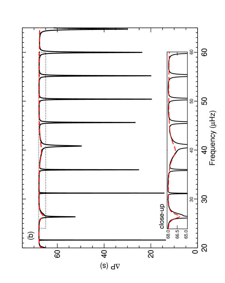
Figure 5.— Period spacing derived from the analytical approach for model 1a. The inset shows a close-up around $\Delta P_{\rm as}$ (dotted box). (a) case with mode coupling but no glitch, computed from expression (35). (b) case with mode coupling and glitch, computed from expression (38) (black) and case with glitch and no mode coupling, computed from expression (24) (red), adopting $r_{\star}=0.0221R$ and $A=1.65\times 10^{-3}R$.

The period spacing derived from expression (35) for our model 1a is shown in Figure 5a. The dips associated with the coupling to the p modes are equally spaced in frequency and located at the acoustic resonant (cyclic) frequencies ($\omega_{\rm a}/2\pi$). At these frequencies the denominator inside the arctan of (34) goes through zero and, as a consequence, $\varphi$ varies rapidly with frequency. The large derivative in frequency of $\varphi$ therefore makes $\mathcal{F}_{\rm C}$ large, producing the dips in the period spacing. This is in agreement with the discussions by Christensen-Dalsgaard (2012) and Mosser et al. (2012b) and with the period spacing derived from the analysis of real data for red-giant stars (e.g. Beck et al., 2011).

Next, we add the effect of the glitch. Following the same steps as in section 3.2 we find that the eigenvalue condition in the presence of mode coupling and a glitch is given by

$$\int_{r_{1}}^{r_{2}}K_{0}{\rm d}r=\pi\left(n-\frac{1}{2}\right)-\Phi-\varphi,$$ (36)

where $\Phi$ is now defined by the following system of equations,

$$\left\{\begin{array}[]{lll}B\cos\Phi&=&1-A\displaystyle\frac{LN_{0}^{\star}}{r_{\star}\omega}\sin\left(\int_{r_{\star}}^{r_{2}}K_{0}{\rm d}r+\frac{\pi}{4}+\varphi\right)\times\\ &&\cos\left(\int_{r_{\star}}^{r_{2}}K_{0}{\rm d}r+\frac{\pi}{4}+\varphi\right)\\ \\ B\sin\Phi&=&A\displaystyle\frac{LN_{0}^{\star}}{r_{\star}\omega}\sin^{2}\left(\int_{r_{\star}}^{r_{2}}K_{0}{\rm d}r+\frac{\pi}{4}+\varphi\right).\end{array}\right.$$ (37)

We emphasize that both $B$ and $\Phi$ now depend on $\varphi$. This is to be expected, since the effect of the glitch on the oscillations depends critically on the phase of the eigenfunction at the depth where the glitch is located, and that phase is influenced by the coupling. As a consequence, the relative deviation of the period spacings from the asymptotic value when both a glitch and mode coupling are present is different from what would be found by simply adding the deviations generated by the coupling and by the glitch separately. This fact can be readily seen in the period spacing derived from the eigenvalue condition (36), which has the form

$$\Delta P\approx\frac{\Delta P_{\rm as}}{1-\displaystyle\frac{\omega^{2}}{\omega_{\rm g}}\left[\frac{{\rm d}\Phi}{{\rm d}\omega}+\frac{{\rm d}\varphi}{{\rm d}\omega}\right]}\equiv\frac{\Delta P_{\rm as}}{1-\mathcal{F}_{\rm{G,C}}}.$$ (38)

As before, the deviation of the period spacing from its asymptotic value is reflected in the second term, $\mathcal{F}_{\rm{G,C}}$, present in the denominator of expression (38). Its dependence on the glitch parameters can be made explicit by solving the system of equations (37), from which we obtain

$$\mathcal{F}_{\rm{G,C}} =$$ (39)

$$\frac{\omega^{2}}{\omega_{\rm g}}\frac{{\rm d}\varphi}{{\rm d}\omega}\left\{1+\frac{ALN_{0}^{\star}}{r_{\star}\omega B^{2}}\left[\cos\left(2\frac{\omega_{\rm g}^{\star}}{\omega}+2\varphi\right)\right.\right.$$

$$\hskip 42.67912pt\left.\left.-\frac{ALN_{0}^{\star}}{r_{\star}\omega}\sin^{2}\left(\frac{\omega_{\rm g}^{\star}}{\omega}+\frac{\pi}{4}+\varphi\right)\right]\right\}$$

$$+\frac{ALN_{0}^{\star}}{r_{\star}\omega_{\rm g}B^{2}}\left\{\frac{\omega_{\rm g}^{\star}}{\omega}\cos\left(2\frac{\omega_{\rm g}^{\star}}{\omega}+2\varphi\right)\right.$$

$$\hskip 2.84544pt\left.+\left(1-\frac{ALN_{0}^{\star}\omega_{\rm g}^{\star}}{r_{\star}\omega^{2}}\right)\sin^{2}\left(\frac{\omega_{\rm g}^{\star}}{\omega}+\frac{\pi}{4}+\varphi\right)\right\},$$

where, $B^{2}$ is now given by

$$B^{2} = \left[1-\frac{ALN_{0}^{\star}}{2r_{\star}\omega}\cos\left(2\frac{\omega_{\rm g}^{\star}}{\omega}+2\varphi\right)\right]^{2}$$ (40)

$$\hskip 56.9055pt+\left[\frac{ALN_{0}^{\star}}{r_{\star}\omega}\sin^{2}\left(\frac{\omega_{\rm g}^{\star}}{\omega}+\frac{\pi}{4}+\varphi\right)\right]^{2}.$$

We see that $\mathcal{F}_{\rm{G,C}}$ has two terms, each marked by a set of curly brackets. If we assume there is no coupling, meaning that $\varphi$ is zero for all frequencies, the first term vanishes because ${\rm d}\varphi/{\rm d}\omega=0$, and the second term becomes equal to equation (26), hence reducing $\mathcal{F}_{\rm{G,C}}$ to $\mathcal{F}_{\rm G}$ as expected. If instead we assume there is no glitch, which translates to $A=0$, then the second term vanishes, and the first term becomes equal to $\mathcal{F}_{\rm{C}}$ defined in equation (35), reducing $\mathcal{F}_{\rm{G,C}}$ to $\mathcal{F}_{\rm{C}}$; again as one would expect. Finally, we consider that both coupling and glitch are present, but we look specifically at what happens at the acoustic resonance where the coupling dominates the expression for $\mathcal{F}_{\rm{G,C}}$. Here, the frequency derivative of $\varphi$ is very large, and hence the first term is generally much larger than the second. However, we still have the two extra $\cos$ and $\sin^{2}$ ‘glitch-induced’ terms within the first set of curly brackets compared to just $\mathcal{F}_{\rm{C}}$ ($=\omega^{2}/\omega_{\rm g}\,\,{\rm d}\varphi/{\rm d}\omega$). This shows that the mode coupling, and therefore also the dips located at the acoustic resonance frequencies, is influenced by the glitch.

The period spacing obtained from expression (38) is illustrated in Figure 5b. Comparing with Figure 5a, we see that the combined effect of the glitch and the coupling on the period spacing is predominantly a change in the depth of the dips at the acoustic resonant frequencies. Whenever a dip caused by the glitch coincides with a dip caused by the coupling with the p modes, the depth of the latter is reduced. But if a hump produced by the glitch coincides with the dip caused by the coupling, the depth of the dip increases. This behaviour is oposite to what would be found if the the combined effect were simply the sum of the deviations to the asymtotic period spacings caused by each effect separatly. The predicted behaviour can be understood if we recall that the extent to which g modes couple to a p mode depends critically on the proximity of their frequencies (assuming everything else remains unchanged, which is the case here). A glitch-induced dip in the period spacings means the g modes are locally more densely packed, as compared to the asymptotic case. Thus, if the dip coincides with an acoustic resonant frequency the number of g modes coupling to the p mode is greater, resulting in a wider and, consequently, shallower coupling dip. However, if an acoustic resonant frequency coincides with a glitch-induced hump, the number of g modes coupling to the p mode is reduced, resulting in a thinner, hence, deeper coupling dip.

4. Interpretation of full numerical solutions

In this section we consider the numerical solution of the full pulsation equations, including the perturbation to the gravitational potential, for the models introduced in section 2 and interpret them in the light of the results found with the toy model analysis presented in section 3. The full numerical solutions were computed with the pulsation code ADIPLS. Care was taken to have an adequate number of mesh points with appropriate distribution to resolve the rapidly varying eigenfunctions in the g-mode cavity.

The period spacing derived for our model 1a from the full numerical solutions is shown in Figure 6 (solid curve). Comparing with Figure 5 we see that the dips associated with the acoustic resonant frequencies are closer in frequency in the results from the full numerical solutions than in the toy model. This reflects the fact that the large separation computed from the eigenfrequencies is smaller (by about 5$\%$ in the current case) than the corresponding asymptotic value, in accordance with the results of previous studies (e.g. Stello et al., 2009; Belkacem et al., 2013; Mosser et al., 2013). Letting aside that difference, we see that in the full numerical solutions the dips associated with the acoustic resonant frequencies show a depth variation resembling what is seen using our toy model (Figure 5b). Comparison with the period spacing derived numerically considering only the g modes (section 3.2.3) (red, dashed curve in Figure 6) confirms that the glitch in the buoyancy frequency is the cause of the larger-scale modulation seen in the full solution (see inset), and, thus, that the combined effect of the glitch and mode coupling is to reduce/increase the depth of the dips positioned at the acoustic resonant frequencies when they coincide with a glitch-induced dip/hump.

Figure 6.— Period spacings derived from ADIPLS for model 1a, including the effects of the glitch and of the coupling between the g-modes and the p-modes (solid curve), compared to the integration of the wave equation (2), ignoring the coupling with p modes (red, dashed curve). The inset shows a close up around $\Delta P_{\rm as}$ (dotted box).

To illustrate how a glitch in the buoyancy frequency could be revealed in observational data, Figure 7 shows (a) $1/\sqrt{Q_{nl}}$ representative of relative mode amplitude (Christensen-Dalsgaard, 2004; Aerts et al., 2010), and both (b) a frequency- and (c) a period-échelle diagram corresponding to model 1a. Here, $Q_{nl}$ is a measure of the inertia of a mode of radial order $n$ and degree $l$, relative to that of radial modes defined by

$$Q_{nl}=\frac{{I}_{nl}}{\overline{{I}}_{l=0}},$$ (41)

where $I_{nl}$ is the surface normalized mode inertia,

$$I_{nl}=\frac{\int_{0}^{R_{\rm s}}\left[\xi_{\rm r}^{2}+l\left(l+1\right)\xi_{\rm h}^{2}\right]\rho r^{2}{\rm d}r}{M\xi_{\rm r}\left(R_{\rm s}\right)^{2}},$$ (42)

and $\overline{{I}}_{l=0}$ is obtained by interpolating ${I}_{n0}$ to the frequency of the mode under consideration. Moreover, $\xi_{\rm r}$ and $\xi_{\rm h}$ are the radial and horizontal components of the displacement, respectively, $M$ is the stellar mass, and $R_{\rm s}$ is the surface radius. The frequency échelle shows the frequency spectrum (Figure 7a) divided into segments of fixed length that are stacked one above the other. The length of segments equals the average frequency separation between overtone radial modes, $\Delta\nu$, found as the slope of a linear fit to the radial modes versus their order (Grec et al., 1983). In the period-échelle diagram we show only the dipole modes, and here the abscissa is the mode period modulo the asymptotic period spacing, $\Delta P_{\mathrm{as}}$(equation (18), see e.g., Bedding et al. (2011)). For clarity, we show only modes of relative amplitude above 5% of the radial modes in the échelle diagrams.

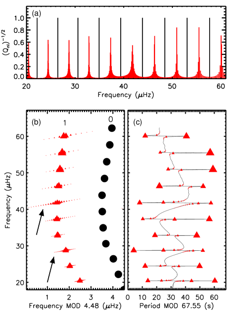
Figure 7.— Model 1a ($\nu_{\rm max}$ $=45\,$$\mu$Hz) - (a) Pseudo amplitude spectrum based purely on mode inertia relative to the radial modes ($1/\sqrt{Q_{nl}}$), (radial in black and dipole in red). (b) Échelle diagram including radial (circles) and dipole (triangles) modes. The abscissa is the frequency modulo $\Delta\nu$. Symbol size follows the peak heights from panel (a). The arrows indicate clusters of dipole modes affected by a glitch-induced dip in the period spacing. (c) Period échelle following the notation of panel (b). The abscissa is the period modulo $\Delta P_{\mathrm{as}}$. The solid curve connects all the dipole modes.

Noise set aside, the result seen in this model is a broadening of the clusters of ‘observable’ dipole modes where the location of the dips coincides with that of a cluster. We see this effect in Figure 7a near 28$\mu$Hz and 41$\mu$Hz (see also Figure 6). In the period-échelle diagram, the same effect shows as a strong distortion of the usual ‘S’ shaped mode pattern seen between each radial mode order in a glitch-free case (see for example figure 1 of Bedding et al. (2011)).

Next we consider the full numerical solutions for our model 1b, located in the core-helium-flash evolution phase. The period spacings derived from the ADIPLS results for this model are shown in Figure 8 (solid curve). The existence of closely-spaced pronounced dips in the period spacing makes it harder to identify the dips associated with the acoustic resonant frequencies in this case. To help with that identification, we mark the frequencies of the radial acoustic modes (vertical lines) and recall that the dips produced by the coupling between p and g dipole modes should be positioned roughly mid way between consecutive radial modes. Indeed, single or double dips of greater depth than their neighbors are found at the expected frequencies. Comparison of the period spacing derived from the full solutions (solid curve) with that derived considering only the g modes (red, dashed curve) shows that the two are similar everywhere, except at the frequencies of these more pronounced dips. This confirms that the more pronounce dips are produced by the coupling between the p and g modes and excludes that this coupling is the cause for the other dips. Using our analytical model for the case of having a glitch but no coupling (equation (24)) we find that the less pronounced dips are caused by the outer spike in the buoyancy frequency (Figure 2b), that is, the glitch at the hydrogen-burning shell. Moreover, we also confirm, based on the analytical model, that despite the glitch being located relatively far from the center of the cavity (at $\omega_{\rm g}^{\star}/\omega_{\rm g}=0.075$) the larger-scale modulation seen in the period spacing (on a scale of about 10 glitch-induced dips) is explained by the sampling effect discussed in section 3.2.2.

The separation between glitch-induced dips in model 1b is similar to the width of the dips associated with the acoustic resonant frequencies, which makes it difficult to interpret the combined effect of the glitch and the mode coupling in this case. Nevertheless, the comparison between the dips at $\approx 18.1\mu{\rm Hz}$ and $23.2\mu{\rm Hz}$, indicates that the combined effect is the same as for model 1a. The latter dip is placed at a glitch-induced hump and, consequently, has its depth increased, while the former dip is placed at a glitch-induced dip and has its central depth reduced, forming a double-dip structure. The observational impact of these double-dip structures will be discussed in section 5.

Figure 8.— Period spacings derived from ADIPLS for model 1b, including the effects of the glitch and of the coupling between the g-modes and the p-modes (solid curve), compared to the integration of the wave equation (2), ignoring the coupling with p modes (red, dashed curve). The vertical, lines indicate the frequencies of the radial modes.

5. Observing glitches in red giants

Next, we search an extensive set of stellar models of various masses to locate the stages of evolution where one could potentially observe the seismic signature from buoyancy glitches in red giants. Our stellar models are derived using the ‘default’ work inlist of MESA-v5271 (Paxton et al., 2011, 2013) with the only change that we turned off mass loss. These canonical models do not include diffusion or extra mixing beyond convection defined by the classical Schwarzschild criterion (Schwarzschild, 1906). Our search comprises tracks ranging 1.0-3.0M_⊙, all roughly with solar abundance, spanning the entire evolution from the bottom of the red-giant branch to near the end of the asymptotic-giant branch. To check that we obtain consistent results we also derived ASTEC tracks for 1.0M_⊙ to near the tip of the red-giant branch and for 2.4M_⊙ to the end of helium-core burning. The frequency calculations based on the full numerical solution shown in this section were made using GYRE (Townsend & Teitler, 2013), but spot checks were made to verify that these results were consistent with what we obtained using ADIPLS.

For each model, we calculate the dipole g-mode frequencies by solving equation (2) numerically, with $K$ defined by equation (31) as described in section 3.2.3; hence, neglecting the coupling to the acoustic cavity. The calculation is restricted to within a $\nu_{\rm max}$/2-wide range centered around the solar-scaled $\nu_{\rm max}$$\propto g/\sqrt{T_{\mathrm{eff}}}$, where $T_{\mathrm{eff}}$ is the effective temperature and $\nu_{\rm max}$ is the frequency of maximum oscillations power. This range is roughly equal to the full width at half maximum of the excess power observed for solar-like oscillations (Stello et al., 2004; Kjeldsen et al., 2005; Mosser et al., 2012a). From the resulting frequencies we then derive the series of pairwise period spacings, $\Delta P$, and calculate an index of glitch-induced variation in $\Delta P$ to determine if the g-modes are effected by a glitch. We tested two indices, both showing consistent results. One was simply the RMS of the period spacings and the other was the height of the strongest peak in the Fourier transform of the series of period spacings versus period. The latter is shown for a section of the 1M_⊙ track in Figure 9(a) indicating a region bracketed by the vertical dotted lines where the index is above twice the floor level. This phase is therefore identified as showing excess variation in $\Delta P$. Following the approach described in relation to Figure 7b (section 4), we also derive the large frequency separation for radial modes, $\Delta\nu$.

5.1. Before helium ignition

Along the red giant branch we find glitch-induced variations only at one particular phase in evolution lasting roughly 5-10 million years. Interestingly, this coincides with the luminosity bump.

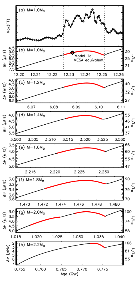
Figure 9.— Panel (a): Maximum signal in the Fourier transform of the series of period spacings along the 1M_⊙ track. Vertical dotted lines bracket the region of glitch-induced variation in $\Delta P$. Panels (b-h): Close-up of the evolution near the red giant branch luminosity bump as a function of age for models with fully or partially-degenerate cores. Thick red curves indicate phases of excess variation in $\Delta P$. A MESA- equivalent of model 1a discussed in sections 2-4 is shown, in panels (a) and (b).

Figure 9(b-h) summarizes the results near the bump for low-mass models ($1.0\leq M\leq 2.2\mathrm{M}_{\odot}$). Models beyond $2.2\mathrm{M}_{\odot}$ do not show the bump because the glitch from the first dredge-up is not reached by the hydrogen-burning shell until after the model is past the tip of the red-giant branch. The thick red curves indicate the phases of excess variation in $\Delta P$. This excess variation can be attributed to the glitch left by the dredge-up as illustrated by model 1a (Figure 9b). The only exception to this picture is along the 2.0M_⊙ track, which shows an extra slightly earlier phase of excess variation arising from a subtle but interesting combination of effects, also resulting in the extra luminosity bump we see for this mass at 1.026 Gyr. During the main-sequence phase the gradually retreating convective core leaves a steep gradient in molecular weight (hence a spike in the buoyancy frequency) where the convection reached its maximal extent at young age. For models below 1.8M_⊙, the gradient is smoothed away by the hydrogen-burning shell, which is later established at almost the same location. However, for models of roughly 2.0M_⊙, the hydrogen-burning shell starts at a smaller radius relative to this gradient, and the gradient therefore survives for a while. This allows the star to evolve to the point where the local wavelength becomes comparable to the scale of the associated spike in the buoyancy frequency, giving rise to the first phase of excess variation in $\Delta P$ that ends when the hydrogen-burning shell finally reaches the location of the spike. In more massive stars that same spike is erased by the first dredge-up before the spike appears as a glitch for the gravity waves.

5.2. After helium ignition

Figure 10.— Early (left) and late (right) stages of helium core burning. Thick red curves indicate phases of excess variation in $\Delta P$. The time in Myrs since helium ignition at the tip of the red giant branch is indicated along the top axis of each panel. Down/Up-ward pointing arrows show the start/end of quiescent helium-core burning (see text). The left- and right-side annotation of the ordinate applies to both panels.

In Figure 10 we show the result for post-helium ignition tracks with masses 1.0M_⊙, 1.6M_⊙, 2.2M_⊙, and 2.8M_⊙. Again, thick red curves indicate evolution phases showing excess variation in $\Delta P$. The downward-pointing arrows indicate when the last off-center helium sub-flash and associated convection zone reaches the center, signifying the start of quiescent helium-core burning in the models with degenerate cores before helium ignition (Figure 10a,c). There is no such equivalent for the higher-mass models, in which a more gentle at-center helium ignition starts immediately at the tip of the red giant branch. The upward-pointing arrows mark the end of helium-core burning at the so-called asymptotic-giant-branch bump, and the subsequent asymptotic-giant-branch phase. In the following we will discuss each phase in turn where we see excess variation in $\Delta P$.

5.2.1 Low-mass stars

Along the 1.0M_⊙ track we see repeated intervals of excess variation during the initial helium sub-flashing phase. Each of these intervals are interspersed by short off-center helium burning sub-flashes where the g-mode cavity is split in two (Bildsten et al., 2012). If both g-mode cavities are taken into account, the resulting effect on $\Delta P$ during this cavity split differs significantly from what is presented by Bildsten et al. (2012), who ignored the inner cavity in their analysis. The results including both cavities will be discussed in a forthcoming paper. The intervals with only one g-mode cavity are illustrated by model 1b, discussed in sections 2-4, and model 2 (Figure 10a). In Figure 11 we show a multi-faceted view of model 2 including its core structure and the glitch effect on the observed frequencies.

Figure 11.— Model 2 ($M=1.0$ M_⊙ ; $\nu_{\rm max}$$=31\,$$\mu$Hz) - (a) Buoyancy frequency with key features indicated. (b) Period spacing of pure g modes (as in section 3.2.2) (red) and full numerical solution using GYRE (black). The vertical dotted lines indicate the approximate position of the dipole acoustic modes. They have been positioned relative to the nearest radial mode in agreement with Stello et al. (2014) (see also Huber et al. (2010); Montalbán et al. (2010)). Horizontal dotted line marks $\Delta P_{\mathrm{as}}$. (c) Pseudo amplitude spectrum based purely on mode inertia, normalized to the radial modes. Dipole modes are shown in red and radial modes in black. (d) Échelle diagram. The abscissa is the frequency modulo $\Delta\nu$. Symbol size follows the peak heights in panel (c). (e) Period échelle diagram. Symbol sizes as in panel (d). The abscissa is the period modulo $\Delta P_{\mathrm{as}}$. Dotted lines indicate the approximate position of the dipole acoustic modes. Black curve connects all dipole modes.

Model 2 is similar to model 1b except that it has a lower luminosity, hence larger $\nu_{\rm max}$  and is therefore more likely to represent a case where $\Delta P$ can be measured in observational data (Mosser et al., 2014; Grosjean et al., 2014). As in model 1b, we see a series of glitch-induced dips in $\Delta P$ (Figure 11b). The associated dips in mode inertia, or peaks in amplitude (Figure 11c), suggest that some modes would be observable even if they are far from the acoustic resonant frequency. This decrease in the inertia arises because some, almost pure, g-modes are trapped in the outer part of the g-mode cavity. As a result, we see a split of the $l=1$ ridge in the échelle diagram (Figure 11d). That split is most evident where one of the glitch-induced dips coincides with an acoustic resonant frequency (a coupling-induced dip), splitting the coupling dip into two (Figure 11b).

In the following quiescent helium-core burning phase we see no significant variation in $\Delta P$ for our canonical models. However, towards the end of core burning (Figure 10b), the retreating convective core leaves a sharp glitch, which results in very high-frequency variation in $\Delta P$ at the asymptotic-giant-branch bump and the early helium-shell burning phase. Figure 12 shows the buoyancy frequency of model 3, which is representative for models in this phase. The glitch is located closely to the center of the cavity (at $\omega_{\rm g}^{\star}/\omega_{\rm g}\sim 0.5$). Hence, the induced period-spacing variations occur over a scale comparable to the separation between two consecutive modes, which results in a low-frequency modulation in $\Delta P$ on top of the high-frequency variation, as discussed in section 3.2.2 and illustrated by the analytical result in Figure 4c. The numerical result including adiabatic frequencies and inertias of such models is still under investigation and will be presented in a forthcoming paper.

Figure 12.— Model 3 ($M=1.0$ M_⊙ ; $\nu_{\rm max}$$=15\,$$\mu$Hz) - Buoyancy frequency with key features indicated.

The $\Delta P$ variations indicated at the early helium-shell burning phase (Figure 10b, d, f, h) are similar for all masses that we investigated, and originate from the same physical reasons as discussed above for model 3. Moreover, all models that ignite helium in a degenerate core, which include the models shown in Figure 10c, show quite similar behavior to the 1.0M_⊙ case, and will not be discussed further.

5.2.2 High-mass stars

Moving on to a case where helium ignites in a partially degenerate core, we see excess variation in the early stages of helium core burning as illustrated along the 2.2M_⊙ track (Figure 10e). This variation originates from the glitch at the hydrogen-burning shell. We show a representative model in Figure 13.

Figure 13.— Model 4 ($M=2.2$ M_⊙ ; $\nu_{\rm max}$$=84\,$$\mu$Hz) - notation as in Figure 11.

Finally, representative of stars igniting helium in a non-degenerate core, the 2.8M_⊙ track shows two phases of excess variation during early stages of helium-core burning (Figure 10g). The first phase is the ‘high-mass’ non-degenerate-core equivalent to what we saw in the low-mass degenerate-core models near the red-giant-branch bump, where the glitch from the first dredge-up ‘enters’ the g-mode cavity (Figures 9 and 1c). As in the red-giant-branch bump cases, the $\Delta P$ variation vanishes when the hydrogen-burning shell reaches and smooths out the glitch, but here this occurs after the model has become a quiescent helium-core burning clump star with $\Delta\nu$ $\sim\,7.5\,$$\mu$Hz. Figures 14, 15, and 16 show three examples along this phase of evolution.

Figure 14.— Model 5 ($M=2.8$ M_⊙ ; $\nu_{\rm max}$$=34\,$$\mu$Hz) - notation as in Figure 11.

Figure 15.— Model 6 ($M=2.8$ M_⊙ ; $\nu_{\rm max}$$=65\,$$\mu$Hz) - notation as in Figure 11.

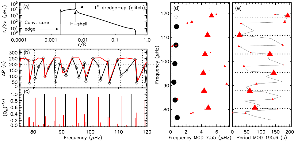
Figure 16.— Model 7 ($M=2.8$ M_⊙ ; $\nu_{\rm max}$$=100\,$$\mu$Hz) - notation as in Figure 11.

Like in model 2, the glitch in these three models is expected to cause relative high amplitudes in the frequency spectrum for the almost pure g modes located at dips in $\Delta P$ (panels b and c). The échelle diagram can therefore appear to show a dominant spacing between strong modes that is significantly larger than the underlying period spacing between adjacent modes (Figure 15d). A second phase of variation occurs due to a glitch that was built up near the edge of the convective core during helium ignition and its subsequent maximal extent. However, we do not show an example of this phase because, in our models, the variation only shows up with a relatively low amplitude ($\Delta P$ $\sim 10\,$ sec) and dips in $\Delta P$ that are rather broad and widely separated, making it very difficult to detect when the coupling to the acoustic modes is included.

5.3. Discussion

Due to the glitch-induced variation in $\Delta P$ around $\Delta P_{\mathrm{as}}$, one can choose to use either $\Delta P_{\mathrm{as}}$ (horizontal dotted line in panel b) or the maximum period spacing to generate the period échelle (see for example Figure 15b). We chose to use $\Delta P_{\mathrm{as}}$, which in some cases creates one overall ‘S’ shape per radial mode order as in the glitch-free case (see high-frequency end of Figure 7; see also Fig.1c of Bedding et al. (2011)), but modulated with the glitch-induced variation on top as in Figure 11e and  13e. Had we chosen to use the maximum value of $\Delta P$, we would obtain one ‘S’ shape for every glitch-induced dip in $\Delta P$. In other cases using $\Delta P_{\mathrm{as}}$ makes the period échelle look very complicated with no clear pattern, such as in Figures 14e, while the maximum value appears to create a better aligned échelle, by straightening the zig-zag pattern. The latter might therefore be misinterpreted as the asymptotic period spacing of a glitch-free star. This could potentially explain some of the more massive stars with observed $\Delta P_{\mathrm{as}}$ reported to fall significantly outside the main ensemble in the $\Delta P_{\mathrm{as}}$-$\Delta\nu$ diagram by Mosser et al. (2014), if indeed real stars share the frequency behavior shown by our models.

In search for excess variation in $\Delta P$, as summarized in Figures 9 and 10, we deliberately ignored the coupling with the envelope (p-)modes to simplify and speedup the process. In real data, one would have to separate the variation in $\Delta P$ caused by the coupling from the effect induced by the buoyancy glitches. We verified that our results presented here are consistent with what we obtain if the p-mode coupling is included, which we did by first fitting and removing the coupling pattern from the mixed-mode frequencies derived from the full numerical solution (e.g. ADIPLS/GYRE), and subsequently deriving the RMS of the residual period-spacing variation. Fitting and removing the coupling pattern was performed along 1.0M_⊙ and 2.4M_⊙ tracks using the toy model for the coupling presented by Stello (2012), but could as well be done using equation (35) (see also equation (9) in Mosser et al., 2012b). The analysis of glitch-induced variations in $\Delta P$ from real data will be presented in Stello et al. (in preparation).

Although we verified that the results summarized in Figures 9 and 10 are similar when based on ASTEC, our ASTEC models generally showed less high-frequency variation in $\Delta P$ due to the glitches being smoother, arising from numerical diffusion in ASTEC, as described in section 2. It is also expected that including additional mixing processes could affect the buoyancy frequency significantly, and hence alter the signature in the frequencies, which would potentially provide a way to test various prescriptions of mixing (Constantino et al., in preparation).

6. Conclusions

We have shown that structural glitches in the cores of red giants can significantly affect the adiabatic properties of their mixed modes – both mode inertias and frequencies. The modulation in mode inertia can have strong consequences for which modes are observable. Moreover, the change in the frequency pattern shows up as a variation in the underlying period spacing of pure g-modes around the fixed asymptotic value of the glitch-free case. Hence, assuming the period spacing follows the simple glitch-free asymptotic behavior (equation (35), see also equation (9) in Mosser et al. (2012b)), can hamper the estimate of the asymptotic (glitch-free) period spacing, $\Delta P_{\mathrm{as}}$. This might explain some of the stars observed to show a period spacing that does not follow the main ensemble of stars both along the red-giant branch and the red clump (Mosser et al., 2014).

We provide an approximate analytical solution to the wave equation in the presence of both a structural glitch and the coupling between p and g modes. We find that the combined effect of a glitch and mode coupling is not merely the sum of the two. The combined effect is a modulation of the depth of the dips at the acoustic resonant frequencies and, in some cases, the split of these in two. The glitch-induced variations in the period spacing are equally spaced in period, and reflect the depth at which the glitch is located, while the amplitude of the variation is a measure of the effective strength of the glitch.

From an extensive set of evolution tracks of varying mass we find glitch-induced variation at the red-giant-branch luminosity bump, at the early phases of helium-core burning, and at the asymptotic-giant-branch bump, which signifies the beginning of helium shell burning. We note that some of these evolution stages last for a relatively short period of time, making the detection of glitches in such stars a strong indicator of relative age.

Appendix A

In this appendix we derive the explicit form of the coupling phase, $\varphi$, that appears in equation (33). This phase is uniquely determined by the coefficients entering the solution of the wave equation in the evanescent region $r_{2}\ll r\ll r_{3}$. In principle these can be determined by matching the solution in the evanescent region to that in the p-mode cavity and, subsequently, applying an appropriate boundary condition at the photosphere. However, in red-giant models such as those under study, we find that $K^{2}$ defined by equation (3) goes to $-\infty$ at some critical radius $r_{\rm c}$ located in the evanescent region between the two cavities. The analysis of the wave equation across this singularity is rather cumbersome and will be considered in a separate paper (Cunha et al., in preparation). Here, we use, instead, the eigenvalue condition presented by Shibahashi (1979), which accounts for mode coupling but not for rapid variations in the structure (hence no glitch). Their eigenvalue condition is derived through the asymptotic analysis of the pulsation equations, under the Cowling approximation, for two pulsation variables, one related to the radial component of the displacement and the other related to the Eulerian pressure perturbation. The simultaneous use of the two equations allows the author to avoid having to match the solutions across critical points similar to that referred above. The result is the eigenvalue condition (Shibahashi, 1979, equation (31))

$$\cot\left(\int_{r_{1}}^{r_{2}}\kappa_{0}{\rm d}r\right)\tan\left(\int_{r_{3}}^{r_{4}}\kappa_{0}{\rm d}r\right)=q$$ (43)

where $q$ is often called the coupling factor and is given by

$$q=\frac{1}{4}\exp\left({-2\int_{r_{2}}^{r_{3}}\mid\kappa_{0}\mid{\rm d}r}\right),$$ (44)

where, as before, we used the subscript 0 to indicate that this condition is valid in the absence of a glitch. In the above, $\kappa_{0}$ is an approximation to the radial wavenumber appearing in the equations used by the author and is given by

$$\kappa_{0}^{2}=\frac{\omega^{2}-N_{0}^{2}}{c^{2}}-\frac{L^{2}}{r^{2}}\left(1-\frac{N_{0}^{2}}{\omega^{2}}\right).$$ (45)

Inside the g-mode cavity $\kappa_{0}\approx L/r\,\sqrt{(1-N_{0}^{2}/\omega^{2})}\approx K_{0}$. Using this fact, we can combine the conditions (33) and (43) to write,

$$\tan\left(\varphi\right)=\frac{q}{\tan\left(\int_{r_{3}}^{r_{4}}\kappa_{0}{\rm d}r\right)}.$$ (46)

Next, we note that the eigenvalue condition for pure p modes derived by Shibahashi (1979) (his equation (26)) is

$$\int_{r_{3}}^{r_{4}}\kappa_{0{\rm a}}=m\pi,$$ (47)

where $m$ is an integer and the subscript “a” was added to indicate that this condition provides what would be the eigenfrequencies of acoustic waves in the absence of coupling.

Writing $\kappa_{0}\equiv\kappa_{0{\rm a}}+\delta\kappa$ and taking $\delta\kappa\approx\delta\omega/c$ (which is a good approximation throughout the p-mode cavity, except near the turning points $r_{3}$ and $r_{4}$) we then have

$$\tan\left(\int_{r_{3}}^{r_{4}}\kappa_{0}{\rm d}r\right) = \tan\left(m\pi+\int_{r_{3}}^{r_{4}}\delta\kappa{\rm d}r\right)$$ (48)

$$\approx \tan\left(\frac{\omega-\omega_{\rm a}}{\omega_{\rm p}}\right),$$

where $\omega_{\rm a}$ are the eigenvalues that would be obtain for p modes in the absence of coupling and $\omega_{\rm p}^{-1}=\int_{r_{3}}^{r_{4}}c^{-1}{\rm d}r$. Finally, using (48) in equation (46) we find

$$\varphi\approx{\rm atan}\left[\frac{q}{\tan\left(\displaystyle\frac{\omega-\omega_{\rm a}}{\omega_{\rm p}}\right)}\right].$$ (49)

Appendix B

Below we reproduce the expressions for the generalized buoyancy frequency and critical frequency that appear in equations (5.4.8) and (5.4.9) derived by Gough (1993).

In Gough (1993), the author expresses the equations describing linear, adiabatic pulsations in terms of the Lagrangian pressure perturbation $\delta p$. After performing the Cowling approximation, the resulting second order differential equation for $\delta p$ is reduced to the standard form by defining a new dependent variable $\Psi=~{}(r^{3}/g\rho f)^{1/2}\delta p$, where $f$ is the f-mode discriminant given by

$$f=\frac{\omega^{2}r}{g}+2+\frac{r}{H_{\rm g}}-\frac{L^{2}g}{\omega^{2}r},$$ (50)

and $H_{g}$ is the scale height for the gravitational acceleration obtained following the general definition adopted by the author that the scale height for a quantity $q$ is $H_{q}=-\frac{{\rm d}r}{{\rm d}\ln q}$. The wave equation resulting from this variable transformation is

$$\frac{{\rm d}^{2}\Psi}{{\rm d}r^{2}}+K^{2}\Psi=0,$$ (51)

with the radial wavenumber $K$ defined by,

$$K^{2}=\frac{\omega^{2}-\omega_{\rm c}^{2}}{c^{2}}-\frac{L^{2}}{r^{2}}\left(1-\frac{\mathcal{N}^{2}}{\omega^{2}}\right).$$ (52)

In the above, $\mathcal{N}$ is the generalized buoyancy frequency given by

$$\mathcal{N}^{2}=g\left(\frac{1}{\mathcal{H}}-\frac{g}{c^{2}}-\frac{2}{h}\right),$$ (53)

where $h$ is the scale height for $g/r^{2}$ and is related to $H_{g}$ by $h^{-1}=H_{g}^{-1}+2r^{-1}$ and $\mathcal{H}$ is the scale height for $g\rho f/r^{3}$ and is related to other relevant scale heights in the analysis by $\mathcal{H}^{-1}=H_{\rho}^{-1}+H_{f}^{-1}+h^{-1}+r^{-1}$. Moreover, $\omega_{c}$ is a generalization of the critical frequency given by

$$\omega_{c}^{2}=\frac{c^{2}}{4\mathcal{H}^{2}}\left(1-2\frac{{\rm d}\mathcal{H}}{{\rm d}r}\right)-\frac{g}{h}$$ (54)

Using the definition for the density scale height and the equation for hydrostatic equilibrium, the buoyancy frequency defined by expression  (1) can be written as,

$$N^{2}=g\left(\frac{1}{H_{\rho}}-\frac{g}{c^{2}}\right).$$ (55)

Comparing this expression with expression (53) we see that the generalized buoyancy frequency has $\mathcal{H}$ in the place of $H_{\rho}$ and includes an additional term, $-2/h$. As mentioned by Gough (1993) (and seen from the definitions of $h$ and $\mathcal{H}$), these differences result from the geometry and self-gravity of the equilibrium state and, consequently, $\mathcal{N}^{2}$ reduces to $N^{2}$ in the limit of a plane-parallel envelope under constant gravitational acceleration. Comparison of the generalized critical frequency with the one derived in that same limit (Gough, 2007), shows that the difference between the two is also solely the outcome of geometry and self-gravity.

References

- Aerts et al. (2010) Aerts, C., Christensen-Dalsgaard, J., & Kurtz, D. W. 2010, Asteroseismology (Springer)
- Beck et al. (2011) Beck, P. G., et al. 2011, Science, 332, 205
- Beck et al. (2012) —. 2012, Nature, 481, 55
- Bedding et al. (2010) Bedding, T. R., et al. 2010, ApJ, 713, L176
- Bedding et al. (2011) —. 2011, Nature, 471, 608
- Belkacem et al. (2013) Belkacem, K., Samadi, R., Mosser, B., Goupil, M.-J., & Ludwig, H.-G. 2013, in Astronomical Society of the Pacific Conference Series, Vol. 479, Progress in Physics of the Sun and Stars: A New Era in Helio- and Asteroseismology, ed. H. Shibahashi & A. E. Lynas-Gray, 61
- Bildsten et al. (2012) Bildsten, L., Paxton, B., Moore, K., & Macias, P. J. 2012, ApJ, 744, L6
- Brassard et al. (1992) Brassard, P., Fontaine, G., Wesemael, F., & Hansen, C. J. 1992, ApJS, 80, 369
- Broomhall et al. (2014) Broomhall, A.-M., et al. 2014, MNRAS, 440, 1828
- Cantiello et al. (2014) Cantiello, M., Mankovich, C., Bildsten, L., Christensen-Dalsgaard, J., & Paxton, B. 2014, ApJ, 788, 93
- Charpinet et al. (2000) Charpinet, S., Fontaine, G., Brassard, P., & Dorman, B. 2000, ApJS, 131, 223
- Christensen-Dalsgaard (2004) Christensen-Dalsgaard, J. 2004, Sol. Phys., 220, 137
- Christensen-Dalsgaard (2008a) —. 2008a, Ap&SS, 316, 113
- Christensen-Dalsgaard (2008b) —. 2008b, Ap&SS, 316, 13
- Christensen-Dalsgaard (2012) Christensen-Dalsgaard, J. 2012, in Astronomical Society of the Pacific Conference Series, Vol. 462, Progress in Solar/Stellar Physics with Helio- and Asteroseismology, ed. H. Shibahashi, M. Takata, & A. E. Lynas-Gray, 503
- Cunha & Brandão (2011) Cunha, M. S., & Brandão, I. M. 2011, A&A, 529, A10
- Cunha & Metcalfe (2007) Cunha, M. S., & Metcalfe, T. S. 2007, ApJ, 666, 413
- Degroote et al. (2010) Degroote, P., et al. 2010, Nature, 464, 259
- Dupret et al. (2009) Dupret, M.-A., et al. 2009, A&A, 506, 57
- Frandsen et al. (2002) Frandsen, S., et al. 2002, A&A, 394, L5
- Gough (1993) Gough, D. O. 1993, in Astrophysical Fluid Dynamics - Les Houches 1987, ed. J.-P. Zahn & J. Zinn-Justin, 399–560
- Gough (2007) Gough, D. O. 2007, Astronomische Nachrichten, 328, 273
- Grec et al. (1983) Grec, G., Fossat, E., & Pomerantz, M. A. 1983, Sol. Phys., 82, 55
- Grosjean et al. (2014) Grosjean, M., Dupret, M.-A., Belkacem, K., Montalban, J., Samadi, R., & Mosser, B. 2014, A&A, 572, A11
- Houdek & Gough (2007) Houdek, G., & Gough, D. O. 2007, MNRAS, 375, 861
- Huber et al. (2010) Huber, D., et al. 2010, ApJ, 723, 1607
- Kjeldsen et al. (2005) Kjeldsen, H., et al. 2005, ApJ, 635, 1281
- Mazumdar et al. (2014) Mazumdar, A., et al. 2014, ApJ, 782, 18
- Miglio et al. (2008) Miglio, A., Montalbán, J., Noels, A., & Eggenberger, P. 2008, MNRAS, 386, 1487
- Miglio et al. (2010) Miglio, A., et al. 2010, A&A, 520, L6
- Montalbán et al. (2010) Montalbán, J., Miglio, A., Noels, A., Scuflaire, R., & Ventura, P. 2010, ApJ, 721, L182
- Monteiro et al. (2000) Monteiro, M. J. P. F. G., Christensen-Dalsgaard, J., & Thompson, M. J. 2000, MNRAS, 316, 165
- Monteiro & Thompson (2005) Monteiro, M. J. P. F. G., & Thompson, M. J. 2005, MNRAS, 361, 1187
- Montgomery et al. (2003) Montgomery, M. H., Metcalfe, T. S., & Winget, D. E. 2003, MNRAS, 344, 657
- Mosser et al. (2012a) Mosser, B., et al. 2012a, A&A, 537, A30
- Mosser et al. (2012b) —. 2012b, A&A, 540, A143
- Mosser et al. (2012c) —. 2012c, A&A, 548, A10
- Mosser et al. (2013) —. 2013, A&A, 550, A126
- Mosser et al. (2014) —. 2014, ArXiv e-prints
- Østensen et al. (2014) Østensen, R. H., Telting, J. H., Reed, M. D., Baran, A. S., Nemeth, P., & Kiaeerad, F. 2014, ArXiv e-prints
- Paxton et al. (2011) Paxton, B., Bildsten, L., Dotter, A., Herwig, F., Lesaffre, P., & Timmes, F. 2011, ApJS, 192, 3
- Paxton et al. (2013) Paxton, B., et al. 2013, ApJS, 208, 4
- Roxburgh & Vorontsov (2001) Roxburgh, I. W., & Vorontsov, S. V. 2001, MNRAS, 322, 85
- Salaris et al. (2002) Salaris, M., Cassisi, S., & Weiss, A. 2002, PASP, 114, 375
- Schwarzschild (1906) Schwarzschild, K. 1906, Nachrichten von der Königlichen Gesellschaft der Wissenschaften zu Göttingen. Math.-phys. Klasse, 195, 41
- Shibahashi (1979) Shibahashi, H. 1979, PASJ, 31, 87
- Stello (2012) Stello, D. 2012, in Astronomical Society of the Pacific Conference Series, Vol. 462, Progress in Solar/Stellar Physics with Helio- and Asteroseismology, ed. H. Shibahashi, M. Takata, & A. E. Lynas-Gray, 200
- Stello et al. (2009) Stello, D., Chaplin, W. J., Basu, S., Elsworth, Y., & Bedding, T. R. 2009, MNRAS, 400, L80
- Stello et al. (2004) Stello, D., Kjeldsen, H., Bedding, T. R., De Ridder, J., Aerts, C., Carrier, F., & Frandsen, S. 2004, Sol. Phys., 220, 207
- Stello et al. (2014) Stello, D., et al. 2014, ApJ, 788, L10
- Tassoul (1980) Tassoul, M. 1980, ApJS, 43, 469
- Townsend & Teitler (2013) Townsend, R. H. D., & Teitler, S. A. 2013, MNRAS, 435, 3406
- Unno et al. (1989) Unno, W., Osaki, Y., Ando, H., Saio, H., & Shibahashi, H. 1989, Nonradial oscillations of stars (University of Tokyo Press)
- Winget et al. (1991) Winget, D. E., et al. 1991, ApJ, 378, 326