Analytic solutions for the Burgers equation with source terms

Abstract.

Analytic solutions for Burgers equations with source terms, possibly stiff, represent an important element to assess numerical schemes. Here we present a procedure, based on the characteristic technique to obtain analytic solutions for these equations with smooth initial conditions.

1. Introduction

Exact solutions of hyperbolic balance laws are very useful to assess the performance of numerical schemes. Non-linearity of partial differential equation, as well as, stiffness of source terms are desirable features to be recovered by numerical schemes. The analytic solutions presented here contain these elements.

Exact solutions for Burgers equations are generally obtained by separation of variables [1], regularization techniques [3], expansion methods [5], to mention but a few. Here, the strategy to solve these equations is based on the characteristic curve method, see [4, 2]. The solution is obtained in two steps. First, the solution of an Ordinary Differential Equation (ODE) called here, equivalent ODE, is obtained. This ODE is constructed by following the conventional characteristic curve method and contains the influence of the source term. Second, the solution of an ODE, called here characteristic ODE is obtained. This equation is defined in the $x-t$ plane and the solution of the equivalent ODE is included. In this way the influence of the source term is present in the definition of the characteristic curve.

To ensure the solvableness of the equivalent ODE, the existence of a primitive function for the reciprocal of the source term is required. Subsequently, if the solution of the equivalent ODE has a primitive function then the characteristic ODE is solvable. If these requirements are satisfied, analytic solutions can be obtained. However, a non-linear algebraic equation has to be solved in the general case, which require the initial condition to be a continuous function.

This work is organized as follows. In section 2 the procedure is presented. In section 3, the procedure is applied to the homogeneous Burgers equation. In section 4 the solution for a linear source term is obtained. In section 5 the analytic solution for a quadratic source term is obtained. In section 6, the methodology is applied to solve Burgers’s equation with a more general non-linear source term. Finally, in section 7 the main results of this work are summarized.

2. Analytic solutions for Burgers equations with a special class of source terms

To start, let us consider a balance law in the form

(3) $$\left.\begin{array}[]{c}\partial_{t}q(x,t)+\partial_{x}\biggl{(}\frac{q(x,t)^{2}}{2}\biggr{)}=s(q(x,t))\;,\\ q(x,0)=h_{0}(x)\;,\end{array}\right\}$$

where $h_{0}(x)$ is a continuous initial condition and $s(q)$ is the source term which has to satisfy the properties of lemma 2.2 shown below.

By following the characteristic curve method we define a curve $x$ in the $x-t$ plane, which satisfies

(6) $$\left.\begin{array}[]{c}\frac{d}{dt}x(t)=q(x(t),t)\;,\\ x(0)=y\;,\end{array}\right\}$$

with $y$ a constant value. This ODE will receive the name of characteristic ODE. On the other hand, we define

(7) $$\hat{q}(t)=q(x(t),t)\;,h(0):=q(x(0),0)=h_{0}(y)\;,$$

where $y$ is that given in (6). With these definitions, (3) becomes an ODE given by

(10) $$\left.\begin{array}[]{c}\frac{d}{dt}\hat{q}(t)=s(\hat{q}(t))\;,\\ \hat{q}(0)=h(0)\;.\end{array}\right\}$$

This ODE is called here, equivalent ODE.

Now, let us see the following definition in order to call for ensuring the existence of solutions.

Definition 2.1.

The primitive of a function $f(x)$ is a differentiable function $F(x)$ such that

(11) $$\frac{d}{dx}F(x)=f(x)\;.$$

Next lemma sets the type of source terms which are considered in this work.

Lemma 2.2.

If $s(\hat{q})^{-1}$ contains a primitive with respect to $\hat{q}$, then the equivalent ODE is solvable. Additionally, there exists a function $\mathcal{E}(t,h(0))$ such that

(14) $$\left.\begin{array}[]{c}\frac{\partial}{\partial t}\mathcal{E}(t,h(0))=s(\hat{q}(t))\;,\\ \mathcal{E}(0,h(0))=h(0)\\ \end{array}\right\}$$

and $\hat{q}(t)=\mathcal{E}(t,h(0))\;.$

Proof.

We integrate (6) as follows

(15) $$\int_{h(0)}^{\hat{q}(t)}s(q)^{-1}dq=\int_{0}^{t}dt\;,$$

as $s(q)^{-1}$ has a primitive function, there exists $G(q)$ such that

(16) $$\frac{d}{dq}G(q)=s(q)^{-1}\;.$$

Therefore, $\mathcal{E}(t,h(0))$ is the solution to $G(\mathcal{E})-G(h(0))-t=0\;.$ So, if there exists the inverse function of $G(q)$, which is denoted here by $G^{-1}(q)$, the function $\mathcal{E}$ is explicitly given by

(17) $$\mathcal{E}(t,h(0))=G^{-1}(t+G(h(0)))\;.$$

In any case the exact solution is obtained as

(18) $$\hat{q}(t)=\mathcal{E}(t,h(0))\;.$$

∎

Once the solution to the equivalent ODE is available and observing that $h(0):=h_{0}(y)$, the characteristic ODE takes the form

(21) $$\left.\begin{array}[]{c}\frac{d}{dt}x(t)=\mathcal{E}(t,h_{0}(y))\;,\\ x(0)=y\;.\end{array}\right\}$$

The following lemma deals with the existence of solution for this ODE.

Lemma 2.3.

If $\mathcal{E}(t,h_{0}(y)$ has a primitive function $\mathcal{F}(t,h_{0}(y))$, such that
$\frac{d}{dt}\mathcal{F}(t,h_{0}(y))=\mathcal{E}(t,h_{0}(y))\;$ and $\mathcal{F}(0,h_{0}(y))=0\;.$ Then, the characteristic ODE has the exact solution

(22) $$x=y+\mathcal{F}(t,h_{0}(y))\;.$$

Proof.

Integrating the ODE (21), we obtain

(24) $$\begin{array}[]{c}\int_{y}^{x}dx=\int_{0}^{t}\mathcal{E}(t,h_{0}(y))dt\;.\end{array}$$

So, by using the properties of $\mathcal{F}(t,h_{0}(y))$, the result holds. ∎

Remark 1.

The value $y$, is a constant for the characteristic ODE (21). However, if values $x$ and $t$ are set in (22), there exist a constant $y$ satisfying (22). Therefore we can identify a such constant by $y=y(x,t)\;.$

Proposition 2.4.

If $s(q)^{-1}$ and $\mathcal{E}(t,h_{0}(y))$ have their respective primitive functions. The problem (3) has the exact solution

(25) $$q(x,t)=\mathcal{E}(t,h_{0}(y))\;,$$

where $y$ satisfies

(26) $$x=y+\mathcal{F}(t,h_{0}(y))\;,$$

with $\mathcal{F}(t,h_{0}(y))$ the primitive of $\mathcal{E}(t,h_{0}(y))$ with respect to $t\;.$

Proof.

The construction of this function is given by lemmas (2.2) and (2.3). Now, we are going to probe that $q(x,t)$ solves (3).

By the chain rule

(29) $$\left.\begin{array}[]{ccc}\partial_{t}q&=&\frac{\partial}{\partial y}\mathcal{E}\frac{\partial y}{\partial t}+\frac{\partial}{\partial t}\mathcal{E}\;,\\ \partial_{x}q&=&\frac{\partial}{\partial y}\mathcal{E}\frac{\partial y}{\partial x}\;.\end{array}\right\}$$

Then

(31) $$\begin{array}[]{c}\partial_{t}q+q\partial_{x}q=\frac{\partial}{\partial y}\mathcal{E}(\frac{\partial y}{\partial t}+q\frac{\partial y}{\partial x})+\frac{\partial}{\partial t}\mathcal{E}\;.\\ \end{array}$$

On the other hand, we have

(34) $$\begin{array}[]{ccc}0&=&\frac{\partial y}{\partial t}+\frac{\partial}{\partial t}\mathcal{F}+\frac{\partial}{\partial(h_{0})}\mathcal{F}h_{0}(y)^{\prime}\frac{\partial y}{\partial t}\;,\\ 1&=&\frac{\partial y}{\partial x}+\frac{\partial}{\partial(h_{0})}\mathcal{F}h_{0}(y)^{\prime}\frac{\partial y}{\partial x}\;.\\ \end{array}$$

Therefore, as $\mathcal{F}$ is the primitive of $\mathcal{E}$ and from (25), we have

(36) $$\begin{array}[]{c}\frac{\partial y}{\partial t}+q\frac{\partial y}{\partial x}=\biggl{(}1+\frac{\partial}{\partial h_{0}}Fh_{0}^{\prime}\biggr{)}^{-1}(-\frac{\partial}{\partial t}\mathcal{F}+q)=0\;.\par\end{array}$$

Finally, we note that

(38) $$\begin{array}[]{c}\frac{\partial}{\partial t}\mathcal{E}(t,h_{0}(y))=s(q(x,t))\end{array}$$

and so, the result holds. ∎

Remark 2.

Note that in the general case, (26) is an algebraic equation and the bisection method is used to solve them. The regularity requirements of the bisection method is that, functions have to be at least continuous ones, which is ensured by taking $h_{0}(x)$ a continuous function.

In the following sections we will present some applications of the strategy describe above.

3. Homogeneous Burgers equations

In this section we apply the methodology seen in section 2, to solve the problem

(41) $$\left.\begin{array}[]{c}\partial_{t}q(x,t)+\partial_{x}\biggl{(}\frac{q(x,t)^{2}}{2}\biggr{)}=0\;,\\ q(x,0)=h_{0}(x)\;.\end{array}\right\}$$

Then, the equivalent ODE has the form

(44) $$\left.\begin{array}[]{c}\frac{d}{dt}\hat{q}(t)=0\;,\\ \hat{q}(0)=h(0)\;.\end{array}\right\}$$

This ODE is solvable and the exact solution has the form $\hat{q}(t)=\mathcal{E}(t,h(0))=h(0)\;.$ Therefore, the characteristic ODE takes the form

(47) $$\left.\begin{array}[]{c}\frac{d}{dt}x(t)=h_{0}(y)\;,\\ x(0)=y\;,\end{array}\right\}$$

as $\mathcal{E}(t,h(0))$ has the primitive function $\mathcal{F}(t,h(0))=th(0)\;,$ we obtain

(48) $$x=y+th_{0}(y)\;.$$

However, $h_{0}(y)=h_{0}(x(0))=q(x(0),0)=q(x,t)$. Therefore, (48) becomes

(49) $$x=y+tq(x,t)\;.$$

Hence the exact solution to (41), is computed as

(50) $$q(x,t)=h_{0}(x-tq(x,t))\;,$$

which is the conventional solution of the homogeneous Burgers equation for general smooth initial conditions.

Example 1.

Let us consider the problem (41) with $h_{0}(x)=x\;.$ A simple inspection shows that, $u(x,t)=\frac{x}{t+1}$, is the exact solution. Following the present methodology we are going to obtain this exact solution.

To start, let us note that equivalent ODE has the exact solution

(51) $$\hat{q}(t)=h(0)\;.$$

Therefore, the exact solution to (41) is given by

(52) $$q(x,t)=h_{0}(y)\;,$$

with $y$ satisfying the relationship obtained from the characteristic ODE, which by using the form of $h_{0}(y)$ has the form

(53) $$x=y+th_{0}(y)=y(1+t)\;.$$

So, by solving for $y$ the sought solution is obtained

(54) $$q(x,t)=h_{0}(y)=y=\frac{x}{t+1}\;.$$

4. Burgers’s equation with a linear-source term

Now, let us consider the PDE given by

(57) $$\left.\begin{array}[]{c}\partial_{t}q(x,t)+\partial_{x}\biggl{(}\frac{q(x,t)^{2}}{2}\biggr{)}=\beta q(x,t)\;,\\ q(x,0)=h_{0}(x)\;.\end{array}\right\}$$

Then, the equivalent ODE has the form

(60) $$\left.\begin{array}[]{c}\frac{d}{dt}\hat{q}(t)=\beta\hat{q}(t)\;,\\ \hat{q}(0)=h(0)\;.\end{array}\right\}$$

This ODE is solvable and the exact solution has the form $\hat{q}(t)=\mathcal{E}(t,h(0))=h(0)exp(\beta t)\;.$ Therefore, the characteristic ODE takes the form

(63) $$\left.\begin{array}[]{c}\frac{d}{dt}x(t)=h_{0}(y)e^{\beta t}\;,\\ x(0)=y\;,\end{array}\right\}$$

as $\mathcal{E}(t,h(0))$ has the primitive function $\mathcal{F}(t,h(0))=(\frac{e^{\beta t}-1}{\beta})h(0)\;,$ we obtain

(64) $$x=y+\frac{e^{\beta t}-1}{\beta}h_{0}(y)\;.$$

Therefore, the exact solution to (57) is given by

(65) $$q(x,t)=h_{0}(y)e^{\beta t}\;,$$

with $y$ satisfying (64).

Example 2.

The function $u(x,t)=\frac{\beta xe^{\beta t}}{\beta-2+e^{\beta t}}$ is the exact solution of (57) with $h_{0}(x)=\frac{\beta x}{\beta-1}\;,$ with $\beta\neq 1$ .

To find this solution by using the present methodology we note that the equivalent ODE has the exact solution

(66) $$\hat{q}(t)=h(0)e^{\beta t}\;.$$

On the other hand, the characteristic ODE due to the form of $h_{0}(y)$, has the exact solution

(67) $$x=y+h_{0}(y)\frac{e^{\beta t}-1}{\beta}=y(1+\frac{e^{\beta t-1}}{\beta-1})\;.$$

Therefore, the exact solution to (57) is given by

(68) $$q(x,t)=h_{0}(y)e^{\beta t}\;,$$

with $y$ satisfying (67), which finally provides

(69) $$q(x,t)=h_{0}(y)e^{\beta t}=\frac{\beta xe^{\beta t}}{\beta-2+e^{\beta t}}\;.$$

Example 3.

Let us consider the problem (57) in the interval $[0,1]\;,$ with the initial condition $h_{0}(x)\;,$ given by

(75) $$h_{0}(x)=\left\{\begin{array}[]{ccc}2&,&x\leq 0.1\;,\\ 2+\frac{(x-0.1)}{0.1}&,&0.1\leq x\leq 0.2\;,\\ 3&,&0.2\leq x\leq 0.4\;,\\ 3-\frac{(x-0.4)}{0.2}&,&0.4\leq x\leq 0.6\;,\\ 2&,&x\geq 0.6\;.\\ \end{array}\right.$$

In that case, the equation (64) is not explicitly solvable for $y$. In this work we use the bisection method to obtain $y$.

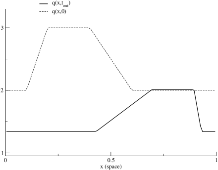
Figure 1. Burgers’s equation with linear source term. Initial condition (dash line) and the solution at time $t_{out}=0.2$ (full line) for $\beta=-2$ .

Figure 1, shows initial condition (75) and the solution of (57) at time $t_{out}=0.2$ for $\beta=-2\;.$

5. Burgers’s equation with a quadratic source term

Let us consider the partial differential equation

(78) $$\left.\begin{array}[]{c}\partial_{t}q(x,t)+\partial_{x}\biggl{(}\frac{q(x,t)^{2}}{2}\biggr{)}=\beta q(x,t)^{2}\;,\\ q(x,t)=h_{0}(x)\;.\end{array}\right\}$$

The equivalent ODE has the form

(81) $$\left.\begin{array}[]{c}\frac{d\hat{q}(t)}{dt}=\beta\hat{q}(t)^{2}\;,\\ \hat{q}(0)=h(0)\;,\end{array}\right\}$$

which is solvable and the exact solution is

(82) $$\hat{q}(t)=\mathcal{E}(t,h(0))=\frac{h(0)}{1-\beta th(0)}\;.$$

On the other hand, we note that the characteristic ODE

(85) $$\left.\begin{array}[]{c}\frac{d}{dt}x(t)=q(x,t)\;,\\ x(0)=y\;,\end{array}\right\}$$

for $q(x,t)$ satisfying (82) has the solution

(86) $$x=y-\frac{ln(1-\beta th_{0}(y))}{\beta}\;.$$

Therefore, the solution of (78) is given by

(87) $$q(x,t)=\frac{h_{0}(y)}{1-\beta th_{0}(y)}\;,$$

with $y$ satisfying (86).

Example 4.

Let us consider (78) in the interval $[0,1]\;,$ with initial condition

(88) $$h_{0}(x)=\sin(2\pi x)\;.$$

With this choice, $y$ is not explicitly obtained from (86). Therefore we use the bisection method. Figure 2, shows the initial condition (dash line ) and the solution at $t_{out}=0.15$ and for $\beta=-2\;.$

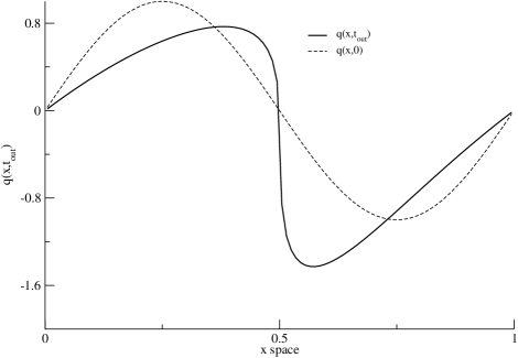
Figure 2. Burgers’s equation with quadratic source term. Initial condition (dash line) and the exact solution at time $t_{out}=0.15$ and for $\beta=-2\;.$

6. Burgers’s equation with a non-linear source term

Let us consider the partial differential equation

(91) $$\left.\begin{array}[]{c}\partial_{t}q(x,t)+\partial_{x}\biggl{(}\frac{q(x,t)^{2}}{2}\biggr{)}=e^{\beta q(x,t)}\;,\\ q(x,t)=h_{0}(x)\;.\end{array}\right\}$$

So, the equivalent ODE

(94) $$\left.\begin{array}[]{c}\frac{d\hat{q}(t)}{dt}=e^{\beta\hat{q}(t)}\;,\\ \hat{q}(0)=h(0)\;,\end{array}\right\}$$

has the exact solution

(95) $$\hat{q}(t)=\mathcal{E}(t,h(0))=-\frac{ln(e^{-\beta h(0)}-\beta t)}{\beta}\;.$$

On the other hand, the characteristic ODE

(98) $$\left.\begin{array}[]{c}\frac{d}{dt}x(t)=-\frac{ln(e^{-\beta h(0)}-\beta t)}{\beta}\;,\\ x(0)=y\;.\end{array}\right\}$$

with $\hat{q}(t)=q(x(t),t)$ satisfying (98) has the exact solution

(99) $$x=y+\frac{(e^{-\beta h_{0}(y)}-\beta t)ln(e^{-\beta h_{0}(y)}-\beta t)+\beta t+\beta h_{0}(y)e^{-\beta h_{0}(y)}}{\beta^{2}}\;.$$

Therefore, the solution to (91) is given by

(100) $$q(x,t)=-\frac{ln(e^{-\beta h_{0}(y)}-\beta t)}{\beta}\;,$$

with $y$ a solution of (99).

Example 5.

Let us consider (91) in the interval $[0,1]$, with the initial condition

(101) $$h_{0}(x)=2\biggl{(}\frac{1-w(x)}{2}\biggr{)}+\biggl{(}\frac{1+w(x)}{2}\biggr{)}\;.$$

with $w(x)=\displaystyle\frac{0.3-x}{\sqrt{(0.3-x)^{2}+\varepsilon}}\;.$ Figure 3 shows the initial condition for $\varepsilon=10^{-4}\;$ and the respective solution at time $t_{out}=0.26$ for $\beta=-1$.

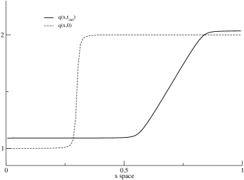
Figure 3. Bueger’s equation with exponential source term. Initial condition (dash line ) and solution at $t_{out}=0.26$ (full line). Parameters $\beta=-1\;$ and $\varepsilon=10^{-4}\;.$

7. Conclusions

In this work we have presented a procedure to obtain analytic solutions to the Burgers equation with a family of source terms aimed to provide a set of tests which is suitable for the assessment of numerical schemes. The family of source terms is that formed by functions containing primitive functions with respect to its arguments. By following the characteristic method, we have defined two ODE’s, which were called equivalent ODE and characteristic ODE. This family of source terms allows us the solvableness of these ODE’s and as a consequence the sought solution of the original PDE is found. In the solution of the characteristic ODE an algebraic equation, which depends on the initial condition, is obtained. The requirement of continuity for the initial condition allows us to find the root of this algebraic equation through the bisection method.

References

- [1] P. G. Estévez, C. Qu, and S. Zhang. Separation of variables of a generalized porous medium equation with nonlinear source. Journal of Mathematical Analysis and Applications, 275(1):44 – 59, 2002.
- [2] R.J. LeVeque. Numerical Methods for Conservation Laws. Lectures in Mathematics ETH Zürich, Department of Mathematics Research Institute of Mathematics. Springer, 1992.
- [3] G. Norgard and K. Mohseni. A regularization of the Burgers equation using a filtered convective velocity. Journal of Physics A: Mathematical and Theoretical, 41(344016):21 pp, 2008.
- [4] J.W. Thomas. Numerical Partial Differential Equations: Finite Difference Methods. Number v. 1 in Graduate Texts in Mathematics. Springer, 1995.
- [5] M. Wang, X. Li, and J. Zhang. The (G’/G)-expansion method and travelling wave solutions of nonlinear evolution equations in mathematical physics. Physics Letters A, 372(4):417 – 423, 2008.