Analyzing $b\to u$ transitions in semileptonic $\bar{B}_{s}\to K^{*+}(\to K\pi)\ell^{-}\bar{\nu}_{\ell}$ decays

Abstract

We study the semileptonic decay $\bar{B}_{s}\to K^{*+}\ell^{-}\bar{\nu}_{\ell}$, which is induced by $b\to u\ell^{-}\bar{\nu}_{\ell}$ transitions at the quark level. We take into account the standard model (SM) operator from $W$-boson exchange as well as possible extensions from physics beyond the SM. The secondary decay $K^{*+}\to K\pi$ can be used to study a number of angular observables, which are worked out in terms of short-distance Wilson coefficients and hadronic form factors. Our analysis allows for an independent extraction of the Cabibbo-Kobayashi-Maskawa matrix element $|V_{ub}|$ and for the determination of certain ratios of $\bar{B}_{s}\to K^{*}$ form factors. Moreover, a future precision measurement of the forward-backward asymmetry in the $\bar{B}_{s}\to K^{*+}\ell^{-}\bar{\nu}_{\ell}$ decay can be used to unambiguously verify the left-handed nature of the transition operator as predicted by the SM. We provide numerical estimates for the relevant angular observables and the resulting decay distributions on the basis of available form-factor information from lattice and sum-rule estimates. In addition, we pay particular attention to suitable combinations of angular observables in the decays $\bar{B}_{s}\to K^{*+}(\to K\pi)\ell^{-}\bar{\nu}_{\ell}$ and $\bar{B}\to K^{*0}(\to K\pi)\ell^{+}\ell^{-}$, and find that they provide complementary constraints on the relevant $b\to s$ short-distance coefficients. As a by-product, we perform a SM fit on the basis of selected experimental decay rates and hadronic input functions, which results in $|V_{ub}|=(4.07\pm 0.20)\cdot 10^{-3}$.

I Introduction

The value of $|V_{ub}|$ represents one of the least well-measured parameters in the Cabibbo-Kobayashi-Maskawa (CKM) matrix of the standard model (SM). Moreover, at present, its inclusive determination from $B\to X_{u}\ell\nu_{\ell}$ decays and the extraction from exclusive semileptonic or leptonic decay modes lead to somewhat different results (see e.g. the review in Kowalewski and Mannel (2014)). Independent phenomenological information on $b\to u$ transitions will clearly help to better understand the origin of these discrepancies and the underlying theoretical uncertainties. As the solution to this $|V_{ub}|$ puzzle might also be related to physics beyond the SM, one should also take into account possible new physics (NP) effects; see Buras et al. (2011); Dutta et al. (2013); Bernlochner et al. (2014) for recent work in that direction.

The proliferation of unknown parameters, which arises in a model-independent approach with generic dimension-6 operators in the effective Hamiltonian, can be handled with a sufficient number of independent experimental observables in $b\to u$ transitions. An example is $B\to\rho(\to\pi\pi)\ell\nu_{\ell}$ where the analysis of the secondary $\rho\to\pi\pi$ decay introduces a large number of angular observables with different sensitivities to the individual short-distance coefficients Bernlochner et al. (2014). This is similar to what has been extensively used in the analysis of rare exclusive $b\to s\ell^{+}\ell^{-}$ transitions Krüger et al. (2000); Krüger and Matias (2005); Egede et al. (2008); Altmannshofer et al. (2009); Bobeth et al. (2012); Böer et al. (2015). Because of the large hadronic width of the $\rho$ resonance and the question of the S- and P-wave composition of the experimentally measured dipion final state, a precision determination of $|V_{ub}|$ from this decay also requires a better theoretical understanding of the $B\to\pi\pi\ell\nu_{\ell}$ decay spectrum Faller et al. (2014); Kang et al. (2014).

In this article, we focus on the decay $\bar{B}_{s}\to K^{*+}(\to K\pi)\ell^{-}\bar{\nu}_{\ell}$, which provides similar insight into the short-distance couplings as the decay $B\to\rho(\to\pi\pi)\ell^{-}\bar{\nu}_{\ell}$. However, the width of the $K^{*}$-meson is sufficiently smaller than that of the $\rho$ resonance, $\Gamma_{K^{*}}\simeq\Gamma_{\rho}/4\simeq 50~{}\text{MeV}$. Moreover, from studies of the decay $\bar{B}\to\bar{K}^{*}J/\psi$ the S-wave background below the $K^{*}$ resonance in $B$ decays is constrained to small values, with the S-wave fraction $F_{s}\lesssim 7\%$ on-resonance Aaij et al. (2013a). The decay $\bar{B}_{s}\to K^{*+}(\to K\pi)\ell^{-}\bar{\nu}_{\ell}$ thus provides a promising alternative channel for a precise determination of $|V_{ub}|$ in the SM, as has already been advocated for in Meißner and Wang (2014). For the same reason, it can also be used to constrain NP contributions in $b\to u$ transitions, in particular, as we will show below, to exclude possible effects from right-handed currents.

Another benefit of the decay $\bar{B}_{s}\to K^{*+}\ell^{-}\bar{\nu}_{\ell}$ is the opportunity to combine it with the rare $\bar{B}\to\bar{K}^{*}\ell^{+}\ell^{-}$ decay. The secondary decay $K^{*}\to K\pi$ is identical in both decays, which leads to a one-to-one correspondence between angular observables. Hadronic form factors in both decays are related by the $SU(3)_{f}$ symmetry of the strong interaction, and therefore hadronic uncertainties in ratios of angular observables from the two decays are expected to be under control.

Furthermore, these ratios of angular observables are sensitive not only to $|V_{ub}|$, but also to bilinear combinations of the Wilson coefficients describing semileptonic $b\to u$ and radiative $b\to s$ transitions in the SM and beyond. In light of the present deviations between LHCb measurements and the respective SM predictions for a few angular observables in the $\bar{B}\to\bar{K}^{*}$ channel (see e.g. Aaij et al. (2013b); Matias et al. (2012), and also Jäger and Martin Camalich (2013)), we will show how this can be exploited to obtain complementary information on the $b\to s$ Wilson coefficients.

The outline of the article is as follows. In section II we introduce the effective Hamiltonian for semileptonic $b\to u\ell\bar{\nu}_{\ell}$ transitions, including NP operators, and define the angular observables for $\bar{B}_{s}\to K^{*}(\to K\pi)\ell\bar{\nu}_{\ell}$ transitions. In the following phenomenological section III we identify SM null tests among the angular observables, and derive expressions in a simplified scenario with only right-handed NP contributions. We also define optimized observables and highlight the synergies between the angular observables in $\bar{B}_{s}\to K^{*+}(\to K\pi)\ell\bar{\nu}_{\ell}$ and $\bar{B}\to K^{*}(\to K\pi)\ell^{+}\ell^{-}$. In the numerical section IV we first perform a fit of the Wilson coefficients for (V-A) and (V+A) currents to experimental data for $\bar{B}\to\pi^{+}\ell^{-}\bar{\nu}_{\ell}$, $B^{-}\to\tau^{-}\bar{\nu}_{\tau}$ and $\bar{B}\to X_{u}\ell^{-}\bar{\nu}_{\ell}$ decays. On the basis of this fit and theoretical estimates for the relevant form factors, we then provide numerical predictions for the angular observables and partially integrated branching ratios for $\bar{B}_{s}\to K^{*+}(\to K\pi)\ell\bar{\nu}_{\ell}$ decays, before we conclude in section V. The helicity basis for the $\bar{B}_{s}\to K^{*}$ form factors is defined in appendix A, where we also infer the form factor parameters from light-cone sum rule and lattice QCD results. The appendices B and C are dedicated to details on the determination of the hadronic amplitudes and the angular observables of $\bar{B}_{s}\to K^{*+}\ell^{-}\bar{\nu}_{\ell}$ decays within and beyond the SM, respectively.

II Definitions

II.1 Effective Hamiltonian for $b\to u\ell\bar{\nu}_{\ell}$

We parametrize possible new physics contributions to $b\to u\ell\bar{\nu}_{\ell}$ transitions in a model-independent fashion in terms of a low-energy effective Hamiltonian, which can be written in the form

$$\mathcal{H}^{\mathrm{eff}}_{b\to u}=-\frac{4G_{\rm F}V_{ub}^{\text{eff}}}{\sqrt{2}}\,\sum_{X}\mathcal{C}_{X}\,\mathcal{O}_{X}+\text{ h.c.}\,.$$ (1)

Here the most general set of dimension-6 operators $\{\mathcal{O}_{X}\}$ is given by

$$\mathcal{O}_{V,i} =\big{[}\bar{u}\gamma^{\mu}P_{i}b\big{]}\big{[}\bar{\ell}\gamma_{\mu}P_{L}\nu_{\ell}\big{]}\,,$$ (2)

$$\mathcal{O}_{S,i} =\big{[}\bar{u}P_{i}b\big{]}\big{[}\bar{\ell}P_{L}\nu_{\ell}\big{]}\,,$$

$$\mathcal{O}_{T} =\big{[}\bar{u}\sigma^{\mu\nu}b\big{]}\big{[}\bar{\ell}\sigma_{\mu\nu}P_{L}\nu_{\ell}\big{]}\,,$$

where $P_{i}\in\{P_{L},P_{R}\}$ are chiral projectors, and we have restricted ourselves to (massless) left-handed neutrinos and ignored the possibility of lepton-flavor violating couplings. (The generalization to more exotic scenarios with light right-handed invisible neutral fermions is straight-forward, see e.g. Dutta et al. (2013).) Since in the presence of NP the notion of $V_{ub}$ becomes ambiguous, we normalize the operators in eq. (1) to an effective parameter $V_{ub}^{\text{eff}}$, which can be taken, for instance, as the value of $V_{ub}$ that one obtains from a global CKM fit within the SM. If NP effects are small, one would then have $C_{V,L}\simeq 1$ (while in the SM $C_{V,L}\equiv 1$ and $V_{ub}\equiv V_{ub}^{\rm eff}$, with all other Wilson coefficients vanishing). Comparing with reference Buras et al. (2011), where the modifications of left- and right-handed quark currents has been parametrized in terms of $\varepsilon_{L,R}$ together with a new mixing-matrix $\tilde{V}$ for right-handed currents, our conventions are related via

$$\left(\frac{V_{ub}}{V_{ub}^{\text{eff}}}\right)\varepsilon_{L} =\mathcal{C}_{V,L}-1\,, \left(\frac{\tilde{V}_{ub}}{V_{ub}^{\text{eff}}}\right)\varepsilon_{R} =\mathcal{C}_{V,R}\,.$$ (3)

II.2 Angular distribution in $\bar{B}_{s}\to K^{*}\ell\bar{\nu}_{\ell}$

The four-fold differential decay rate for $\bar{B}_{s}\to K^{*+}\ell^{-}\bar{\nu}_{\ell}$ is defined in terms of the dilepton invariant mass $q^{2}$, the polar angles $\theta_{\ell}$ and $\theta_{K^{*}}$ in the $\ell\nu$ and $K^{*}$ rest frames, respectively, and the azimuthal angle $\phi$ between the primary and secondary decay planes,

$$\frac{8\pi}{3}\frac{{\rm d}^{4}\Gamma[\bar{B}_{s}\to K^{*}\ell^{+}\bar{\nu}_{\ell}]}{{\rm d}q^{2}\,{\rm d}\cos\theta_{\ell}\,{\rm d}\cos\theta_{K^{*}}\,{\rm d}\phi}=\hat{J}(q^{2},\theta_{\ell},\theta_{K^{*}},\phi)\,.$$ (4)

It can be expanded in a basis of trigonometric functions of the decay angles. We define

$$\hat{J}(q^{2},\theta_{\ell},\theta_{K^{*}},\phi) =\hat{J}_{1s}\sin^{2}\theta_{K^{*}}+\hat{J}_{1c}\cos^{2}\theta_{K^{*}}$$

$$+(\hat{J}_{2s}\sin^{2}\theta_{K^{*}}+\hat{J}_{2c}\cos^{2}\theta_{K^{*}})\cos 2\theta_{\ell}$$

$$+\hat{J}_{3}\sin^{2}\theta_{K^{*}}\sin^{2}\theta_{\ell}\cos 2\phi$$

$$+\hat{J}_{4}\sin 2\theta_{K^{*}}\sin 2\theta_{\ell}\cos\phi$$

$$+\hat{J}_{5}\sin 2\theta_{K^{*}}\sin\theta_{\ell}\cos\phi$$

$$+(\hat{J}_{6s}\sin^{2}\theta_{K^{*}}+\hat{J}_{6c}\cos^{2}\theta_{K^{*}})\cos\theta_{\ell}$$

$$+\hat{J}_{7}\sin 2\theta_{K^{*}}\sin\theta_{\ell}\sin\phi$$

$$+\hat{J}_{8}\sin 2\theta_{K^{*}}\sin 2\theta_{\ell}\sin\phi$$

$$+\hat{J}_{9}\sin^{2}\theta_{K^{*}}\sin^{2}\theta_{\ell}\sin 2\phi\,,$$ (5)

with angular observables $\hat{J}_{i(a)}\equiv\hat{J}_{i(a)}(q^{2})$ for $i=1,\dots,9$ and $a=s,c$. By construction, the functional dependence of the angular distribution eq. (5) on the angular observables is identical to the one for $B\to V(\to P_{1}P_{2})\ell^{+}\ell^{-}$ decays in Bobeth et al. (2012), to which we refer for further details.

Explicit expressions for the angular observables in terms of hadronic form factors and Wilson coefficients for $b\to u\ell\bar{\nu}_{\ell}$ in the general operator basis (1) are derived in the appendices.

III Phenomenology

For the remainder of this article we restrict our analysis to vector-like couplings; i.e., we assume $\mathcal{C}_{S,i}=\mathcal{C}_{T}=\mathcal{C}_{T5}=0$ for simplicity. This leaves us with only two operators for left- and right-handed $b\to u$ currents, which we refer to as SM+SM’. We emphasize that with future experimental data one can also test for scalar and tensor currents on the basis of the formulae provided in appendix C.

III.1 Null tests of the SM

The twelve angular observables $\hat{J}_{i}$ as introduced in eq. (5) are not independent. Within the SM, they can be expressed in terms of four real-valued quantities: $|N|^{2}$, and the three form factors $F_{\perp,\parallel,0}$. This fact can be used to define a series of eight null tests that hold within the SM:

$$4\hat{J}_{2c}\hat{J}_{3}+\hat{J}_{5}^{2}-4\hat{J}_{4}^{2} =0\,,$$ (6)

$$8\hat{J}_{1s}\hat{J}_{1c}-3\hat{J}_{5}^{2}-12\hat{J}_{4}^{2} =0\,,$$ (7)

$$\hat{J}_{1c}\hat{J}_{6s}-2\hat{J}_{4}\hat{J}_{5} =0\,,$$ (8)

$$16\hat{J}_{1s}^{2}-36\hat{J}_{3}^{2}-9\hat{J}_{6s}^{2} =0\,,$$ (9)

$$\hat{J}_{6c}=\hat{J}_{7}=\hat{J}_{8}=\hat{J}_{9} =0\,.$$ (10)

Deviations from these relations are immediate signs of physics beyond the SM. This is in contrast to exclusive $b\to s\ell^{+}\ell^{-}$ decays, where such relations are broken by nonfactorizing long-distance contributions.

III.2 Angular observables for SM+SM’

In the SM+SM’ scenario, we obtain a very simple structure of the angular observables, which can be expressed in terms of hadronic form factors (defined in the transversity basis, see appendix A), and three independent combinations of Wilson coefficients,

$$\sigma_{1}^{\pm} \equiv|\mathcal{C}_{V,L}\pm\mathcal{C}_{V,R}|^{2}\,,$$ (11)

$$-2\sigma_{2} \equiv(\mathcal{C}_{V,L}-\mathcal{C}_{V,R})(\mathcal{C}_{V,L}+\mathcal{C}_{V,R})^{*}\,,$$

which depend on the absolute values $|C_{V,L}|$ and $|C_{V,R}|$ and the relative phase of the two Wilson coefficients (the absolute phase is irrelevant in the angular observables). Notice that $\sigma_{1}^{\pm}$ is even under parity transformations ($L\leftrightarrow R$), while $\sigma_{2}$ is odd. Neglecting the charged-lepton mass (which is valid as long as $m_{\ell}/\sqrt{q^{2}}\ll 1$), we find

$$\hat{J}_{1s} =3\,\hat{J}_{2s}=9\,|N|^{2}\,M_{B_{s}}^{2}\Big{[}\sigma_{1}^{+}\,|F_{\perp}|^{2}+\sigma_{1}^{-}\,|F_{\parallel}|^{2}\Big{]}\,,$$ (12)

$$\hat{J}_{1c} =-\hat{J}_{2c}=12\,|N|^{2}\,\frac{M_{B_{s}}^{4}}{q^{2}}\,\sigma_{1}^{-}\,|F_{0}|^{2}\,,$$ (13)

$$\hat{J}_{3} =6\,|N|^{2}\,M_{B_{s}}^{2}\Big{[}\sigma_{1}^{+}\,|F_{\perp}|^{2}-\sigma_{1}^{-}\,|F_{\parallel}|^{2}\Big{]}\,,$$ (14)

$$\hat{J}_{4} =6\sqrt{2}\,|N|^{2}\,\frac{M_{B_{s}}^{3}}{\sqrt{q^{2}}}\,\sigma_{1}^{-}\,F_{\parallel}\,F_{0}\,,$$ (15)

and

$$\hat{J}_{5} =24\,\sqrt{2}\,|N|^{2}\,\frac{M_{B_{s}}^{3}}{\sqrt{q^{2}}}\,{\rm Re}\left\{{\sigma_{2}}\right\}\,F_{\perp}\,F_{0}\,,$$ (16)

$$\hat{J}_{6s} =48\,|N|^{2}\,M_{B_{s}}^{2}\,{\rm Re}\left\{{\sigma_{2}}\right\}\,F_{\perp}\,F_{\parallel}\,,$$ (17)

$$\hat{J}_{8} =12\,\sqrt{2}\,|N|^{2}\,\frac{M_{B_{s}}^{3}}{\sqrt{q^{2}}}\,{\rm Im}\left\{{\sigma_{2}}\right\}\,F_{\perp}\,F_{0}\,,$$ (18)

$$\hat{J}_{9} =24\,|N|^{2}\,M_{B_{s}}^{2}\,{\rm Im}\left\{{\sigma_{2}}\right\}\,F_{\perp}\,F_{\parallel}\,,$$ (19)

together with $\hat{J}_{6c}=\hat{J}_{7}=0$ (all relations valid in the SM+SM’ scenario). Here, we introduce a normalization factor,

$$|N|^{2}\equiv\frac{G^{2}_{\text{F}}|V_{ub}^{\rm eff}|^{2}q^{2}\sqrt{\lambda}}{3\cdot 2^{10}\pi^{3}M_{B_{s}}^{3}}\,,$$ (20)

and $\lambda\equiv\lambda(M_{B}^{2},M_{K^{*}}^{2},q^{2})$ denotes the usual kinematic Källén function. The normalization $|N|^{2}$ is chosen such that

$$\frac{{\rm d}\Gamma}{{\rm d}q^{2}} =\sum_{\lambda=0,\perp,\parallel}|A^{L}_{\lambda}|^{2}$$ (21)

$$=|N|^{2}M_{B_{s}}^{2}\left[\sigma_{1}^{+}|F_{\perp}|+\sigma_{1}^{-}\left(|F_{\parallel}|^{2}+\frac{M_{B_{s}}^{2}}{q^{2}}|F_{0}|^{2}\right)\right]\,,$$

where the transversity amplitudes $A_{\lambda}^{L}$ are defined in appendix B.

Beside the decay rate, one can also define the leptonic forward-backward asymmetry $A_{\rm FB}$ via the weighted integral

$$A_{\rm FB}\equiv\frac{1}{{\rm d}\Gamma/{\rm d}q^{2}}\int_{-1}^{+1}{\rm d}\cos\theta_{\ell}\,\operatorname{sgn}(\cos\theta_{\ell})\frac{{\rm d}^{2}\Gamma}{{\rm d}q^{2}\,{\rm d}\cos\theta_{\ell}}\,.$$ (22)

In the SM+SM’ scenario, one finds that $A_{\rm FB}$ takes the rather simple form

$$A_{\rm FB}=\frac{2{\rm Re}\left\{{\sigma_{2}}\right\}F_{\perp}F_{\parallel}}{\sigma_{1}^{+}|F_{\perp}|^{2}+\sigma_{1}^{-}\left(|F_{\parallel}|^{2}+\frac{M_{B_{s}}^{2}}{q^{2}}|F_{0}|^{2}\right)}\,.$$ (23)

Note, that the bilinear $\sigma_{2}$ is unconstrained by present experimental measurements of semileptonic $b\to u$ transitions. Therefore a measurement of $A_{\rm FB}$ would provide complementary information on the Wilson coefficients. In particular, the sign of the forward-backward asymmetry resolves the present ambiguity between $\mathcal{C}_{V,L}$ versus $\mathcal{C}_{V,R}$, see section IV.

Similarly, the fraction of longitudinal $K^{*}$ mesons is defined as

$$F_{L}\equiv\frac{1}{{\rm d}\Gamma/{\rm d}q^{2}}\int_{-1}^{+1}{\rm d}\!\cos\theta_{K^{*}}\,\omega_{F_{L}}(\cos\theta_{K^{*}})\frac{{\rm d}^{2}\Gamma}{{\rm d}q^{2}\,{\rm d}\!\cos\theta_{K^{*}}}\,,$$ (24)

where $\omega_{F_{L}}(z)=(5z^{2}-1)/2$. In the SM+SM’ scenario this yields

$$F_{L}=\frac{\sigma_{1}^{-}|F_{0}|^{2}}{\sigma_{1}^{+}|F_{\perp}|^{2}+\sigma_{1}^{-}\left(|F_{\parallel}|^{2}+\frac{M_{B_{s}}^{2}}{q^{2}}|F_{0}|^{2}\right)}\,.$$ (25)

III.3 Optimized observables in SM+SM’

It is now possible to construct particular combinations of angular observables where the hadronic form-factor dependencies cancel (at least partially), and, as a consequence, these observables are sensitive to the short-distance Wilson coefficients, only; or vice-versa.

We begin with observables where the form-factor dependencies cancel. These can be defined in complete analogy to what has been discussed in Bobeth et al. (2012),

$$\hat{H}_{T}^{(1)} =\frac{\sqrt{2}\hat{J}_{4}}{\sqrt{-\hat{J}_{2c}(2\hat{J}_{2s}-\hat{J}_{3})}}\,,$$ (26)

$$\hat{H}_{T}^{(2)} =\frac{\hat{J}_{5}}{\sqrt{-2\hat{J}_{2c}(2\hat{J}_{2s}+\hat{J}_{3})}}\,,$$ (27)

$$\hat{H}_{T}^{(3)} =\frac{\hat{J}_{6s}}{2\sqrt{(2\hat{J}_{2c})^{2}-(\hat{J}_{3})^{2}}}\,,$$ (28)

$$\hat{H}_{T}^{(4)} =\frac{2\hat{J}_{8}}{\sqrt{-2\hat{J}_{2c}(2\hat{J}_{2s}+\hat{J}_{3})}}\,,$$ (29)

$$\hat{H}_{T}^{(5)} =\frac{-\hat{J}_{9}}{\sqrt{(2\hat{J}_{2c})^{2}-(\hat{J}_{3})^{2}}}\,.$$ (30)

Within the SM+SM’ scenario, the form factors dependencies cancel exactly at every point in the $q^{2}$ spectrum. However, for integrated angular observables one has to take into account the different kinematical prefactors, and a residual form-factor dependence will remain. In the SM+SM’ scenario these optimized observables read

$$\hat{H}_{T}^{(1)} =1\,,$$ (31)

$$\hat{H}_{T}^{(2)} =\hat{H}_{T}^{(3)}=2\,\frac{{\rm Re}\left\{{\sigma_{2}}\right\}}{\sqrt{\sigma_{1}^{+}\sigma_{1}^{-}}}\,,$$

$$\hat{H}_{T}^{(4)} =\hat{H}_{T}^{(5)}=2\,\frac{{\rm Im}\left\{{\sigma_{2}}\right\}}{\sqrt{\sigma_{1}^{+}\sigma_{1}^{-}}}\,.$$

We continue with the construction of observables that are only sensitive to form-factor ratios. Just as in $\bar{B}\to\bar{K}^{*}\ell^{+}\ell^{-}$, we find that the SM+SM’ scenario solely allows us to extract one form factor ratio, namely $F_{0}/F_{\parallel}$, in five different ratios of angular observables,

$$\frac{M_{B_{s}}}{\sqrt{q^{2}}}\frac{F_{0}(q^{2})}{F_{\parallel}(q^{2})}=\frac{\sqrt{2}\hat{J}_{5}}{\hat{J}_{6s}}=\frac{-\hat{J}_{2c}}{\sqrt{2}J_{4}}\\ =\frac{\hat{J}_{4}}{2\hat{J}_{2s}-\hat{J}_{3}}=\sqrt{\frac{-\hat{J}_{2c}}{2\hat{J}_{2s}-\hat{J}_{3}}}=\frac{\sqrt{2}\hat{J}_{8}}{-\hat{J}_{9}}\,.$$ (32)

Inconsistencies among these relations would indicate NP beyond the SM+SM’ scenario.

III.4 Synergies with $\bar{B}\to\bar{K}^{*}\ell^{+}\ell^{-}$

The decay $\bar{B}\to\bar{K}^{*}(\to\bar{K}\pi)\ell^{+}\ell^{-}$ is induced by the flavor-changing neutral current (FCNC) transition $b\to s\ell^{+}\ell^{-}$. At low hadronic recoil, $q^{2}\gtrsim 15~{}\text{GeV}^{2}$, it is again dominated by four-fermion operators which can be extended to a SM+SM’ scenario. The structure of angular observables $J_{n}(q^{2})$ in those decays is similar as for $\bar{B}_{s}\to\bar{K}^{*+}\ell\bar{\nu}_{\ell}$. The analogous combinations of Wilson coefficients which enter the $J_{n}(q^{2})$ now read $\rho_{1}^{\pm}$ and $\rho_{2}$. (For the explicit definition and a detailed phenomenological discussion, we refer to Bobeth et al. (2012).)

With this we can define a number of useful ratios of angular observables $J_{n}(q^{2})$ in $\bar{B}\to\bar{K}^{*}\ell^{+}\ell^{-}$ and $\hat{J}_{n}(q^{2})$ in $\bar{B}_{s}\to\bar{K}^{*+}\ell\bar{\nu}_{\ell}$,

$$R_{n}(q^{2})\equiv\frac{J_{n}(q^{2})}{\hat{J}_{n}(q^{2})}\,,$$ (33)

for $n=1c,2c,4,5,6s,8,9$, as well as

$$R_{1\pm}(q^{2}) \equiv\frac{2J_{1s}(q^{2})\pm 3J_{3}(q^{2})}{2\hat{J}_{1s}(q^{2})\pm 3\hat{J}_{3}(q^{2})}\,,$$ (34)

$$R_{2\pm}(q^{2}) \equiv\frac{2J_{2s}(q^{2})\pm J_{3}(q^{2})}{2\hat{J}_{2s}(q^{2})\pm\hat{J}_{3}(q^{2})}\,.$$

Within these ratios, the dependence on the hadronic form factors can be expected to cancel up to corrections from the violation of the $SU(3)_{f}$ symmetry of strong interactions, and from nonfactorizing hadronic matrix elements in exclusive $b\to s\ell^{+}\ell^{-}$ transitions. In the limit where these corrections are neglected, we find

$$R_{n}\simeq\frac{\alpha_{e}^{2}}{8\pi^{2}}\,\frac{|V_{tb}V^{*}_{ts}|^{2}}{|V_{ub}|^{2}}\begin{cases}\displaystyle\frac{\rho_{1}^{+}}{\sigma_{1}^{+}}&\text{for }n=1+,2+\\ \displaystyle\frac{\rho_{1}^{-}}{\sigma_{1}^{-}}&\text{for }n=1-,1c,2-,2c\\ \displaystyle\frac{{\rm Re}\left\{{\rho_{2}}\right\}}{{\rm Re}\left\{{\sigma_{2}}\right\}}&\text{for }n=4,5,6s\\ \displaystyle\frac{{\rm Im}\left\{{\rho_{2}}\right\}}{{\rm Im}\left\{{\sigma_{2}}\right\}}&\text{for }n=8,9\\ \end{cases}\,.$$ (35)

Of particular interest are ratios that are proportional to the combination $\rho_{2}\propto{\rm Re}\left\{{\mathcal{C}_{79}(q^{2})\,\mathcal{C}^{*}_{10}}\right\}$, where in the SM $\mathcal{C}_{79}(q^{2})$ is a linear combination of the Wilson coefficients $\mathcal{C}^{\rm eff}_{7}$ and $\mathcal{C}^{\rm eff}_{9}(q^{2})$ in $b\to s$ transitions (see Bobeth et al. (2012) for the explicit definitions). Optimized observables in $\bar{B}\to\bar{K}^{*}\ell^{+}\ell^{-}$ only allow to access the ratio $|\mathcal{C}^{\rm eff}_{9}/\mathcal{C}_{10}|$, whereas the ratios $R_{n}$ are sensitive to $\mathcal{C}^{\rm eff}_{9}\cdot\mathcal{C}_{10}$. Measuring the corresponding ratios $J_{n}/\hat{J}_{n}$ thus allows to directly access the $q^{2}$ dependence of $\mathcal{C}^{\rm eff}_{9}$ and to test the theoretical predictions which are based on an operator product expansion in the heavy $b$-quark limit.

IV Numerical Results

Decay	$q^{2}$ [GeV2]	Measurement	Reference
$B^{-}\to\tau^{-}\bar{\nu}_{\tau}$	–	$(1.70\pm 0.80\pm 0.20)\cdot 10^{-4}$	Aubert et al. (2010)
	–	$(1.25\pm 0.28\pm 0.27)\cdot 10^{-4}$	Kronenbitter et al. (2015)
	–	$(1.83^{+0.53}_{-0.59}\pm 0.24)\cdot 10^{-4}$	Lees et al. (2013)
	–	$(0.72^{+0.27}_{-0.25}\pm 0.11)\cdot 10^{-4}$	Adachi et al. (2013)
$\bar{B}^{0}\to\pi^{+}\mu^{-}\bar{\nu}_{\tau}$	$[0,2]$	$(1.280\pm 0.196)\cdot 10^{-5}$	del Amo Sanchez et al. (2011)
	$[2,4]$	$(1.192\pm 0.135)\cdot 10^{-5}$
	$[4,6]$	$(1.446\pm 0.108)\cdot 10^{-5}$
	$[6,8]$	$(1.437\pm 0.105)\cdot 10^{-5}$
	$[8,10]$	$(1.525\pm 0.106)\cdot 10^{-5}$
	$[10,12]$	$(1.490\pm 0.111)\cdot 10^{-5}$
	$[0,2]$	$(1.173\pm 0.219)\cdot 10^{-5}$	Ha et al. (2011)
	$[2,4]$	$(1.526\pm 0.103)\cdot 10^{-5}$
	$[4,6]$	$(1.213\pm 0.105)\cdot 10^{-5}$
	$[6,8]$	$(1.465\pm 0.102)\cdot 10^{-5}$
	$[8,10]$	$(1.473\pm 0.108)\cdot 10^{-5}$
	$[10,12]$	$(1.404\pm 0.124)\cdot 10^{-5}$
	$[0,2]$	$(1.225\pm 0.182)\cdot 10^{-5}$	Lees et al. (2012)
	$[2,4]$	$(1.277\pm 0.128)\cdot 10^{-5}$
	$[4,6]$	$(1.274\pm 0.109)\cdot 10^{-5}$
	$[6,8]$	$(1.498\pm 0.103)\cdot 10^{-5}$
	$[8,10]$	$(1.405\pm 0.115)\cdot 10^{-5}$
	$[10,12]$	$(1.617\pm 0.104)\cdot 10^{-5}$
	$[0,2]$	$(1.95\pm 0.32)\cdot 10^{-5}$	Sibidanov et al. (2013)
	$[2,4]$	$(1.06\pm 0.27)\cdot 10^{-5}$
	$[4,6]$	$(1.51\pm 0.28)\cdot 10^{-5}$
	$[6,8]$	$(0.97\pm 0.23)\cdot 10^{-5}$
	$[8,10]$	$(0.78\pm 0.22)\cdot 10^{-5}$
	$[10,12]$	$(1.59\pm 0.28)\cdot 10^{-5}$

Table 1: Summary of the experimental likelihoods for branching fractions of the exclusive $b\to u$ transitions. We assume no correlation among the $B^{-}\to\tau^{-}\bar{\nu}_{\tau}$ data, and use the correlation matrices as given in (del Amo Sanchez et al., 2011, tables XI and XII), (Ha et al., 2011, table III and IV), (Lees et al., 2012, tables XXIX and XXXII) and (Sibidanov et al., 2013, table XVII) for the respective data on $\bar{B}^{0}\to\pi^{+}\mu^{-}\bar{\nu}_{\mu}$ decays.

In this section we derive numerical results for the angular observables $\hat{J}_{n}$ as introduced in section II.2. Our analysis is carried out within a Bayesian framework, for which we use and extend EOS van Dyk et al. for all numerical evaluations. As prerequisites to our numerical study of the angular observables, information on the $\bar{B}_{s}\to K^{*}$ form factors, and constraints on the $b\to u$ Wilson coefficients are needed. These will be expressed through a-posteriori probability density functions (PDFs) labelled $P(\vec{\theta}_{\text{FF}}|\text{theory})$ and $P(\vec{\theta}_{\Delta B}|\text{exp. data})$, respectively. We refer to appendix A for the precise definition of $P(\vec{\theta}_{\text{FF}}|\text{theory})$.

IV.1 Determination of $C_{V,L}$ and $C_{V,R}$

For the following numerical analysis we consider experimental data on the branching ratios for leptonic $B^{-}\to\tau^{-}\bar{\nu}_{\tau}$ and semileptonic $\bar{B^{0}}\to\pi^{+}\mu^{-}\bar{\nu}_{\mu}$ decays as summarized in table 1, together with the averaged value for $|V_{ub}|$ from the inclusive determination,

$$|V_{ub}^{\text{incl.}}| =(4.41\pm 0.21)\cdot 10^{-3}\quad\text{\cite[cite]{\@@bibref{Authors Phrase1YearPhrase2}{Kowalewski:2014PDG}{\@@citephrase{(}}{\@@citephrase{)}}}}\,.$$ (36)

Within the SM+SM’ scenario, the additional right-handed operator contributes differently to the individual decay rates, corresponding to (see e.g. Buras et al. (2011))

$$|V_{ub}^{B\to\tau\nu}|^{2} \to|V_{ub}^{\text{eff}}|^{2}\left|\mathcal{C}_{V,L}-\mathcal{C}_{V,R}\right|^{2}\,,$$ (37)

$$|V_{ub}^{B\to\pi\ell\nu}|^{2} \to|V_{ub}^{\text{eff}}|^{2}\left|\mathcal{C}_{V,L}+\mathcal{C}_{V,R}\right|^{2}\,,$$

$$|V_{ub}^{\text{incl.}}|^{2} \to|V_{ub}^{\text{eff}}|^{2}\left(|\mathcal{C}_{V,L}|^{2}+|\mathcal{C}_{V,R}|^{2}\right)\,.$$

In order to illustrate the NP reach of our analysis, we fix the auxiliary parameter $V_{ub}^{\text{eff}}$ to a value that lies between the exclusive and inclusive determinations of $|V_{ub}|$ within the SM,

$$|V_{ub}^{\text{eff}}|\equiv 3.99\cdot 10^{-3}\,.$$

With this we can constrain the absolute values and the relative phases of the Wilson coefficients $\mathcal{C}_{V,L}$ and $\mathcal{C}_{V,R}$, where the SM-like solution would correspond to $|\mathcal{C}_{V,L}|\sim 1$ and $\mathcal{C}_{V,R}\sim 0$.

We construct a likelihood $P(\text{data}|\vec{\theta}_{\Delta B},M)$ from (multi)normal distributions as indicated in table 1 and eq. (36). Note that we assume that the results for the $B^{-}\to\tau^{-}\bar{\nu}_{\tau}$ branching ratios Aubert et al. (2010) and Lees et al. (2013) are uncorrelated, since the underlying sets of events use different tagging methods for the selection process. The same assumption applies to the results of Adachi et al. (2013) and Hara et al. (2010). At this time, we only use theoretical input from light-cone sum rules for the $B\to\pi$ transition form factors, and therefore restrict ourselves to the kinematic range $q^{2}\leq 12~{}\text{GeV}^{2}$. For a consistent inclusion of lattice results on the $B\to\pi$ form factor in the high-$q^{2}$ region (see e.g. Dalgic et al. (2006); Bailey et al. (2009); Al-Haydari et al. (2010), but also note added below), we presently do not have access to the necessary correlation information required for our statistical procedure.

Within our analysis, we address the theoretical uncertainties using nuisance parameters for the hadronic matrix elements. These are the $B$-meson decay constant $f_{B^{-}}$, and the parameters of the the $B\to\pi$ vector form factor $f^{B\pi}_{+}(q^{2})$: its normalization $f^{B\pi}_{+}(0)$, as well as two shape parameters $b^{B\pi}_{1,2}$; see Imsong et al. (2014) for their definition. For the $B$-meson decay constant we use a Gaussian prior with central value and minimal $68\%$ probability interval $f_{B^{-}}=(210\pm 11)~{}\text{MeV}$, as obtained from a recent 2-point QCD sum rule at NNLO accuracy Gelhausen et al. (2013). As prior for the form factor parameters we use the a-posteriori distribution obtained from a recent Bayesian analysis of the LCSR prediction at NLO accuracy Imsong et al. (2014).

In order to assess the physical implications of possible deviations from the SM expectations, we compare the fit results for three different scenarios. In all cases we assume $C_{V,L}$ to be real-valued (i.e. a possible NP phase in the left-handed $b\to u$ transition should be associated to $V_{ub}^{\rm eff}$). As already mentioned, the fit to the considered data is only sensitive to the relative phase between the Wilson coefficients $C_{V,L}$ and $C_{V,R}$, and consequently we will always encounter an irreducible degeneracy related to $C_{V,L/R}\to-C_{V,L/R}$.

1. First, we consider the scenario “left” that features only the left-handed current. In this case the number of parameters is five, $\vec{\theta}^{\text{left}}_{\Delta B}=\left(\mathcal{C}_{V,L},f^{B\pi}_{+}(0),b^{B\pi}_{1},b^{B\pi}_{2},f_{B^{-}}\right)$.

2. Next, we consider the scenario “real”, in which $\mathcal{C}_{V,R}$ is present and real-valued. The set of $\Delta B$ parameters then reads $\vec{\theta}^{\text{real}}_{\Delta B}=\left(\mathcal{C}_{V,L},\operatorname{Re}\mathcal{C}_{V,R},f^{B\pi}_{+}(0),b^{B\pi}_{1},b^{B\pi}_{2},f_{B^{-}}\right)$.

3. Last but not least, we also consider the scenario “comp”, which includes a complex-valued $\mathcal{C}_{V,R}$, with the full seven parameters, $\vec{\theta}^{\text{comp}}_{\Delta B}=\big{(}\mathcal{C}_{V,L},\operatorname{Re}\mathcal{C}_{V,R},\operatorname{Im}\mathcal{C}_{V,R},f^{B\pi}_{+}(0),b^{B\pi}_{1},b^{B\pi}_{2},f_{B^{-}}\big{)}$.

For all scenarios ($M=\text{left},\text{real},\text{comp}$), we obtain the a-posteriori PDF as usual via Bayes’ theorem,

$$P(\vec{\theta}_{\Delta B}|\text{data},M)=\frac{P(\text{data}|\vec{\theta}_{\Delta B},M)P_{0}(\vec{\theta}_{\Delta B},M)}{P(\text{data},M)}\,,$$ (38)

where

$$P(\text{data},M)\equiv\int{\rm d}\vec{\theta}_{\Delta B}\,P(\text{data}|\vec{\theta}_{\Delta B},M)P_{0}(\vec{\theta}_{\Delta B},M)$$ (39)

is the evidence for the scenario $M$. The likelihood $P(\text{data}|\vec{\theta}_{\Delta B},M)$ has already been introduced earlier. In all three scenarios, we use for the priors of the Wilson coefficients uncorrelated, uniform distributions with the support $-2\leq\mathcal{C}_{i}\leq+2$. For model comparisons, we normalize the model priors for the various fits scenarios. The corresponding relations read

$$P_{0}(\text{comp}):P_{0}(\text{real}):P_{0}(\text{left})=1:4:16$$ (40)

	Significance [$\sigma$]
Quantity	“left”	“real”	“comp”	d.o.f.	Reference
$f_{+}(\dagger)$	$3.11$	$2.36$	$2.36$	3	Imsong et al. (2014)
$B^{-}\to\tau^{-}\bar{\nu}_{\tau}$	$+0.57$	$+0.39$	$+0.39$	1	Aubert et al. (2010)
	$+0.64$	$+0.34$	$+0.34$	1	Kronenbitter et al. (2015)
	$+0.99$	$+0.75$	$+0.75$	1	Lees et al. (2013)
	$-1.84$	$-2.35$	$-2.35$	1	Adachi et al. (2013)
$\bar{B}^{0}\to\pi^{+}\mu^{-}\bar{\nu}_{\tau}$	$0.85$	$1.08$	$1.08$	6	del Amo Sanchez et al. (2011)
	$0.87$	$0.98$	$0.98$	6	Ha et al. (2011)
	$1.70$	$1.97$	$1.97$	6	Lees et al. (2012)
	$2.53$	$2.46$	$2.46$	6	Sibidanov et al. (2013)
$\bar{B}\to X_{u}\ell^{-}\bar{\nu}_{\ell}$	$+1.67$	$+1.45$	$+1.45$	1	Kowalewski and Mannel (2014)

Table 2: Significances of the measurements at the best-fit point closest to the SM point for all three fit scenarios. Notice that the pull for the LCSR calculation of the $B\to\pi$ vector form factor $f_{+}$, marked by a $\dagger$, does not enter the goodness-of-fit calculation.

IV.1.1 Scenario “Left”

Our findings for the scenario “left” can be summarized as follows. We find two degenerate best-fit points corresponding to $|\mathcal{C}_{V,L}|\simeq 1$. The best-fit point (with positive $C_{V,L}$) reads

$$\vec{\theta}_{\Delta B}^{\text{left,$*$}}=\\ (1.016,0.232,-3.163,+0.425,0.206)\,.$$ (41)

We find at this point $\chi^{2}_{\text{left}}=18.54$, for $28$ degrees of freedom (from $29$ measurements reduced by $1$ fit parameter). As a consequence, this represents an excellent fit with a p-value of $91\%$. The significances of the individual experimental inputs are collected in table 2. The one-dimensional marginalized posterior is approximately Gaussian, and yields

$$|\mathcal{C}_{V,L}|=1.02\pm 0.05\quad\text{at $68\%$ probability}\,.$$ (42)

Equivalently, this result can be expressed as $|V_{ub}|=(4.07\pm 0.20)\cdot 10^{-3}$ at $68\%$ probability.

IV.1.2 Scenario “Real”

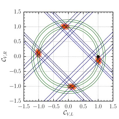
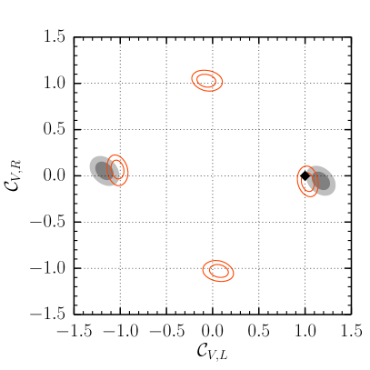
Figure 1: (left) Contours of the $68\%$ (dark orange area) and $95\%$ (orange area) probability regions for the Wilson coefficients $\mathcal{C}_{V,L}$ and $\mathcal{C}_{V,R}$ as obtained from our fit. See the text for details. Overlaid are the $68\%$ and $95\%$ contour lines for $\bar{B}^{0}\to\pi^{+}\ell^{-}\bar{\nu}_{\ell}$ (blue solid lines, negative slope), $B^{-}\to\ell^{-}\bar{\nu}_{\ell}$ (blue solid lines, positive slope) and inclusive $\bar{B}\to X_{u}\ell^{-}\bar{\nu}_{\ell}$ (green solid rings). The black diamond marks the SM point. (right) Contours of the $68\%$ and $95\%$ probability regions for the Wilson coefficients (solid orange lines) overlaying the $68\%$ (dark gray area) and $95\%$ (light gray area) probability regions as obtained from a hypothetical measurement of $A_{\rm FB}=A_{\rm FB}^{\text{SM}}\pm 10\%$.

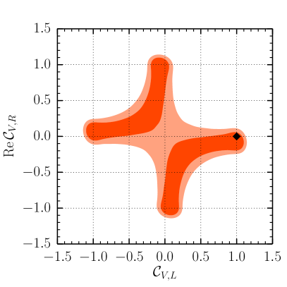
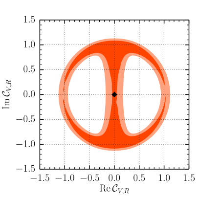
Figure 2: Contours of the $68\%$ (dark orange area) and $95\%$ (orange area) probability regions for the Wilson coefficients $\mathcal{C}_{V,L}$ and $\mathcal{C}_{V,R}$ as obtained from our fit in scenario “comp”. See the text for details. The black diamond marks the SM point.

For the scenario “real”, we find a four-fold ambiguity in the data; see figure 1 for an illustration. All local modes are degenerate. We calculate the goodness of fit in the local mode closest to the SM,

$$\vec{\theta}_{\Delta B}^{\text{real,$*$}}=\\ (1.025,-0.079,0.251,-2.884,+0.196,0.200)\,,$$ (43)

and obtain $\chi^{2}_{\text{real}}=20.47$. This fit’s p-value of $81\%$ is very good. However, note that the $\chi^{2}$ value has increased in comparison to the previous scenario. This result warrants a comment. The additional degree of freedom in form of $\mathcal{C}_{V,R}$ allows the fit to move the form factor parameters $f^{+}_{B\pi}$, $b_{1}$ and $b_{2}$ closer to the central values of the prior. This shift occurs at the expense of increasing the significances of the experimental data, while simultaneously reducing the significance of the nuisance parameters. For completeness, we also list these significances for all scenarios in table 2. The one-dimensional marginalized posterior distributions for this scenario are approximately Gaussian and symmetric under exchange $\mathcal{C}_{V,L}\leftrightarrow\operatorname{Re}\mathcal{C}_{V,R}$. We find (at 68% propabality)

$$|\mathcal{C}_{V,L}|=1.02\pm 0.05\quad \text{and}\quad|\operatorname{Re}C_{V,R}|\leq 0.10\,,$$ (44)

or (45)

$$|\operatorname{Re}\,\mathcal{C}_{V,R}|=1.02\pm 0.05\quad \text{and}\quad|\mathcal{C}_{V,L}|\leq 0.10\,.$$ (46)

IV.1.3 Scenario “Comp”

We repeat the fit in scenario “comp”. As a consequence of the additional degree of freedom, the four solutions from the previous scenario now become connected. This is illustrated in figure 2. We calculate the goodness of fit in the local mode closest to the SM, which now reads:

$$\vec{\theta}_{\Delta B}^{\text{comp,$*$}}=\\ (1.025,-0.080,0.000,0.251,-2.885,+0.196,0.200)\,.$$ (47)

The individual significances are listed in table 2, and amount to a total $\chi^{2}=20.48$. For the increase of $\chi^{2}$ with respect to the “left” scenario, see our earlier comment. With $26$ degrees of freedom the p-value is $77\%$, which is still very good. It is not sensible to provide the $68\%$ probability interval of the one-dimensional marginalized posterior, since the solutions are strongly connected. We show the contours of the probability regions at $68\%$ and $95\%$ probability in figure 2.

IV.1.4 Comparison

We proceed with a comparison of the various fit scenarios by means of the posterior odds. The latter can be calculated as

$$\frac{P(M_{1}|\text{data})}{P(M_{2}|\text{data})}=\frac{P(\text{data}|M_{1})}{P(\text{data}|M_{2})}\frac{P_{0}(M_{1})}{P_{0}(M_{2})}$$ (48)

We find

$$\frac{P(\text{``left''}|\text{data})}{P(\text{``real''}|\text{data})}=27.8\,:\,1\,,$$ (49)

and

$$\frac{P(\text{``real''}|\text{data})}{P(\text{``comp''}|\text{data})}=3.62\,:\,1\,.$$ (50)

Using Jeffrey’s scale for the interpretation of the posterior odds Jeffreys (1998), we find that the data favour the interpretation with purely left-handed $b\to u$ currents over the other scenarios very strongly. Moreover, the scenario “real” is substantially favored over the scenario “comp”.

This means that – despite the observed tensions between the different SM determinations of $|V_{ub}|$ – a NP scenario with right-handed currents does not lead to a more efficient description of the experimental data. We emphasize again that the statistical treatment of the theoretical uncertainties on the hadronic input parameters, which are still relatively large at present, has been crucial for this argument. On the other hand, the experimental data on the inclusive and exclusive decay rates alone also cannot exclude large right-handed currents.

IV.2 Predictions for Angular Observables $\hat{J}_{n}$

We can now proceed to produce predictive distributions for the angular observables $\hat{J}_{n}$ in $\bar{B}_{s}\to K^{*+}(\to K\pi)\ell\bar{\nu}_{\ell}$, for which we have two main applications in mind.

IV.2.1 SM Scenario

First, we assume the SM case; i.e., we go back to $V_{ub}^{\rm eff}\to V_{ub}$ with $\mathcal{C}_{V,L}\equiv 1$ and $\mathcal{C}_{i}\equiv 0$. In this case, only the a-posteriori PDF on the $\bar{B}_{s}\to K^{*}$ form factors is needed. We obtain the joint posterior-predictive distribution for the angular observables by means of

$$P(\vec{\hat{J}})=\int{\rm d}\vec{\theta}_{\text{FF}}\,P(\vec{\theta}_{\text{FF}}|\text{theory})\,\delta(\vec{\hat{J}}-\hat{J}(\vec{\theta}_{\text{FF}}))\,.$$ (51)

In practice, the above is carried out by calculating the $\hat{J}_{n}$ for a set of samples drawn from the a-posteriori PDF. In our analysis $10^{6}$ samples are used. Our results for the angular observables, normalized to the decay width, are compiled in table 3. We single out the branching ratio, which appears to be the most immediate candidate for upcoming measurement. We present our results in units of $|V_{ub}|^{-2}$, which is convenient to extract $|V_{ub}|$ from future data. Our results read

$$\int_{1\,\text{GeV}^{2}}^{6\,\text{GeV}^{2}}{\rm d}q^{2}\,\frac{{\rm d}\mathcal{B}}{{\rm d}q^{2}} =(5.08^{+0.95}_{-0.64})\,|V_{ub}|^{-2}\,,$$ (52)

$$\int_{14.18\,\text{GeV}^{2}}^{q^{2}_{\text{max}}}{\rm d}q^{2}\,\frac{{\rm d}\mathcal{B}}{{\rm d}q^{2}} =(8.50^{+0.29}_{-0.32})\,|V_{ub}|^{-2}\,,$$ (53)

$$\int_{q^{2}_{\text{min}}}^{q^{2}_{\text{max}}}{\rm d}q^{2}\,\frac{{\rm d}\mathcal{B}}{{\rm d}q^{2}} =(27.25^{+2.15}_{-1.93})\,|V_{ub}|^{-2}\,.$$ (54)

In the above, $q^{2}_{\text{min}}=0.02$, and $q^{2}_{\text{max}}=(M_{B_{s}}-M_{K^{*}})^{2}$.

IV.2.2 SM+SM’ Scenario

Second, we consider the interesting prospect of NP effects entering the $b\to u$ transitions, which, according to the discussion in the previous subsection, cannot yet be ruled out. Based upon our model comparison, we choose to give predictions for the scenario “real” only. In order to investigate the NP effects on the angular observables in $\bar{B}_{s}\to K^{*}\ell\bar{\nu}_{\ell}$, we compute the joint predictive distribution that arises from both posteriors $P(\vec{\theta}_{\Delta B}|\text{data})$ and $P(\vec{\theta}_{\text{FF}}|\text{theory})$. Our findings are listed in table 4 for our three nominal choices of $q^{2}$ bins. In addition, we find for the partially integrated branching ratios in the scenario “real”

$$\int_{1\,\text{GeV}^{2}}^{6\,\text{GeV}^{2}}{\rm d}q^{2}\,\frac{{\rm d}\mathcal{B}}{{\rm d}q^{2}} =(9.5\pm 1.9)\cdot 10^{-5}\,,$$ (55)

$$\int_{14.18\,\text{GeV}^{2}}^{q^{2}_{\text{max}}}{\rm d}q^{2}\,\frac{{\rm d}\mathcal{B}}{{\rm d}q^{2}} =(1.55\pm 0.19)\cdot 10^{-4}\,,$$ (56)

$$\int_{0.02\,\text{GeV}^{2}}^{q^{2}_{\text{max}}}{\rm d}q^{2}\,\frac{{\rm d}\mathcal{B}}{{\rm d}q^{2}} =(4.92\pm 0.69)\cdot 10^{-4}\,.$$ (57)

We also consider suitable ratios of partial decay widths in $\bar{B}_{s}\to K^{*+}\mu^{-}\bar{\nu}_{\mu}$ over either the $\bar{B}^{0}\to\pi^{+}\mu^{-}\bar{\nu}_{\mu}$ or $B^{-}\to\tau^{-}\bar{\nu}_{\tau}$ widths. We define three such ratios,

$$\tilde{R}_{0} \equiv\frac{\int_{q^{2}_{\text{min}}}^{q^{2}_{\text{max}}}{\rm d}q^{2}\,|A_{0}^{L}|^{2}}{\Gamma(B^{-}\to\tau^{-}\bar{\nu}_{\tau})}=\frac{3\hat{J}_{1c}-\hat{J}_{2c}}{3\Gamma(B^{-}\to\tau^{-}\bar{\nu}_{\tau})}\,,$$ (58)

$$\tilde{R}_{\parallel} \equiv\frac{\int_{q^{2}_{\text{min}}}^{q^{2}_{\text{max}}}{\rm d}q^{2}\,|A_{\parallel}^{L}|^{2}}{\Gamma(B^{-}\to\tau^{-}\bar{\nu}_{\tau})}=\frac{8\hat{J}_{1s}-12\hat{J}_{3}}{9\Gamma(B^{-}\to\tau^{-}\bar{\nu}_{\tau})}\,,$$ (59)

$$\tilde{R}_{\perp} \equiv\frac{\int_{q^{2}_{\text{min}}}^{q^{2}_{\text{max}}}{\rm d}q^{2}\,|A_{\perp}^{L}|^{2}}{\langle\Gamma(\bar{B}^{0}\to\pi^{+}\mu^{-}\bar{\nu}_{\mu})\rangle}$$ (60)

$$=\frac{8\hat{J}_{1s}+12\hat{J}_{3}}{9\langle\Gamma(\bar{B}^{0}\to\pi^{+}\mu^{-}\bar{\nu}_{\mu})\rangle}\,,$$ (61)

where, as already explained above, we only use the LCSR-accessible part of the $\bar{B}^{0}\to\pi^{+}\mu^{-}\bar{\nu}_{\mu}$ phase space,

$$\langle\Gamma(\bar{B}^{0}\to\pi^{+}\mu^{-}\bar{\nu}_{\mu})\rangle\\ =\int_{q^{2}_{\text{min}}}^{12\,\text{GeV}^{2}}{\rm d}q^{2}\,\frac{{\rm d}\Gamma(\bar{B}^{0}\to\pi^{+}\mu^{-}\bar{\nu}_{\mu})}{{\rm d}q^{2}}\,.$$ (62)

The ratios $\tilde{R}_{0,\parallel,\perp}$ are independent of NP effects in this scenario. We find numerically,

$$\tilde{R}_{0} =2.00^{+0.39}_{-0.32}\,,$$ (63)

$$\tilde{R}_{\parallel} =1.36^{+0.17}_{-0.14}\,,$$ (64)

$$\tilde{R}_{\perp} =0.79^{+0.14}_{-0.10}\,,$$ (65)

where the uncertainties are purely due to the imprecise theoretical knowledge of the $\bar{B}_{s}\to K^{*}$ form factors, the $\bar{B}\to\pi$ form factors, and the $B$-meson decay constant. Here, correlation information among the various hadronic matrix elements would help in reducing these uncertainties.

	$\langle\hat{J}_{n}\rangle/\langle\Gamma\rangle$
$n$	(a)		(b)		(c)
$1s$	$0.144$ ${}^{+}_{-}$	${}^{0.020}_{0.020}$	$0.368$ ${}^{+}_{-}$	${}^{0.008}_{0.006}$	$0.283$ ${}^{+}_{-}$	${}^{0.018}_{0.020}$
$1c$	$0.558$ ${}^{+}_{-}$	${}^{0.027}_{0.027}$	$0.260$ ${}^{+}_{-}$	${}^{0.008}_{0.010}$	$0.373$ ${}^{+}_{-}$	${}^{0.026}_{0.024}$
$2s$	$0.048$ ${}^{+}_{-}$	${}^{0.007}_{0.007}$	$0.123$ ${}^{+}_{-}$	${}^{0.003}_{0.002}$	$0.094$ ${}^{+}_{-}$	${}^{0.006}_{0.007}$
$2c$	$-0.558$ ${}^{+}_{-}$	${}^{0.027}_{0.027}$	$-0.260$ ${}^{+}_{-}$	${}^{0.010}_{0.008}$	$-0.373$ ${}^{+}_{-}$	${}^{0.024}_{0.026}$
$3$	$-0.010$ ${}^{+}_{-}$	${}^{0.006}_{0.007}$	$-0.129$ ${}^{+}_{-}$	${}^{0.007}_{0.007}$	$-0.061$ ${}^{+}_{-}$	${}^{0.007}_{0.009}$
$4$	$0.168$ ${}^{+}_{-}$	${}^{0.009}_{0.008}$	$0.220$ ${}^{+}_{-}$	${}^{0.003}_{0.003}$	$0.198$ ${}^{+}_{-}$	${}^{0.004}_{0.003}$
$5$	$-0.304$ ${}^{+}_{-}$	${}^{0.023}_{0.021}$	$-0.242$ ${}^{+}_{-}$	${}^{0.007}_{0.008}$	$-0.294$ ${}^{+}_{-}$	${}^{0.010}_{0.009}$
$6s$	$-0.189$ ${}^{+}_{-}$	${}^{0.024}_{0.030}$	$-0.407$ ${}^{+}_{-}$	${}^{0.014}_{0.013}$	$-0.346$ ${}^{+}_{-}$	${}^{0.026}_{0.024}$

Table 3: Estimates for the normalized nonvanishing angular observables in the SM. The integration ranges are (a) $1\,\text{GeV}^{2}\leq q^{2}\leq 6\,\text{GeV}^{2}$, (b) $14.18\,\text{GeV}^{2}\leq q^{2}\leq 19.71\,\text{GeV}^{2}$, and $0.02\,\text{GeV}^{2}\leq q^{2}\leq 19.71\,\text{GeV}^{2}$. We normalize the integrated angular observables $\langle\hat{J}_{n}\rangle$ to the partially integrated decay width $\langle\Gamma\rangle$ for the same integration range.

	$\langle\hat{J}_{n}\rangle/\langle\Gamma\rangle$
$n$	(a)		(b)		(c)
$1s$	$0.132$ ${}^{+}_{-}$	${}^{0.025}_{0.017}$	$0.362$ ${}^{+}_{-}$	${}^{0.009}_{0.010}$	$0.272$ ${}^{+}_{-}$	${}^{0.021}_{0.021}$
$1c$	$0.574$ ${}^{+}_{-}$	${}^{0.023}_{0.033}$	$0.268$ ${}^{+}_{-}$	${}^{0.013}_{0.011}$	$0.387$ ${}^{+}_{-}$	${}^{0.028}_{0.028}$
$2s$	$0.044$ ${}^{+}_{-}$	${}^{0.008}_{0.006}$	$0.121$ ${}^{+}_{-}$	${}^{0.003}_{0.003}$	$0.091$ ${}^{+}_{-}$	${}^{0.007}_{0.007}$
$2c$	$-0.574$ ${}^{+}_{-}$	${}^{0.033}_{0.023}$	$-0.268$ ${}^{+}_{-}$	${}^{0.011}_{0.013}$	$-0.387$ ${}^{+}_{-}$	${}^{0.028}_{0.028}$
$3$	$-0.022$ ${}^{+}_{-}$	${}^{0.013}_{0.009}$	$-0.151$ ${}^{+}_{-}$	${}^{0.018}_{0.016}$	$-0.082$ ${}^{+}_{-}$	${}^{0.020}_{0.013}$
$4$	$0.171$ ${}^{+}_{-}$	${}^{0.009}_{0.009}$	$0.228$ ${}^{+}_{-}$	${}^{0.007}_{0.008}$	$0.207$ ${}^{+}_{-}$	${}^{0.008}_{0.008}$
$5$	$-0.271$ ${}^{+}_{-}$	${}^{0.033}_{0.036}$	$-0.221$ ${}^{+}_{-}$	${}^{0.023}_{0.019}$	$-0.264$ ${}^{+}_{-}$	${}^{0.021}_{0.029}$
$6s$	$-0.172$ ${}^{+}_{-}$	${}^{0.028}_{0.031}$	$-0.370$ ${}^{+}_{-}$	${}^{0.035}_{0.035}$	$-0.312$ ${}^{+}_{-}$	${}^{0.031}_{0.041}$

Table 4: Estimates for the nonvanishing angular observables $\hat{J}_{n}$ in the SM+SM’ basis for real-valued Wilson coefficients. Constraints on the Wilson coefficient are taken from data on exclusive semileptonic $b\to u$ transitions, see text. The integration ranges are (a) $1\,\text{GeV}^{2}\leq q^{2}\leq 6\,\text{GeV}^{2}$, (b) $14.18\,\text{GeV}^{2}\leq q^{2}\leq 19.71\,\text{GeV}^{2}$, and $0.02\,\text{GeV}^{2}\leq q^{2}\leq 19.71\,\text{GeV}^{2}$. We normalize the angular observables to the partially integrated decays width $\langle\Gamma\rangle$. Note that the quoted sign for the angular observables $\hat{J}_{5}$ and $\hat{J}_{6s}$ corresponds to the SM-like solution (44) with dominating left-handed current. For the solution (46), one simply has to flip the sign of $\hat{J}_{5}$ and $\hat{J}_{6s}$.

V Conclusions

The angular analysis of exclusive $\bar{B}_{s}\to K^{*+}(\to K\pi)\ell\bar{\nu}_{\ell}$ decays provides a powerful tool to measure the Cabibbo-Kobayashi-Maskawa (CKM) element $|V_{ub}|$ in the Standard Model (SM) and to constrain new physics (NP) contributions to the underlying semileptonic $b\to u\ell\bar{\nu}_{\ell}$ transition. In this article, we have identified relations among the angular observables that serve as null tests of the SM. Furthermore, we have constructed optimized observables where, also in the presence of NP, the dependence on either the hadronic form-factor or the short-distance coefficients drops out. The fact that the same secondary decay, $K^{*}\to K\pi$, is used for the angular analysis of the rare $B\to K^{*}\ell^{+}\ell^{-}$ decay can be phenomenologically exploited by measuring certain ratios $R_{n}$ of angular observables from both decays. In the limit where nonfactorizable effects in $B\to K^{*}\ell^{+}\ell^{-}$ as well as $SU(3)_{f}$ symmetry corrections to form-factor ratios can be neglected, the ratios $R_{n}$ are only sensitive to short-distance coefficients. In particular, we have shown that in this way one can directly access the $q^{2}$-dependence of the effective Wilson coefficient function $\mathcal{C}^{\rm eff}_{9}(q^{2})$ in $B\to K^{*}\ell^{+}\ell^{-}$ transitions.

We have combined presently available experimental data on inclusive and exclusive, leptonic and semileptonic $b\to u$ transitions with theoretical information on hadronic form factors and decay constants, thereby obtaining detailed numerical estimates for angular observables and partially integrated decay widths in $\bar{B}_{s}\to K^{*+}(\to K\pi)\ell\bar{\nu}_{\ell}$. Here, we also allowed for the presence of right-handed currents that could arise from physics beyond the SM. Using a Bayesian approach for the statistical treatment of theoretical uncertainties, we have found that – despite the present tensions between different $|V_{ub}|$ determinations – the SM is still more efficient in describing the experimental data than its right-handed extension. In a simultaneous SM fit to $\bar{B}^{0}\to\pi^{+}\mu^{-}\bar{\nu}_{\mu}$ (using light-cone sum rule results for low dilepton mass), $B^{-}\to\tau^{-}\bar{\nu}_{\tau}$ and $B\to X_{u}\ell\nu_{\ell}$ data, we find $|V_{ub}|=(4.07\pm 0.20)\cdot 10^{-3}$ with a p-value of $91\%$.

On the other hand, right-handed contributions cannot be excluded, either. In a SM-like scenario with dominating left-handed currents, we found that the ratio of right-handed over left-handed currets is constrained to $\lesssim 10\%$. Since the decay rates alone are invariant under parity transformations, a second solution, with the role of left- and right-handed quark currents interchanged, is always present. Again, some of the angular observables in $\bar{B}_{s}\to K^{*+}(\to K\pi)\ell\bar{\nu}_{\ell}$, e.g. the leptonic forward-backward asymmetry, are “parity”-odd and can thus unambigously test the (dominating) left-handed nature of semileptonic $b\to u$ currents. In this case, one would obtain strong constraints on the flavour sector of NP models with generic right-handed currents. (For a recent attempt to construct a left-right symmetric NP model based on the Pati-Salam gauge group, which can accomodate naturally small right-handed $b\to u$ currents, see Feldmann et al. (2015).)

A crucial ingredient of our analysis has been the implementation of hadronic uncertainties. Improvements of our theoretical understanding of nonperturbative QCD effects (see also notes added below) would lead to more stringent constraints on the value of $|V_{ub}|$ and the possible size of right-handed $b\to u$ currents. In particular, predictions from lattice or light-cone sum rules for form-factor ratios with $\bar{B}$ and $\bar{B}_{s}$ initial states (including correlations between input parameters), and similarly between $B\to\pi$ form factors and the $B$-meson decay constant, would be helpful in this respect.

Notes added:

In the final phase of this work, the LHCb collaboration measured the ratio of the exclusive semileptonic branching fractions of $\Lambda_{b}\to p\mu^{-}\bar{\nu}_{\mu}$ and $\Lambda_{b}\to\Lambda_{c}\mu^{-}\bar{\nu}_{\mu}$ Sutcliffe ; Owen . Assuming SM-like $b\to c\mu^{-}\bar{\nu}_{\mu}$ transitions, with knowledge of the magnitude of $|V_{cb}|$ and using information on the relevant form factors Detmold et al. (2015), this ratio can be used to extract the branching fraction $\mathcal{B}(\Lambda_{b}\to p\mu^{-}\bar{\nu}_{\mu})$. As such, the branching fraction is a very powerful new constraint. However, in light of the present tension in the determination of $V_{cb}$ from both inclusive and exclusive $b\to c\ell\bar{\nu}_{\ell}$ decays, and in order to follow the logical line of this article, the new LHCb measurement should only be used in a setup that accounts for NP in both $b\to u$ and $b\to c$ transitions.

Another article Bharucha et al. (2015) that was published in the final phase of this work provides updated LCSR results for the hadronic form factors for $\bar{B}_{s}\to K^{*}$ transitions, which include correlation information among the form factors. This development will help to further reduce theory uncertainties for this decay.

In recent lattice studies of the $B\to\pi$ form factors Flynn et al. (2015); Lattice et al. (2015), also the correlation matrix between the relevant hadronic fit parameters has been provided. This will also allow to include the high-$q^{2}$ data for the $\bar{B}\to\pi\ell\bar{\nu}_{\ell}$ decay in our statistical procedure, which could and should be used in future updates of our results.

Appendix A Form Factors

There are in general 7 independent hadronic form factors for $B_{s}\to K^{*}$ transitions. Commonly, these are denoted as $V$, $A_{0,1,2}$, $T_{1,2,3}$, see e.g. the definition in Ball and Zwicky (2005). For our purpose, it is more convenient to start with a definition of form factors in a helicity basis,

$$F_{\pm} \equiv\frac{i}{M_{B_{s}}}\langle K^{*}(k,\eta)|\bar{u}\not{\varepsilon}^{*}_{\pm}(1-\gamma_{5})b|\bar{B}_{s}(p)\rangle\,,$$ (66)

$$F_{0} \equiv\frac{-i\sqrt{q^{2}}}{M^{2}_{B_{s}}}\langle K^{*}(k,\eta)|\bar{u}\not{\varepsilon}^{*}_{0}(1-\gamma_{5})b|\bar{B}_{s}(p)\rangle\,,$$

$$F_{t} \equiv\frac{i\sqrt{q^{2}}}{M^{2}_{B_{s}}}\langle K^{*}(k,\eta)|\bar{u}\not{\varepsilon}^{*}_{t}(1-\gamma_{5})b|\bar{B}_{s}(p)\rangle\,,$$

and

$$F^{T}_{\pm} \equiv\frac{1}{M^{2}_{B_{s}}}\langle K^{*}(k,\eta)|\bar{u}\sigma_{\mu\nu}\epsilon^{\mu*}_{\pm}q^{\nu}(1+\gamma_{5})b|\bar{B}_{s}(p)\rangle\,,$$ (67)

$$F^{T}_{0} \equiv\frac{1}{M_{B_{s}}\sqrt{q^{2}}}\langle K^{*}(k,\eta)|\bar{u}\sigma_{\mu\nu}\epsilon^{\mu*}_{0}q^{\nu}(1+\gamma_{5})b|\bar{B}_{s}(p)\rangle\,,$$

which is related to the one proposed in Bharucha et al. (2010). However, compared to Bharucha et al. (2010), we have chosen a normalization convention such that all form factors are finite in the limit $q^{2}\to t_{-}\equiv(M_{B_{s}}-M_{K^{*}})^{2}$, and nonzero in the limit $q^{2}\to 0$. In the above definition, $\eta$ denotes the physical polarization of the $K^{*}$ meson, and $\epsilon$ stands for an auxiliary polarization vector of the dilepton system with polarization states $t,\pm 1,0$. Notice, that the form factor for the pseudoscalar current is not independent, but from the equations of motion can be related to $F_{t}$,

$$\langle K^{*}(k,\eta)|\bar{u}\gamma_{5}b|\bar{B}_{s}\rangle=-i\frac{M_{B_{s}}^{2}}{m_{b}+m_{u}}F_{t}\,.$$ (68)

Instead of the helicity form factors $F_{\pm}$, we will use the linear combinations

$$F_{\parallel(\perp)} \equiv\frac{1}{\sqrt{2}}(F_{-}\pm F_{+})\,, F^{T}_{\parallel(\perp)} \equiv\frac{1}{\sqrt{2}}(F^{T}_{-}\pm F^{T}_{+})\,,$$ (69)

which simplify the analytical expressions for the angular observables. The explicit relations between our and the traditional form factor basis read

$$F_{\perp} =\frac{\sqrt{2\lambda}}{M_{B_{s}}(M_{B_{s}}+M_{K^{*}})}V\,,$$ (70)

for the vector form factor,

$$F_{\parallel} =\sqrt{2}\,\frac{M_{B_{s}}+M_{K^{*}}}{M_{B_{s}}}A_{1}\,,$$ (71)

$$F_{0} =\frac{(M_{B_{s}}+M_{K^{*}})^{2}\,(M_{B_{s}}^{2}-M_{K^{*}}^{2}-q^{2})\,A_{1}-\lambda\,A_{2}}{2M_{K^{*}}\,M^{2}_{B_{s}}\,(M_{B_{s}}+M_{K^{*}})}$$

$$=\frac{8M_{K^{*}}\,A_{12}}{M_{B_{s}}}\,,$$

$$F_{t} =\frac{\sqrt{\lambda}}{M_{B_{s}}^{2}}\,A_{0}\,,$$

for the axialvector currents, and

$$F^{T}_{\perp} =\frac{\sqrt{2\lambda}}{M_{B_{s}}^{2}}\,T_{1}\,,$$ (72)

$$F^{T}_{\parallel} =\frac{\sqrt{2}\,(M_{B_{s}}^{2}-M_{K^{*}}^{2})}{M_{B_{s}}^{2}}\,T_{2}\,,$$

$$F^{T}_{0} =\frac{(M_{B_{s}}^{2}-M_{K^{*}}^{2})\,(M_{B_{s}}^{2}+3M_{K^{*}}^{2}-q^{2})\,T_{2}-\lambda\,T_{3}}{2M_{K^{*}}\,M_{B_{s}}\,(M_{B_{s}}^{2}-M_{K^{*}}^{2})}$$

$$=\frac{4M_{K^{*}}\,T_{23}}{M_{B_{s}}+M_{K^{*}}}\,,$$

for the tensor current. In the above equations, the form factors $A_{12}$ and $T_{23}$ are defined as in Horgan et al. (2013).

$q^{2}$ [GeV2]	$0$	$15.00$	$19.21$
$V(q^{2})$	$0.311\pm 0.026$	$0.872\pm 0.066$	$1.722\pm 0.062$
$A_{1}(q^{2})$	$0.233\pm 0.023$	$0.427\pm 0.015$	$0.548\pm 0.015$
$A_{2}(q^{2})$	$0.181\pm 0.025$	–	–
$A_{12}(q^{2})$	–	$0.342\pm 0.016$	$0.408\pm 0.016$

	$V$		$A_{1}$		$A_{12}$
$q^{2}$ [GeV2]	$15.00$	$19.21$	$15.00$	$19.21$	$15.00$	$19.21$
$15.00$	$1.000$	$0.271$	$1.000$	$0.305$	$1.000$	$0.334$
$19.21$	–	$1.000$	–	$1.000$	–	$1.000$

Table 5: Theory inputs for the $B_{s}\to K^{*}$ form factor fits. Top: Form factor values at $q^{2}=0$ are taken from LCSR calculations in Ball and Zwicky (2005); values at $q^{2}=15~{}\text{GeV}^{2}$ and $q^{2}=19.21~{}\text{GeV}^{2}$ are taken from lattice QCD simulations Horgan et al. (2013). Bottom: Correlation information for the lattice QCD inputs. The lattice QCD values and correlations are produced from the joint PDF given in (Horgan et al., 2013, Table XXIX) using $5\cdot 10^{5}$ samples.

The form factors fulfill endpoint relations Bharucha et al. (2010); Hiller and Zwicky (2014) which in our convention read

$$\lim_{q^{2}\to t_{-}}F_{\perp} =\lim_{q^{2}\to t_{-}}F_{t}=0\,,$$ (73)

$$\lim_{q^{2}\to t_{-}}\frac{F_{\parallel}}{F_{0}} =\frac{\sqrt{2}M_{B_{s}}}{M_{B_{s}}-M_{K^{*}}}\,,$$

with $t_{\pm}\equiv(M_{B_{s}}\pm M_{K^{*}})^{2}$. We will use these relations for our form-factor parametrization in the numerical fit. To this end, we consider a modified “$z$-expansion” and write

$$F_{\perp}(q^{2}) =\frac{\sqrt{\lambda}}{M_{B_{s}}^{2}-M_{K^{*}}^{2}}\,P(q^{2},M_{B^{*}}^{2})\,F_{\perp}(0)$$ (74)

$$\quad\times\left[1+b_{\perp}\left(z(q^{2},t_{0})-z(0,t_{0})\right)\right]\,,$$ (75)

$$F_{\parallel,0}(q^{2}) =P(q^{2},M_{B_{1}}^{2})\,F_{\parallel,0}(0)$$ (76)

$$\quad\times\left[1+b_{\parallel,0}\left(z(q^{2},t_{0})-z(0,t_{0})\right)\right]\,,$$ (77)

$$F_{t}(q^{2}) =\frac{\sqrt{\lambda}}{M_{B_{s}}^{2}-M_{K^{*}}^{2}}\,P(q^{2},M_{B}^{2})\,F_{t}(0)$$ (78)

$$\quad\times\left[1+b_{t}\left(z(q^{2},t_{0})-z(0,t_{0})\right)\right]\,.$$ (79)

Here, the prefactors contain global kinematic factors, the form-factor normalization at $q^{2}=0$, together with the leading pole behaviour from the lowest resonances above the semileptonic decay region, $P(q^{2},M^{2})^{-1}\equiv 1-q^{2}/M^{2}$. The remaining $q^{2}$-dependence for each form factors is parametrized by a shape parameter $b_{i}$. The variable $z(q^{2},t_{0})$ is obtained from the conformal mapping, (see e.g. Boyd et al. (1995); Becher and Hill (2006); Bourrely et al. (2009))

$$z(a,b)\equiv\frac{\sqrt{t_{+}-a}-\sqrt{t_{+}-b}}{\sqrt{t_{+}-a}+\sqrt{t_{+}-b}}\,.$$ (80)

Here we choose $t_{0}=t_{+}-\sqrt{t_{+}(t_{+}-t_{-})}$ which minimizes $|z|$ in the decay region. For the resonance masses we use $M_{B}=5279$ MeV, $M_{B^{*}}=5325~{}\text{MeV}$ and $M_{B_{1}}=5724~{}\text{MeV}$ Olive et al. (2014). The above parametrization eq. (74) automatically fulfills the end-point relation eq. (73) for $F_{\perp}$. The end-point relation for $F_{\parallel}/F_{0}$ is fulfilled by imposing

$$b_{0}\equiv\frac{1}{z(0,t_{0})-z(t_{-},t_{0})}\left(1-\frac{F_{\parallel}(0)}{F_{0}(0)}\sqrt{\frac{t_{-}}{2M_{B_{s}}^{2}}}\left[1+b_{\parallel}(z(t_{-},t_{0})-z(0,t_{0}))\right]\right)\,.$$ (81)

We fit the $B_{s}\to K^{*}$ helicity form factors $F_{\perp,\parallel,0}$ to the nine constraints listed in table 5. Our fit uses five parameters,

$$\vec{\theta}_{\text{FF}}=\left(F_{\perp}(0),F_{\parallel}(0),F_{0}(0),b_{\perp},b_{\parallel}\right)$$ (82)

which represent the three normalizations $F_{\perp,\parallel,0}(q^{2}=0)$, as well as two independent shape parameters $b_{\perp,\parallel}$. As a-priori probability $P_{0}(\vec{\theta}_{FF})$ we choose uncorrelated uniform distributions with a generous support (to be compared with (85) below),

$$0\leq F_{\perp,\parallel,0}(0)\leq 1\,,\quad-10\leq b_{\perp}\leq 0\,,\ -5\leq b_{\parallel}\leq+5\,.$$ (83)

The likelihood $P(\text{theory}|\vec{\theta}_{\text{FF}})$ is constructed as the product of uncorrelated Gaussian likelihoods for each of the LCSR results for the form factors $V$, $A_{1}$ and $A_{2}$, as well as the joint multivariate Gaussian likelihood for the lattice QCD results. All of these are listed in table 5.

The a-posteriori PDF is obtained as usual via Bayes’ theorem,

$$P(\vec{\theta}_{\text{FF}}|\text{theory})=\frac{P(\text{theory}|\vec{\theta}_{\text{FF}})P_{0}(\vec{\theta}_{\text{FF}})}{\int{\rm d}\vec{\theta}_{\text{FF}}\,P(\text{theory}|\vec{\theta}_{\text{FF}})P_{0}(\vec{\theta}_{\text{FF}})}\,.$$ (84)

For all applications here and in section IV, we draw $10^{6}$ samples from the a-posteriori distribution.

The best-fit point, and the 1D-marginalized minimal intervals at $68\%$ probability are found to be

$$F_{\perp}(0) =0.349\pm 0.037\,, b_{\perp} =-4.9^{+1.0}_{-1.1}\,,$$ (85)

$$F_{\parallel}(0) =0.379\pm 0.031\,, b_{\parallel} =+0.07\pm 0.40\,.$$

$$F_{0}(0) =0.314\pm 0.041\,,$$

Although the 1D-marginalized distributions are symmetric and resemble Gaussian distributions, we find that the distribution in eq. (84) is distinctly non-Gaussian. We therefore use the posterior samples to carry out the uncertainty propagation.

Appendix B $\bar{B}_{s}\to K^{*}(\to K\pi)\ell^{-}\bar{\nu}_{\ell}$ Decay Amplitude

In this appendix we give details on the parametrization of the matrix element for the decay $\bar{B}_{s}\to K^{*+}\ell^{-}\bar{\nu}_{\ell}$, with the subsequent decay $K^{*+}\to(K\pi)^{+}$. We decompose the matrix element as in Bobeth et al. (2012)

$$\mathcal{M}=\mathcal{F}\big{\{}X_{S}\big{[}\bar{\ell}\nu\big{]}+X_{P}\big{[}\bar{\ell}\gamma_{5}\nu\big{]}\\ +X_{V}^{\mu}\big{[}\bar{\ell}\gamma_{\mu}\nu\big{]}+X_{A}^{\mu}\big{[}\bar{\ell}\gamma_{\mu}\gamma_{5}\nu\big{]}+X_{T}^{\mu\nu}\big{[}\bar{\ell}\sigma_{\mu\nu}\nu\big{]}\big{\}}$$ (86)

with the prefactor

$$\mathcal{F}=i\sqrt{2}\,G_{\rm F}\,V_{ub}\,g_{K*K\pi}\,D_{K^{*}}\,|\vec{k}_{\rm RF}|\,,$$ (87)

and $|\vec{k}_{\rm RF}|\equiv\sqrt{\lambda(M_{K^{*}}^{2},M_{K}^{2},M_{\pi}^{2})}/2M_{K^{*}}$. In the small-width approximation we replace the $K^{*}$ resonance by

$$|D_{K^{*}}(k^{2})|^{2} \simeq\frac{1}{(k^{2}-M_{K^{*}}^{2})^{2}+M_{K^{*}}^{2}\Gamma_{K^{*}}^{2}}$$ (88)

$$\to\frac{\pi}{M_{K^{*}}\Gamma_{K^{*}}}\delta(k^{2}-M_{K^{*}}^{2})$$

where $\Gamma_{K^{*}}$ denotes the total decay width of the $K^{*}$ meson. Since $\Gamma_{K^{*}}\simeq\Gamma[K^{*}\to K\pi]$ to very good approximation, we use

$$\Gamma_{K^{*}}=\frac{|g_{K^{*}\to K\pi}|^{2}|\vec{k}_{\rm RF}|^{3}}{48\pi M_{K^{*}}^{5}}\,.$$ (89)

Our parametrization of the hadronic matrix element of $B\to V(\to P_{1}P_{2})\ell^{-}\bar{\nu}_{\ell}$ decays differes from the one in Bobeth et al. (2012) due to different conventions for the Levi-Civita tensor, the phase convention for the polarization vectors, and the fact that in this decay only left-handed lepton currents contribute. We use

$$NX_{S} =\frac{i}{4}\cos\theta_{V}A_{t}^{L}=-NX_{P}\,,$$ (90)

and

$$NX_{V}^{\mu} =-NX_{A}^{\mu}$$ (91)

$$=+\frac{i}{4}\cos\theta_{V}\varepsilon^{\mu}(0)A_{0}^{L}$$ (92)

$$+\frac{i}{8}\sin\theta_{V}\varepsilon^{\mu}(+)e^{+i\phi}\big{[}A_{\perp}^{L}+A_{\parallel}^{L}\big{]}$$ (93)

$$+\frac{i}{8}\sin\theta_{V}\varepsilon^{\mu}(-)e^{-i\phi}\big{[}A_{\perp}^{L}-A_{\parallel}^{L}\big{]}\,,$$ (94)

and

$$NX_{T}^{\mu\nu} =\cos\theta_{V}\varepsilon^{\mu}(+)\varepsilon^{\nu}(-)A_{\parallel\perp}$$ (96)

$$+\frac{\sin\theta_{V}}{\sqrt{2}}\varepsilon^{\mu}(t)\varepsilon^{\nu}(+)e^{+i\phi}A_{t\perp}$$ (97)

$$+\frac{\sin\theta_{V}}{\sqrt{2}}\varepsilon^{\mu}(t)\varepsilon^{\nu}(-)e^{-i\phi}A_{t\perp}$$ (98)

$$-\frac{\sin\theta_{V}}{\sqrt{2}}\varepsilon^{\mu}(0)\varepsilon^{\nu}(+)e^{+i\phi}A_{0\parallel}$$ (99)

$$-\frac{\sin\theta_{V}}{\sqrt{2}}\varepsilon^{\mu}(0)\varepsilon^{\nu}(-)e^{-i\phi}A_{0\parallel}\,.$$ (100)

Using the normalisation constant $N$ as given in eq. (20) and the general operator basis (2), we obtain for the individual amplitude contributions

$$A_{0}^{L} =-4N\,\frac{M_{B_{s}}^{2}}{\sqrt{q^{2}}}\,(\mathcal{C}_{V,L}-\mathcal{C}_{V,R})\,F_{0}(q^{2})\,,$$ (101)

$$A_{\perp}^{L} =+4N\,M_{B_{s}}\,(\mathcal{C}_{V,L}+\mathcal{C}_{V,R})\,F_{\perp}(q^{2})\,,$$ (102)

$$A_{\parallel}^{L} =-4N\,M_{B_{s}}\,(\mathcal{C}_{V,L}-\mathcal{C}_{V,R})\,F_{\parallel}(q^{2})\,,$$ (103)

$$A_{t}^{L} =-4N\Big{[}\frac{m_{\ell}\,M_{B_{s}}}{q^{2}}\big{(}\mathcal{C}_{V,L}-\mathcal{C}_{V,R}\big{)}$$ (104)

$$\quad+\frac{M_{B_{s}}^{2}}{m_{b}}\big{(}\mathcal{C}_{S,L}-\mathcal{C}_{S,R}\big{)}\Big{]}F_{t}(q^{2})\,,$$ (105)

and

$$A_{\parallel\perp} =+8N\,M_{B_{s}}\,\mathcal{C}_{T}\,F^{T}_{0}(q^{2})\,,$$ (106)

$$A_{t\perp} =4\sqrt{2}N\,\frac{M_{B_{s}}^{2}}{\sqrt{q^{2}}}\,\mathcal{C}_{T}\,F^{T}_{\perp}(q^{2})\,,$$ (107)

$$A_{0\parallel} =4\sqrt{2}N\,\frac{M_{B_{s}}^{2}}{\sqrt{q^{2}}}\,\mathcal{C}_{T}\,F^{T}_{\parallel}(q^{2})\,.$$ (108)

Appendix C Angular Observables for $B\to V\ell\nu_{\ell}$

In the limit $m_{\ell}\to 0$, the angular observables $\hat{J}_{n}$ read

$$\hat{J}_{1s} =\frac{3}{16}\,\big{[}3|A_{\perp}^{L}|^{2}+3|A_{\parallel}^{L}|^{2}+16|A_{0\parallel}|^{2}+16|A_{t\perp}|^{2}\big{]}\,,$$ (109)

$$\hat{J}_{1c} =\frac{3}{4}\,\big{[}|A_{0}^{L}|^{2}+2|A_{t}^{L}|^{2}+8|A_{\parallel\perp}|^{2}\big{]}\,,$$ (110)

$$\hat{J}_{2s} =\frac{3}{16}\,\big{[}|A_{\perp}^{L}|^{2}+|A_{\parallel}^{L}|^{2}-16|A_{0\parallel}|^{2}-16|A_{t\perp}|^{2}\big{]}\,,$$ (111)

$$\hat{J}_{2c} =-\frac{3}{4}\,\big{[}|A_{0}^{L}|^{2}-8|A_{\parallel\perp}|^{2}\big{]}\,,$$ (112)

$$\hat{J}_{3} =\frac{3}{8}\,\big{[}|A_{\perp}^{L}|^{2}-|A_{\parallel}^{L}|^{2}+16|A_{0\parallel}|^{2}-16|A_{t\perp}|^{2}\big{]}\,,$$ (113)

$$\hat{J}_{4} =\frac{3}{4\sqrt{2}}\,{\rm Re}\left\{{A_{0}^{L}A_{\parallel}^{L*}-8\sqrt{2}A_{\parallel\perp}A_{0\parallel}^{*}}\right\}\,,$$ (114)

and

$$\hat{J}_{5} =\frac{3}{2\sqrt{2}}\,{\rm Re}\left\{{A_{0}^{L}A_{\perp}^{L}+2\sqrt{2}A_{0\parallel}A_{t}^{L*}}\right\}\,,$$ (115)

$$\hat{J}_{6s} =\frac{3}{2}\,{\rm Re}\left\{{A_{\parallel}^{L}A_{\perp}^{L*}}\right\}\,,$$ (116)

$$\hat{J}_{6c} =-6\,{\rm Re}\left\{{A_{\parallel\perp}A_{t}^{L*}}\right\}\,,$$ (117)

$$\hat{J}_{7} =\frac{3}{2\sqrt{2}}\,{\rm Im}\left\{{A_{0}^{L}A_{\parallel}^{L*}-2\sqrt{2}A_{t\perp}A_{t}^{L*}}\right\}\,,$$ (118)

$$\hat{J}_{8} =\frac{3}{4\sqrt{2}}\,{\rm Im}\left\{{A_{0}^{L}A_{\perp}^{L*}}\right\}\,,$$ (119)

$$\hat{J}_{9} =\frac{3}{4}\,{\rm Im}\left\{{A_{\perp}^{L}A_{\parallel}^{L*}}\right\}\,.$$ (120)

References

- Kowalewski and Mannel (2014) R. Kowalewski and T. Mannel, in Review of Particle Physics, edited by K. Olive et al. (Chin.Phys. C38, 2014).
- Buras et al. (2011) A. J. Buras, K. Gemmler, and G. Isidori, Nucl.Phys. B843, 107 (2011), arXiv:1007.1993 [hep-ph] .
- Dutta et al. (2013) R. Dutta, A. Bhol, and A. K. Giri, (2013), arXiv:1307.6653 [hep-ph] .
- Bernlochner et al. (2014) F. U. Bernlochner, Z. Ligeti, and S. Turczyk, Phys.Rev. D90, 094003 (2014), arXiv:1408.2516 [hep-ph] .
- Krüger et al. (2000) F. Krüger, L. M. Sehgal, N. Sinha, and R. Sinha, Phys.Rev. D61, 114028 (2000), arXiv:hep-ph/9907386 [hep-ph] .
- Krüger and Matias (2005) F. Krüger and J. Matias, Phys.Rev. D71, 094009 (2005), arXiv:hep-ph/0502060 [hep-ph] .
- Egede et al. (2008) U. Egede, T. Hurth, J. Matias, M. Ramon, and W. Reece, JHEP 0811, 032 (2008), arXiv:0807.2589 [hep-ph] .
- Altmannshofer et al. (2009) W. Altmannshofer, P. Ball, A. Bharucha, A. J. Buras, D. M. Straub, et al., JHEP 0901, 019 (2009), arXiv:0811.1214 [hep-ph] .
- Bobeth et al. (2012) C. Bobeth, G. Hiller, and D. van Dyk, (2012), arXiv:1212.2321 [hep-ph] .
- Böer et al. (2015) P. Böer, T. Feldmann, and D. van Dyk, JHEP 1501, 155 (2015), arXiv:1410.2115 [hep-ph] .
- Faller et al. (2014) S. Faller, T. Feldmann, A. Khodjamirian, T. Mannel, and D. van Dyk, Phys.Rev. D89, 014015 (2014), arXiv:1310.6660 [hep-ph] .
- Kang et al. (2014) X.-W. Kang, B. Kubis, C. Hanhart, and U.-G. Meißner, Phys.Rev. D89, 053015 (2014), arXiv:1312.1193 [hep-ph] .
- Aaij et al. (2013a) R. Aaij et al. (LHCb collaboration), Phys.Rev. D88, 052002 (2013a), arXiv:1307.2782 [hep-ex] .
- Meißner and Wang (2014) U.-G. Meißner and W. Wang, JHEP 1401, 107 (2014), arXiv:1311.5420 [hep-ph] .
- Aaij et al. (2013b) R. Aaij et al. (LHCb collaboration), Phys.Rev.Lett. 111, 191801 (2013b), arXiv:1308.1707 [hep-ex] .
- Matias et al. (2012) J. Matias, F. Mescia, M. Ramon, and J. Virto, JHEP 1204, 104 (2012), arXiv:1202.4266 [hep-ph] .
- Jäger and Martin Camalich (2013) S. Jäger and J. Martin Camalich, JHEP 1305, 043 (2013), arXiv:1212.2263 [hep-ph] .
- Aubert et al. (2010) B. Aubert et al. (BaBar Collaboration), Phys.Rev. D81, 051101 (2010), arXiv:0912.2453 [hep-ex] .