Multi-label Classification using Labels
as Hidden Nodes

Abstract

Competitive methods for multi-label classification typically invest in learning labels together. To do so in a beneficial way, analysis of label dependence is often seen as a fundamental step, separate and prior to constructing a classifier. Some methods invest up to hundreds of times more computational effort in building dependency models, than training the final classifier itself. We extend some recent discussion in the literature and provide a deeper analysis, namely, developing the view that label dependence is often introduced by an inadequate base classifier or greedy inference schemes, rather than being inherent to the data or underlying concept. Hence, even an exhaustive analysis of label dependence may not lead to an optimal classification structure. Viewing labels as additional features (a transformation of the input), we create neural-network inspired novel methods that remove the emphasis of a prior dependency structure. Our methods have an important advantage particular to multi-label data: they leverage labels to create effective nodes in middle layers, rather than learning these nodes from scratch with iterative gradient-based methods. Results are promising. The methods we propose perform competitively, and also have very important qualities of scalability.

1 Introduction

Multi-label classification is the supervised learning problem where an instance is associated with multiple binary class variables (i.e., labels), rather than with a single class, as in traditional classification problems. The typical argument is that, since these labels are often strongly correlated, modeling the dependencies between them allows methods to obtain higher performance than if labels were modelled independently.

As in general classification scenarios, an $n$-th feature vector (instance) is represented as $\mathbf{x}^{(n)}=[x_{1}^{(n)},\ldots,x_{D}^{(n)}]$, where each $x_{d}\in\mathbb{R}$, $d=1,\ldots,D$. In the traditional binary classification task, we are interested in having a model $h$ to provide a prediction for test instances $\mathbf{x}$, i.e., $\hat{y}=h(\mathbf{x})$. In a multi-label problem, there are $L$ binary output class variables (labels), and thus $\mathbf{\hat{y}}=[\hat{y}_{1},\ldots,\hat{y}_{L}]=h(\mathbf{x})$ outputs a vector of label relevances where $y_{j}=1$ indicates the relevance of the $j$-th label; $j=1,\ldots,L$.

Probabilistically speaking, $h$ seeks the expectation $\mathbb{E}[\mathbf{y}|\mathbf{x}]$ of unknown $p(\mathbf{y}|\mathbf{x})$. The task is typically posed ([3, 18] and references therein) as a MAP estimate,

$$\mathbf{\hat{y}}=[\hat{y}_{1},\ldots,\hat{y}_{L}]=h(\mathbf{x})=\operatornamewithlimits{argmax}_{\mathbf{y}\in\mathcal{Y}}p(\mathbf{y}|\mathbf{x})$$ (1)

where $\mathcal{Y}=\{0,1\}^{L}$. From $N$ labeled examples (training data) $\mathcal{D}=\{(\mathbf{x}^{(n)},\mathbf{y}^{(n)})\}_{n=1}^{N}$, we desire to infer predictive model $h$. Table 1 summarizes the main notation used in this work.

Table 1: Summary of notation.

Notation	Description
$\mathbf{x}=[x_{1},\ \ldots,\ x_{D}]$	instance (input vector); $\mathbf{x}\in\mathbb{R}^{D}$
$\mathbf{y}=[y_{1},\ldots,y_{L}]$	$L$-dimensional label/output vector; $\mathbf{y}\in\{0,1\}^{L}$
$y_{j}\in\{0,1\}$	a binary label indicator; $j=1,\ldots,L$
$\mathcal{D}=\{(\mathbf{x}^{(n)},\mathbf{y}^{(n)})\}_{n=1}^{N}$	Training data set, $n=1,\ldots,N$
$\mathbf{\hat{y}}=h(\mathbf{x})$	predicted label vector given test instance
$\hat{y}_{j}=h_{j}(\mathbf{x})$	individual binary classification for the $j$-th label
$\mathbf{z}=[z_{1},\ldots,z_{K}]$	$K$-dimensional vector of inner-layer variables, $\mathbf{z}\in\{0,1\}^{K}$

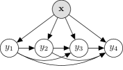
A well-known and well-used baseline approach is to train $L$ binary models, one for each label. This method is called binary relevance (BR); illustrated graphically in Figure 1a. BR classifies an $\mathbf{x}$ individually for each of the $L$ labels, as $h_{BR}(\mathbf{x}):=[h_{1}(\mathbf{x}),\ldots,h_{L}(\mathbf{x})].$

(a)

(b)

Figure 1: BR (1a) and CC (1b) as graphical models, $L=4$. For simplicity, we view $\mathbf{x}=[x_{1},\ldots,x_{D}]$ here as single feature attribute. The arrows represent features being used to predict labels (noting that, a predicted label may be reused as a feature attribute value).

Practically the entirety of the multi-label literature points out that the independence assumption among the labels leads to suboptimal performance (e.g., [7, 18, 1] and references therein), and that for this reason BR cannot achieve optimal performance. A plethora of methods have been motivated by a perceived need to model this dependence and thus improve over BR. Many such methods report a performance improvement over BR, although often at the cost of a computational trade-off. Despite advances in particular contexts, a ‘definitive’ method for modeling dependence has not yet emerged from the literature.

An early approach is that of Meta-BR (MBR, also known variously in the literature as ‘stacked-BR’ and ‘2BR’; [7]) which stacks the output predictions of one BR model as input into a second (meta) BR model, optionally with a skip layer (additionally including the input to both layers), so as to learn to correct the errors of the first model. A related technique is to map infrequent label vector predictions to more frequent label vectors observed in the training data [20] under some distance function (such as Hamming distance). Error-correcting output coding is a similar schema [5].

Rather than ‘correcting’ BR’s predictions, several families of methods attempt to learn and classify the labels together.

The label powerset method (LP, see [24]) is one such family, where each label vector as a single class value in a multi-class problem. The vector chosen as the ‘class label’ is in fact a binary vector indicating label relevances. It can be seen as directly maximizing Eq. (1), where $\mathcal{Y}=\{\mathbf{y}^{(1)},\ldots,\mathbf{y}^{(N)}\}$ (distinct label combinations in the training data). A number of scalable improvements have been made to this approach (RAkEL [25] and HOMER [26] are perhaps two of the most well-known) by dividing up the labelset into a number of smaller more manageable subsets.

Another example is the family of methods based on classifier chains (CC, [19]), illustrated in Figure 1b. This model is related to BR, but uses binary relevance predictions as extra input attributes for the following classifier, cascaded along a chain. In a probabilistic formulation known as probabilistic classifier chains (PCC, [1]), the method can be derived from Eq. (1) simply by expanding the probability distribution under the chain rule, to obtain

$$h_{PCC}(\mathbf{x}):=\operatornamewithlimits{argmax}_{\mathbf{y}\in\{0,1\}}p(y_{1}|\mathbf{x})\prod_{j=2}^{L}p(y_{j}|\mathbf{x},y_{1},\ldots,y_{j-1})$$ (2)

A Bayes-optimal search of the space will provide an optimal solution for Eq. (1). Such a search is exponential with $L$ and thus typically infeasible, but several approximations exist [18, 12, 3]. Arguably the most scalable is the greedy search presented in the original paper, scaling linearly with $L$, and allows writing the prediction as

$$h_{CC}(\mathbf{x}):=\big{[}h_{1}(\mathbf{x}),h_{2}(\mathbf{x},h_{1}(\mathbf{x})),\ldots,h_{L}\big{(}\mathbf{x},h_{1}(\mathbf{x}),\ldots,h_{L-1}(\mathbf{x},h_{1}(\mathbf{x}),\ldots)\big{)}\big{]}$$ (3)

where one can note that the prediction of each base model $h_{j}(\mathbf{x},\ldots)$ only needs to be evaluated once per test instance (and is then used repeatedly along the chain). Each individual classifier may be phrased probabilistically as

$$\hat{y}_{j}=h_{j}(\mathbf{x},\hat{y}_{1},\ldots,\hat{y}_{j-1})=\operatornamewithlimits{argmax}_{y_{j}\in\{0,1\}}p(y_{j}|\mathbf{x},\hat{y}_{1},\ldots,\hat{y}_{j-1})$$ (4)

and thereby we simply obtain predictions in order $\hat{y}_{1},\ldots,\hat{y}_{L}$.

In addition to tractable and approximate search methods for inference, a main focus in the development of CC methods is the order (and more generally, the structure) of the label nodes in the chain. This is often based heavily around an analysis of ‘label dependence’. In fact, at least dozens of variations and extensions have appeared in the literature over the past few years (to add to those already mentioned, [29, 32] are a couple of examples; reviews of many different CC-methods is given in [3, 18]). They have consistently performed strongly in empirical evaluations, however, the reasons for its high performance are only recently being unravelled. In this paper, we throw new light on the subject.

Two common loss measures used in the multi-label literature are Hamming loss,

$$L_{\textsf{Ham}}(\mathbf{y},h(\mathbf{x}))=\frac{1}{NL}\sum_{n=1}^{N}\sum_{j=1}^{L}{\big{[}y_{j}^{(n)}\neq\hat{y}_{j}^{(n)}\big{]}}$$ (5)

and the subset $0/1$ loss:

$$L_{0/1}(\mathbf{y},h(\mathbf{x}))=\frac{1}{N}\sum_{n=1}^{N}{\big{[}\mathbf{y}^{(n)}\neq\mathbf{\hat{y}}^{(n)}\big{]}}$$ (6)

where $[a]=1$ if condition $a$ holds, $\mathbf{\hat{y}}=h(\mathbf{x})$, and $\mathbf{y}=\mathbf{\hat{y}}$ only when both vectors are exactly equivalent. In other words, $0/1$ loss is $1$ wherever Hamming loss is greater than $0$.

From a probabilistic perspective, targeting Eq. (6) results in Eq. (1) (results, e.g., in [2, 18]). This means that both CC and LP are suited to $0/1$ loss, but, whereas CC methods attempt to make a tractable search of $p(\mathbf{y}|\mathbf{x})$ using the chain rule, LP-based methods typically focus on reducing the possible candidates for $\mathbf{y}$ at inference time (i.e., a much-reduced smaller search space $\mathcal{Y}$). There exist many other variations and extensions for this methodology also, but essentially, discussion often focuses on label dependence and modeling labels together.

In this manuscript we more-thoroughly elaborate on earlier arguments (Section 2), and extend them. In particular we compare different views of label dependence; a probabilistic view, and a neural-network view (Section 3). Building on the latter formulation, we create novel methods (Section 4). These methods draw inspiration from neural network methods in the sense of having a hidden layer representation consisting of nodes or units but have the particular advantage that they do not need gradient based learners (e.g., back propagation) to learn the hidden nodes. We achieve this with the idea of ‘synthetic’ labels. The resulting methods obtain a high-performing chain without needing to invest effort in chain ordering (contrasting with the earlier methods that invest much computational power into this step). Our evaluation and discussion of methods and their performance is given in Section 5. Compared to related and competitive methods from the literature, our methods show strong performance on multi-label datasets, and they also provide a strong base for promising future work along the same line. Finally, in Section 6 we summarize and draw conclusions.

2 The Role of Label Dependence in Multi-label Classification

Throughout the multi-label literature the binary relevance method (BR) has been cast out of serious consideration on account of assuming independence among label variables. Substantial empirical evidence has been provided indicating that this method can indeed be outperformed by a margin of several, or even tens of percentage points on standard multi-label datasets.

The main feature of BR that sets it aside from more advanced methods is that it models labels as separate problems, and thus ignores the possible presence of dependence among them. Many dozens of papers have been published over recent years presenting new variations of modeling label dependence, and showing that a proposed method improves over BR.

The underlying idea of much published work is that a model structure based on label dependence will lead to a higher-performance than no structure or than a random structure. A typical recipe is first to count co-occurrence frequencies of labels in the training data, and following this, construct a model based on the dependence discovered. The intuition is that, if two labels occur together frequently (statistically more frequently than would be expected at random), then they should be explicitly modeled. [2] provides us with an excellent summary from a probabilistic point of view, which has become more common on account of supporting a more formal framework in which to define dependence. This naturally includes the idea that two labels which occur less frequently that otherwise expected should also be modeled; implying that human-built topic hierarchies may not necessarily be the best structure (since they tend to separate mutually-exclusive labels into different branches). Probabilistically speaking, in the case of marginal independence, then

$$p(y_{j}|y_{k})\approx p(y_{j})\text{,\quad or equivalently,\quad}p(y_{j},y_{k})\approx p(y_{j})p(y_{k})$$ (7)

for values of some $j$-th and $k$-th labels. This is known as marginal independence, since the input vector ($\mathbf{x}$) is not involved. The distributions $p$ can be approximated by empirical counting in the training set. Given empirical distributions, measures such as mutual information (used in, e.g., [32, 18]) can be calculated. Measuring pairwise marginal dependence is fast even for a large number of labels; and thus is a common choice, e.g., [23, 29].

Models based on marginal dependence may be useful for example for regularizing and ‘correcting’ predictions, as we mentioned in Section 1, but fundamentally a strong argument exists that models should be based on conditional label dependence; since it takes into account the input instance, just as a predictive model does at test time.

Table 2: The toy Logical problem: labels correspond to logical operations on the two-bit input. A dataset is created where each combination is sampled with equal probability or not at all (as shown in the final column).

		or	and	xor
$X_{1}$	$X_{2}$	$Y_{1}$	$Y_{2}$	$Y_{3}$	$P(\mathbf{x},\mathbf{y})$
0	0	0	0	0	$0.25$
0	1	1	0	1	$0.25$
1	0	1	0	1	$0.25$
1	1	1	1	0	$0.25$
…	…	…	…	…	$0$

In Table 2 we introduce a toy example. We may verify (using Eq. (7) for all values $y_{j},y_{k}\in\{0,1\}^{2}$) that labels are marginally dependent. For example for $j,k=2,3$:

$$P(Y_{2},Y_{3}) \neq P(Y_{2})\cdot P(Y_{3})$$

$$[0,0.5,0.25,0.25] \neq[0.37,37.5,0.125,0.125]$$

(where $[p_{1},\ldots,p_{4}]=[P(Y_{1},Y_{2}=0,0),\ldots,P(Y_{1},Y_{2}=1,1)]$ elaborates the distribution). However, in fact in this problem, if we take into account the input, then dependence is absent, for example, if $\mathbf{x}=[0,1]$, then we find that

$$P(Y_{2}|\mathbf{x},Y_{3})=P(Y_{2}|\mathbf{x})=1$$

Results like this motivate models based on conditional dependence. However, obtaining measurements of conditional dependence is particularly intensive, as it inherently involves training classifiers. Indeed, naively $L(L-1)/2$ classifiers should be trained only to obtain pairwise conditional dependence. In [32], an interesting method was proposed that showed how only $L$ binary models need to be trained, then empirically measure the dependence among the errors of the individual models, rather than between labels, as an approximation of measuring conditional dependence. This may not hold rigorously (as explained in [32]) but it is much more efficient. A directed model of nodes is then constructed with off-the-shelf techniques, and a CC employed on it.

Variations of this recipe (of measuring dependence then building a structure then training classifiers) have proliferated in the multi-label literature. However, improvements of predictive performance on standard multi-label datasets have begun to reach a plateau, and usually the top recent methods claiming to leverage label dependence in a particular way will invariably not outperform each other by any significant margin (see, e.g., [15]). Consequently, several authors have begun questioning the implied logic that more technique and computational effort invested in discovering and modeling ground-truth label dependence will lead to better predictive performance versus BR and other methods.

In fact, [2] make the case that it should be possible to make risk-minimizing predictions without any particular effort to detect or model label dependence. In other papers (e.g., [19, 3]) authors ponder if BR has been underrated and could equal the performance of advance methods with enough training data, hence a possible implication that the big data era will render label-dependence models irrelevant. This seems to throw into doubt, or at least under harder scrutiny, the bulk of the contributions to the multi-label literature.

Indeed, in spite of the widely-perceived need to model label dependence, it can sound almost unusual when phrased in everyday terms. Consider an image-labeling task with two labels (say, beach and urban), and two human volunteers each tasked assigning (or not) one of the labels to a set of images. The assumption that CC will outperform BR is analogous to saying that the labeller of beach scenes performs better if having viewed the decisions of the labeller of urban scenes. We would arguably find this surprising, and perhaps even be tempted to question the ability of the beach-scene classifier.

This intuition is correct, if we are to focus only on the beach-scene classifier, and to assume that the task of recognising beaches is independent to recognising urban scenes, having observed the scene itself. Formally: to assume conditional independence and evaluation under Hamming loss. Under these assumptions, if the beach-scene classifier performs better after observing the other’s predictions, it is correct to assume that he/she might actually not be very good at recognising beaches, in spite of the training data, and is perhaps at least partially guessing relevance based on the fact that the presence of urban scenes more likely than not excludes the presence of a beach scene.

This illustrates how the choice of base classifier may affect measured label dependence. And it has an important implication: an ideal structure for predictive performance cannot be obtained only from the data, not even large quantities of data, without consideration of the base classifier. The dependence depends on the base classifier, and thus changing the base classifier will also change the dependency model.

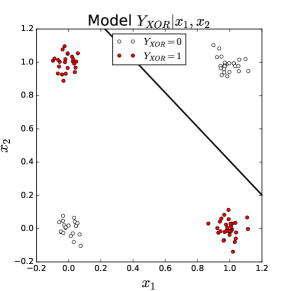
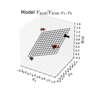
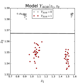
In probabilistic terms, a base classifier may provide us with an approximation of $p(y_{j}|\mathbf{x})$ and $p(y_{j}|\mathbf{x},y_{k})$ (for all label pairs $j,k$, for example), built from the training data. These distributions can be used to measure dependence via Eq. (7). But they may not be a particularly good approximation of the true distributions. In Table 3 we show an example where $p(y_{j}|\mathbf{x},y_{k})\neq p(y_{j}|\mathbf{x})$ if we use off-the-shelf logistic regression but not if we first pass the input through a basis function expansion. Furthermore, if we speak of CC with the original greedy inference, we must take into account that this was not based on a probabilistic setting, and indeed $h_{CC}(\mathbf{x})\neq h_{PCC}(\mathbf{x})$ (see Eq. (2) and Eq. (3)).

Table 3: Results of various methods on the Logical problem (see Table 2 and Figure 4). The base classifier is logistic regression, but BR^(ϕ) first passes the input through a random RBF basis function. The superscripts of (P)CC refer to the models shown in Figure 2. PCC refers to optimal inference; and greedy otherwise.

Metric	BR	CC${}^{\ref{sub@fig:log1}}$	CC${}^{\ref{sub@fig:log2}}$	PCC${}^{\ref{sub@fig:log2}}$	LP	BR(ϕ)
Hamming score	0.83	1.00	0.83	1.00	1.00	1.00
Exact match	0.47	1.00	0.47	1.00	1.00	1.00

Once breaking from a probabilistic graphical framework, the predictive model may lose some connection with the dependence model. This explains why several authors found that to achieve higher accuracy than a random structure, it was necessary to trial a large number of models of different structures via internal validation, and elect the best one (or a top subset) for the final model (as for example in [18]). In this manner, there is no separation between finding structure and building a model, as compared other methods that first model dependence, then build a structure based on it. Unfortunately the cost of trialing many models may be prohibitive for large datasets.

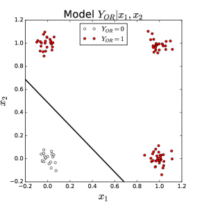
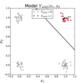
Continuing with the running Logical example (Figure 2, Table 3): Given adequate base models, model 2a (BR) would be sufficient. However, the linear approximation is inadequate and ‘causes’ dependence – in the sense that $h_{\textsc{xor}}$ is functionally dependent on at least one of the other base classifiers under CC (with greedy inference) – and thus only 2c suffices (from the three models shown in Figure 2). This is not true probabilistic dependence, since in that case either 2b or 2c represents the joint distribution probabilistically, and performance with an appropriate inference scheme will be equivalent (shown exactly by PCC in Table 3). The issue is not one of directionality, since a probabilistic directed model has an equivalent indirected model, already experimented in [8] – and relies on costly inference via Gibbs sampling, thus reviving the original tradeoff faced by CC versus PCC. The different structures could be trialed individually (as in [18]), but for any reasonable number of labels, this become challenging.

(a)

(b)

(c)

Figure 2: Models for the Logical toy problem (Table 2): BR (2a) and two initializations of CC (2b, and 2c). Each of these may achieve best accuracy (see also Table 3) depending on base learners and inference schemes.

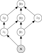
Hence, in consideration of greedy CC, a probabilistic graphical model may give a misleading view. In Figure 3, we draw CC (i.e., Eq. (3)) as a neural network, that fires layerwise from $\mathbf{x}$ to $y_{3}$. Exactly as in CC, $y_{3}$ takes three input features, in this case $[z_{2},y_{2},z_{3}]$ (equivalent to $x,\hat{y}_{1},\hat{y}_{2}$ in CC), and its predictive performance is likely higher than if $y_{3}$ were estimated directly from $x$ (as BR would do).

Figure 3: Classifier chains as a multi-layer neural network. Units $z_{k}$ may be viewed as delay units or simply (and equivalently) as linear hidden units of weight $1$ such that they do not modify the incoming signal. For example, if weights are defined per layer as $\mathbf{w}_{l}$ for the $l$-th layer, then $[z_{1},\hat{y}_{1}]=\mathbf{f}_{1}(\mathbf{w}_{1}^{\top}\mathbf{x})$, $[z_{2},y_{2},z_{3}]=\mathbf{f}_{2}(\mathbf{w}_{2}^{\top}[z_{1},\hat{y}_{1}])$ and $y_{3}=f_{3}(\mathbf{w}_{3}^{\top}[z_{2},y_{2},z_{3}])$. For simplicity, we denote $x=\mathbf{x}$. We assumption that the activation function to $z$-units is linear (and otherwise non-linear). All non-weights are shown as directed arrows, we assume weights from $Z$-units are fixd to $1$, eg., $z_{1}=1\cdot x=x$. Equivalent recurrent versions with self-loops are also possible.

To summarize the above: BR’s often-cited poor performance is not just a result of failing to detect some ground-truth dependence inherent to the data, but may be due to inadequate base models, which induces dependence. A clean separation between the task of measuring label dependence and constructing a model is often not possible due to approximations made for scalability. In this case, connected models compensate for an inadequacy of the individual base classifiers, by augmenting them with additional features (which may in fact be label predictions). In the following section, we discuss how with adequate base models independence can be maintained across outputs, potentially leading to state-of-the-art results.

3 Competitive multi-label classification with independent outputs

In this section we discuss classifiers with independence among the labels. By definition this is a BR classifier, except that in the literature it is assumed that BR connects inputs directly to labels (that there is no hidden layer). We refer to the general case of unconnected labels in the sense that there is no direct connection between any of the outputs; the final prediction for each individual is made independently of other predictions.

We motivate classification using such models, and explain the scenarios where such models should perform at least as well as those of fully-structured models. Namely, we take the view that labels can be independent of each other given a sufficiently powerful inner layer. We discuss existing methods that may be viewed as taking this approach, and we lay the framework for our own approach.

3.1 Motivation for unconnected labels

In the previous section we explain how classifier chains (CC) obtains its performance advantage by using prior labels in the chain as feature-projections for later labels, and that this may compensate for weak or unsuitable base learners (e.g., linear models on non-linear data). Similar conclusions have been separately provided with respect to the label powerset method (LP) in other work, such as [2]: namely, that predictive power comes as a result of working in a higher space. As mentioned above, CC and LP represent many of the popular approaches in the multi-label literature, and lie behind many advanced methods.

Although structured models based on CC and LP methods can provide state-of-the-part performance (some examples: [25, 26, 1, 19]), they nevertheless have some disadvantages: special considerations are necessary to scale up to large numbers of labels, they are often inflexible in the sense of adding/removing labels over time, and have also proved difficult in the past to apply to incremental scenarios such as data streams [17]. A huge number of potential parameterizations and variations of these models requires serious forethought and this can be daunting to practitioners, increasing the temptation to go with the ‘default’ option of BR and build one separate model for each label.

Therefore a binary relevance approach, having no inter-linkage among outputs, remains an attractive option. This is view is already supported by some of the literature. For example, [31] reports that having label-specific features for each label results in a very competitive BR-type classifier.

Most criticism against BR does not involve Hamming loss, since methods predicting labels together (the BR and CC family; which approximate Eq. (1)) target the $0/1$ loss (see Section 1), whereas Hamming loss is optimized precisely by BR (see [2]). However, there is no general need for a particular preference for $0/1$ loss. Hamming loss is a valid and commonly used metric which often coincides with our intuition in many real-world multi-label tasks – namely, when we are interested in the accuracy of each label individually.

Nevertheless, even under exact match, with BR it is empirically possible to outperform structured methods with a suitable base classifier. An example was already illustrated in Figure 4 and Table 3 (where BR outperforms CC under $0/1$ loss by more than twofold, for particular inference schemes and base classifiers).

(a)

(b)

(c)

(d)

(e)

Figure 4: The decision boundaries of base classifiers (logistic regression; shown as black lines/planes) for the three labels of the Logical problem (with some jitter added to the input) of BR (top) and the third label for CC and BR with random basis expansion (in LABEL:sub@f4 and LABEL:sub@f5, respectively). Results are given in Table 3. For simpler visualization, only one link is considered in LABEL:sub@f4. One can see how $h_{3}$ fails in LABEL:sub@f3 (under BR), but succeeds in LABEL:sub@f4 (under CC) and in LABEL:sub@f5 (via BR on the new input space).

3.2 A framework for multi-label classifiers with structural independence among labels

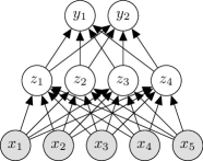
In Figure 3 outputs are independent of each other in each layer. $Y_{1}$ is predicted without knowledge of $Z_{1}$, and so on. Obviously, $Y_{2}$ depends directly on $Y_{1}$, and $Y_{3}$ depends directly on $Y_{2}$ and indirectly on $Y_{1}$ via $Z_{3}$, and thus predictions are obviously not independent. However, note that from the perspective of a neural network, we may write,

$$y_{2} =\mathbf{w}_{2}^{\top}[y_{1},z_{1}]$$

$$=\mathbf{w}_{2}^{\top}[h_{1}(\mathbf{x}),f(\mathbf{x})]$$

$$y_{j} =\mathbf{w}_{j}^{\top}\mathbf{f}(\mathbf{x})=\mathbf{w}_{j}^{\top}\mathbf{z}$$ (8)

Since $h_{1}$ and $f$ are both simply functions on the input, we can say that input units $\mathbf{x}$ produce hidden units $\mathbf{z}$ via activation functions $\mathbf{f}=[f_{1},f_{2}]$ (in the case of $j=2$, then $f_{1}=h_{1},f_{2}=f$) and thus the specific reference to $y_{1}$ disappears from the equation. Under this generalization we could now draw the framework as Figure 5. This is a multi-layer network; with independent (in the sense of unconnected) labels, given a fixed $\mathbf{z}$. The layer $\mathbf{z}=[z_{1},\ldots,z_{H}]$ is not actually ‘hidden’ as would normally be the case in such a representation; but can be seen as a feature transformation of $\mathbf{x}$.

Figure 5: A multi-label neural network with a hidden layer.

We may also arrive at this framework from LP methods. In particular, the well-known RAkEL method [25] extracts $K$ random subsets of the labelset and applies LP to each them; later combining the votes. Let us say that subsets $\{S_{1},\ldots,S_{K}\}$ are chosen where each $S_{k}\subset\{1,\ldots,L\}$, we may consider inner-layer/meta labels $Y_{S_{k}}$ (for $k=1,\ldots,K$). Suppose $S_{k}=\{2,3\}$ (subset of labels $2$ and $3$) which are either both irrelevant or simultaneously relevant to instances the data. Then we could write $Y_{S_{k}}=Y_{\{2,3\}}\in\{[0,0],[1,1]\}$. Assuming that the mapping to the relevant labels is modeled appropriately by the method, we may further simplify notation and simply write $z_{k}\in\{0,1\}$ where (in this case) $y_{\{1,2\}}=[0,0]\Leftrightarrow z_{1}=0$, and $y_{\{1,2\}}=[1,1]\Leftrightarrow z_{1}=1$. Votes for a particular label $y_{j}$ can be decoded deterministically. See an example of two labels depicted in Figure 6. In [25] this is phrased in terms of ensemble voting, but we may generalize this to a sparse vector of weights $\mathbf{w}$ (and bias unit; not shown) and thus write

$$y_{j}=\mathbf{w}_{j}^{\top}\mathbf{z}=\mathbf{w}_{j}^{\top}[z_{1},\ldots,z_{K}]=\mathbf{w}_{j}^{\top}\mathbf{f}(\mathbf{x})$$ (9)

We have recovered again Eq. (8). Only the formation of units $z_{k}$ and the composition of weights $\mathbf{w}$ is different between CC and LP. This difference is arguably considerable, but our main point is to bring the two approaches together under a single framework.

Figure 6: In a RAkEL-like scheme, LP creates different projections via layers in the output space. Note the comparison to Figure 3. We may rename the inner-layer variables to $Z$ to obtain a general representation like that of Figure 5.

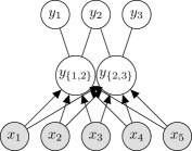
Regarding the performance can we expect from such a framework, this depends on the formation of the inner layer. Empirically, results in the literature show that both greedy-CC and RAkEL-like methods (as represented by this framework) perform strongly across many metrics.

As mentioned, BR is theoretically the best option when outputs are independent [2]. We see that outputs are unconnected in Figure 5 (like BR), yet this general framework encompasses two methods that closely approximate PCC and LP, which in turn optimize $0/1$ loss. The reason is in the inner layer, since if outputs are independent of each other given the input, then minimizing Hamming loss and 0/1 loss is equivalent [2] (recall, these metrics are described in Section 1). This is because, it follows that if labels are independent of each other given the input (complete conditional independence), then Eq. (1) becomes equivalent to

$$\mathbf{\hat{y}} =\operatornamewithlimits{argmax}_{\mathbf{y}\in\{0,1\}^{L}}\prod_{j=1}^{L}p(y_{j}|\mathbf{x})$$

$$=\operatornamewithlimits{argmax}_{\mathbf{y}\in\{0,1\}^{L}}\big{[}p(y_{1}|\mathbf{x})\cdot p(y_{2}|\mathbf{x})\cdot\cdots\cdot p(y_{L}|\mathbf{x})\big{]}$$

$$=[\operatornamewithlimits{argmax}_{y_{1}\in\{0,1\}}p(y_{1}|\mathbf{x}),\ldots,\operatornamewithlimits{argmax}_{y_{L}\in\{0,1\}}p(y_{L}|\mathbf{x})]$$ (10)

which is exactly the (probabilistic) formulation of BR. This suggests that the power lies in the inner-layer representation.

Many loss functions can be used in a neural network in a gradient descent scheme. Back propagation will adjust the weights in the inner layer $\mathbf{z}$ to minimize the loss. Unlike Hamming loss, under $0/1$ loss, the error does not decompose across labels (refer to Eq. (5) and Eq. (6), respectively). Observe that, rewriting Eq. (6), we achieve

$$L_{0/1}(\mathbf{y},\mathbf{\hat{y}}) =\big{[}\mathbf{y}^{(n)}\neq\mathbf{\hat{y}}^{(n)}\big{]}$$

$$=\sum_{\mathbf{y}\in\{0,1\}^{2}}\big{[}\mathbf{\hat{y}}^{(n)}=\mathbf{y}\big{]}p(\mathbf{y}|\mathbf{x})$$

Using this to set up a minimization problem, we recover Eq. (1). In this case, we note that only a single error dimension is back propagated and consequently the network treats the output as a single variable a la LP or PCC with full inference, as discussed earlier.

Yet, despite a non-decomposable loss function, outputs (labels) are still unconnected. They are only connected via input $\mathbf{z}$. The dependence relations are encoded via the inner layer. Hence if using the original input $\mathbf{x}$ does not obtain the required results (high performance given unconnected outputs), we can replace base classifiers or, equivalently, use a powerful $\mathbf{z}$ as input instead, obtained from $\mathbf{z}=\mathbf{f}(\mathbf{x})$. The very important questions remain of how to build $\mathbf{f}$, and what should $\mathbf{z}$ look like given some $\mathbf{x}$. This question has been raised in different points of the literature but has not been definitively answered. Nevertheless, we may at least tackle it. Above we explained how this relates to CC and LP methods, which we will expand on in Section 4. Next, we will review some existing tools and techniques for obtaining powerful latent variables (i.e., an inner layer).

3.3 Existing methods to obtain independence among labels

Although learning latent variable representations is more complex and time consuming than simple input-to-output models, it does provide a means to approach the problem of getting a powerful inner-layer representation. There exists a selection of well-known iterative tools.

One approach to decorrelate labels is to use principle component analysis (PCA) to project from the label space into a new space (of decorrelated labels). This approach was used in, e.g., [22, 28] for multi-label learning. The argument is that if decorrelation is successful, then a BR approach is adequate. Predictions into this new space are then simply cast back into the original label space as predictions. One may use the structure of Figure 5, where $z_{k}$ is the $k$-th principal component. However, the linear decorrelation of PCA is not equivalent to the general concept of obtaining conditional independence. In [28] kernels are used to provide non-linearity, but performance is still dependent on the base classifier since conditional dependence may exist; indeed, since PCA is done only on the label space, the input is not considered.

Expectation maximization (EM) is a useful tool to learn many different types of latent variables (i.e., using different distributions) in an iterative fashion, until below some desired threshold bound. A local maximum will be reached.

The popularity of deep learning furnishes the literature with a number of gradient-based techniques which obtain powerful higher-level feature representations of the data in the form of multiple latent layers of variables and non-linearities, rather than a single hidden layer as was exemplified in Figure 5. These approaches can obtain higher-level abstractions much more more powerful that linear single-layer methods like PCA. Any off-the-shelf method can be used to predict the class label(s) from the top-level hidden layer, or back propagation can be used to fine-tuned all weights for discriminative prediction [10].

Despite recent advances in training, e.g., [4, 21], deep neural networks usually still require careful configuration and parameter tuning and a lot of data, and as such can rarely be seen as an off-the-shelf out-of-the-box method. Training is computationally expensive due to the large number of iterations required to construct the hidden layers. A key point that we emphasise in this paper is that, in multi-label classification we already have a number of such feature representations available: the labels themselves. As we discussed above, both CC and LP-based methods can be viewed as as neural networks with inner layers (illustrated in Figure 3 and Figure 6, respectively). Whether CC or LP can be thought of as ‘deep learning’ is debatable (the features are not learned in a gradient-based fashion, but rather are given as part of the dataset (as labels) more like basis functions). However, the point we wish to make is this: it is a particular advantage to multi-label data that labels may be treated as additional higher-level features, since these features can be learned or simply created, in a supervised fashion.

Later in Section 4.4 we expand the discussion on other methods that can be used for the task of improving the performance of with nodes.

4 Using Labels as Hidden Nodes: Novel Methods and Alternatives

Building on the material and strategies discussed above, we proposed several novel methods, and compare to existing alternatives. These methods use the label space to construct hidden nodes, i.e., inner layers, that augment the predictive power of the method for estimating label outputs.

4.1 Classifier chains augmented with synthetic labels (CCASL)

A common implication of applying CC methods is the search for a good order (or structure) for the labels [12, 18, 14]. If the label representing a difficult concept is at the beginning of the chain, its base learner may fail to learn it and, even worse, propagate this error to the other learners. This problem cannot easily be identified or solved by a superficial dependency analysis (as we explained in Section 2).

Since CC leverages labels as features in higher-dimensional space, it makes sense that more complex (more abstract, higher level) labels are nearer the end of the chain, where they can be predicted using a more complex input space. However, it is not trivial to assess the complexity of each label, and even if it were, it does not help when all labels are quite complex. Thus, we present a method that adds synthetic labels to the beginning of the chain, and builds up a non-linear representation, which can be leveraged by other classifiers further down the chain. We call this Classifier Chains Augmented with Synthetic Labels (CCASL).

Synthetic labels $z_{k}|k=1,\ldots,K$ are created as follows:

$$\mathbf{x}^{\prime}_{k} =[x_{1},\ldots,x_{D},z_{1},\ldots,z_{k-1}]$$

$$\mathbf{w}_{k} =[\mathbf{B}*\mathbf{W}]_{k,1:(D+(k-1))}$$

$$z_{k} =f(\mathbf{w}_{k}^{\top}\mathbf{x}_{k}^{\prime})$$

where $\mathbf{W}$ is a $K\times(D+K-1)$ random weight matrix ($W_{j,k}\sim\mathcal{N}(0,0.2)$) and $\mathbf{B}$ an identically sized masking matrix ($B_{j,k}\sim\textsf{Bernoulli}(0.9)$) such that around 1/10th of weights are zero. A wide selection of activation functions can be selected for $f$. We chose a threshold linear unit (TLU) to make the format of the synthetic labels and true labels both binary, but this is not a requirement. Thus, $z_{k}=f(a_{k})=[a_{k}>t_{k}]$ with randomly-selected threshold $t_{k}\sim\mathcal{N}(\mu_{k},\sigma_{k}\cdot 0.1)$ where $\mu_{k}$ and $\sigma_{k}$ is the empirical mean and standard deviation of values $\{a^{(1)}_{k},\ldots,a^{(N)}_{k}\}$ (the equivalent to standardizing or using an appropriate bias on the middle layer).

In other words, each value $z_{k}$ is projected from input $[x_{1},\ldots,x_{D},z_{1},\ldots,z_{k-1}]$, where each one has a slightly more complex space (expanded by one dimension) than the last. Figure 7 shows the resulting network view. It is not an arbitrary choice that the synthetic labels are placed at the beginning: we want to use these labels to improve prediction of the real labels. We then train CC on label space $\mathbf{y}^{\prime}=[z_{1},\ldots,z_{H},y_{1},\ldots,y_{L}]$ and from the predictions ($\mathbf{\hat{y}}^{\prime}$) we extract the real labels $\mathbf{\hat{y}}=[\hat{y}^{\prime}_{K+1},\ldots,\hat{y}^{\prime}_{K+L}]=[\hat{y}_{1},\ldots,\hat{y}_{L}]$ as the final classification.

As results in Section 5 will show, this method is able to learn the toy Logical dataset perfectly much more often than CC, and does so regardless of the order chosen for the original labels.

Figure 7: Classifier Chains Augmented with Synthetic Labels (CCASL). Random labels $z_{1},\ldots,z_{H}$ are added to the chain prior to the real labels $y_{1},\ldots,y_{L}$. Any CC model can be applied to the top layer.

We also test CCASL on synthetic data, as compared to BR and CC. We create synthetic datasets using a network of random weights and input, ReLU activation functions on the inner layer and TLUs on the output layer; and also simpler datasets without the hidden layer. Having no hidden layer means that only linear decision boundaries are created.

Table 4 shows that the difference between CCASL (with $K=L$ synthetic labels) and BR on the complex synthetic data is significant (nearly 10 percentage points under exact match). The difference between CC and BR is less significant. Conversely, on the simple linear data, CC and CCASL both under-perform BR. This is not surprising, since the use of a cascade is not needed for the simple data, and this leads to overfitting.

Table 4: The average predictive performance of BR, CC and CCASL (with $K=L$) on 150 synthetic datasets of $L=10$ labels, $100$ hidden nodes (only in the case of the complex data) and $N=10000$ examples under 50/50 train/test splits.

	Exact Match	Hamm. Score
BR	0.558	0.843
CC	0.573	0.843
CCASL	0.647	0.867

(a)

	Exact Match	Hamm. Score
BR	0.913	0.967
CC	0.909	0.966
CCASL	0.893	0.959

(b)

Figure 8 displays particular results on smaller dimensions (to visualize easily in a two-dimensional plot). Again we see the contrast in exact match (the results under Figure LABEL:fig:sra1 and Figure LABEL:fig:sra2). CCASL performs relatively much better on the complex data. The accuracy of BR’s base classifiers versus those of CC (in different label orders) sheds some light on this. Under both orders, CC obtains some benefit for the second label, only one of the labels can benefit at a time. Except under CCASL, where both may benefit. Conversely, on the simple synthetic data (two samples of which are given in Figure LABEL:fig:sra8 and Figure LABEL:fig:srb8), CCASL displays no advantage at all over BR, and in fact does worse, exactly as shown in Table 4.

(a)

(b)

(c)

(d)

Figure 8: Illustrative results on synthetic data of dimensions $D=2$, $10$ hidden units (for the complex data), and $L=2$ labels. The legend in the plots indicates $y_{1}y_{2}$. For the complex data generated with a hidden layer (above) we have provided exact match performance of BR, CC (with both possible chain orderings), and CCASL, and also the accuracy of the base classifiers within BR and CC. For the simple data (Figs. LABEL:sub@fig:sra8 and LABEL:sub@fig:srb8) we already know that no dependence exists and thus did not tabulate a similar accuracy analysis.

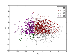
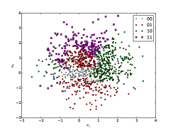
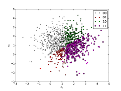
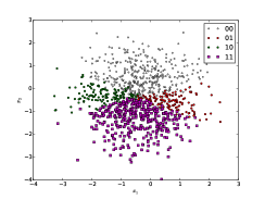
Essentially CCASL creates a cascaded projection of the input space and then combines this space with the label space and learns it together in the style of classifier chains. Scalability is easily tunable by using a smaller and less-cascaded projection (reducing the number of connections). Indeed, it has already been shown that a sparsely connected CC incurrs little to no performance degradation with respect to CC in many cases [29, 18]. But already, relatively few hidden labels are necessary for CCASL; in empirical evaluation we obtain good performance with $K=L$.

4.2 Adding a meta layer: CCASL+BR

In spite of solving the Logical problem and excelling on synthetic data, our empirical results (in Section 5) show that CCASL does not appear to out-perform CC by much on real datasets. Besides this issue, we already stated a desire for models that have an unconnected label layer. To obtain the independent outer layer and also counteract overfitting, we also add an extra BR-layer (i.e., a meta-BR) to get CCASL+BR. Figure 9 displays the resulting network.

Figure 9: CCASL+BR: CCASL as a middle layer. Outputs are stacked again into a second meta BR-classifier (i.e., similarly to MBR). By modeling dependence in the middle layer, dependence can be ignored in the output layer.

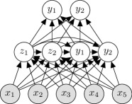
CCASL+BR combines the advantages of several important methods in the multi-label literature: namely BR (outputs are not directly connected to each other), MBR (a form of regularization), and CC (a chain cascade to add predictive power). Back propagation is not necessary.

A potentially interesting alternative to the issues faced by CCASL is to reconsider a more thorough probabilistic inference, to avoid error propagation (itself a kind of overfitting). We leave a detailed investigation to future work, but do include an experimentation of this approach in Section 5.

4.3 Adding an augmented layer of meta labels: CCASL+AML

In addition to creating synthetic labels from the feature space, it is also possible to create synthetic labels from the label space, as we outlined in Section 3. Namely, we create binary synthetic labels, based on subsets $S_{k}\subset\{1,\ldots,L\}$. For each such subset, the most common combination $\mathbf{y}^{*}_{S_{k}}$ is selected from the training data. This allows us to create binary variables

$$z_{k}=\big{[}\mathbf{y}_{S_{k}}=\mathbf{y}_{S_{k}}^{*}\big{]}$$

where, as used above, the notation $\big{[}a\big{]}$ returns $1$ if condition $a$ holds (else $0$).

To re-exemplify, if we select $S_{k}=\{1,3,6\}$, and if we find that the most commonly occurring combination of these labels in the training set is $\mathbf{y}_{S_{k}}^{*}=\mathbf{y}^{*}_{\{1,3,6\}}=[1,0,1]$, then $z_{k}=1$ indicates the relevance of this combination, and $1/K$ votes are added to $y_{1}$, $y_{3}$, and $y_{6}$.

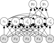
For even more predictive power, we combine these units with synthetic labels generated from the feature space, as does CCASL, and hence denote this method CCASL+AML (CCASL with an Augmented Meta/middle Layer). The resulting network is exemplified in Figure 10. In the figure, we distinguish the AML units as $z^{\prime}_{k}$ from the CCASL units as $z_{k}$.

Figure 10: CCASL with an Augmented Middle Layer (CCASL+AML). The prime distinguishes the meta labels $z^{\prime}_{k}$ from the synthetic cascaded labels $z_{k}$ (in this illustration).

4.4 Related and alternatives models

Adding non-linearity to an otherwise linear method via basis expansions is a fundamental technique in statistical learning [9]. Under this methodology, basis functions can be either chosen suitably by a domain expert, or simply chosen arbitrarily to achieve a more dimensioned representation of the input, and higher predictive performance. In this latter case, polynomials are a common choice, such that $\mathbf{z}=x^{2},x^{3},\ldots,x^{p}$ up to some degree $p$. Under this approach learning can proceed ordinarily by treating $\mathbf{z}$ as the input.

Restricted Boltzmann machines (RBMs) are a probabilistic method for finding higher-level feature representations $\mathbf{z}=f(\mathbf{W}^{\top}\mathbf{x})$, where $\mathbf{W}$ is learned with gradient-based methods such as to minimize energy $E(\mathbf{x},\mathbf{y},\mathbf{z})=\exp\{-\mathbf{z}^{\top}\mathbf{W}\mathbf{x}\}$ and $f$ is some non-linearity (typically a sigmoid function $f(a)=\frac{1}{1+e^{-a}}$, but more recently ReLUs have been particularly popular). The RBM can then cast any input instance stochastically into a different-dimensioned space, as $\mathbf{z}$. Any classifier (e.g., BR) can be trained on this space. The RBMs are often stacked on each other greedily and fine tuned for discriminative classification with back propagation [10] but can also be trained directly for competitive discriminative prediction [13].

The multi-layer multi-label neural-network ‘BPMLL’ proposed earlier by [33] has become well known in the multi-label literature. Its structure is essentially that exemplified in Figure 5, and the hidden layer is trained using back propagation. The only difference from a vanilla multi-layer perceptron (MLP) is that it is trained to minimize a rank loss. However, its out-of-the-box performance has consistently been shown to under-compete with the state-of-the-art. Later, a multi-label radial-basis-function (RBF) network was proposed by [30]. However, this network was not picked up widely in the literature. The limited reception of these methods is possibly due to the fiddly ‘hit-and-miss’ nature of the gradient-based learning (with respect to the selection of learning rates, hidden nodes and so on) which we have specifically tried to avoid with our methods.

Recently, [16] readdressed the application of neural networks for multi-label classification, in particular for the task of large scale text classification. They implemented MLPs with a number of recently proposed techniques from deep learning, namely ReLUs, AdaGrad, and dropout. They also used the standard cross entropy loss function and sigmoid activations functions, as opposed to BPMLL’s choice of rank loss. At least on text datasets (the particular domain they tackled) these networks were shown to be highly competitive compared to BPMLL.

Even with the latest techniques, the primary disadvantage often associated with multi-layer neural networks is that of back propagation, which is widely used for discriminative learning, involving many iterations of propagating the input up through the network to the outputs and then the error back down to adjust the weights. This is the case even for stacked deep networks with RBMs for pre-training weights. Indeed, for this reason [16] build a case for only using no more than a single hidden layer (despite using the latest deep-learning techniques) on their large datasets.

An early alternative to back propagation in neural networks was proposed by [27], to use the idea of random functions to project the input layer into a new space in the hidden layer, rather than learn this hidden layer iterative gradient descent. More recently, this idea has appeared in so-called ‘extreme learning machines’ (ELMs, [11]), which are essentially neural networks with random weights. Again, this is built on the premise of eliminating the need for gradient-based methods in the hidden layer to obtain huge speed ups in learning. Radial basis functions are a typical choice in ELMs, making them closely related to (or in fact, an instance of) RBF networks (e.g., [30]). ELMs are related to the methods we propose. However, unlike CCASL+AML, ELMs do not work down from the label layer. Furthermore, in our approach we use a cascade of functions which are treated as synthetic labels and learned in a supervised manner along with the real labels.

Some methods transform the label space, and predict into this space, thus being related to our methods. Already (in Section 3.3) we mentioned principal label-space transformation [22] and variations [28] that make the independent targets, apply independent models to them, and then cast the predictions back into the original label space. The various methods used (such as PCA) are related to RBMs via factor analysis (RBMs can be seen as a binary version thereof).

Many methods for obtaining latent variables can be cast in a probabilistic graphical model framework (for example RBMs). Already in [3], parallels are drawn between probabilistic CC and conditional random fields (CRFs), which are a general class of latent-variable model. CRFs have been studied with application to multi-label classification by [6]. But as discussed earlier, greedy CC is more comparable to explicit basis function and loses some of its probabilistic connections and is difficult to cast into the indirected nature of a CRF.

Finally, simply using a powerful non-linear base classifier may remove the need for transformations of the feature space altogether. For example, decision trees are non-linear classifiers that have proven themselves in a huge variety of domains, including in multi-label classification, as shown in [15].

5 Experiments

We conducted an empirical evaluation on a variety of multi-label datasets commonly used in the literature, comparing to established baseline and related methods from the literature. The main goals are to compare relative performance of our proposed methods under different dataset/metric combinations and to investigate the mechanisms behind this performance.

5.1 Setup and methodology

We compare the novel methods that we developed (namely, CCASL and variants) with a selection of methods from the literature: baseline BR, CC both with greedy inference, and with Monte-Carlo search for inference (the latter we refer to as PCC), an ELM, and a MLP. Table 5 summarizes methods and their parameters. References and descriptions can be found in Section 1 and Section 4.4. For base classifiers, we used logistic regression in all cases (including ELMs and MLP in the sense that the final layer of these networks uses sigmoid activation functions), except when denoted with a superscript RF which denotes random forest as a base classifier (e.g., BR_RF). All methods were implemented in Python, using the Scikit-Learn library for logistic regression and random forest.

Table 5: Summary of methods. We propose the ones based on CCASL.

Method	Strategy	Parameters
BR	Independent outputs
CC	Cascade across labels
PCC	…with Monte-Carlo inference	$M=50$ iterations/example
CCASL	CC with synthetic labels	$K=L$
CCASL+MBR	…as input to a BR	$K=L$
CCASL+AML	…with additional meta labels	$K=L,K^{\prime}=2L^{\dagger},|S_{k}|=3$
ELM	Random projection to BR	$K=2L$, TLU activation
BRRF	BR with random forest
MLP	Neural network with back prop.	$K\in\{2L,2D\}^{\ddagger},\lambda=0.1,I=1000$,
		sigmoid activation

†	$K^{\prime}$ is the number of AML units; each based on random subset $S_{k}\subseteq\{1,\ldots,L\}$
‡	Best of these (on internal 60/40 split), but limited to maximum $K=100$

We used 10 datasets typically used in multi-label evaluations, plus a version of the illustrative logical dataset from Section 3. All are listed in Table 6.

Table 6: A collection of datasets and associated statistics, where LC is label cardinality: the average number of labels relevant to each example.

	$N$	$L$	$D$	LC	Type
Logical	20	3	2	1.50	logical
Music	593	6	72	1.87	audio
Scene	2407	6	294	1.07	image
Yeast	2417	14	103	4.24	biology
Medical	978	45	1449	1.25	medical/text
Enron	1702	53	1001	3.38	text
Reuters	6000	103	500	1.46	text
OHSUMED	13929	23	1002	1.66	text
MediaMill	43907	101	120	4.38	video
Bibtex	7395	159	1836	2.40	text
Corel5k	5000	374	499	3.52	image

We use the score metrics (higher values are better): Hamming score (the score equivalent of Hamming loss; Eq. (5)), and exact match (the score equivalent of $0/1$ loss; Eq. (6)), already detailed in this paper and used extensively in multi-label evaluations. Hamming score rewards methods for predicting individual labels well, whereas exact match rewards a higher proportion of instances with all label relevances correct.

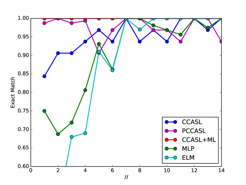
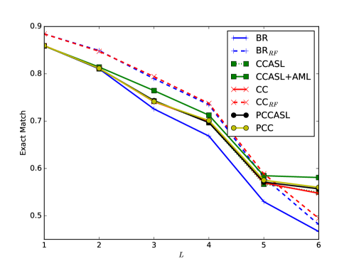
We carry out 10 iterations for each dataset, each time with a random 60/40 train-test split and a random order of labels. Figure 11 shows the effect of different numbers of synthetic labels / hidden nodes for performance on the Logical dataset. Figure 12 shows the effect of more or fewer output labels given an equivalent input space. Table 7 shows the main results, of predictive performance across all datasets. Table 8 shows the results in terms of running time. All experiments were run on Intel 2.6 GHz processors.

Figure 11: Different methods compared on the Logical dataset for varying numbers of hidden nodes. Each point represents the average of 10 runs on 60/40 train/test split with randomly shuffled labels. Note that PCCASL refers to CCASL with probabilistic Monte-Carlo inference (as used in PCC in the other experiments); 10 iterations/example in this case.

Table 7: Predictive performance in terms of exact match and Hamming score. Average result across $10$ randomizations (of instance and label space) and a 60/40 train/test splits. The average rank is shown after the performance for each dataset. Value rounded to 2dp and rank rounded to 1dp for display only. CCASL+ is abbreviated to C.+.

Dataset	BR	CC	PCC	CCASL	C.+BR	C.+AML	ELM	BRRF	MLP
Logical	0.52 9	0.64 8	0.87 4	0.78 7	1.00 2	1.00 2	0.79 6	1.00 2	0.83 5
Music	0.23 8	0.25 6	0.26 2	0.25 4	0.26 3	0.27 1	0.17 9	0.25 7	0.25 4
Scene	0.47 8	0.55 5	0.56 3	0.54 6	0.56 4	0.58 1	0.21 9	0.48 7	0.56 2
Yeast	0.14 6	0.18 2	0.19 1	0.18 3	0.17 5	0.18 4	0.11 8	0.10 9	0.12 7
Medical	0.45 7	0.46 6	0.42 8	0.68 3	0.70 1	0.69 2	0.28 9	0.68 4	0.62 5
Enron	0.11 7	0.12 5	0.12 4	0.13 2	0.13 2	0.13 1	0.06 9	0.12 6	0.09 8
Reuters	0.45 7	0.47 4	0.47 1	0.47 6	0.47 2	0.47 2	0.37 9	0.47 5	0.38 8
Ohsumed	0.15 4	0.15 3	0.15 4	0.15 7	0.15 7	0.15 6	0.03 9	0.17 2	0.21 1
M.Mill	0.09 8	0.12 3	0.12 4	0.13 1	0.11 6	0.11 5	0.10 7	0.12 2	0.05 9
Bibtex	0.10 5	0.11 4	0.10 6	0.17 1	0.16 3	0.17 2	0.04 9	0.10 7	0.07 8
Corel5k	0.01 7	0.01 4	0.00 9	0.02 3	0.02 1	0.02 1	0.01 7	0.01 5	0.01 7
avg rank	6.95	4.55	4.23	4.05	3.45	2.55	8.27	5.09	5.86

(a)

Dataset	BR	CC	PCC	CCASL	C.+BR	C.+AML	ELM	BRRF	MLP
Logical	0.84 8	0.88 7	0.96 4	0.93 6	1.00 2	1.00 2	0.93 5	1.00 2	0.06 9
Music	0.79 2	0.78 7	0.78 6	0.78 7	0.78 5	0.78 4	0.75 9	0.79 1	0.78 3
Scene	0.87 8	0.88 6	0.88 4	0.88 7	0.88 4	0.88 3	0.84 9	0.90 1	0.89 2
Yeast	0.79 1	0.78 6	0.78 8	0.78 7	0.78 4	0.78 5	0.79 3	0.79 2	0.22 9
Medical	0.70 9	0.72 7	0.72 8	0.95 6	0.98 2	0.98 3	0.96 5	0.99 1	0.98 4
Enron	0.90 8	0.92 6	0.91 7	0.94 3	0.94 3	0.94 2	0.93 5	0.95 1	0.07 9
Reuters	0.98 9	0.98 7	0.98 7	0.99 4	0.99 2	0.99 2	0.98 5	0.99 1	0.98 5
Ohsumed	0.92 4	0.92 5	0.92 6	0.92 8	0.92 8	0.92 8	0.93 3	0.94 1	0.93 2
M.Mill	0.97 2	0.97 6	0.97 8	0.97 6	0.97 4	0.97 4	0.97 4	0.97 1	0.96 9
Bibtex	0.98 6	0.98 5	0.98 7	0.99 2	0.99 2	0.99 2	0.97 9	0.99 2	0.98 7
Corel5k	0.98 7	0.98 5	0.97 9	0.98 4	0.99 2	0.99 2	0.98 5	0.99 1	0.98 8
avg rank	5.82	6.27	6.86	5.64	3.68	3.50	5.73	1.32	6.18

(b)

5.2 Discussion

Results highlight the performance of CCASL methods. All out-perform baseline BR and CC overall, particularly with meta layers (+BR and +AML). Under exact match, the CCASL+ methods are almost invariably the top performers. There are some exceptions – under Yeast and Ohsumed – with respect to P/CC. Already it has been observed that that advanced methods typically do not make any significant improvements over each other or BR on the Yeast dataset (see, for example, the results of [15]) and indeed we note that under Hamming score, it is BR that obtains the top score. On Ohsumed the difference is not distinguishable even at two decimal places. PCC performs competitively overall (indeed, the gains of CASSL methods are marginal in many cases), but at a cost of being one of the slowest method in evaluation, on account of more costly inference; (although as mentioned earlier, there are other inference methods exist for PCC, and these may be faster, e.g., [3]). Interestingly, the best performance against PCC was obtained on text datasets.

Possibly, higher results could be obtained from the MLPs with more exhaustive parameter tuning. However, the need for such tuning is an issue in itself; we already tried several different parameter combinations. Furthermore, running time (Table 8) is already an order of magnitude (or more) higher than CCASL methods due to their iterative learning procedure. An important advantage of the synthetic nodes is eliminating the need for such procedures.

Under Hamming score, BR_RF clearly performs best. This is in line with our earlier discussion, since random forests are powerful non-linear models, and as such are able to ensure that base learners perform well independently under this metric. This is the case to some extent with CCASL (which also performs very well under this metric), but in some particular cases, BR_RF is more successful.

Figure 11 confirms that, while established methods such as MLP and ELM can also learn difficult concepts (such as the xor label, as widely known in the literature), in practice they need more hidden nodes as compared to our proposed CCASL methods. In fact, even a single hidden nodes is enough for CCASL+AML. Using PCC-inference (PCCASL) leads to near-perfect performance with small $K$, however, performance actually decreases, or at least becomes more unstable, with larger $K$. The explanation for this is that the number of iterations for MCC is held constant, but the search space increases exponentially with $K$ (namely, $2^{(3+K)}$). More Monte-Carlo iterations will help (indeed, 10 is arguably low), at a computational cost, but the trend is already clear.

The performance improvement of several of the methods (including CCASL and BR_RF) over BR and CC on Medical is considerable. A closer look revealed that individual label accuracy increases along CC’s chain from roughly $0.67$ to $0.75$, and from $0.93$ to $0.99$ in CCASL’s chain (excluding the synthetic labels), clearly showing the effect of using synthetic labels first. We already managed to reproduce similar differences on synthetic data (Table LABEL:fig:srb8) and, of course, the Logical dataset.

The gap in running times becomes noticeable under the large datasets, where CCASL methods are around twice as expensive as BR/CC. However, if the extra time was used for trialling chain orders with internal train/test split for CC, it is probably not enough to make up the gap in predictive performance. BR_RF is also competitively fast. Tree-based methods for multi-label classification also proved themselves in a similar way in [15].

Table 8: Average Running Time (seconds) and ranking across $10$ train/test splits.

Dataset	BR	CC	PCC	CCASL	C.+BR	C.+AML	ELM	BRRF	MLP
Logical	0 1	0 1	0 8	0 3	0 5	0 6	0 3	0 7	1 9
Music	0 4	0 3	2 8	0 5	0 6	0 7	0 1	0 2	48 9
Scene	1 4	1 3	10 8	2 5	2 6	3 7	0 1	0 2	244 9
Yeast	0 2	0 3	33 8	1 5	2 6	3 7	0 1	1 4	114 9
Medical	5 3	5 4	31 8	12 5	12 6	13 7	0 2	0 1	243 9
Enron	19 3	20 4	85 8	37 5	38 6	41 7	1 2	1 1	965 9
Reuters	129 3	141 4	430 8	338 6	328 5	359 7	50 2	30 1	1555 9
Ohsumed	236 3	269 4	478 7	379 5	607 8	394 6	22 1	58 2	3081 9
M.Mill	426 2	410 1	3753 8	904 3	1062 6	1048 5	908 4	2295 7	5830 9
Bibtex	1535 3	1616 4	1934 5	3372 6	3411 7	3440 8	141 2	60 1	6766 9
Corel5k	464 3	566 4	2210 9	1311 5	1423 6	1562 7	309 2	142 1	1747 8
avg rank	2.86	3.23	7.73	4.86	6.09	6.73	1.95	2.64	8.91

Chaining mechanisms can obtain a greater advantage on datasets with more labels, simply because these labels can be leveraged for a more powerful predictive structure for other labels. Figure 12 illustrates this on the Scene data, where the label variables are incrementally added. For predicting a single label (corresponding to binary classification), random forest clearly outperforms logistic regression. On the other hand, with all six labels, CC-based methods with logistic regression actually performs better, with CCASL+AML performing best, followed by others. Notice that the chaining mechanism does not particularly help with random forests – only a minor improvement of CC_RF over BR_RF is obtained with more labels. The performance signal of CCASL+AML separates from other CC-logistic methods at only the second label, whereas the difference between CC and PCC only becomes noticeable at around $L=5$ or $L=6$. On this particular dataset the performance of CCASL and PCC is virtually indistinguishable, as already observable in Table 7a. Using probabilistic inference (PCCASL) suggests a marginal improvement in this case. The biggest separation in the performance signal is greatest at $L=6$, but does not grow consistently or linearly amoung all methods, indicating again that it is not just the number of labels but also the inherent complexity of each label that affects performance of different methods.

Figure 12: Different methods compared on the Scene dataset for varying numbers of output labels. For example, where $L=3$ then only the first $3$ labels of the dataset are considered for learning and evaluation. As in the above experiments $RF$ indicates that random forest was the base learner; in other cases it is logistic regression. As in Figure 11, PCCASL is CCASL with Monte-Carlo sampling inference.

Our proposed methods showed an advantage in terms of overall ranking and in many particular dataset/metric combinations, however the main goal of the paper was to further investigate and detail the underlying mechanisms responsible for good performance, and in particular the use of labels as hidden nodes. Results indicate the utility of this mechanism. A multi-layer neural network structure is theoretically also as capable as our methods (in terms of approximation ability), however results highlighted the fact that they are difficult to employ in an out-of-the-box fashion. Both approaches use hidden nodes, but it is faster and much easier to use ‘synthetic labels’ than to train a standard back-propagation neural network (MLP), and also much more effective than a random-projection neural network (ELM).

We reiterate that it is generally not possible to say that a particular classifier is overall advantageous across all possible scenarios. It was also apparent in our results that different classifiers performed better on certain datasets and under different evaluation metrics: a non-linear decision tree classifier is preferable to logistic regression as a base classifier on Ohsumed and MediaMill, and for several datasets under Hamming loss, but in many other contexts, a linear base learner can be more successfully employed in a classifier-chain or hidden-node classifier.

In this paper we examined in particular Hamming score and exact match. Dozens of metrics, including for example the micro- and macro-averaged F1 measures, have been used in the literature. A full comparison is outside the scope of this paper, but large-scale empirical comparisons (e.g., [15]) indicate that methods that perform well on both Hamming score and exact match also tend to perform well across a range of other metrics.

Perhaps it is also worth remarking that there are now a plethora of multi-label methods, and parameter configurations thereof. Comparing to all of them is outside the scope and possibility of this work, however, future comparisons will help further unravel the mechanisms behind the successful methods, and the contexts wherein this success is most likely to occur.

6 Summary and Conclusions

Many methods for multi-label classification measure label dependence in a dataset and then use this information to build structured models with cases of significant dependence manifested explicitly as direct connections among the label outputs. These methods have performed well in the literature in empirical evaluations, but understanding of their mechanism has lagged behind these results. We have contributed to the analysis in this area and looked into this mechanism in greater depth. A common view is that models should be built on a structure that approximates an underlying ground-truth structure in the data. Although in a strict probabilistic sense this may be the case, in practice many shortcuts are taken to deal with scalability concerns, and we explained how in many cases modeling dependence among outputs is simply compensating for an inadequate base classifier or inference scheme, and labels are being leveraged as advanced feature-transformations. We exploited this mechanism in an inner layer, creating efficient methods that perform well even with unconnected labels at the outer layer, and even with a simple linear base learner, one can still obtain competitive results in this manner.

We proposed several methods based on the idea of inner ‘synthetic labels’, with different combinations of the labels, both in a cascade form from the features and label subset-composition from the label space. This is not possible in traditional single-label classification where a single target is predicted for each instance. Leveraging the synthetic labels means that our methods do not need gradient-based back propagation to train inner nodes: multiple levels are created instantly from combinations of input and output. The methods we presented outperformed a variety of related algorithms. In future work, we intend to investigate the output of combining this methodology of synthetic labels to speed up existing gradient descent algorithms.

7 Acknowledgements

This work was supported in part by the Aalto Energy Efficiency Research Programme (http://aef.aalto.fi/en/), and Academy of Finland grant 118653 (ALGODAN).

References

- [1] Krzysztof Dembczyński, Weiwei Cheng, and Eyke Hüllermeier. Bayes optimal multilabel classification via probabilistic classifier chains. In ICML ’10: 27th International Conference on Machine Learning, pages 279–286, Haifa, Israel, June 2010. Omnipress.
- [2] Krzysztof Dembczyński, Willem Waegeman, Weiwei Cheng, and Eyke Hüllermeier. On label dependence and loss minimization in multi-label classification. Mach. Learn., 88(1-2):5–45, July 2012.
- [3] Krzysztof Dembczyński, Willem Waegeman, and Eyke Hüllermeier. An analysis of chaining in multi-label classification. In ECAI: European Conference of Artificial Intelligence, volume 242, pages 294–299. IOS Press, 2012.
- [4] John Duchi, Elad Hazan, and Yoram Singer. Adaptive subgradient methods for online learning and stochastic optimization. J. Mach. Learn. Res., 12:2121–2159, July 2011.
- [5] Chun-Sung Ferng and Hsuan-Tien Lin. Multi-label classification with error-correcting codes. In Proceedings of the 3rd Asian Conference on Machine Learning, ACML 2011, Taoyuan, Taiwan, November 13-15, 2011, pages 281–295, 2011.
- [6] Nadia Ghamrawi and Andrew McCallum. Collective multi-label classification. In CIKM ’05: 14th ACM international Conference on Information and Knowledge Management, pages 195–200, New York, NY, USA, 2005. ACM Press.
- [7] Shantanu Godbole and Sunita Sarawagi. Discriminative methods for multi-labeled classification. In PAKDD ’04: Eighth Pacific-Asia Conference on Knowledge Discovery and Data Mining, pages 22–30. Springer, 2004.
- [8] Yuhong Guo and Suicheng Gu. Multi-label classification using conditional dependency networks. In IJCAI ’11: 24th International Conference on Artificial Intelligence, pages 1300–1305. IJCAI/AAAI, 2011.
- [9] Trevor Hastie, Robert Tibshirani, and Jerome Friedman. The Elements of Statistical Learning. Springer Series in Statistics. Springer New York Inc., New York, NY, USA, 2001.
- [10] Geoffrey Hinton and Ruslan Salakhutdinov. Reducing the dimensionality of data with neural networks. Science, 313(5786):504 – 507, 2006.
- [11] Guang-Bin Huang, DianHui Wang, and Yuan Lan. Extreme learning machines: a survey. International Journal of Machine Learning and Cybernetics, 2(2):107–122, 2011.
- [12] Abhishek Kumar, Shankar Vembu, AdityaKrishna Menon, and Charles Elkan. Beam search algorithms for multilabel learning. Machine Learning, 92(1):65–89, 2013.
- [13] Hugo Larochelle, Michael Mandel, Razvan Pascanu, and Yoshua Bengio. Learning algorithms for the classification restricted Boltzmann machine. J. Mach. Learn. Res., 13:643–669, March 2012.
- [14] Weiwei Liu and Ivor Tsang. On the optimality of classifier chain for multi-label classification. In C. Cortes, N. D. Lawrence, D. D. Lee, M. Sugiyama, and R. Garnett, editors, Advances in Neural Information Processing Systems 28, pages 712–720. Curran Associates, Inc., 2015.
- [15] Gjorgji Madjarov, Dragi Kocev, Dejan Gjorgjevikj, and Sašo Džeroski. An extensive experimental comparison of methods for multi-label learning. Pattern Recognition, 45(9):3084–3104, September 2012.
- [16] Jinseok Nam, Jungi Kim, Eneldo Loza Mencía, Iryna Gurevych, and Johannes Fürnkranz. Large-scale multi-label text classification - revisiting neural networks. In ECML-PKDD ’14: 25th European Conference on Machine Learning and Knowledge Discovery in Databases, pages 437–452, 2014.
- [17] Jesse Read, Albert Bifet, Geoff Holmes, and Bernhard Pfahringer. Scalable and efficient multi-label classification for evolving data streams. Machine Learning, 88(1-2):243–272, 2012.
- [18] Jesse Read, Luca Martino, and David Luengo. Efficient Monte Carlo methods for multi-dimensional learning with classifier chains. Pattern Recognition, 47(3):1535–1546, 2014.
- [19] Jesse Read, Bernhard Pfahringer, Geoffrey Holmes, and Eibe Frank. Classifier chains for multi-label classification. Machine Learning, 85(3):333–359, 2011.
- [20] Robert E. Schapire and Yoram Singer. Improved boosting algorithms using confidence-rated predictions. Machine Learning, 37(3):297–336, December 1999.
- [21] Nitish Srivastava, Geoffrey Hinton, Alex Krizhevsky, Ilya Sutskever, and Ruslan Salakhutdinov. Dropout: A simple way to prevent neural networks from overfitting. Journal of Machine Learning Research, 15:1929–1958, 2014.
- [22] Farbound Tai and Hsuan-Tien Lin. Multilabel classification with principal label space transformation. Neural Comput., 24(9):2508–2542, September 2012.
- [23] Lena Tenenboim, Lior Rokach, and Bracha Shapira. Identification of label dependencies for multi-label classification. In MLD ’10: 2nd International Workshop on Learning from Multi-Label Data from ICML/COLT 2010, 2010.
- [24] Grigorios Tsoumakas and Ioannis Katakis. Multi label classification: An overview. International Journal of Data Warehousing and Mining, 3(3):1–13, 2007.
- [25] Grigorios Tsoumakas, Ioannis Katakis, and Ioannis Vlahavas. Random k-labelsets for multi-label classification. IEEE Transactions on Knowledge and Data Engineering, 23(7):1079–1089, 2011.
- [26] Grigorios Tsoumakas, Ioannis Katakis, and Ioannis P. Vlahavas. Effective and efficient multilabel classification in domains with large number of labels. In ECML/PKDD Workshop on Mining Multidimensional Data, 2008.
- [27] W. Thomas Miller III, Filson H. Glanz, and L. Gordon Kraft III. CMAC: An associative neural network alternative to backpropagation. Proceedings of the IEEE, 78(10):1561–1567, October 1990.
- [28] Jason Weston, Olivier Chapelle, André Elisseeff, Bernhard Schölkopf, and Vladimir Vapnik. Kernel dependency estimation. In Advances in Neural Information Processing Systems 15 (NIPS), pages 897–904, 2003.
- [29] Julio H. Zaragoza, Luis Enrique Sucar, Eduardo F. Morales, Concha Bielza, and Pedro Larrañaga. Bayesian chain classifiers for multidimensional classification. In 24th International Joint Conference on Artificial Intelligence (IJCAI ’11), pages 2192–2197, 2011.
- [30] Min-Ling Zhang. ML-RBF : RBF neural networks for multi-label learning. Neural Processing Letters, 29(2):61–74, 2009.
- [31] Min-Ling Zhang and Lei Wu. Lift: Multi-label learning with label-specific features. Pattern Analysis and Machine Intelligence, IEEE Transactions on, 37(1):107–120, Jan 2015.
- [32] Min-Ling Zhang and Kun Zhang. Multi-label learning by exploiting label dependency. In KDD ’10: 16th ACM SIGKDD International conference on Knowledge Discovery and Data mining, pages 999–1008. ACM, 2010.
- [33] Min-Ling Zhang and Zhi-Hua Zhou. Multilabel neural networks with applications to functional genomics and text categorization. IEEE Transactions on Knowledge and Data Engineering, 18(10):1338–1351, 2006.