Abstract

We show that there exists the inverse Kibble-Zurek scenario, when we start with an equilibrium system with broken symmetry and, by imposing perturbations, transform it to a strongly nonequilibrium symmetric state through the sequence of states with spontaneously arising topological defects. We demonstrate the inverse Kibble-Zurek scenario both experimentally, by perturbing the Bose-Einstein condensate of trapped ⁸⁷Rb atoms, and also by accomplishing numerical simulations for the same setup as in the experiment, the experimental and numerical results being in good agreement with each other.

Keywords: Nonequilibrium Bose gas; Quantum vortices; Vortex turbulence; Grain turbulence, Wave turbulence; Inverse Kibble-Zurek scenario

Corresponding author: V.I. Yukalov,
Address: Bogolubov Laboratory of Theoretical Physics,
Joint Institute for Nuclear Research, Dubna 141980, Russia.
Phones: 7(496)216-3947; 7(496)213-3824
E-mail: yukalov@theor.jinr.ru

1 Introduction

The Kibble-Zurek mechanism [1, 2, 3, 4, 5] characterizes the spontaneous formation of defects in the process of system equilibration from an initial strongly nonequilibrium symmetric state to an equilibrium state with broken symmetry. This is a very general mechanism illustrated by numerous examples ranging from various condensed-matter systems to cosmological objects [2, 4, 5]. It has been experimentally observed, in ion crystals [6, 7], superconducting films [8], superfluid ³He and superfluid ⁴He, modeling cosmological string formation [9, 10, 11], in trapped atoms exhibiting Bose-Einstein condensation [12, 13], and in a homogeneous Bose gas [14].

The case of nonequilibrium Bose-Einstein condensation in dilute Bose gases has attracted special attention since the work by Levich and Yakhot [15] followed by many other publications studying, both theoretically [16, 17, 18] and in computer simulations [19, 20, 21], the process of equilibration of an uncondensed system to its Bose-condensed state. The general understanding of the process of this equilibration, passing through the states with topological defects, is as follows.

One starts with a strongly nonequilibrium state possessing no Bose-Einstein condensate, which is termed wave turbulence or weak turbulence. In the process of equilibration, the Kibble-Zurek mechanism is exhibited, first, by the appearance of local superfluid regions of condensate, with the characteristic size of coherence length, being yet not correlated with each other. These regions, called by Kibble [1, 2] protodomains or cells, in the case of Bose condensation, are the germs, or grains, or droplets of Bose-Einstein condensed atoms inside uncondensed surrounding. Such a granular state represents the stage of strong turbulence, which can be called grain turbulence in order to stress the physical origin of the objects forming the state. This is similar to naming weak turbulence as wave turbulence for emphasizing that it is formed by small-amplitude waves.

In the next stage of equilibration, the number of grains, or cells, grows so that they start fusing with each other forming numerous vortices [1, 2, 12]. When no anisotropy is imposed on the system, the created vortices form a random tangle corresponding to vortex turbulence [22].

In the process of the following equilibration, the number of vortices diminishes, and the system passes to a vortex state with several vortices, whose number continues decaying, so that finally the system relaxes to its equilibrium Bose-condensed state without vortices.

In the present paper, we demonstrate, both experimentally and by computer simulations, that it is feasible to realize the inverse Kibble-Zurek scenario, starting with an equilibrium Bose-Einstein condensate, exciting which, we go through the sequence of states with spontaneously arising topological defects, as in the equilibration process, but in the inverse order. Perturbing the system, we subsequently transfer it into the states of weak nonequilibrium, with no vortices, then to a vortex state, with several vortices, then to the states of vortex turbulence, grain turbulence, and, finally, to the state of wave turbulence, where the condensate is completely destroyed.

This is demonstrated by considering a trapped Bose-Einstein condensate, perturbing which we realize the whole sequence of states whose order is opposite to that arising in the process of equilibration of an uncondensed system to its Bose condensed state. All intermediate states with topological defects are recovered, although in the opposite to the Kibble-Zurek mechanism order.

Although we call the process of transferring a Bose gas from its equilibrium state to a strongly nonequilibrium state inverse Kibble-Zurek scenario, this does not necessarily imply that all particular details of this mechanism have to be exactly the same, but in the opposite order. Moreover, there is an important difference. One often considers the direct Kibble-Zurek mechanism caused by quenching the temperature of an external bath. However, in our case, there is no external bath fixing or varying temperature. We realize the transfer from an equilibrium state to highly nonequilibrium states by strong time-dependent perturbations of a finite closed system that is not connected to any bath. So, our system is strongly nonequilibrium. This principally distinguishes it from the situation of a stationary system, where a kind of vortices can be thermally excited in the vicinity of the Bose-condensation temperature [23, 24, 25, 26]. These thermally excited vortices in a stationary system cannot form turbulence, while in our case of a strongly nonequilibrium system, vortex turbulence does happen.

Naming the process, we describe, as the inverse Kibble-Zurek scenario, we aim at emphasizing that the created nonequilibrium states with topological defects occur in the order opposite to the direct Kibble-Zurek mechanism. However, this does not mean the exact correspondence to all particularities of this mechanism. More precisely, the process, we realize, is inverse with respect to the so-called nonequilibrium Bose-Einstein condensation, because of which it could be termed the inverse Bose-Einstein condensation. However, we wish to stress the general possibility of reverting, not only Bose condensation, by also other different nonequilibrium phase transitions, realizing inverse nonequilibrium transitions.

2 Perturbation of Bose-Einstein condensate

We employ the same experimental setup as in the experiments studying quantum turbulence of trapped ⁸⁷Rb atoms [27, 28, 29]. The gas of ⁸⁷Rb atoms is cooled down to the state where almost all atoms, up to $70\%$ are condensed, with the number of atoms in Bose-Einstein condensate being $N\approx 2\times 10^{5}$. The harmonic trap has cylindrical shape, with characteristic frequencies $\omega_{\perp}=2\pi\times 210$ Hz and $\omega_{z}=2\pi\times 23$ Hz. Then the aspect ratio

$$\alpha\equiv\frac{\omega_{z}}{\omega_{\perp}}=\left(\frac{l_{\perp}}{l_{z}}\right)^{2}\;,$$ (1)

where $l_{\perp}$ and $l_{z}$ are the transverse and axial oscillator lengths, is $\alpha=0.11$.

After forming equilibrium Bose-Einstein condensate, the atomic cloud is subject to an oscillatory trap modulation that shakes the condensate without imposing a rotation axis, but preserving the cloud isotropy [30]. As in our previous papers [27, 28, 29], we use the perturbing potential

$$V({\bf r},t)=\frac{m}{2}\;\Omega_{x}^{2}(t)(x^{\prime}-x_{0}^{\prime})^{2}+\frac{m}{2}\;\Omega_{y}^{2}(t)(y^{\prime}-y_{0}^{\prime})^{2}+\frac{m}{2}\;\Omega_{z}^{2}(t)(z^{\prime}-z_{0}^{\prime})^{2}\;,$$ (2)

in which $m$ is atomic mass, $x^{\prime},y^{\prime},z^{\prime},x^{\prime}_{0},y^{\prime}_{0},z^{\prime}_{0}$ are the variables shifted and tilted with respect to the real spatial variables $x,y,z$, and $\Omega_{\alpha}(t)=A_{\alpha}\omega_{\alpha}[1-cos(\omega t)]$ are alternating frequencies oscillating with an effective amplitude $A_{\alpha}$ and frequency $\omega=2\pi\times 200$ Hz. This perturbing potential distorts the atomic cloud with a combination of deformations, rotations, and displacements [27, 28, 29]. The modulation amplitude and time can be varied in a wide range, thus, varying the energy injected into the system. The injected energy per atom can be evaluated [31, 32] as

$$E_{inj}=\frac{1}{N}\;\int_{0}^{t}\left|\left\langle\frac{\partial\hat{H}}{\partial t}\right\rangle\right|\;dt\;,$$ (3)

expressed through the energy Hamiltonian

$$\hat{H}=\int\eta({\bf r},t)\left(-\;\frac{\nabla^{2}}{2m}+U\right)\eta({\bf r},t)\;d{\bf r}\;+\;\frac{1}{2}\;\Phi_{0}\int|\eta({\bf r},t)|^{4}\;d{\bf r}\;.$$ (4)

Here $\eta=\eta(\bf{r},t)$ is the condensate wave function, $U=U(\bf{r},t)$ is the total external potential

$$U({\bf r},t)=U({\bf r})+V({\bf r},t)\;,$$ (5)

including a trap potential $U(\bf{r})$ and the modulation potential $V(\bf{r},t)$. The atomic interaction strength is

$$\Phi_{0}=4\pi\;\frac{a_{s}}{m}\;,$$ (6)

with $a_{s}$ being scattering length and $m$, atomic mass. We use the system of units, where the Planck constant $\hbar$ is set to one.

The atomic cloud at initial time is assumed to be almost completely condensed, so that the condensate function is normalized to the total number of atoms

$$N=\int|\eta({\bf r},0)|^{2}\;d{\bf r}\;.$$ (7)

The equation of motion for the condensate wave function is

$$i\;\frac{\partial\eta}{\partial t}=\left(-\;\frac{\nabla^{2}}{2m}+U+\Phi_{0}|\eta|^{2}\right)\eta\;.$$ (8)

Increasing the amount of the injected energy $E_{inj}$ disturbs the ground-state condensate and generates a sequence of nonequilibrium states. Although the created nonequilibrium states can be compared to some equilibrium states [33], strictly speaking, they are quite different. As is emphasized in Introduction, in equilibrium systems, there can be no turbulence, while in our finite closed system turbulent motion does appear.

Observations were done in time-of-flight experiments, after switching off the trapping potential. In the typical time-of-flight procedure, the chaotization [34] and nonadiabatic [35] effects do not occur and the expanding atomic cloud preserves the features of the state inside the trap [27, 28, 29].

We also accomplished numerical simulations for the whole process of producing strongly nonequilibrium states, with the setup and all parameters being exactly the same as in the experiment with ⁸⁷Rb. This was done by solving the nonlinear Schrödinger equation (8) by the methods of static [36] and dynamic [37] simulations. The dissipation is taken into account by introducing the phenomenological factor $\gamma$ [38, 39]. This dissipation slightly diminishes the number of atom in time, although not more than $10\%$. Increasing the amount of the injected energy, we have reproduced the whole sequence of nonequilibrium states: weak nonequilibrium, vortex state, vortex turbulence, grain turbulence, and wave turbulence. All numerical results are in good agreement with experimental data.

By means of the alternating perturbation potential, modulating the trap, we inject into the trap the energy per atom $E_{inj}$. By increasing the amount of the injected energy, we observe the following sequence of nonequilibrium states.

2.1 Weak nonequilibrium

Under weak perturbations, only elementary collective excitations arise, with the cloud bending and center-of-mass dipole oscillations, but without topological defects. Such elementary excitations are typical of collective excitations arising in weakly perturbed finite quantum systems [31]. These excitations in Bose gases have been widely studied [40]. So that we do not need to spend time for their discussion.

In this regime, the average kinetic energy is yet much lower than the interaction energy. The effective interaction parameter is defined as

$$g\equiv 4\pi N\;\frac{a_{s}}{l_{\perp}}\;.$$ (9)

This parameter is large because of the large number of atoms $N$, allowing for the use of the Thomas-Fermi approximation, where the effective atomic cloud radius and length are

$$R=\left(\frac{15}{4\pi}\;\alpha g\right)^{1/5}l_{\perp}=1.036\;l_{\perp}(\alpha g)^{1/5}\;,\qquad\alpha L=2R=2.072\;l_{\perp}(\alpha g)^{1/5}\;.$$ (10)

We shall use these expressions in our following estimates.

2.2 Vortex state

.

The regime of weak perturbation lasts till the injected energy reaches the value $2E_{vor}$ required for generating a vortex-antivortex pair. Under the employed perturbation potential, imposing no rotation axis, vortices usually arise in pairs or larger groups, such that the total rotation moment be close to zero.

The energy of a vortex, per atom, in the Thomas-Fermi approximation, [40], reads as

$$E_{vor}=\frac{5}{2mR^{2}}\;\ln\left(3.364\;R\sqrt{\rho a_{s}}\right)\;,$$ (11)

where $\rho$ is atomic density. Depending on the value of the density, the number under the logarithm can be slightly different, which, however, does not change much the vortex energy. For example, the average density can be defined as $N/\pi R^{2}L$. But for a vortex along the axis of the trap, the central density is

$$\rho=\frac{15N}{4\pi R^{2}L}=0.537\;\frac{\alpha N}{l_{\perp}^{3}(\alpha g)^{3/5}}\;.$$ (12)

When there are several vortices, the related densities $\rho$ are different, because the density of the atomic cloud in a trap varies in space [40, 41, 42]. However, this variation does not essentially change the related vortex energy, since the density is inside the logarithm. Therefore, to estimate the vortex energy, we can accept density (12), which gives

$$E_{vor}=0.93\;\frac{\omega_{\perp}}{(\alpha g)^{2/5}}\;\ln(0.44\alpha g)\;.$$ (13)

In the present setup, $\alpha=0.11$ and $g=1.96\times 10^{4}$. The transverse trap energy $E_{\perp}\equiv\hbar\omega_{\perp}=0.869\times 10^{-12}$ eV, which gives $E_{vor}=0.257\times 10^{-12}$ eV. In units of the transverse trap energy, $E_{vor}=0.296E_{\perp}$. Hence, $2E_{vor}=0.591E_{\perp}$.

After the injected energy surpasses $2E_{vor}$, the acting perturbation starts generating vortices. Since no single rotation axis is imposed onto the system, the creation of vortices and anti-vortices is equally likely. The typical situation is that vortices and anti-vortices appear together in groups [27, 28, 29]. The vortex-antivortex pairs do not form bound dipoles, being not correlated with each other, except having opposite vorticities. As we have checked by numerical simulations, practically all vortices have vorticity one or minus one, so that the total momentum is close to zero. The vorticity was calculated by the method described in Ref. [43].

2.3 Vortex turbulence

Pumping into the trap more energy creates more and more vortices and anti-vortices. The used perturbing potential does not impose a rotation axis, because of which the increasing number of vortices does not lead to the creation of a vortex lattice, but results in the formation of a random vortex tangle representing, according to Feynman [22], quantum vortex turbulence [38, 39]. In this regime, the vorticity vectors are randomly oriented [44]. This regime develops, when the number of vortices $N_{c}$ is such that the mean distance between their surfaces becomes twice the coherence length $\xi\sim\hbar/mc$, where $c\sim(\hbar/m)\sqrt{4\pi\rho a_{s}}$ is sound velocity. This gives

$$N_{c}=\left(\frac{r_{\perp}}{4\xi}\right)^{2}\;,$$ (14)

where $r_{\perp}$ is the atomic cloud transverse radius. For the treated case of ⁸⁷Rb atoms, $\xi\sim 2\times 10^{-5}$ cm and $r_{\perp}\approx 4\times 10^{-4}$ cm. Then this estimate gives $N_{c}\approx 25$, which is in agreement with both numerical simulations and experiment.

The number of vortices as a function of time, that is, as a function of the injected energy, under a fixed perturbation amplitude, is shown in Fig. 1, found in numerical simulations. As is seen, when the number of vortices reaches about $25$ there occurs a change in the behavior of the function $N(t)$, which is connected with the arising vortex turbulence. The following changes in the function $N(t)$ will be discussed below.

In the time-of-flight observation, the turbulent atomic cloud expands isotropically [27, 28, 29]. This suggests that the observed random vortex turbulence is a kind of Vinen turbulence [38, 39]. Although a more precise classification of the turbulence type requires the study of spectra, which is yet in progress.

The energy required for creating the random vortex turbulence can be estimated as $E_{tur}\sim N_{c}E_{vor}\sim 0.643\times 10^{-11}$ eV, or in units of the trap energy, $E_{tur}=7.4E_{\perp}$. In the regime of vortex turbulence, the energy of a vortex is yet lower than the energy of vortex interactions.

2.4 Grain turbulence

When the number of vortices in the random tangle grows to the critical number $N_{c}^{*}$, the vortex interactions become very important. Then vortices start strongly interacting and destroying each other. This happens when the interaction energy between two vortices, at a typical distance $\delta$, reaches the energy of a vortex [38, 39, 40]. This critical number of vortices can be estimated as

$$N_{c}^{*}=\left(\frac{r_{\perp}}{\delta}\right)^{2}\;.$$ (15)

In the present setup, the energy of a vortex becomes equal to the interaction energy of two vortices at the distance $\delta\sim 0.71\times 10^{-4}$ cm, which yields $N_{c}^{*}\approx 30$. This estimate is again in good agreement with numerical simulations and experiment.

The grains have the linear sizes between $10^{-5}$ cm and $5\times 10^{-5}$ cm, which defines the typical size of the grain as $3\times 10^{-5}$ cm. This typical size is of order of the coherence length $\xi$, as it should be for a coherent droplet. Their density is much larger than that of their surrounding. They look like the droplets of water flowing inside fog.

The corresponding injected energy, needed for producing grain turbulence, can be estimated as $E_{fog}=N_{c}^{*}E_{vor}$, which equals $E_{fog}=0.771\times 10^{-11}$ eV, that is, $E_{fog}=8.87E_{\perp}$.

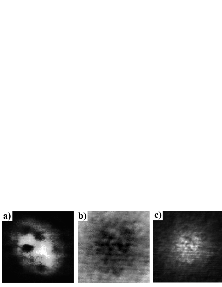
Figure 2. The sequence of nonequilibrium states observed in experiment: (a) vortex state, (b) vortex turbulence, (c) grain turbulence. The density snapshots, obtained in the time-of-flight setup, are presented. Darker spots correspond to lower density.

Figure 2 presents the sequence of experimentally realized states, observed in time-of-flight experiments with ⁸⁷Rb: a state with several vortices, vortex turbulent state, and the density configuration, typical of a granular state. Brighter colour corresponds to higher density.

Numerical simulations confirm that the grains have the sizes close to the coherence length $\xi\sim 10^{-5}$ cm and that the phase inside a grain is constant, hence the grains are really Bose-condensed coherent droplets. If the pumping by the alternating external potential is stopped, each grain survives during the lifetime $10^{-2}$ s, which is much longer than the local equilibration time of $10^{-4}$ s. That is, the fog made of these Bose-condensed grains can be treated as a metastable object, similarly to the fog made of water droplets [45]. The density inside a grain is up to $100$ times larger than that of their surrounding. It is worth stressing that the grains as well as their surrounding are formed by the same atoms. In that sense, the system should not be treated as composed of different species [46], but rather it could be interpreted as consisting of different phases [33].

During the regime of grain turbulence, the grains do not essentially change their sizes, increasing only very little. Since the transition between vortex turbulence and grain turbulence is a crossover, in the grain-turbulent state there can occur occasional vortices, although they are rare.

2.5 Wave turbulence

After the injected energy becomes comparable to the energy $E_{c}\equiv k_{B}T_{c}$, where $T_{c}$ is the Bose-Einstein condensation temperature, all condensate is destroyed, and the system represents the state of wave turbulence, or weak turbulence. For ⁸⁷Rb atoms, $T_{c}=2.76\times 10^{-7}$ K. Hence, $E_{c}=0.238\times 10^{-10}$ eV, which gives $E_{c}=27.4E_{\perp}$.

Contrary to grains, the waves in the regime of wave turbulence are small-amplitude nonuniformities, being just three times denser than their surrounding. The typical size of a wave is of order $10^{-4}$ cm, and the phase inside it is random, which implies that there are no coherent regions that would be related to Bose-Einstein condensate. In the regime of wave turbulence, the Bose condensate is getting destroyed.

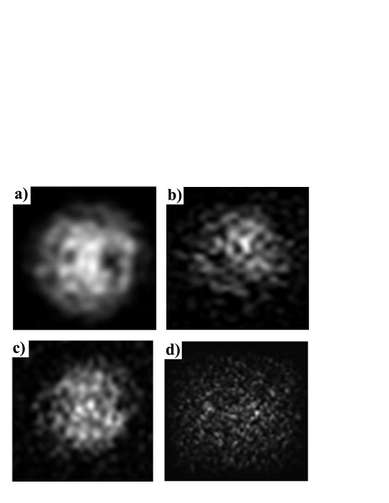
Figure 3. The sequence of nonequilibrium states realized in numerical modeling: (a) vortex state, (b) vortex turbulence, (c) grain turbulence, (d) wave turbulence. The density cross-sections are demonstrated. Brighter colour corresponds to higher density.

Because of the high energy required for creating the wave turbulence, this regime has not yet been achieved in experiments, but has been realized in numerical modeling. The whole sequence of nonequilibrium states, found numerically, is presented in Fig. 3.

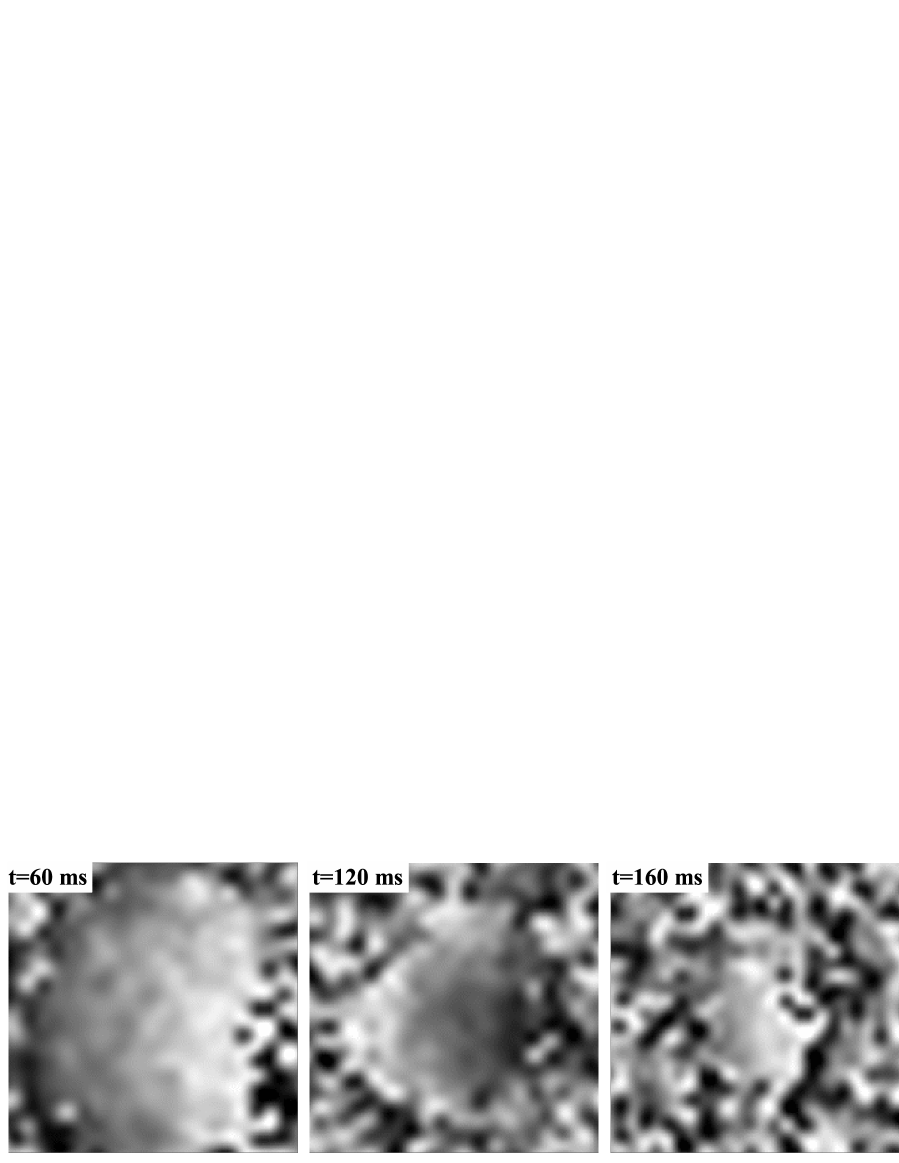
Figure 4. The sequence of snapshots of the system phase at consecutive moments of time, the phase being gradually destroyed under increasing injected energy.

Recall that the transitions between the dynamic regimes are crossovers, but not sharp phase transitions. But, as is seen from Fig. 1 for the number of vortices as a function of time, the transitions from the vortex state to vortex turbulence and from vortex turbulence to grain turbulence are rather sharp. Contrary to this, the transformation from grain turbulence to wave turbulence is rather gradual, the grains and waves coexist in a wide temporal range. The number of coherent grains diminishes with time, while the number of waves increases. The system coherence is being destroyed in a slow pace. First, coherence is destroyed at the surface of the atomic cloud. The snapshots of the phase are shown in Fig. 4. The crossover line, conditionally separating the regimes of grain turbulence and wave turbulence, can be located at the moment, when the system coherence, associated with grains, is destroyed in approximately half of the system, the incoherent region being associated with waves.

During the process of pumping, the kinetic energy of the system, $E_{kin}$, increases, as compared to the energy of atomic interactions $E_{int}$. This is illustrated in Fig. 5. In the region of weak nonequilibrium, the interaction energy is much larger than kinetic energy. The vortex state, appearing at $t_{vor}=18$ ms and ending at $t_{tur}=28$ ms, is characterized by the ratio of kinetic to interaction energy between $1.8$ and $4.2$. Vortex turbulence, arising at $t_{tur}=28$ ms and lasting till $t_{fog}=37$ ms, is described by the ratio $E_{kin}/E_{int}$ between $4.2$ and $6.7$. Under grain turbulence, existing in the interval from $t_{fog}=37$ ms to $t_{c}=120$ ms, the ratio $E_{kin}/E_{int}$ varies from $6.7$ to $74$. In the regime of wave turbulence, kinetic energy is much higher than interaction energy, so that $E_{kin}/E_{int}$ is of order $50$ to $100$.

3 Discussion

When a system, being prepared in a strongly nonequilibrium symmetric state, equilibrates on a finite time scale to a state with broken symmetry, there appear topological defects, such as vortices, protodomains, cells, or grains, strings, and monopoles. This is called the Kibble-Zurek mechanism that can be illustrated by various systems, from different kinds of condensed matter to cosmological objects [1, 2, 3, 4, 5, 47, 48]. In the particular case of nonequilibrium Bose condensation, the equilibration process starts with the nonequilibrium state of wave turbulence and ends in an equilibrium Bose-condensed state [49, 50].

We have shown that there exists the inverse Kibble-Zurek scenario, when we start with an equilibrium system with broken symmetry and, by imposing perturbations, transform it to a strongly nonequilibrium symmetric state through the sequence of states with spontaneously arising topological defects. This is demonstrated by considering a trapped Bose-Einstein condensate, perturbing which we realize a sequence of states whose order is opposite to that arising in the process of equilibration of an uncondensed system to its Bose condensed state. All intermediate states with topological defects are recovered, although in the opposite to the Kibble-Zurek mechanism order. Starting with an equilibrium Bose condensate, by increasing perturbation, we consecutively observe the creation of separate vortices, vortex turbulence, condensed cells, or grains, and wave turbulence with Bose condensate being destroyed. These are the same states that would appear in the opposite order, if an uncondensed nonequilibrium system would equilibrate to its Bose condensed equilibrium. We demonstrate the inverse Kibble-Zurek scenario both experimentally, by perturbing the Bose-Einstein condensate of trapped ⁸⁷Rb atoms, and also by accomplishing numerical simulations for the same setup as in the experiment, the experimental and numerical results being in good agreement with each other.

The summary of the realized states, depending on the amount of the injected energy, is as follows:

$E_{inj}=0$	(equilibrium state)
$0<E_{inj}<2E_{vor}$	(weak nonequilibrium)
$2E_{vor}<E_{inj}<E_{tur}$	(vortex state)
$E_{tur}<E_{inj}<E_{fog}$	(vortex turbulence)
$E_{fog}<E_{inj}<E_{c}$	(grain turbulence)
$E_{inj}>E_{c}$	(wave turbulence) .

In terms of temporal scale, the observed nonequilibrium regimes occur in the intervals

$t=0$	(equilibrium state)
$0<t<t_{vor}$	(weak nonequilibrium)
$t_{vor}<t<t_{tur}$	(vortex state)
$t_{tur}<t<t_{fog}$	(vortex turbulence)
$t_{fog}<t<t_{c}$	(grain turbulence)
$t>t_{c}$	(wave turbulence) ,

where $t_{vor}=18$ ms, $t_{tur}=28$ ms, $t_{fog}=37$ ms, and $t_{c}=120$ ms.

Introducing the relative injected energy

$$\varepsilon\equiv\frac{E_{inj}}{E_{vor}}\;,$$

normalized to the vortex energy, the sequence of the states in the inverse Kibble-Zurek scenario, we have realized, is characterized by the relations

$\varepsilon=0$	(equilibrium state)
$0<\varepsilon<2$	(weak nonequilibrium)
$2<\varepsilon<25$	(vortex state)
$25<\varepsilon<30$	(vortex turbulence)
$30<\varepsilon<100$	(grain turbulence)
$\varepsilon>100$	(wave turbulence) .

The injected energy (3), for the used oscillating perturbation potential is approximately proportional to time, after it is much longer than the period of the modulating field, $t\gg 2\pi/\omega$, which is of order $10$ ms. Thus, we have

$$\frac{E_{fog}}{E_{tur}}\sim\frac{t_{fog}}{t_{tur}}\sim 1\;,\qquad\frac{E_{c}}{E_{fog}}\sim\frac{t_{c}}{t_{fog}}\sim 3\;.$$

The different dynamic regimes are not separated by sharp boundaries, but, strictly speaking, occur continuously. That is, these dynamic transitions are crossovers, but not abrupt phase transitions, although they may happen rather noticeably. Therefore the neighboring states can occasionally display the features typical of their lower-energy member. For instance, in the regime of grain turbulence, there may happen occasional vortices. And in the regime of wave turbulence, waves coexist with grains.

Thus we have demonstrated that the Kibble-Zurek mechanism is reversible, at least for the process of Bose-Einstein condensation versus Bose condensate destruction. The demonstration of the inverse Kibble-Zurek scenario for trapped atoms opens a new direction of studying the universality of the reversibility of this mechanism, investigating whether it is reversible for other physical systems of different nature.

Acknowledgments We appreciate financial support from FAPESP and RFBR (Grant 14-02-00723). We are grateful to M. Tsubota and E.P. Yukalova for discussions.

Figure Captions

Figure 1. Number of vortices as a function of the pumping time, under fixed modulation amplitude, found in numerical simulations.

Figure 5. The ratios of interaction energy to kinetic energy of the system, $E_{int}/E_{kin}$ (thick line), and of kinetic to interaction energy, $E_{kin}/E_{int}$ (thin line), as functions of the time of pumping.

Figure 1: Number of vortices as a function of the pumping time, under fixed modulation amplitude, found in numerical simulations.

Figure 2: The sequence of nonequilibrium states observed in experiment: (a) vortex state, (b) vortex turbulence, (c) grain turbulence. The density snapshots, obtained in the time-of-flight setup, are presented. Darker spots correspond to lower density.

Figure 3: The sequence of nonequilibrium states realized in numerical modeling: (a) vortex state, (b) vortex turbulence, (c) grain turbulence, (d) wave turbulence. The density cross-sections are demonstrated. Brighter colour corresponds to higher density.

Figure 4: The sequence of snapshots of the system phase at consecutive moments of time, the phase being gradually destroyed under increasing injected energy.

Figure 5: The ratios of interaction energy to kinetic energy of the system, $E_{int}/E_{kin}$ (thick line), and of kinetic to interaction energy, $E_{kin}/E_{int}$ (thin line), as functions of the time of pumping.

References

- [1] T.W.B. Kibble, J. Phys. A 9 (1976) 1387.
- [2] T.W.B. Kibble, Phys. Rep. 67 (1980) 183.
- [3] W.H. Zurek, Nature 317 (1985) 505.
- [4] W.H. Zurek, Phys. Rep. 276 (1996) 177.
- [5] W.H. Zurek, Nature 382 (1996) 296.
- [6] K. Pyka, J. Keller, H.L. Partner, R. Nigmatullin, T. Burgermeister, D.M. Meier, K. Kuhlmann, A. Retzker, M.B. Plenio, W.H. Zurek, A. del Campo, T.E. Mehlstübler, Nature Commun. 4 (2013) 2291.
- [7] S. Ulm, J. Rossnagel, G. Jacob, C. Degünther, S.T. Dawkins, U.G. Poschinger, R. Nigmatullin, A. Retzker, M.B. Plenio, F. Schmidt-Kaler, K. Singer, Nature Commun. 4 (2013) 3290.
- [8] R. Carmi, B. Polturak, Phys. Rev. B 60 (1999) 7595.
- [9] C.Bäuerle, Y.M. Bunkov, S.N. Fisher, H. Godfrin, G.R. Pickett, Nature 382 (1996) 332.
- [10] V.M.H. Ruutu, V.B. Eltsov, A.J. Gill, T.W.B. Kibble, M. Krusius, Y.G. Makhlin, B. Plaçais, G.E. Volovik, W. Xu, Nature 382 (1996) 334.
- [11] P.C. Hendry, N.S. Lawson, R.A.M. Lee, P.V.E. McClintock, C.D.H. Williams, Nature 368 (1994) 315.
- [12] C.N. Weiler, T.W. Neely, D.R. Scherer, A.S. Bradley, M.J. Davis, B.P. Anderson, Nature 455 (2008) 948.
- [13] G. Lamporesi, S. Donadello, S. Serafini, F. Dalfovo, G. Ferrari, Nature Phys. 9 (2013) 656.
- [14] N. Navon, A.L. Gaunt, R.P. Smith, Z. Hadzibabic, Science 347 (2015) 167.
- [15] E. Levich, V. Yakhot, Phys. Rev. B 15 (1977) 243.
- [16] H.T.C. Stoof, Phys. Rev. A 45 (1992) 8398.
- [17] Y. Kagan, B.V. Svistunov, Phys. Rev. Lett. 79 (1997) 3331.
- [18] V.E. Zakharov, S.V. Nazarenko, Physica D 201 (2005) 203.
- [19] D.W. Snoke, J.P. Wolfe, Phys. Rev. B 39 (1989) 4030.
- [20] D.V. Semikoz, I.I. Tkachev, Phys. Rev. D 55 (1997) 489.
- [21] N.G. Berloff, B.V. Svistunov, Phys. Rev. A 66 (2002) 013603.
- [22] R.P. Feynman, Prog. Low Temp. Phys. 1 (1955) 17.
- [23] G.A. Williams, Phys. Rev. Lett. 82 (1999) 1201.
- [24] N.D. Antunes, L.M.A. Bettencourt, W.H. Zurek. Phys. Rev. Lett. 82 (1999) 2824.
- [25] S.K. Nemirovskii, Theor. Math. Phys. 141 (2004) 1452.
- [26] S.K. Nemirovskii, L.P. Kondaurova, J. Low Temp. Phys. 156 (2009) 182.
- [27] E.A.L. Henn, J.A. Seman, G. Roati, K.M.F. Magalhães, V.S. Bagnato, Phys. Rev. Lett. 103 (2009) 045301.
- [28] R.F. Shiozaki, G.D. Telles, V.I. Yukalov, V.S. Bagnato, Laser Phys. Lett. 8 (2011) 393.
- [29] J.A. Seman, E.A.L. Henn, R.F. Shiozaki, G. Roati, F.J. Poveda-Cuevas, K.M.F. Magalhães, V.I. Yukalov, M. Tsubota, M. Kobayashi, K. Kasamatsu, V.S. Bagnato, Laser Phys. Lett. 8 (2011) 691.
- [30] V.I. Yukalov, E.P. Yukalova, V.S. Bagnato, Phys. Rev. A 56 (1997) 4845.
- [31] J.L. Birman, R.G. Nazmitdinov, V.I. Yukalov, Phys. Rep. 526 (2013) 1.
- [32] V.S. Bagnato, V.I. Yukalov, Prog. Opt. Sci. Photon. 1 (2013) 377.
- [33] V.I. Yukalov, Laser Phys. 23 (2013) 062001.
- [34] I. Br̆ezinová, L.A. Collins, K. Ludwig, B.I. Schneider, J. Burgdörfer, Phys. Rev. A 83 (2011) 043611.
- [35] V.I. Yukalov, Phys. Lett. A 253 (1999) 173.
- [36] V. Blum, G. Lauritsch, J.A. Maruhn, P.G. Reinhard, J. Comput. Phys. 100 (1992) 364.
- [37] L.P. DeVries, AIP Conf. Proc. 160 (1987) 269.
- [38] M. Tsubota and M. Kobayashi, H. Takeushi, Phys. Rep. 522 (2013) 191.
- [39] S.K. Nemirovskii, Phys. Rep. 524 (2013) 85.
- [40] C.J. Pethick, H. Smith, Bose-Einstein Condensation in Dilute Gases, Cambridge University, Cambridge, 2008.
- [41] P.W. Courteille, V.S. Bagnato, V.I. Yukalov, Laser Phys. 11 (2001) 659.
- [42] V.I. Yukalov, E.P. Yukalova, V.S. Bagnato, Laser Phys. 12 (2002) 231.
- [43] C.J. Foster, P.B. Blakie, M.J. Davis, Phys. Rev. A 81 (2010) 023623.
- [44] V.I. Yukalov, Laser Phys. Lett. 7 (2010) 467.
- [45] V.I. Yukalov, A.N. Novikov, V.S. Bagnato, Laser Phys. Lett. 11 (2014) 095501.
- [46] M.B. Pinto, R.O. Ramos, F.F. de Souza Cruz, Phys. Rev. A 74 (2006) 033618.
- [47] A. Polkovnikov, K. Sengupta, A. Silva, and M. Vengalatore, Rev. Mod. Phys. 83 (2011) 863.
- [48] V.I. Yukalov, Laser Phys. Lett. 8 (2011) 485.
- [49] V.E. Zakharov, V.S. Lvov, G.E. Falkovich, Kolmogorov Spectra of Turbulence: Wave Turbulence, Springer, Berlin, 1992.
- [50] S. Nazarenko, Wave Turbulence, Springer, Berlin, 2011.