]Received
Gluon Propagation in Curved Space
Abstract
In quantum chromodynamics (QCD), the vacuum structures are taken to be formed by nonperturbative interactions between gluons. The contributions of gluonic interactions can be parametrized by gluon condensates and especially the dimension-2 condensate can be used to generalize the vacuum. In the generalized picture, each gauge fixed slice forms a curved surface around a hadron and other strongly interacting objects, and the propagation of a gluon has to be considered on this curved surface. The gluon propagator turns out to be massive due to the curvature of the gauge fixed surface implementing the possibility that the massless gauge bosons might provide the majority of the hadronic mass and even behave as dark matter in cosmological scales.
pacs:
11.15.Tk, 12.38.Lg, 12.90.+bI INTRODUCTION
The strong interactions are taken to be mediated by gluons and the most peculiar aspect of gluonic interactions is the nonperturbative self-interactions. These nonperturbative self-interactions generate the problem of definition of vacuum state which is the starting point of any calculation by using the properties of quantized fields such as propagators. The vacuum states for strong interactions are known to be classified according to their topological quantum numbers R1 and those classified states turn out to be mixed through instantons R2 . The condition that the vacuum state has to be stationary with respect to gauge transformations leads to the definition of vacuum R3 resulting from the undetermined angle appearing in the eigenvalue of gauge transformation. Because the number of possible values of is infinite, the gluonic vacuum states can exist in infinitely different states physically independent from each other. However, in ordinary picture, infinitely many vacuum states may generate infinitely different vacuum expectation values which lead immediately to contradictory results with experimental observations.
The solution to the problem of infinitely many vacuum states appeared as a by-product of the consideration of in-hadron condensates R4 . The vacuum condensates R5 are defined as the nonzero vacuum expectation values of normal ordered products of field operators and are usually taken to be constant with respect to space-time variables. A well-known effect of vacuum condensates is the modification of quark and gluon propagators resulting in the damping in propagation R6 . The damping arises due to background fields residing within hadronic scales and therefore the vacuum condensates have to be considered only within the scale of hadronic size. In this way the idea of in-hadron condensates has been suggested and various examples are discussed with the introduction of maximum wavelength of quarks and gluons confined in hadrons. Although the in-hadron condensate idea resolved many problems, there existed intrinsic restrictions concerning the boundary values of condensates if the condensate values are taken to be constant inside hadrons. The only breakthrough to this restriction is to assume the variation of condensate values resulting in the new picture of QCD vacuum R7 composed by union of different gauge fixed slices.
The new picture of QCD vacuum generalizes the picture of vacuum with coordinate dependent values R8 . These coordinate dependences can be parametrized by the values of dimension-2 condensates R9 and for a given value of dimension-2 condensate the set of points constitute a curved surface around a hadron. Each surface represents one gauge fixed slice corresponding to one vacuum and the infinitely many vacua can be drawn as different surfaces around a hadron. Of course this picture can be applied to the more complicated situations such as multi-quark states or nuclei and even to the extreme case of quark-gluon plasma. In fact, the generalization of vacuum with coordinate dependences has been suggested as one possible scenario R10 to explain the strong CP problem in hot quark-gluon matter. Recent experiments at RHIC and LHC confirmed the P-odd charge separation effects R11 and the generalized vacuum can be taken as the state where the gluonic behaviors have to be analyzed.
Calculational method for the structures of gauge fixed slices has been developed by considering topological spaces of gluonic domains R12 which can be classified according to the numbers of quarks and antiquarks inside each gluonic domain. For a given topological space, the changes of gluonic domains are induced by quark pair creation or annihilation and the probability amplitude to have a quark pair is taken to be proportional to the value of dimension-2 condensate at that point R13 . When these considerations are combined with the amplitude defined by nonlocal condensate between two quarks, we can deduce functional form of the variation of dimension-2 condensate. The surface formed by the points with the same value of dimension-2 condensate constitutes one gauge fixed slice and we can draw infinitely many slices by changing the value of dimension-2 condensate. Thus the QCD vacuum around a hadron or other structures such as multi-quark states and nuclei can be pictured by the union of each gauge slice formed by given value of dimension-2 condensate.
For a given QCD vacuum, we can try to deduce the Feynman rules and the most important quantity is the gluon propagator. In order to deduce the form of gluon propagator we have to fix the gauge and the quantization procedure has to be carried out on this gauge fixed slice. But now the gauge fixed slices turn out to be curved surfaces and the quantization of gluons has to be considered on the curved space. The first effects of curved space are the changes of derivatives from the ordinary ones into the covariant ones R14 . These changes give rise to additional terms related to the curvature of the space. In the simplest case the additional term can be interpreted as carrying out the role of mass term in gluon propagator, and thus there appears the possibility that the masslessness of gluons as gauge bosons can be changed naturally into the massiveness of hadrons or other strongly interacting objects. For cosmological scales these considerations may lead to one possible candidate for dark matter R15 .
In Sec. II, we review the procedure of generalization of vacuum, and in Sec. III, we show the structures of gauge fixed slices. In Sec. IV, we deduce the form of gluon propagator in curved space, and in Sec. V, we suggest gluons as dark matter candidate. The final section is devoted to summary and discussions.
II GENERALIZED VACUUM
For atomic structure, the composing elements are nucleus and electrons and these elements have definite masses with nonrelativistic movements. The vacuum state for an atom is taken to be a state in which nothing exists. From this vacuum state we can count the number of electrons and an atom is formed with these definite number of electrons and nucleus. However, as we approach the nucleus it becomes impossible to count the number of electrons because electron-positron pairs are continuously created and annihilated as the energy of the probing particle goes beyond 1 MeV. Then the vacuum state for a nucleus cannot be a state of nothing. It is a state of somethings that are created and annihilated continuously. In order to describe physical quantities systematically we need to arrange the creation and annihilation of particles in a definite manner and the resulting method is known as normal ordering. In quantum field theories, the method of normal ordering is fully exploited to define physical quantities.
The situation changes once again when we consider nonperturbative self-interactions of gluons. The normal ordering method is useful only when we can count the number of particles in a given state. But due to the nonperturbative self-interactions the number of gluons in a state cannot be counted appropriately. Therefore vacuum expectation values of normal ordered field operators do not vanish for gluonic states and these are parametrized as vacuum condensates. The original idea of condensate was applied only to gauge invariant forms of field operators and the field operators were classified according to their dimensions. However, after three loop calculations had been carried out R16 , there appeared the necessity of introducing dimension-2 condensate which depended on the choice of gauge. If something is dependent on the choice of gauge, it can be used to fix the gauge. Since the quantization procedure of gluons has to be carried out with gauge fixing, the slice with given value of dimension-2 condensate can be the appropriate place where the quantization of gluons could be performed. The collections of these gauge slices are intimately related to the generalization of vacuum.
The definition of vacuum starts from the instanton solution to minimize the Yang-Mills action satisfying
| (1) |
To induce the form of satisfying these equations, we consider the transformation properties of at long distances and get
| (2) |
where represents the matrix element of the group of gauge transformations. In Euclidean space with imaginary time, the set of points at infinity in four dimensional space forms a large sphere and the above relation generates mappings between the points on and the group elements . These mappings classify the gauge fields into infinitely many independent components. For a group element , the gauge field for a vacuum is given by
| (3) |
Representing the mapping corresponding to times repetition of as
| (4) |
the gauge field given by
| (5) |
constitutes another vacuum state locally. When we write the wave functional for this vacuum state as , the other vacuum state at can exist and these states can be mixed through tunnelling. Then the true vacuum state can be written as
| (6) |
and the coefficients can be determined from the condition that has to be stationary with respect to gauge transformations. The final result is
| (7) |
and this state is called the vacuum.
Now the parameter remains as a free parameter. For two different and the transition amplitude becomes
| (8) |
The exponential factor in front of the functional integral represents the change of vacuum winding number and this factor can be inserted into the functional integral by changing the Lagrangian density as
| (9) |
in Minkowski space. The second term breaks the and invariances and these effects have been checked by the measurement of neutron electric dipole moment resulting in the limit . However, in recent experiments at RHIC and LHC, local P-odd effects are observed implementing the possibility that topological fluctuations exist in hot quark-gluon matter. Then there exist definite differences between the gluonic states of a neutron and hot quark-gluon matter. Because the differences are generated by instantons, we need to analyze the relationships between the instanton contributions and the structures of QCD vacuum. These relationships have been checked by considering the correlation function on a lattice in one approach, and by using the instanton shape recognition procedure on the lattice in another approach. From the comparison of two-point correlation function with the lattice gluon propagator, correction to gluon propagator has been confirmed indicating the existence of dimension-2 condensate R17 . By using instanton shape recognition procedure R18 we can also confirm the presence of dimension-2 condensate and the expected values are well explained in an instanton-gas or an instanton-liquid picture.
For topologically non-trivial vacuum states, the strong interaction Lagrangian is given by
| (10) |
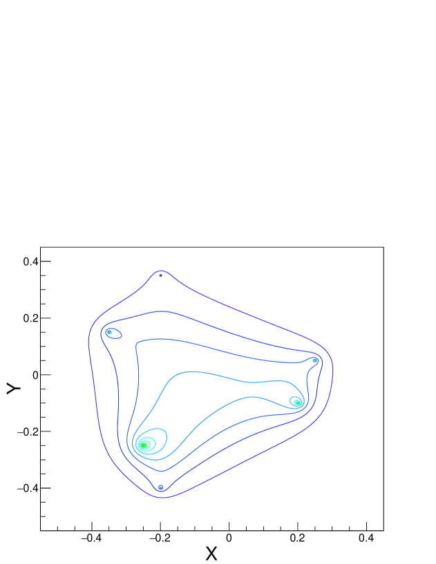
The -term characterizes the vacuum state and the observations of parity-odd domains localized in space and time strongly support the spacetime dependence of as . In case of varying values, the vacuum domains can be classified by the conditions with fixed values of . The classified points constitute surfaces and according to the movements of quarks the forms of surfaces will change. For example, the points with fixed ’s for 6 quark configuration can be drawn as in Fig. 1 R19 . This configuration can be made in the scattering processes of proton-proton collisions. Since the different surfaces correspond to different values of , we have to consider the strong interaction vacuum as formed by the union of different slices in case of spacetime dependent . For a given slice, the instanton contribution can be estimated by the value of dimension-2 condensate . Then we can assign another value of to another slice. These configurations can be represented as
| (11) |
with fixed for each slice. For different slices we can write
| (12) |
and the spacetime dependence of is transferred into that of . The whole QCD vacuum is now composed of these slices establishing the generalized vacuum R20 .
III STRUCTURE OF GAUGE FIXED SLICES
In general relativity, gauge invariance stems from the independence of the field equations on the choice of coordinate system. The Einstein field equations depend only on metric tensor and energy-momentum of the system, and therefore the choice of a coordinate system does not affect the equations of motion. However, in order to solve the equations of motion it is quite important to choose the coordinate system and this choice of particular system corresponds to the fixing of particular gauge R21 . For quantum field theories, the main variables are changed into the field variables at each space-time point, and since the field variables generally include internal degrees of freedom the gauge fixing condition becomes functional relation specifying the surface on which each gauge orbit has unique position. The gauge orbit is obtained by connecting the field variables that can be related by gauge transformations. Thus the determination of functional relation for gauge fixing is a dual process with respect to the following up the gauge orbit R22 .
For the space of gluonic field , the condition for gauge fixing can be written as
| (13) |
Traditionally the functional form of had been taken to be linear in because of simplicity and the corresponding surface is taken to be a plane in the field space. However, now we have the generalized vacuum defined by the union of gauge slices given in Eq.(12) where the functional form is quadratic. The quadratic form originates from the existence of dimension-2 condensate due to the nonperturbative self-interactions of gluons. These gluonic self-interactions induce that the gluonic states cannot be classified according to the number of gluons and the unique possibility to define the gluonic state is to consider the state of infinite number of gluons. Let this state be represented by and then we have
| (14) |
because the gluon number is not changed by one creation or by one annihilation. We get the covariant relation
| (15) |
with inner producting each side. This condition is equivalent to the gauge slice condition in Eq.(12) if we take the state as one vacuum state. For different values we have independent vacuum states represented by different values of dimension-2 condensate. In ordinary flat space, these vacuum states might be overlapped, however, because the vacuum condensates have to be considered only around hadronic structure as indicated by in-hadron condensates, the QCD vacuum is taken to be the union of curved slices fixed by the value of dimension-2 condensate.
In order to figure out the structure of gauge fixed slices, we need to classify the gluonic domains formed by slices with given values of dimension-2 condensate. Because the gluonic domains are made around quarks and antiquarks which behave as sources and sinks of the gluons, we can classify the domains by the numbers of quarks and antiquarks in each domain. If we represent the gluonic domain around quarks and antiquarks as , then meson domain is represented by , and baryon domain corresponds to . In this representation we can include arbitrary number of quarks and antiquarks such as , however, since the final states of strong interactions are observed as hadrons we need to categorize the gluonic domains with definite rules of combinations. Two gluonic domains are united when one quark-antiquark pair annihilates and conversely one gluonic domain can be divided into two domains by one quark-antiquark pair creation. Therefore the union and the intersection operations can be defined into the sets of gluonic domains, which can be formulated as follows R23 :
-
Gluonic domains are open sets.
-
The union of gluonic domains is a glunoic domain.
-
The intersection between a connected gluonic domain and disconnected gluonic domains is the reverse operation of the union.
These are just the conditions needed to construct the topological spaces of gluonic domains. The constructed topological space encompassing baryons and antibaryons can be represented as
| (16) |
For the constructed topological spaces, we may introduce a systematic measure to deduce the forms of the gauge fixed slices defined by the values of dimension-2 condensate. The measure is related to the nature of QCD vacuum and so it has to be represented by quantities characterizing the vacuum. Because the characteristics of vacuum states have been expressed as various condensates, it is plausible to compare two fundamental condensates to deduce the form of gauge fixed slice. The two fundamental condensates can be chosen as the quark condensate and the dimension-2 gluon condensate. The nonlocal quark condensate is defined by R24
| (17) |
where represents the connection through the gluonic domain. In the gluonic domain, the gluonic effects are parametrized by the value of and this value changes from point to point. The comparison with quark condensate can be made possible by assuming
| (18) |
where the final result can be expressed as products of two ’s. To derive the functional form of we consider a measure . In general, we can assume that the value of decreases as the distance between the quarks increases. This assumption can be stated as
| (19) |
Another condition can be written down by comparing both sides of Eq.(18) resulting in
| (20) |
Then these two conditions lead to the solution
| (21) |
where is an appropriate parameter and is a normalization constant. When we try to represent the measure as a metric function, we may use the distance function
| (22) |
with and representing the positions of the quark pair. We need to sum over the contributions from different values of and the full amplitude becomes
| (23) |
The weight factor has been introduced to account for possible different contributions from different ’s, and the variable is
| (24) |
with being a scale parameter. For the case of equal weight and for , we get
| (25) |
Perturbative local effects can be included by substituting for , and then becomes
| (26) |
Introducing the notation
| (27) |
we can write the value of at the point as
| (28) |
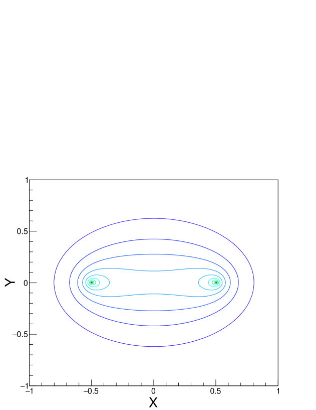
for the case of a 6-quark domain and several slices are shown in Fig. 1. For a meson domain , curved slices are shown in Fig. 2.
IV GLUON PROPAGATOR ON CURVED GAUGE SLICE
Before we discuss the gluon propagation in curved space, it is valuable to summarize the changes of ordinary gluon propagator when the dimension-2 condensate exists. For simplicity we assume that the space is flat and the value of is taken to be a constant. Because the condensate value is taken to be constant, we may decompose the gluon field as
| (29) |
where contributes to the condensate as the zero-momentum mode. Then, the effective Lagrangian density for gluons can be written as R25
| (30) |
with
| (31) |
The gluon mass is defined by the condensate value
| (32) |
and the existence of mass term indicates that the polarization tensor for a gluon has the contribution
| (33) |
If we define the scalar function by
| (34) |
then can be written as
| (35) |
The first term represents the mass effects originating from the vacuum condensate corresponding to the Schwinger mechanism, and the second term appears as the next corrections. The form of is determined by the relation
| (36) |
where
| (37) |
with
| (38) |
By putting the condition in Eq.(29) and using the relation in Eq.(32), we obtain
| (39) |
and then we get
| (40) |
With these results we can write the form of transverse gluon propagator as
| (41) |
where we can see that there exists no pole and so the gluons cannot propagate freely reaching far away from the source. This damping of gluon propagator originates from the constant dimension-2 condensate generating dynamical mass of gluon. Phenomenologically the dynamical gluon mass is determined to be about MeV R26 , however, these values are too large to be considered as the value of just one gluon because there exist so many gluons in a hadron. Moreover, the gluonic structure of hadron is not uniform as assumed in Eq.(32), so that we need to quantize the gluonic field on the curved gauge slices as shown in Fig. 1 and in Fig. 2.
The gauge slices are defined by the Eq.(15) with different values and they turn out to be curved surfaces around quarks and antiquarks forming hadronic structure. In order to account for the curvature we need to replace the ordinary derivative by the covariant derivative. The covariant derivative is defined as
| (42) |
where represents the affine connection which relates the ordinary coordinates to the freely falling coordinates. When , the difference between two covariant derivatives is given by
| (43) |
which implies that covariant curl is the same as ordinary curl and there appears no curvature effect in first order derivatives. However, the Lagrangian which is used in the derivation of the gluon propagator contains the second order derivatives and the difference between two second order derivatives becomes R27
| (44) |
where the Riemann-Christoffel curvature tensor is defined as
| (45) |
The Ricci tensor is given by
| (46) |
and the curvature scalar is defined as .
Now the free Lagrangian for gluon propagator in curved space can be written as
| (47) |
In order to carry out the functional integration we have to arrange the differential operators into the form
| (48) |
where the covariant differential operators do not commute as in Eq.(44). To compare with ordinary gluon propagator in flat space we rearrange the differential operators and get
| (49) |
with additional Ricci tensor . The gluon propagator is obtained as the inverse matrix of the tensor that appears between the two gluonic fields. In flat space, the differential operators can be replaced by momentum variables and the inverse matrix can be calculated easily. However, in curved space, the appearance of Ricci tensor makes it non-trivial to calculate the inverse matrix and we need to introduce additional assumptions to deduce the form of gluon propagator. The simplest case is that of flat space in which the Ricci tensor vanishes and we can get the ordinary form of gluon propagator. The next case is that of maximally symmetric space R28 where we can put
| (50) |
with appropriate parameter . This parameter is definitely related to the curvature scalar of the space and is obtained by considering free propagation of massless gluon as a gauge boson. Then the Lagrangian becomes
| (51) |
and the gluon propagator can be obtained as
| (52) |
which is just the propagator form of a particle with momentum and mass .
In the usual process of dynamical mass generation of gluon propagator, the polarization tensors are calculated by estimating various loop contributions with appropriate renormalization constants. Therefore the generated mass always has some uncertainty related to the renormalization process and the loop expansions turn out to be meaningless for nonperturbative gluonic interactions. Moreover the determined mass is too large to be considered as a correction to massless gluon. Instead of these difficulties, it is quite natural to get the mass effects of gluons from the curvature of gauge fixed slices.
V GLUONS AS DARK MATTER
The curved gauge slices can be drawn not only for hadrons such as mesons and baryons but also for any strongly interacting systems of quarks and gluons such as multiquark states and nuclei and even for the system of quark-gluon plasma. Because gluons are taken to be propagating along these gauge fixed slices, the curvature effects are essential in estimating the gluonic contributions to strongly interacting systems. For perturbative approximations, gluon propagators are assumed to be in the same form as that of photons except for color factors, and therefore the main features in asymptotically free region resembles those of Abelian gauge theory R29 . But in the infrared region, that is, in the confining region, nonperturbative effects play important roles in changing the vacuum states with nonvanishing condensate values. These changed vacuum states can be classified according to the configuration of the source quarks.
For stable hadrons, the configurations of quarks are very simple. In a meson, only one quark-antiquark pair exists and we can easily draw the gauge slices as in Fig. 2. However, when we want to probe the internal structure of the meson, the main scattering processes are related with the quarks and the asymptotically free gluons near the quarks leaving aside the whole bunch of gluons described as gauge slices. If the probing particle has the enough energy to approach the asymptotically free region, it can create quark-antiquark pairs and the created quarks and antiquarks change the structure of gauge slices and form the final states with new gauge slices. Because the final states are counted by hadrons instead of quarks and gluons, the nonperturbative gluons described as gauge slices behave just like the dark matter. They were not probed but contributed to the total mass of the final states.
In a baryon, three quarks have been introduced to account for the quantum numbers but their masses could not be determined in a unique way. The simplest way to determine the quark mass is to divide the total mass of a baryon by 3 and the determined mass is named as constituent quark mass R30 . Although the lowest baryon states, the proton and the neutron, have nearly the same mass, the other excited baryon states have quite different masses and therefore the value of constituent quark mass has to be different from baryon to baryon. These difficulties have lead to the idea of dynamical quark mass R31 including the effects of gluonic contributions, however, in this case also, the probed physical mass is assigned to the quark leaving the gluons as dark matter. This situation is not changed in scattering processes. In scattering processes, baryons are treated as composed of partons which carry fractional momentum of the baryon and the first approximations were made in such a way that the quarks were taken to be the partons without considering the roles of gluons. These approximations resulted in various forms of quark distribution functions R32 but could not correspond to the experimental data. The corrections to the first approximations had been made in the direction of introducing sea quarks and there appeared various models with different forms of valence quark and sea quark distribution functions R33 . Because the probing particles for the internal structures of baryons were leptons such as electrons or neutrinos, the main processes occurred through the exchange of photons or weak gauge bosons. Since the gluons did not interact directly with these gauge bosons, it was natural to introduce sea quarks instead of gluons to account for the final states. However, the total momentum carried by charged partons turned out to be only one half of the total momentum of the probed baryon. The neutral partons had to be introduced playing the role of dark matter.
The hadronic masses are basically measured by the trajectories in magnetic fields and then compared with other scattering data. The trajectories in magnetic fields are determined by the charge and the momentum of the hadron. The charge of a hadron is taken to be the sum of charges carried by valence quarks, and the momentum of the hadron is measured by the velocity of the center of mass of the hadron and the total rest mass of the hadron. But the total rest mass of a hadron is not given by the sum of rest masses of the valence quarks, and in fact, consists mostly of the intrinsically massless gluons moving around. In order to deduce the rest masses of valence quarks, we need to get rid of strong interactions and by considering electromagnetic and weak interactions we can get the values of 2.3 MeV for up quark and 4.8 MeV for down quark R34 . If we sum up these values, we have 9.4 MeV for a proton and 11.9 MeV for a neutron. These values are just of the total masses of proton and neutron. Then from the viewpoint of measurement more than of nucleon masses are dark matter which is definitely composed of gluons.
To establish the standpoint of gluons as dark matter, we need to check whether they can have survived from the Big Bang and can exist in galactic space in a nonbaryonic state. It is helpful to use the arguments of maximum wavelength of confined gluons applied to induce the idea of in-hadron condensates. It has been suggested that gluons confined in a strongly interacting system have a maximum wavelength of the order of the confinement scale R35 because they are confined within that system. Thus gluons confined in a hadron have the maximum wavelength
| (53) |
and those confined in a nucleus of diameter of 10 fm have
| (54) |
During the period of big-bang nucleosynthesis only light nuclei such as , , , and have been formed, and so the maximum wavelength of the gluons confined in such light elements can be estimated as
| (55) |
This implies that of the gluons created at the Big Bang only those with energies greater than 100 MeV could be captured inside baryons or light nuclei. Therefore the gluons with smaller energies had to be left as sterile gluons if there existed no larger structure formed by strong interactions. The heavier nuclei had been formed later in stars and in supernova explosions and the gluons with energies between 20 MeV and 100 MeV could be captured in those elements. Then how about the gluons with energies less than 20 MeV? Are there any larger structures than the heavy nuclei interacting strongly through exchanges of low energy gluons?
One possible candidate to accommodate the long wavelength gluons is the neutron star. Neutron stars are known to be formed by gravitational collapse after supernova explosions and the average density is approximately equal to the density of nucleons. This means that the neutrons inside neutron star cannot exist as independent neutrons but have to be in the form of overlapped configurations. Thus the outer part of a neutron star is taken to be in the state of solids or liquids composed of neutrons and the inner part in the state of quark-gluon plasma R36 . In the quark-gluon plasma region, the average distance between quarks is smaller than that between quarks in neutrons. Therefore the value of in Eq.(15) for the dimension-2 condensate is expected to be larger in the inner part than in the outer part of the neutron star. Because the neutron star is in the form of sphere, the gauge slices defined by Eq.(15) have to be spheres and the value is expected to be decreasing from the center of the neutron star. In order to check out the decreasing pattern of the value of dimension-2 condensate, we need to review the change of patterns for various configurations of quarks.
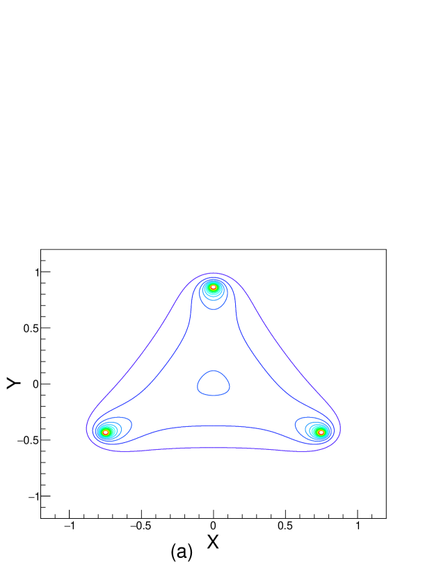
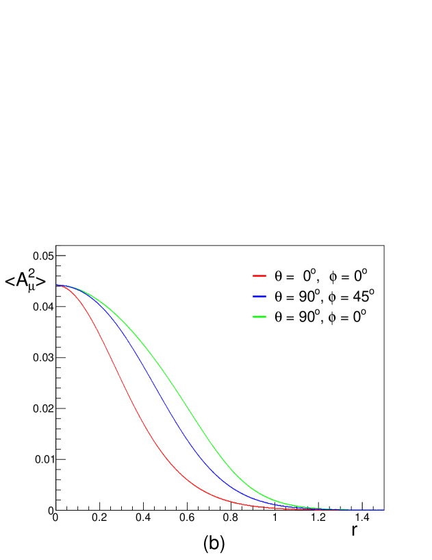
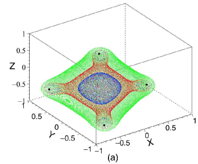
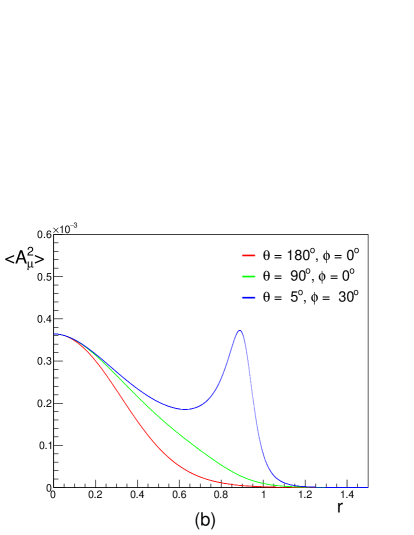
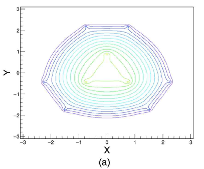
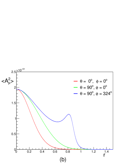
The first example to check the variance of dimension-2 condensate is the baryon. If we assume that the three quarks are located at the vertices of an equilateral triangle, we can draw the equi- surfaces as in Fig. 3(a). In Fig. 3(b), the variations of values along the axes through the center of the triangle are shown as a function of the distance from the center. The next example is a tetraquark state which can be a candidate for some particles R37 discovered in the search of excited states. A typical tetraquark configuration is drawn in Fig. 4(a) and the variations of dimension-2 condensate are shown in Fig. 4(b).
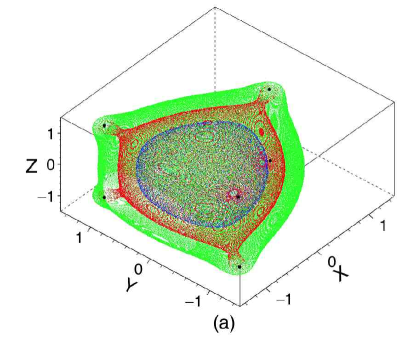
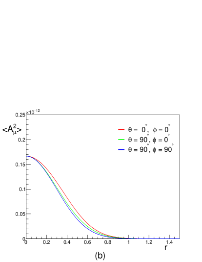
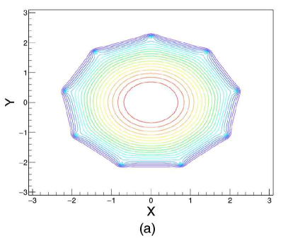
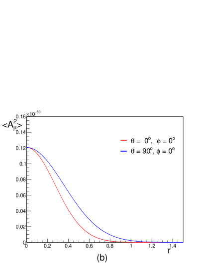
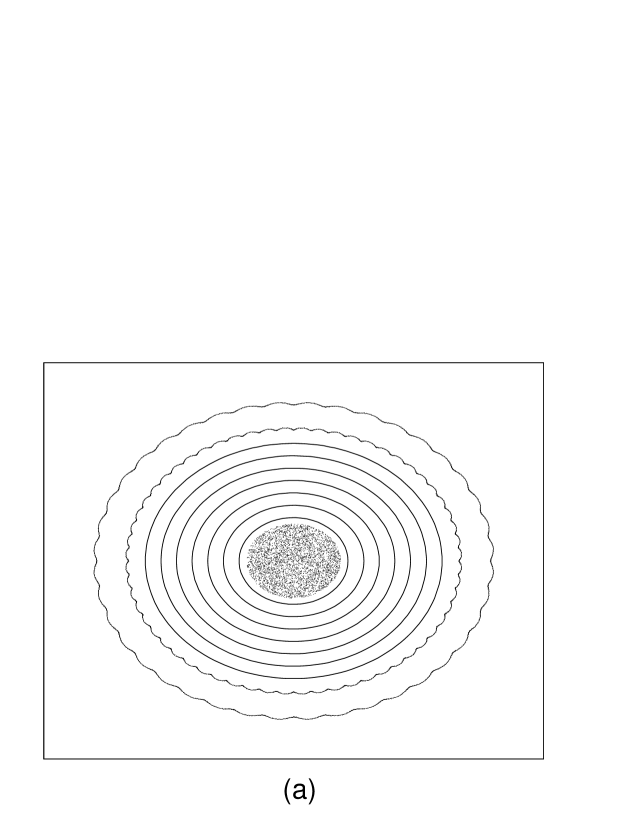
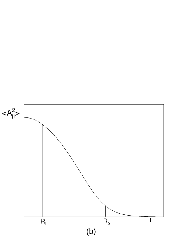
Similarly we can draw the configuration of a deuteron as in Fig. 5(a) and the condensate values are shown in Fig. 5(b). The six quarks are taken to be at the corners of a trigonal prism and the condensate values are along the 3 lines. The case of can be drawn as in Fig. 6. In Fig. 6(a), the nine quarks are at the corners of three triangles, and the condensate values are shown in Fig. 6(b). In Fig. 7, another case with the nine quarks on a circle is shown. We can find that the condensate values have maximum value at the center except for the positions of quarks and decay exponentially just outside of the quark locations. The same situation is expected to be valid for the case of quark locations in the shape of spherical shell. By combining spherical shells, we can obtain the case of sphere shape quark locations. This case is approximately in the same situation as that of a neutron star, but the neutron star contains the region of quark-gluon plasma. For the quarks in the quark-gluon plasma region, we cannot apply our nonperturbative formalism in a naive manner but their contributions to long range confining region can be induced from the above simple examples. It is expected that in the quark-gluon plasma region the values become saturated due to the perturbative interactions but the quark contributions to the values in the outer part of the neutron star could be increased. This situation is shown in Fig. 8. The radius for quark-gluon plasma region is represented by and the radius of the whole neutron star is designated as . There exist no quarks outside of and because the value extends over the space where no baryonic nor nuclear structures exist, it is possible for low energy gluons to propagate along the macroscopic spherical surfaces outside of neutron star. These gluons are not observed by photons or by neutrinos and therefore can be good candidates for dark matter.
The gluons propagating in free space may have originated from the Big Bang. As the universe expands, the energies of gluons decrease below the value of 20 MeV and then they cannot be captured in baryons or nuclei. However, they can interact with each other and form condensate structures around neutron stars and even out to the scale of a galaxy. If the sterile gluons left over after the big-bang nucleosynthesis existed uniformly over the universe, they could exist in inter-galactic regions. But somehow if they were gathering around galaxies, it is possible for them to move from inter-galactic regions to intra-galactic regions. The large scale condensate structures could be formed as nearly spherical shapes centered at each centers of mass of galaxies. Since they propagate along the spherical gauge slices, the mass effects defined by Eq.(50) could be related to the curvature scalar and we get the radius dependences as
| (56) |
These dependences are consistent with the variation of the dark matter density in a galaxy R38 . For a crude estimation of dark matter density, let’s assume that the average energy of gluons propagating in intra-galactic region is approximately 1 MeV fairly below the binding energy of deuteron 2.2 MeV. If the average number of gluons per unit volume is assumed to be the same as that of Big Bang photons 411 R39 , we have
| (57) |
which is just number obtained for the dark matter density in our galaxy.
VI DISCUSSIONS
In this paper, we reviewed the idea of generalized vacuum and showed various structures of gauge fixed slices defined by the values of dimension-2 condensates. Because the gluons have to be quantized on these gauge slices, it is essential to account for the curved structures of gauge slices. The ordinary derivatives have to be replaced by covariant ones and then from the second order form of the Lagrangian density we get the curvature dependence of the gluon propagator. The curvature dependences can be interpreted as mass effects for the case of maximum symmetry and these mass effects might be the newly found roles of gluons in hadrons and in any strongly interacting systems as dark matter.
Gluonic contributions to hadronic masses are usually parametrized as constituent quark masses which are very large compared with the current quark masses determined by electromagnetically or weakly interacting probes. The differences can be taken as dark matter in the same sense of defining the dark matter of a galaxy by the difference between measured and observed masses of a galaxy. As for the large scale confinement we can consider neutron stars as the centers for the large scale structures of gauge slices and the structures can be extended even to the whole scale of a galaxy. In general, at the center of a galaxy we expect the existence of supermassive black hole and that black hole may serve as the center for the galaxial structure of gauge slices. Since the curvature scalar decreases for the outer sphere from the center, the mass density of dark matter can be explained systematically from the large scale structure of gluon gauge slices.
Of course, there are many issues to be resolved with more detailed models. First of all, the calculation of gluon propagator with more general form of Ricci tensor is necessary. This issue is closely related to the interpretation of curvature in terms of the gluonic properties such as mass or other quantum numbers. In this connection, the argument of gluon splitting R40 could be exploited because we need to separate parallel and transverse spin components to follow up the changes along the curved gauge slices. The determination of energy spectra of sterile gluons is another issue and the coupling strength of very low energy gluons R41 could affect the final shape of cosmological dark matter distributions.
In hadronic scales, the calculations of hadronic masses with appropriate consideration of gluonic effects are important issues. Traditionally an appropriate form of confining potential is assumed between quarks and the spin-dependent forces R42 are derived by one gluon exchange diagrams in flat space. There exist some divergence problems originating from masslessness of the exchanged gluon and we need to resolve the problems with new propagator. From the distribution of gauge slices it is also possible to deduce the form of vacuum distribution functions which are used to define nonperturbative quark propagator R43 .
ACKNOWLEDGMENTS
This work was supported by research funds of Chonbuk National University in 2014.
References
- (1) A. A. Belavin et al., Phys. Lett. B 59, 85 (1975).
- (2) G. ’t Hooft, Phys. Rev. Lett. 37, 8 (1976); R. Jackiw and C. Rebbi, Phys. Rev. Lett. 37, 172 (1976).
- (3) C. G. Callan, Jr., R. F. Dashen and D. J. Gross, Phys. Lett. B 63, 334 (1976).
- (4) S. J. Brodsky and R. Shrock, Phys. Lett. B 666, 95 (2008).
- (5) M. A. Shifman, A. I. Vainshtein and V. I. Zakharov, Nucl. Phys. B 147, 385 (1979); ibid. 147, 448 (1979); ibid. 147, 519 (1979).
- (6) X. Li and C. M. Shakin, Phys. Rev. D 70, 114011 (2004); ibid. D 71, 074007 (2005).
- (7) E. J. Kim and J. B. Choi, J. Korean Phys. Soc. 61, 1215 (2012).
- (8) D. E. Kharzeev, Nucl. Phys. A 830, 543c (2009).
- (9) F. V. Gubarev, L. Stodolsky and V. I. Zakharov, Phys. Rev. Lett. 86, 2220 (2001).
- (10) D. Kharzeev, R. D. Pisarski, and M. H. G. Tytgat, Phys. Rev. Lett. 81, 512 (1998).
- (11) B. I. Abelev et al. (STAR Collaboration), Phys. Rev. C 81, 054908 (2010); B. Abelev et al. (ALICE Collaboration), Phys. Rev. Lett. 110, 012301 (2013).
- (12) E. J. Kim, J. B. Choi and M. Q. Whang, J. Korean Phys. Soc. 56, 1787 (2010).
- (13) E. J. Kim et al., J. Korean Phys. Soc. 58, L1053 (2011).
- (14) S. Weinberg, Gravitation and Cosmology (John Wiley & Sons, New York, 1972), p103.
- (15) Paticle Data Group, Chinese Phys. C 38, 090001 (2014), p353.
- (16) Ph. Boucaud et al., Phys. Rev. D 63, 114003 (2001).
- (17) Ph. Boucaud et al., Phys. Lett. B 493, 315 (2000).
- (18) Ph. Boucaud et al., Phys. Rev. D 66, 034504 (2002).
- (19) E. J. Kim and J. B. Choi, J. Korean Phys. Soc. 64, L495 (2014).
- (20) E. M. Kim et al., J. Korean Phys. Soc. 64, 1272 (2014).
- (21) Ref. R14 , p254.
- (22) B. DeWitt, 50 Years of Yang-Mills Theory (World Scientific, edited by G. ’t Hooft, 2005), p15.
- (23) J. B. Choi and S. U. Park, J. Korean Phys. Soc. 24, 263 (1991).
- (24) S. V. Mikhailov and A. V. Radyushkin, Phys. Rev. D 45, 1754 (1992).
- (25) X. Li and C. M. Shakin, Phys. Rev. D 71, 074007 (2005).
- (26) See the parameters in Ref. R25 .
- (27) Ref. R21 , p140.
- (28) Ref. R21 , p383.
- (29) K. I. Kondo and T. Shinohara, Phys. Lett. B 491, 263 (2000).
- (30) J. J. J. Kokkedee, The Quark Model (W. A. Benjamin, New York, 1969), p15.
- (31) M. Takizawa, K. Kubodera and F. Myhrer, Phys. Lett. B 261, 221 (1991).
- (32) J. Kuti and V. F. Weisskopf, Phys. Rev. D 4, 3418 (1971).
- (33) S. F. Tuan et al., Phys. Rev. D 10, 2124 (1974).
- (34) Ref. R15 , p732.
- (35) S. J. Brodsky et al., arXiv:1005.4610 [nucl-th].
- (36) F. Weber et al., Neutron Stars and Pulsars (Cambridge Univ. Press, edited by J. van Leeuwen, 2013), p61.
- (37) Ref. R15 , p78.
- (38) See Ref. R15 .
- (39) Ref. R15 , p369.
- (40) A. J. Niemi and N. R. Walet, Phys. Rev. D 72, 054007 (2005).
- (41) C. S. Fischer, A. Maas and J. M. Pawlowski, arXiv:0810.1987 [hep-ph].
- (42) E. Eichten and F. Feinberg, Phys. Rev. D 23, 2724 (1981); D. Gromes, Phys. Rep. 200, 186 (1991).
- (43) See, for example, O. Andreev, Phys. Rev. D 82, 086012 (2010).