Improving the lifetime of the NV center ensemble coupled with a superconducting flux qubit by applying magnetic fields

Abstract

One of the promising systems to realize quantum computation is a hybrid system where a superconducting flux qubit plays a role of a quantum processor and the NV center ensemble is used as a quantum memory. We have theoretically and experimentally studied the effect of magnetic fields on this hybrid system, and found that the lifetime of the vacuum Rabi oscillation is improved by applying a few mT magnetic field to the NV center ensemble. Here, we construct a theoretical model to reproduce the vacuum Rabi oscillations with/without magnetic fields applied to the NV centers, and we determine the reason why magnetic fields can affect the coherent properties of the NV center ensemble. From our theoretical analysis, we quantitatively show that the magnetic fields actually suppress the inhomogeneous broadening from the strain in the NV^- centers.

Hybridization is a promising approach for quantum computation Wallquist and et al (2009); Xiang and et al (2013). Each system has characteristic with its own advantages and disadvantages. To couple different systems, we hope to pick up the advantage which each system has. One of the candidates for such hybrid systems is a superconducting circuit such as a superconducting flux qubit (FQ) and an electron spin ensemble such as nitrogen-vacancy (NV^-) centers Imamoğlu (2009); Wesenberg and et al (2009); Schuster and et al (2010); Wu and et al (2010); Kubo and et al (2010); Amsüss and et al (2011); Kubo and et al (2011); Zhu et al. (2011); Kubo and et al (2012a, b); Marcos and et al (2010); Twamley and Barrett (2010); Matsuzaki and Nakano (2012); Saito et al. (2013); Julsgaard and et al (2013); Diniz and et al (2011); Zhu et al. (2014); Sandner et al. (2012), as described in the Fig. 1. High controllability of superconducting FQs has already been achieved with existing technology Clarke and Wilhelm (2007). Reliable gate operations have been already demonstrated Bylander and et al (2011). Quantum non-demolition measurements can be performed by Josephson bifurcation amplifier Clarke and Wilhelm (2007). However, despite significant effort, the coherence time of the FQ is of the order of $10$ $\mu$s Bylander and et al (2011); Stern et al. (2014). On the other hand, the NV^- center has a long coherence time Balasubramanian and et al (2009); Takahashi et al. (2008); Mizuochi et al. (2009); Kurucz et al. (2011); Ishikawa et al. (2012); Maurer et al. (2012); Bar-Gill et al. (2013). With dynamical decoupling, the coherence time of electron of the NV^- center is $0.6$ s Bar-Gill et al. (2013) that is much longer than the FQ. So, coupling the FQ with the NV^- centers is a promising way to obtain both controllability and long coherence time Imamoğlu (2009); Wesenberg and et al (2009); Schuster and et al (2010); Wu and et al (2010); Kubo and et al (2010); Amsüss and et al (2011); Kubo and et al (2011); Zhu et al. (2011); Kubo and et al (2012a, b); Marcos and et al (2010); Twamley and Barrett (2010); Matsuzaki and Nakano (2012); Saito et al. (2013); Julsgaard and et al (2013); Diniz and et al (2011); Zhu et al. (2014); Sandner et al. (2012).

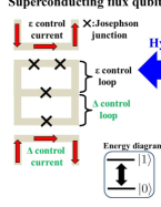
Figure 1: Illustration of the hybrid system composed of a superconducting flux qubit and an ensemble of NV^- centers. The flux qubit has four Josephson junctions that forms a two-level system. There are two control lines for the flux qubit. We use one of the control lines to change the energy bias $\epsilon$, and use the other line to change the energy gap $\Delta$. Diamond crystal is glued on top of a flux qubit, and this diamond contains NV^- centers. The electrons spins trapped in the NV^- center form a three-level system, and so we have a V-type energy level structure for the NV^- center.

It is often useful to transfer the state between the FQ and NV^- centers for quantum information processing. We keep quantum states in the quantum memory (NV^- centers) when gate operations are not required. On the other hand, to perform gate operations, we need to transfer the quantum states from the quantum memory to the quantum processor (FQ), which can be realized by using vacuum Rabi oscillation (VRO). However, the error rate of the state transfer in the current technology is an order of ten percent Kubo and et al (2011); Zhu et al. (2011); Saito et al. (2013), which is too large to perform quantum computation Raussendorf et al. (2007); Stephens et al. (2013). The noise mainly comes from the inhomogeneous broadening of the NV^- centers. Therefore, it is crucial to suppress the decoherence of the NV^- centers for computational tasks.

Improving the coherence time of the NV^- center ensemble also has a fundamental importance in the area of quantum metrology Pham et al. (2011); Hardal et al. (2013), quantum walk Hardal et al. (2013), and quantum simulation Yang et al. (2012). In these applications, the efficiency strongly depends on the coherence time of the ensemble of NV^- centers. So it is essential in these areas to find a way to improve the coherence time of the NV^- centers.

A cavity protection Putz and et al (2014); Krimer and et al (2014); Diniz and et al (2011) is a promising way to improve the coherence time of the NV^- center ensemble. If the coupling strength between the ensemble of NV^- centers and a superconducting flux qubit (or microwave cavity) is larger than the inhomogeneous width of the NV^- centers, the collective mode of the NV^- centers could be well decoupled from the other sub-radiant states of the NV^- so that inhomogeneous broadening would be suppressed. However, it has been shown that, if the spectral density of the inhomogeneous broadening is described by a Lorentzian, the noise cannot be suppressed by the cavity protection Diniz and et al (2011); Kurucz et al. (2011). Moreover, for the applications of quantum memory and quantum field sensing, it is sometime necessary to turn off the interaction between the NV centers and superconducting circuit. So it is better to have an alternative scheme that will work even for such cases.

In this paper, we report an improvement of the lifetime of the VRO by applying an in-plain magnetic field to this hybrid system. We have observed VRO with/without the magnetic field, and the lifetime of the VRO with magnetic field is nearly twice than without magnetic field. We have constructed a theoretical model to reproduce these results, and have found that the magnetic field suppress the inhomogeneous strain effect.

Let us now describe our experimental set-up. Our system consists of a gap-tunable FQ Paauw et al. (2009); Zhu et al. (2010) on which a diamond crystal with NV^- density of approximately $5\times 10^{17}$ cm^-3 is bonded Saito et al. (2013). The NV^- ensemble is created by the ion implantation and annealing in in vacuum Zhu et al. (2011); Saito et al. (2013). The distance between the FQ and the surface of the diamond crystal is less than $1\mu m$. We can apply external magnetic field of 2.6 mT along the [100] crystalline axis Saito et al. (2013). The gap-tunable FQ is fabricated with a superconducting loop containing four Josephson junctions. To control the FQ, a microwave line is fabricated around the FQ. The FQ is designed to couple with the SQUID structure via magnetic fields. The probability of the excited state of the FQ is measured by the SQUID.

To observe the VRO, we perform the following experiment. First, we excited the FQ by applying microwave pulse where the FQ is decoupled from the NV^- centers by the detuning. Second, we brought the FQ into the resonance of the NV$-$ centers by applying a magnetic flux. Finally, after a time $t$, we can measure the excited probability of the FQ via the SQUID. The measurements were done in a dilution refrigerator at a temperature below 50 mK.

We describe our system by the Hamiltonian Diniz and et al (2011); Marcos and et al (2010); Kubo and et al (2011); Zhu et al. (2014)

$$H=H_{\text{flux}}+H_{\text{int}}+H_{\text{ens}}\ \ \ \ \ \ \ \ \ \ \ \ \ \ \ \ \ \ \ \ \ \ \ \ \$$ (1)

$$H_{\text{flux}}=\frac{\hbar}{2}{\color[rgb]{0,0,0}\Delta}\hat{\sigma}_{z}+\frac{\hbar}{2}{\color[rgb]{0,0,0}\epsilon}\hat{\sigma}_{x},\ \ \ \ \ \ \ \ \ \ \ \ \ \ \ \ \ \ \ \ \ \ \ \$$ (2)

$$H_{\text{int}}=\hbar g_{e}\mu_{B}\hat{\sigma}_{x}\Big{(}\sum_{k=1}^{N}{\bf{B}}^{(k)}_{\text{qb}}\cdot{\bf{S}}_{k}\Big{)}\ \ \ \ \ \ \ \ \ \ \ \ \ \ \ \ \ \ \$$ (3)

$$H_{\text{ens}}=\Big{(}\sum_{k=1}^{N}\hbar D_{k}\hat{S}^{2}_{z,k}+\hbar E^{(k)}_{1}(\hat{S}^{2}_{x,k}-\hat{S}^{2}_{y,k})$$ (4)

$$+\hbar E^{(k)}_{2}(\hat{S}_{x,k}\hat{S}_{y,k}+\hat{S}_{y,k}\hat{S}_{x,k})+\hbar g_{e}\mu_{B}{\bf{B}}^{(k)}_{\text{NV}}\cdot{\bf{S_{k}}}\Big{)}$$ (5)

where $\hat{\sigma}_{x,y,z}$ denotes the Pauli matrix for FQ with $\hat{\sigma}_{x}$ whose eigenstates corresponds to two persistent-current states. Also, we define $\hat{\sigma}_{\pm}=\frac{1}{2}(\hat{\sigma}_{x}\pm i\hat{\sigma}_{y})$. The electron spin 1 operators of the NV^- center are represented by $\hat{S}_{x,y,z}$. $H_{\text{flux}}$ denotes the Hamiltonian of the FQ where $\Delta$ denotes the energy gap and $\epsilon$ denotes the magnetic energy bias. $H_{\rm{ens}}$ represents the ensemble composed of $N$ individual NV^- centers where $D/2\pi\simeq 2.878$GHz denotes a zero field splitting, $E_{k}=\sqrt{(E^{(k)}_{1})^{2}+(E^{(k)}_{2})^{2}}$ denotes a strain induced splitting, $g_{e}\mu_{B}{\bf{B}}_{\text{NV}}\cdot{\bf{S}}$ denotes a Zeeman splitting, and $\bf{B}_{\text{NV}}$ denotes a magnetic field with $g_{e}\mu_{B}/2\pi=28$MHz$\cdot$mT^-1. A quantization axis (z axis) to be the direction from the vacancy to the nitrogen is set by the zero field splitting of the NV^- center. For a small magnetic field $D\gg g_{e}\mu_{B}|{\bf{B}}_{\text{NV}}|$, the x and y component of the magnetic field is insignificant to change quantized axis of the NV^- center, and so we include only the effect of z axis of the field. We consider three relevant type of the magnetic field ${\bf{B}}_{\text{NV}}$: an in-plane external magnetic field $B_{\text{ex}}$, an inhomogeneous magnetic field due to P1 centers $B_{\text{inh}}$, and a hyperfine field from the nitrogen nuclear spins $B_{\text{hf}}$. The term $H_{\rm int}$ denotes the magnetic coupling between the FQ and the NV^- centers where ${\bf{B}}^{(k)}_{\text{qb}}$ represented the magnetic field induced by persistent current of the FQ. Since collective enhancement of the coupling strength between the NV^- and FQ is not available along the z axis of the NV^- center Marcos and et al (2010), we can ignore the coupling with $\hat{S}_{z}$. We can write $H_{\text{int}}$ as $H_{\text{int}}=\hbar\sum_{k=1}^{N}g\hat{\sigma}_{x}\cdot(\hat{S}_{x,k}\cos\phi_{k}-\hat{S}_{y,k}\sin\phi_{k})$ where $g=g_{e}\mu_{B}B^{(xy)}_{\text{qb}}$ denotes a Zeeman splitting of the NV^- spin due to FQ magnetic field $B^{(xy)}_{\text{qb}}$ in x-y plane and $\phi_{k}$ denotes the angle of the field in the plane.

For an ensemble of NV^- center with only a few excitations in it at most, we can use the Holstein-Primakoff approximation to treat NV^- spins as an ensemble of harmonic oscillators Houdré et al. (1996). We define creation (destruction) operators of a bright state and a dark state of the NV center Zhu et al. (2014) by $\hat{b}_{k}^{\dagger}=|A_{+}\rangle_{k}\langle 0|$ and $\hat{d}_{k}^{\dagger}=|A_{-}\rangle_{k}\langle 0|$, ($\hat{b}_{k}=|0\rangle_{k}\langle A_{+}|$ and $\hat{d}_{k}=|0\rangle_{k}\langle A_{-}|$) where $|A_{+}\rangle_{k}=\frac{\cos\phi_{k}}{\sqrt{2}}(|1\rangle_{k}+|-1\rangle_{k})+\frac{i\sin\phi_{k}}{\sqrt{2}}(|1\rangle_{k}-|-1\rangle_{k})$, $|A_{-}\rangle_{k}=\frac{i\sin\phi_{k}}{\sqrt{2}}(|1\rangle_{k}+|-1\rangle_{k})+\frac{\cos\phi_{k}}{\sqrt{2}}(|1\rangle_{k}-|-1\rangle_{k})$. Here, $|A_{+}\rangle_{k}\langle 0|$ denotes the state of the NV^- center to be directly coupled with the FQ while $|A_{-}\rangle_{k}\langle 0|$ has no direct coupling with the FQ. Since we consider only one or zero excitation in a total system, we can also replace a ladder operator of the FQ with a creation operator of a harmonic oscillator as $\hat{\sigma}_{+}\rightarrow\hat{c}^{\dagger}$.

Moving to a rotating frame with angular frequency $\omega$ defined by $U=e^{-i(\frac{1}{2}\omega\hat{\sigma}_{z}+\omega\hat{S}_{z}^{2})t}$ and making the rotating wave approximation, we obtain the simplified Hamiltonian $H\simeq\hbar\omega_{c}\hat{c}^{\dagger}\hat{c}+\sum_{k=1}^{N}\Big{(}\hbar\omega^{(k)}_{b}\hat{b}_{k}^{\dagger}\hat{b}_{k}+\hbar\omega^{(k)}_{d}\hat{d}_{k}^{\dagger}\hat{d}_{k}+\hbar g^{\prime}(\hat{c}^{\dagger}\hat{b}_{k}+\hat{c}\hat{b}_{k}^{\dagger})+\hbar(J_{k}+iJ^{\prime}_{k})\hat{b}_{k}^{\dagger}\hat{d}_{k}+\hbar(J_{k}-iJ^{\prime}_{k})\hat{b}_{k}\hat{d}_{k}^{\dagger}\Big{)}$ where $\omega_{c}=\sqrt{\epsilon^{2}+\Delta^{2}}$, $\omega^{(k)}_{b}\simeq D_{k}-\omega-E_{y,k}$, $\omega^{(k)}_{d}\simeq D_{k}-\omega+E_{y,k}$, $J_{k}=g_{e}\mu_{B}B^{(k)}_{z}$, $J_{k}^{\prime}=E_{x,k}$, $g^{\prime}=g\Delta/\sqrt{\epsilon^{2}+\Delta^{2}}$, $E_{x,k}=E_{k}\cos 2\phi_{k}$, and $E_{y,k}=E_{k}\sin 2\phi_{k}$.

Now the dynamics of this hybrid system can be investigated using the Heisenberg equations of motions. We write Heisenberg equations of motion as

$$\frac{d}{dt}\hat{c}=-i\omega_{c}\hat{c}-i(\sum_{k=1}^{N}g_{k}\sin\xi\cdot\hat{b}_{k})-\Gamma_{c}\hat{c}\ \ \ \ \ \ \ \ \$$ (6)

$$\frac{d}{dt}\hat{b}_{k}=-i\omega^{(k)}_{b}\hat{b}_{k}-iJ_{k}\hat{d}_{k}+J^{\prime}_{k}\hat{d}_{k}-ig\sin\xi_{k}\cdot\hat{c}-\Gamma_{b}\hat{b}_{k}$$ (7)

$$\frac{d}{dt}\hat{d}_{k}=-i\omega^{(k)}_{d}\hat{d}_{k}-iJ_{k}\hat{b}_{k}-J^{\prime}_{k}\hat{b}_{k}-\Gamma_{d}\hat{d}_{k}\ \ \ \ \ \ \ \ \$$ (8)

where $\Gamma_{c}$, $\Gamma_{b}$, and $\Gamma_{d}$ denote the decay rate of $\hat{c}$, $\hat{b}$, and $\hat{d}$, respectively. We numerically solve these equations with an initial state of $|\psi(t=0)\rangle=\hat{c}^{\dagger}|\text{vac}\rangle$, and plot the renormalized excitation probability of the FQ (which corresponds a switching probability of SQUID) in the Fig. 2 and Fig. 3.

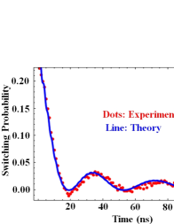
Figure 2: Vacuum Rabi oscillations between the FQ and NV^- centers without an applied external magnetic field. Red dots show the experimental results while the blue line shows the results of a numerical model where we use $N=1200$, $\epsilon=0$, $\Gamma_{c}/2\pi=0.3$MHz, $\Gamma_{b}/2\pi=\Gamma_{d}/2\pi=0.44$MHz, $\delta D_{k}/2\pi=0.08$MHz (FWHM), $\delta(g\mu_{B}B^{(k)}_{z})/2\pi=3.1$MHz(FWHM), $\delta E_{1,k}/2\pi=\delta E_{2,k}/2\pi=4.4$MHz(FWHM), $A_{HF}=2.3$MHz, and $\sqrt{N}g/2\pi=13$MHz

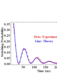
Figure 3: Vacuum Rabi oscillations between the FQ and NV^- centers with an applied external magnetic field of $2.6$ mT along the [100] crystalline axis. Except the magnetic field, we use the same parameters as those in Fig. 2.

Now let us detail our simulation technique and the core elements of it. The Lorentzian distributions, which have been typically used to describe the inhomogeneous broadening of the NV^- centers Zhu et al. (2011, 2014); Kubo and et al (2011); Kubo and et al (2012b), are assumed for $D^{(k)}_{0}$, $E_{1,k}$, and $E_{2,k}$ $(k=1,2,\cdots,N)$ to include the effect of the inhomogeneous lattice distortion of the NV^- centers. Next, due to the electron spin-half bath in the environment such as P1 center, randomized magnetic field on the NV center exists, and the nitrogen nuclear spin splits the electron-spin energy into three level via a hyperfine coupling. To include both these two effect, we use a random distribution of the magnetic fields with the form of the mixture of three Lorentzian functions that are separated with $2\pi\times 2.3$ MHz due to the hyperfine interaction with ${}^{14}N$ nuclear spin Kubo and et al (2011); Saito et al. (2013). With these assumptions, we have reproduced the VRO with/without applied magnetic field in the Fig. 2 and Fig. 3. While the FQ can induce the transition both $|0\rangle_{k}\leftrightarrow|-1\rangle_{k}$ and $|0\rangle_{k}\leftrightarrow|1\rangle_{k}$ with zero applied magnetic field, the FQ induces only one of them with applied magnetic field of a few mT due to the detuning effect Kubo and et al (2010); Zhu et al. (2011); Marcos and et al (2010); Saito et al. (2013); Diniz and et al (2011). This changes the effective coupling strength between the FQ and NV centers, and is the cause of the different time interval of the oscillations in the Fig. 2 and Fig. 3. With an applied magnetic field of 2.6 mT, the VRO can be observed until around $170$ ns while we cannot observe a clear oscillation beyond $100$ ns without an applied magnetic field. Thus, it shows the external magnetic field improves the lifetime of the VRO.

We explain how we determine the parameters for the numerical simulations. $\Gamma_{c}$ can be determined by the $T_{1}$ measurement of the FQ, which was performed independent of the VRO experiment Saito et al. (2013). Since the frequency shift of $E$ is 50 times larger than that of $D$ when an electric field is applied Dolde and et al (2011), we use $\delta E\simeq 50\delta D$ in this paper. It is known that, from the spectroscopic measurements, a sharp peak located in the middle of the avoided crossing structure was observed in this hybrid system Zhu et al. (2014), and one can determine the $\Gamma_{b}(=\Gamma_{d})$ from the width of this sharp peak Zhu et al. (2014). The time period of the VRO let us specify the value of $\sqrt{N}g$. Moreover, as we describe later, the envelope of the VRO with (without) magnetic field is mainly determined by $\delta B_{z}$ ($\delta B_{z}$ and $\delta E$). So, by fitting the spectroscopy and VRO with/without magnetic field, one can specify necessary parameters for our model.

We understand why the applied magnetic field actually improves the coherence time of the NV^- centers. There are two relevant decoherence source for the NV centers, inhomogeneous magnetic fields and the strain distribution Zhu et al. (2011); Kubo and et al (2011); Saito et al. (2013). The magnetic-field noise comes from an effective Hamiltonian between P1 center and NV center as $H_{\text{eff}}=\sum_{k,l}\lambda_{k,l}\hat{\sigma}^{(\text{P1},l)}_{z}\hat{S}^{(k)}_{z}$ where flip-flop term is negligible due to the large energy difference between them. However, this term commutes with the Zeeman term of the applied external magnetic field as $g_{e}\mu_{B}B_{\text{ex}}\hat{S}_{z}$, and so external magnetic field cannot affect this. On the other hand, the Hamiltonian of the inhomogeneous strain does not commute with the Zeeman Hamiltonian of the applied external magnetic field. Actually, the Hamiltonian of the $k$ th NV^- center is written as $H^{(k)}_{\text{NV}}=\hbar\omega^{(k)}_{b}\hat{b}_{k}^{\dagger}\hat{b}_{k}+\hbar\omega^{(k)}_{d}\hat{d}_{k}^{\dagger}\hat{d}_{k}+\big{(}(J_{k}+iJ^{\prime}_{k})\hat{b}^{\dagger}_{k}\hat{d}_{k}+\text{e.c}\big{)}$, and the eigenenergies are $E_{0}=0$ and $E_{\pm}=D\pm\sqrt{E^{2}_{x,k}+E^{2}_{y,k}+(g_{e}\mu_{B}B_{z}^{(k)})^{2}}$. If the magnetic field is large, we can expand the eigenenergies of the excited states as $E_{+}\simeq g_{e}\mu_{B}B^{(k)}_{z}\pm\frac{E^{2}_{x,k}+E^{2}_{y,k}}{2g_{e}\mu_{B}B^{(k)}_{z}}$. So the effect of the variations of $E_{x,k}$ and $E_{y,k}$ becomes negligible, and this could improve the lifetime of the VRO .

To confirm this effect, we performed another numerical simulation of the VRO with applied magnetic field for the strain values of $\delta E/2\pi=4.4,6.0,7.6$ MHz in the Fig. 4. Interestingly, the three VROs shown in the Fig. 4 are almost the same. These results clearly show that the lifetime of the VRO is quite robust against the inhomogeneous strains. So we conclude that the external magnetic field suppress the effect of inhomogeneous strain so that the improvement of the lifetime has been observed in our experiment. It is worth mentioning that, although possible suppression of the strain distribution by the applied magnetic field is mentioned in Acosta et al. (2013), we firstly demonstrate such a mechanism by the experiment.

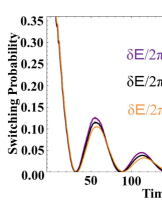
Figure 4: Numerical simulations of vacuum Rabi oscillations with the applied magnetic field for several values of the strains. Except the values of the strains, we use the same parameters as those in Fig. 3.

It is known that applying transversal magnetic field can improve the coherence time of the NV^- centers when the strain distribution is much larger than the decoherence rate due to the randomized magnetic fields Shin and et al (2013). Here, the application of the transversal magnetic field can suppress the decoherence due to the environmental magnetic field while this cannot suppress the inhomogeneous broadening of the strain Shin and et al (2013). On the other hand, our scheme to apply horizontal magnetic field is complemental to this, because we can suppress the strain inhomogeneous broadening. Our scheme has an advantage especially when we can decrease the broadening due to the magnetic field by using another technique.

Actually, it is possible to combine our scheme with another technique to reduce the inhomogeneous magnetic fields. For example, one way to suppress the magnetic noise for the NV^- centers is to decrease the P1 centers (a nitrogen atom substituting a carbon atom) by using differently synthesized diamond crystals Saito et al. (2013). P1 centers are considered as a electron spin-half bath, and they cause randomized magnetic field to decoher the NV^- centers Kubo and et al (2011); Zhu et al. (2011). However, reduction of the P1 centers cannot suppress the noise due to the strain. Therefore, by applying a magnetic field with a diamond having less P1 centers, further improvement of the coherence time should be possible. This provides us with a sensitive diamond-based field sensor, and will be useful for a long-lived quantum memory during quantum computation as future applications.

In conclusion, we have observed an improvement of a lifetime of the vacuum Rabi oscillations between the FQ and NV centers by applying an in-plain magnetic field. By reproducing the experimental result from a theoretical model, we have found that the applied magnetic field can suppress the inhomogeneous broadening of the strain. This result is a relevant step toward to the realization of the long-lived quantum memory for a superconducting flux qubit.

We thank R. Amsüss and H. Nakano for valuable discussions. This work was supported by KAKENHI(S) 25220601 and in part by Commissioned Research of NICT.

References

- Wallquist and et al (2009) M. Wallquist and et al , Physica Scripta 2009, 014001 (2009).
- Xiang and et al (2013) Z.-L. Xiang and et al , Reviews of Modern Physics 85, 623 (2013).
- Imamoğlu (2009) A. Imamoğlu, Phys. Rev. Lett. 102, 083602 (2009).
- Wesenberg and et al (2009) J. Wesenberg and et al , Phys. Rev. Lett. 103, 70502 (2009).
- Schuster and et al (2010) D. Schuster and et al , Phys. Rev. Lett. 105, 140501 (2010).
- Wu and et al (2010) H. Wu and et al , Phys. Rev. Lett. 105, 140503 (2010).
- Kubo and et al (2010) Y. Kubo and et al , Phys. Rev. Lett. 105, 140502 (2010).
- Amsüss and et al (2011) R. Amsüss and et al , Phys. Rev. Lett. 107, 060502 (2011).
- Kubo and et al (2011) Y. Kubo and et al , Phys. Rev. Lett. 107, 220501 (2011).
- Zhu et al. (2011) X. Zhu, S. Saito, A. Kemp, K. Kakuyanagi, S. Karimoto, H. Nakano, W. Munro, Y. Tokura, M. Everitt, K. Nemoto, et al., Nature 478, 221 (2011).
- Kubo and et al (2012a) Y. Kubo and et al , Phys. Rev. A 85, 012333 (2012a).
- Kubo and et al (2012b) Y. Kubo and et al , Phys. Rev. B 86, 064514 (2012b).
- Marcos and et al (2010) D. Marcos and et al , Phys. Rev. Lett. 105, 210501 (2010).
- Twamley and Barrett (2010) J. Twamley and S. Barrett, Physical Review B 81, 241202 (2010).
- Matsuzaki and Nakano (2012) Y. Matsuzaki and H. Nakano, Physical Review B 86, 184501 (2012).
- Saito et al. (2013) S. Saito, X. Zhu, R. Amsüss, Y. Matsuzaki, K. Kakuyanagi, T. Shimo-Oka, N. Mizuochi, K. Nemoto, W. J. Munro, and K. Semba, Phys. Rev. Lett. 111, 107008 (2013).
- Julsgaard and et al (2013) B. Julsgaard and et al , Phys. Rev. Lett. 110, 250503 (2013).
- Diniz and et al (2011) I. Diniz and et al , Phys. Rev. A 84, 063810 (2011).
- Zhu et al. (2014) X. Zhu, Y. Matsuzaki, R. Amsuss, K. Kakuyanagi, T. Shimo-Oka, N. Mizuochi, K. Nemoto, W. J. Munro, K. Semba, and S. Saito, Nature communications 3424, 4524 (2014).
- Sandner et al. (2012) K. Sandner, H. Ritsch, R. Amsüss, C. Koller, T. Nöbauer, S. Putz, J. Schmiedmayer, and J. Majer, Physical Review A 85, 053806 (2012).
- Clarke and Wilhelm (2007) J. Clarke and F. Wilhelm, Nature 453, 1031 (2007).
- Bylander and et al (2011) J. Bylander and et al , Nature Physics 7, 565 (2011).
- Stern et al. (2014) M. Stern, G. Catelani, Y. Kubo, C. Grezes, A. Bienfait, D. Vion, D. Esteve, and P. Bertet, Phys. Rev. Lett. 113, 123601 (2014).
- Balasubramanian and et al (2009) G. Balasubramanian and et al , Nature materials 8, 383 (2009).
- Takahashi et al. (2008) S. Takahashi, R. Hanson, J. Van Tol, M. S. Sherwin, and D. D. Awschalom, Physical review letters 101, 047601 (2008).
- Mizuochi et al. (2009) N. Mizuochi, P. Neumann, F. Rempp, J. Beck, V. Jacques, P. Siyushev, K. Nakamura, D. Twitchen, H. Watanabe, S. Yamasaki, et al., Physical review B 80, 041201 (2009).
- Ishikawa et al. (2012) T. Ishikawa, K.-M. C. Fu, C. Santori, V. M. Acosta, R. G. Beausoleil, H. Watanabe, S. Shikata, and K. M. Itoh, Nano letters 12, 2083 (2012).
- Maurer et al. (2012) P. Maurer, G. Kucsko, C. Latta, L. Jiang, N. Yao, S. Bennett, F. Pastawski, D. Hunger, N. Chisholm, M. Markham, et al., Science 336, 1283 (2012).
- Bar-Gill et al. (2013) N. Bar-Gill, L. M. Pham, A. Jarmola, D. Budker, and R. L. Walsworth, Nature communications 4, 1743 (2013).
- Kurucz et al. (2011) Z. Kurucz, J. Wesenberg, and K. Mølmer, Physical Review A 83, 053852 (2011).
- Raussendorf et al. (2007) R. Raussendorf, J. Harrington, and K. Goyal, New J. Phys. 9, 199 (2007), eprint quant-ph/0703143.
- Stephens et al. (2013) A. M. Stephens, W. J. Munro, and K. Nemoto, Physical Review A 88, 060301 (2013).
- Hardal et al. (2013) A. Ü. Hardal, P. Xue, Y. Shikano, Ö. E. Müstecaplıoğlu, and B. C. Sanders, Physical Review A 88, 022303 (2013).
- Pham et al. (2011) L. M. Pham, D. Le Sage, P. L. Stanwix, T. K. Yeung, D. Glenn, A. Trifonov, P. Cappellaro, P. Hemmer, M. D. Lukin, H. Park, et al., New Journal of Physics 13, 045021 (2011).
- Yang et al. (2012) W. Yang, Z.-q. Yin, Z. Chen, S.-P. Kou, M. Feng, and C. Oh, Physical Review A 86, 012307 (2012).
- Putz and et al (2014) S. Putz and et al , Nature Physics 10, 720 (2014).
- Krimer and et al (2014) D. O. Krimer and et al , Physical Review A 90, 043852 (2014).
- Paauw et al. (2009) F. Paauw, A. Fedorov, C. M. Harmans, and J. Mooij, Phys. Rev. Lett. 102, 090501 (2009).
- Zhu et al. (2010) X. Zhu, A. Kemp, S. Saito, and K. Semba, Applied Physics Letters 97, 102503 (2010).
- Houdré et al. (1996) R. Houdré, R. Stanley, and M. Ilegems, Physical Review A 53, 2711 (1996).
- Dolde and et al (2011) F. Dolde and et al , Nature Physics 7, 459 (2011).
- Acosta et al. (2013) V. Acosta, D. Budker, P. Hemmer, J. Maze, and R. Walsworth, Optical magnetometry (Cambridge University Press) (2013).
- Shin and et al (2013) C. S. Shin and et al , Physical Review B 88, 161412 (2013).