A Bayesian Change Point Model for Detecting Land Cover Changes in MODIS Time Series

Abstract

As both a central task in Remote Sensing and a common problem in many other situations involving time series data, change point detection boasts a thorough and well-documented history of study. However, the treatment of missing data and proper exploitation of the structure in multivariate time series during change point detection remains lacking. Multispectral, high temporal resolution time series data from NASA’s Moderate Resolution Imaging Spectroradiometer (MODIS) instruments provide an attractive and challenging context to contribute to the change point detection literature. In an effort to better monitor change in land cover using MODIS data, we present a novel approach to identifying periods of time in which regions experience some conversion-type of land cover change. That is, we propose a method for parameter estimation and change point detection in the presence of missing data which capitalizes on the high dimensionality of MODIS data. We test the quality of our method in a simulation study alongside a contemporary change point method and apply it in a case study at the Xingu River Basin in the Amazon. Not only does our method maintain a high accuracy, but can provide insight into the types of changes occurring via land cover conversion probabilities. In this way we can better characterize the amount and types of forest disturbance in our study area in comparison to traditional change point methods.

,,, and

1 Introduction

To enhance and inform Earth system models, timely and accurate monitoring of land cover must be maintained (Bonan et al., 2002; Ek et al., 2003; Running and Coughlan, 1988; Sterling and Ducharne, 2008). Additionally, because the land area affected by humans has expanded rapidly (Ellis and Ramankutty, 2008; Goldewijk, 2001; Ramankutty and Foley, 1999; Sanderson et al., 2002; Vitousek et al., 1997) and society depends to a large extent on terrestrial ecosystems (Foley et al., 2005), high quality information regarding changes in land cover is crucial for modern land-use policy and natural resource management.

Remote sensing instruments onboard various satellite platforms have been providing repeated observation of the Earth’s surface, enabling continuous mapping and monitoring of land cover change, especially those caused by human activities. With continuous missions, some instrument series have observations over the past few decades (e.g., the Landsat series, the Advanced Very High Resolution Radiometer (AVHRR) series). A unique sensor named the Moderate Resolution Imaging Spectroradiometer (MODIS), has been in orbit onboard NASA’s Terra and Aqua satellites since the early 2000s. This instrument strikes a balance between moderate spatial resolution (250–500 meters) and high revisit capability, providing time series observations for over a decade. However, a host of issues plagues MODIS data such as measurement errors, atmospheric contamination, and variable view geometry and gridding artifacts (Roy, 2000; Huang et al., 2002; Tan et al., 2006), and renders change detection a challenging task due to missing and noisy data.

Various change detection techniques were developed using bi-temporal or multi-temporal imagery for mapping changes including deforestation, forest mortality, and urban expansion (see (Singh, 1989; Rogan et al., 2002; Coppin et al., 2004; Lu et al., 2004)). As MODIS time series grow, more studies have focused on better exploitation of the temporal information in MODIS data for change detection, e.g. (Verbesselt et al., 2010; Rahman et al., 2013; Huang and Friedl, 2014). However, due to the volume of data and nature of optical remote sensing (susceptible to cloud and atmospheric contamination), it remains challenging to pre-process and fully utilize the time series data. Thus, there is great need of methods that (i) better address missing data; that (ii) explore the rich structure in the data in their spectral, temporal, and spatial dimensions; and that (iii) are robust to noise.

Most existing methods for change detection in the presence of missing data attempt to impute or estimate missing data first and then proceed to identify changes (Lunetta et al., 1999; Lunetta et al., 2006; Boriah, 2010). Estimation can proceed in a number of ways, including, for example, nearest neighbor interpolation (Ning and Cheng, 2012; Zhang, 2012; Jerez et al., 2010) or linear, polynomial, or spline interpolation (Junninen et al., 2004). Missing values can be imputed using multiple imputation (Honaker and King, 2010) or expectation-maximization (EM) (Dempster et al., 1977) (for a thorough review of handling missing data in statistical analyses, see (Little and Rubin, 2002).) However, since missing data are often handled separately from and prior to change point estimation, the imputation does not account for possible large changes and so the resulting change detection can lack statistical power.

In this paper we introduce and assess a novel, off-line change point detection model that is tailored to the data characteristics of MODIS time series, i.e. large and structured. Our key contribution is to characterize change as transitions in land cover: we assume that the region of study is reasonably homogeneous, with a predominant “background” land cover class, and we evaluate change by implicitly classifying land cover and contrasting estimated classes to the background. This way, we can not only detect changes but also understand their nature; for instance, we can better assess if native forest was burned, logged, or converted to cropland. By exploiting land cover information from training data, we specify a Bayesian hierarchical model to detect distributional, conversion-type changes in multispectral time series while accounting for missing data. In addition, as opposed to at-most-one-change (AMOC) models that aim at detecting single abrupt disruptions, our formulation allows for at most two change points and thus also considers possible recovery from prior disturbances. We describe the change point detection model in Section 2, and we apply and evaluate our model using a simulation study (Section 3.1) and a case study (Section 3.2).

1.1 Data Description

To illustrate the main issues that afflict MODIS data, here we describe the dataset that is used in the case study of Section 3.2. We use the MODIS 500 meter Nadir BRDF-adjusted Reflectance (NBAR) product, which is designed to minimize noise due to bidirectional reflectance effects arising from varying solar and view geometry (Schaaf et al., 2002). This product features seven spectral bands designed for land observation, covering visible to shortwave infrared wavelengths (Survey, 2013).

For each pixel in the region of interest and for each year in the dataset—from 2001 to 2010—we originally obtained time series of 46 NBAR composite values for seven spectral bands. However, for our analysis we select a temporal subset of 19 observations per year (May to September) in order to exclude the wet season and reduce the proportion of missing data. Here it is essential to treat years as the main temporal unit to keep seasonality effects, including phenology, that characterize land cover classes. We have verified that this subset still keeps enough seasonality within the year to distinguish well between classes.

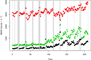
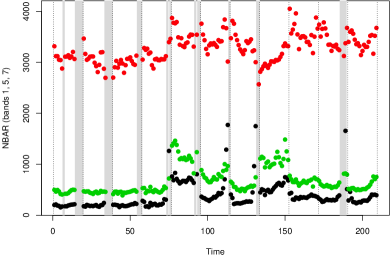
As an example, consider the spectro-temporal profiles for two representative pixels in Figure 1. To avoid overcrowding the plot, we only show three spectral bands (1, 5, and 7.) Gray bands mark missing data locations in at least one band. As we can see, most years have at least one time with missing values, and so discarding whole years is unfeasible. Moreover, since missing data happens more frequently at the end of our annual time series (i.e. start of wet season), it makes it harder to spot change between years. Some changes are more evident, as shown in the left plot at year 6, but some are harder to flag and can be attributed to minor disturbances, as in the right plot, at year 5. The right plot also highlights the possibility of recovery: the data profile seems to have returned to its background land cover state after year 9.

Figure 1: Spectral-temporal profiles for two representative pixels in a study area, bands 1 (black), 5 (red), and 7 (green.) Gray horizontal lines mark missing data in at least one spectral band. Reflectance values have been multiplied by 10000.

Land cover change detection requires a scheme of land cover classes which encompasses all major land cover types. We employ a carefully established set of land cover classes constructed under the International Geosphere-Biosphere Programme (IGBP) (Davis and Holmgren, 2000), as defined in Table 1.

Table 1: Land cover class definitions within the International Geosphere-Biosphere Programme (IGBP.)

Class	Class name	Description
1	Evergreen Needleleaf Forests	Lands dominated by trees with a percent canopy cover $>$60$\%$ and height exceeding 2 meters. Almost all tree remain green all year. Canopy is never without green foliage.
2	Evergreen Broadleaf Forests	Lands dominated by trees with a percent canopy cover $>60\%$ and height exceeding 2 meters. Almost all tree remain green all year. Canopy is never without green foliage.
3	Deciduous Needleleaf Forests	Lands dominated by trees with a percent canopy cover $>$60$\%$ and height exceeding 2 meters. Consists of seasonal needleleaf tree communities with an annual cycle of leaf-on and leaf-off periods.
4	Deciduous Broadleaf Forests	Lands dominated by trees with a percent canopy cover $>$60$\%$ and height exceeding 2 meters. Consists of seasonal broadleaf tree communities with an annual cycle of leaf-on and leaf-off periods.
5	Mixed Forests	Lands dominated by trees with a percent canopy cover $>$60$\%$ and height exceeding 2 meters. Consists of tree communities with interspersed mixtures or mosaics of the other four forest cover types. None of the forest types exceeds 60$\%$ of landscape.
6	Closed Shrublands	Lands with woody vegetation less than 2 meters tall and with shrub canopy cover is $>$60$\%$. The shrub foliage can be either evergreen or deciduous.
7	Open Shrublands	Lands with woody vegetation less than 2 meters tall and with shrub canopy cover is 10–60$\%$. The shrub foliage can be either evergreen or deciduous.
8	Woody Savannas	Lands with herbaceous and other understorey systems, and with forest canopy cover between 30–60$\%$. The forest cover height exceeds 2 meters.
9	Savannas	Lands with herbaceous and other understorey systems, and with forest canopy cover between 10–30$\%$. The forest cover height exceeds 2 meters.
10	Grasslands	Lands with herbaceous types of cover. Tree and shrub cover is less than 10$\%$.
11	Permanent Wetlands	Lands with a permanent mixture of water and herbaceous or woody vegetation that cover extensive areas. The vegetation can be present in either salt, brackish, or fresh water.
12	Cropland	Lands covered with temporary crops followed by harvest and a bare soil period (e.g. single and multiple cropping systems). Note that perennial woody crops will be classified as the appropriate forest or shrub land cover type.
13	Urban and Built-Up	Lands covered by building and other man-made structures.
14	Cropland/Nat. Veg. Mosaics	Lands with a mosaic of croplands, forest, shrublands, and grasslands in which no one component comprises more than 60$\%$ of the landscape.
15	Snow and Ice	Lands under snow and/or ice cover throughout the year.
16	Barren	Lands exposed soil, sand, rocks, or snow and never has more than 10$\%$ vegetated cover during any time of the year.
17	Water Bodies	Oceans, seas, lakes, reservoirs, and rivers. Can be either fresh or salt water bodies.

1.2 Prior and Related Work

Change point detection methods have been applied extensively in various fields of environmental and climate monitoring, to problems such as rates of Tropical cyclone activity, precipitation and temperature trends, and fishery population regime change (Elsner et al., 2000; Chu and Zhao, 2004; Rodionov, 2005; Solow and Beet, 2005). Statistically, the general change point problem can be categorized into on-line (real time) (Fearnhead and Liu, 2007) and off-line (retrospective) frameworks. Additionally, approaches to change point detection typically involve specifying which types of change to look for. Previous methods for detecting change vary by the following change types: mean-type shifts (Shao and Zhang, 2010; Lund and Reeves, 2002), variance change (Galeano and Peña, 2007), or change in distribution (Basseville and Nikiforov, 1993; Lee, 2010; Tsay, 1988; Song et al., 2007; Gombay, 2008). Popular approaches include time series models, sequential testing, special forms of regression, and Bayesian techniques (Menzefricke, 1981; Booth and Smith, 1982; Stephens, 1994; Perreault et al., 2000; Fearnhead, 2006).

With continuous data collection and growing time series from the MODIS instruments, many studies in the remote sensing literature have put more emphasis on exploring temporal information for land cover change detection. Some of these methods detect change at the pixel level using change indices derived from annual time series (e.g., Linderman et al., 2005; Mildrexler et al., 2009; Coops et al., 2009). Other studies developed temporal trajectory-based change detection algorithms such as temporal segmentation, structural break test, and distance-metric based methods (e.g., Verbesselt et al., 2010; Sulla-Menashe et al., 2013; Huang and Friedl, 2014). While some of these methods have demonstrated feasibility for large area application, it remains challenging to pre-process the data for gap-free input and reduce spurious detection of change due to noise.

In this paper, we use the change detection method described in (Huang and Friedl, 2014) for comparison with our method. It is a distance metric-based change detection method for identifying changed pixels at annual time steps using 500 m MODIS NBAR time series data. The approach we describe uses distance metrics to measure (i) the similarity between a pixel’s annual time series to annual time series for pixels of the same land cover class, and (ii) the similarity between annual time series from different years at the same pixel. The combination of two distance metrics used both spatial (regional land cover related knowledge) and temporal information, and was shown to compare well with reference information derived from higher spatial resolution data. A set of essential pre-processing steps, including gap-filling, smoothing and temporal subsetting of MODIS 500 m NBAR time series, were also described as part of the approach.

2 Model and Methods

Consider, for each year $i=1,\ldots,J$, and each pixel $v$ in the region of interest $\mathscr{R}$, the vector observation $X_{iv}$ containing data from $B$ spectral bands and $T$ within-year time points. For example, in the data described in Section 1.1, $B=7$, $T=19$, and $J=10$. Since our data contain physical dimensions we exploit these features by partitioning the variation in the data into spectral and temporal components. Moreover, we expect land cover classes to have different mean profiles and different variances so we are able to distinguish them. Thus, if $\mathscr{C}$ is the set of land cover classes and $W_{v}\in\mathscr{C}$ codes for the land cover class of pixel $v$, we start by modeling the data using a matrix normal distribution (Dawid, 1981), or, equivalently,

$$X_{iv}{\,|\,}W_{v}=g\stackrel{{\scriptstyle\text{\tiny ind}}}{{\sim}}N(\mu_{g},\Sigma_{s}\otimes\Sigma_{tg}),$$ (1)

where $\otimes$ denotes the Kronecker product. That is, instead of assuming that our multivariate normal data have a single $BT\times BT$ covariance matrix we employ a Kronecker structured covariance matrix which isolates the spectral covariance in a $B\times B$ matrix, $\Sigma_{s}$, and the temporal covariance in a $T\times T$ matrix, $\Sigma_{tg}$. Note that we assume that spectral variation ($\Sigma_{s}$) transcends land cover class, and thus only allow the means ($\mu_{g}$) and temporal covariances ($\Sigma_{tg}$) to vary with land cover class $g$. In this way, we reduce the dimensionality of parameters to be estimated while keeping a parsimonious model structure (Glanz et al., 2014). In addition, since the temporal profiles $\mu_{g}$ capture seasonality and temporal variability is represented in $\Sigma_{tg}$, we do not need to explicitly model auto-correlation.

The separable nature of the variance also has the advantage of allowing us to reduce the dimensionality of the data using a focused PCA compression. If $\Sigma_{s}=P\text{Diag}(\lambda_{1:B})P^{\top}$ is the eigen-decomposition of $\Sigma_{s}$, we select the $K<B$ largest eigenvalues and, regarding $X_{iv}$ as a matrix with $B$ rows, we define a compressed version of $X_{iv}$ as

$$X^{*}_{iv}:={\text{Diag}(\lambda_{1:K})}^{-1}P_{1:K}^{\top}X_{iv}.$$ (2)

This transformation is equivalent to approximating $\Sigma_{s}$ using $K$ eigenvectors, $\Sigma_{s}\approx\Sigma_{s}^{*}:=P_{1:K}\text{Diag}(\lambda_{1:K})P_{1:K}^{\top}$, and decorrelating the columns of $X_{iv}$ by $\Sigma_{s}^{*}$.

Given the very large size of the data, we opt to learn land cover parameters $\mu_{g}$, $\Sigma_{s}$, and $\Sigma_{tg}$ in a pre-processing step instead of jointly with change point estimation. To this end, we adopt the EM method proposed in (Glanz et al., 2014) and apply it to an independent training dataset. This kind of prior elicitation is similar to empirical Bayes approaches (Carlin and Louis, 2000) and aims at simplifying the model and alleviating the computational burden of inference. To simplify the notation, for the remainder of this article we denote $\Sigma_{g}=\Sigma_{s}\otimes\Sigma_{tg}$.

While (1) gives a parametric model for the annual data at a pixel, we require a way to detect changes in land cover when these observations contain missing values. In pursuit of a change point year for each pixel, if it exists, we devise an EM algorithm which accounts for the missing data present throughout our region of interest. The following section details our hierarchical model and estimation procedure for identifying a change in land cover.

2.1 Change Point Hierarchical Model and Parameter Estimation

In our scenario, the annual data for each pixel, $X_{iv}$, are assumed to be conditionally independent of both data in other years at pixel $v$ as well as data and potential changes in other pixels. To model change, we allow the year sequence $1,\ldots,J$ to be segmented according to $\rho=(\rho_{1},\rho_{2})$, $1\leq\rho_{1}\leq\rho_{2}\leq J$, such that the segment $\rho_{1}+1,\ldots,\rho_{2}$ is in the “change” state, and the pre- and post-change segments $1,\ldots,\rho_{1}$ and $\rho_{2}+1,\ldots,J$ are in the “background” state. This way, if $\rho_{2}<J$ we have recovery from change to background. Lack of change is represented by $\rho_{1}=\rho_{2}=J$, the only case when $\rho_{1}=\rho_{2}$, that is, for any other configuration we have $\rho_{1}<\rho_{2}$.

For each pixel $v$, we assume the data in the background segment, i.e. up to the change point year $\rho_{1v}$ and after change point year $\rho_{2v}$, follow a multivariate normal distribution with mean $\mu_{0v}$, and the data in the change segment, i.e. from years $\rho_{1v}+1$ to $\rho_{2v}$, follow another multivariate normal distribution with mean $\mu_{cv}$. In addition, to accommodate more flexibility from pixel to pixel, we add a new level to our model and incorporate land cover class information via prior distributions for $\mu_{0v}$ and $\mu_{cv}$. Specifically, we set conjugate priors $\mu_{0v}\sim N(\mu_{F},\Sigma_{F})$ where $\mu_{F}$ and $\Sigma_{F}$ denote the mean and covariance of our background class, say Evergreen Broadleaf Forest (EBF); and $\mu_{cv}{\,|\,}W_{v}=g\sim N(\mu_{g},\Sigma_{g})$, where now $W_{v}\in\mathscr{C}$ indicates the land cover class to which pixel $v$ has transitioned in case of a change. The actual observations $X_{iv}$ now spread around $\mu_{0v}$ and $\mu_{cv}$ according to variance scales $\kappa_{0}$ and $\kappa_{c}$:

$$X_{iv}{\,|\,}\mu_{0v},\mu_{cv},\rho_{v}\stackrel{{\scriptstyle\text{\tiny ind}}}{{\sim}}I(i\in\text{BG}(\rho_{v}))N(\mu_{0v},\kappa_{0}I_{BT})+I(i\not\in\text{BG}(\rho_{v}))N(\mu_{cv},\kappa_{c}I_{BT}),$$ (3)

where $I(\cdot)$ is the indicator function, the background segment of $\rho_{v}$ is $\text{BG}(\rho_{v})=\{i:i\leq\rho_{1v}\text{~{}or~{}}i>\rho_{2v}\}$, and thus change positions $i\not\in\text{BG}(\rho_{v})$ correspond to $\rho_{1v}<i\leq\rho_{2v}$. Since the change affects the mean yearly temporal profiles $\mu_{0v}$ and $\mu_{cv}$, we can regard them as smoothed versions of $X_{iv}$ and so this hierarchical model is similar in spirit to the smoothing approach of Lunetta et al. (2006). However, since our interest does not lie in the mean profile parameters $\mu_{0v}$ and $\mu_{cv}$, we can further simplify our model by marginalizing them out to obtain:

$$X_{iv}{\,|\,}\rho_{v},W_{v}=g\stackrel{{\scriptstyle\text{\tiny ind}}}{{\sim}}I(i\in\text{BG}(\rho_{v}))N(\mu_{F},\Sigma_{F}+\kappa_{0}I_{BT})+I(i\not\in\text{BG}(\rho_{v}))N(\mu_{g},\Sigma_{g}+\kappa_{c}I_{BT}).$$

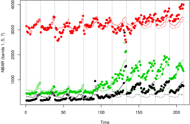
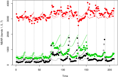
As an example, Figure 2 depicts $X_{iv}$ for the two representative pixels that were shown in Figure 1, along with estimated $\widehat{\mu}_{0v}$, $\widehat{\mu}_{cv}$, and $\widehat{\rho}_{v}$ using the EM method described in Section 2.2. For the pixel on the left panel, $\widehat{\rho}_{1v}=6$ and $\widehat{\rho}_{2v}=11$ (no recovery), while for the pixel on the right panel we have $\widehat{\rho}_{1v}=4$ and $\widehat{\rho}_{2v}=8$.

Figure 2: Spectral-temporal profiles for two representative pixels in study area along with estimated mean profiles for background and change land cover classes. Hollow points mark EM-imputed values. Dashed lines during change periods represent mean profiles under background land cover class for comparison. Reflectance values have been multiplied by 10000.

To set a weakly informative prior on $\rho_{v}$, we settle on a hierarchy that depends on two probabilities—the probability of a change occurring, $\pi_{0}$, and, given that a change occurred, the probability of recovery $\pi_{R}$—and we specify that configurations with the same number of change points are equally likely. Thus, the probabilities of no change, change without recovery (one change point), and change with recovery (two change points) are given, respectively, by

$$\begin{split}{\mathbb{P}}(\rho_{1v}=\rho_{2v}=J)&=1-\pi_{0},\\ {\mathbb{P}}(\rho_{1v}<\rho_{2v}=J)&=\frac{\pi_{0}(1-\pi_{R})}{J-1},~{}\text{and}\\ {\mathbb{P}}(\rho_{1v}<\rho_{2v}<J)&=\frac{\pi_{0}\pi_{R}}{\binom{J-1}{2}}.\\ \end{split}$$ (4)

Finally, we set $W_{v}{\,|\,}\boldsymbol{\alpha}\sim\text{\sf MN}(1,\boldsymbol{\alpha})$ to depend on a region-wise parameter $\boldsymbol{\alpha}$ that tells the a priori probability of changing to a certain class in $\mathscr{C}$, and elect a conjugate prior $\boldsymbol{\alpha}\sim\text{\sf Dir}(\boldsymbol{\pi})$. The specification of $\boldsymbol{\pi}$ provides an advantageous flexibility that we can exploit to inform the model of land cover classes we anticipate seeing after a change has occurred, making our approach particularly well suited for changes in the form of land cover conversions.

Our model can accommodate changes in mean or covariance and benefits from a Bayesian approach which incorporates potential a priori information about existence and location of a change point. Our ultimate goal with this model consists of inferring the change point locations $\rho_{v}$ for every pixel in the region of interest, a task we discuss next.

2.2 Identifying Change Points via Expectation-Maximization

To account for missing data, we partition the data in year $i$ and pixel $v$ as $X_{iv}=(Y_{iv},Z_{iv})$ where $Y_{iv}$ are actual observed data and $Z_{iv}$ are missing values. The missing entries $Z_{iv}$ can occur at multiple times within year $i$ and at multiple spectral bands, and these entries can vary from pixel to pixel. We assume that $Z_{iv}$ occur missing at random and represent them as $Z={\{Z_{iv}\}}_{i=1,\ldots,T,v\in\mathscr{R}}$ the whole collection of missing values in the dataset (and similarly for $Y=\{Y_{iv}\}$, the observed values.)

To estimate our parameters of interest $\Theta=\{{\{\rho_{v}\}}_{v\in\mathscr{R}},\boldsymbol{\alpha}\}$ we select a representative of the posterior distribution ${\mathbb{P}}(\Theta{\,|\,}Y)$ such as the maximum a posteriori (MAP) estimator

$$\widehat{\Theta}=\mathop{\rm arg\,max}\limits_{\Theta}\sum_{W}\int{\mathbb{P}}(\Theta,Z,W{\,|\,}Y)\,\text{d}Z=\mathop{\rm arg\,max}\limits_{\Theta}{\mathbb{P}}(\Theta{\,|\,}Y),$$ (5)

where $W={\{W_{v}\}}_{v\in\mathscr{R}\,:\,\rho_{1v}<J}$; that is, we marginalize the nuisance parameters $Z_{v}$, the missing values, and the change land class $W_{v}$ across all pixels $v\in\mathscr{R}$. While a traditional Bayesian approach relies on estimating ${\mathbb{P}}(\Theta{\,|\,}Y)$ using Markov chain Monte Carlo (MCMC) methods (Robert and Casella, 1999; Gelman et al., 2003), here we adopt an EM routine for computational expediency since we anticipate assessing change in large datasets that often comprise millions of pixels. Under this setup, we regard both $Z$ and $W$ as latent variables and wish to estimate directly the MAP in (5) by following a procedure that starts at some arbitrary $\Theta^{(0)}$ and iteratively updates

$$\begin{split}\Theta^{(t+1)}&=\mathop{\rm arg\,max}\limits_{\Theta}Q(\Theta,\Theta^{(t)}):=\mathop{\rm arg\,max}\limits_{\Theta}{\mathbb{E}}_{Z,W{\,|\,}Y;\Theta^{(t)}}\big{[}\log{\mathbb{P}}(\Theta,Z,W,Y)\big{]}\\ &=\mathop{\rm arg\,max}\limits_{\Theta}{\mathbb{E}}_{Z,W{\,|\,}Y;\Theta^{(t)}}\big{[}\log{\mathbb{P}}(\Theta,Z,W{\,|\,}Y)\big{]}\end{split}$$ (6)

until convergence. Function $Q$ computes the expectation (E) step, while the update in (6) performs the maximization (M) step.

In the spirit of a cyclic gradient descent approach, we alternate between updating the “global” parameter $\boldsymbol{\alpha}$ and then updating change points $\rho_{v}$ for each pixel $v$. This procedure is similar to a block version of an expectation conditional maximization (ECM) routine (Meng and Rubin, 1993). The details are as follows:

1. Start at arbitrary $\Theta^{(0)}$; for example, set $\alpha^{(0)}_{k}=\pi_{k}/\sum_{g\in\mathscr{C}}\pi_{g}$, for $k\in\mathscr{C}$, and $\rho^{(0)}_{1v}=\rho^{(0)}_{2v}=J$ for all pixels $v\in\mathscr{R}$.

2. For $t=1,2,\ldots$ (until convergence) do

   1. For $k\in\mathscr{C}$ do: update

      $$\alpha_{k}^{(t+1)}=\frac{\sum_{v\,:\,\rho_{1v}^{(t)}<J}{\mathbb{P}}(W_{v}=k{\,|\,}Y_{v};\Theta^{(t)})+\pi_{k}-1}{N_{v}^{(t)}+\sum_{g\in\mathscr{C}}\pi_{g}-|\mathscr{C}|},$$ (7)

      where $N_{v}^{(t)}=|\{v\,:\,\rho_{1v}^{(t)}<J\}|$ is the number of pixels with changes and

      $${\mathbb{P}}(W_{v}=k{\,|\,}Y_{v};\Theta^{(t)})=\frac{\alpha_{k}^{(t)}{\mathbb{P}}(Y_{v}{\,|\,}W_{v}=k;\Theta^{(t)})}{\sum_{g\in\mathscr{C}}\alpha_{g}^{(t)}{\mathbb{P}}(Y_{v}{\,|\,}W_{v}=g;\Theta^{(t)})}.$$ (8)

      We note that if we denote by ${\text{\sf miss}}(X)$ and $-{\text{\sf miss}}(X)$ the indices of missing and non-missing values in $X$ respectively then

      $$Y_{iv}{\,|\,}W_{v}=k\stackrel{{\scriptstyle\text{\tiny ind}}}{{\sim}}N(\mu_{k,-{\text{\sf miss}}(X_{iv})},\Sigma_{g,-{\text{\sf miss}}(X_{iv}),-{\text{\sf miss}}(X_{iv})}),$$

      which we can use to compute ${\mathbb{P}}(Y_{v}{\,|\,}W_{v}=k;\Theta^{(t)})$ in (8).

   2. For each pixel $v$ in the region of interest do: update $\rho_{v}$ by selecting

      $$\rho_{v}^{(t+1)}=\mathop{\rm arg\,min}\limits_{\rho}\Bigg{\{}\sum_{i\in\text{BG}(\rho)}S(X_{iv};\mu_{F},\widetilde{\Sigma}_{F})\\ +\sum_{i\not\in\text{BG}(\rho)}\sum_{g\in\mathscr{C}}{\mathbb{P}}(W_{v}=k{\,|\,}Y_{v};\Theta^{(t)})S(X_{iv};\mu_{g},\widetilde{\Sigma}_{g})\\ -2I(\rho_{1}<J)\sum_{g\in\mathscr{C}}{\mathbb{P}}(W_{v}=k{\,|\,}Y_{v};\Theta^{(t)})\log\alpha_{g}^{(t+1)}-2\log{\mathbb{P}}(\rho)\Bigg{\}},$$ (9)

      where

      $$S(X;\mu_{g},\widetilde{\Sigma}_{g}):=\log|\widetilde{\Sigma}_{g}|+{(\widetilde{X}_{g}-\mu_{g})}^{\top}\widetilde{\Sigma}_{g}^{-1}(\widetilde{X}_{g}-\mu_{g})\\ +\sum_{j,k\in{\text{\sf miss}}(X)}{({\widetilde{\Sigma}_{g}}^{-1})}_{jk}{(V(X;\widetilde{\Sigma}_{g}))}_{jk}$$ (10)

      with $\widetilde{\Sigma}_{g}:=\Sigma_{F}+\kappa_{0}I_{BT}$ if $g=F$ and $\widetilde{\Sigma}_{g}:=\Sigma_{g}+\kappa_{c}I_{BT}$ for $g\in\mathscr{C}$. More details about the EM-related variables $\widetilde{X}_{g}$, an EM-imputed version of $X$, and $V(X;\widetilde{\Sigma}_{g})$, the conditional variance of $X_{{\text{\sf miss}}(X)}$ given $X_{-{\text{\sf miss}}(X)}$, can be found in the Appendix.

      The update in (9) proceeds by first computing the sufficient statistics in (10) for every $X_{iv}$ and $g=F$ and $g\in\mathscr{C}$ and then systematically spanning the possible values of $\rho$ by including and excluding each year from the background while keeping track of the optimal minimum value of the objective in (9).

We assess convergence by checking if the change in $Q$ between successive iterations is not significant, that is, we set a threshold $\epsilon$, say $\epsilon=10^{-6}$, and stop when $|Q(\Theta^{(t+1)},\Theta^{(t)})-Q(\Theta^{(t)},\Theta^{(t-1)})|<\epsilon$. Details on the variables in (10) and derivations of the update equations above can be found in the Appendix. However, we can already notice that inferring the change point locations $\rho_{v}$ does not involve only imputation of the missing values, as the quadratic term with $\widetilde{X}_{g}$ implies; we still need to account for the extra variability that arises from the uncertainty in the missing values, as captured by the term with $V_{g}(X)$.

In Figure 2 we show the results of the proposed method in two pixels. In both plots, the hollow points are the EM-imputed values $\widetilde{X}_{iv}$, while the mean profile during change, that is, for years between $\widehat{\rho}_{1v}+1$ and $\widehat{\rho}_{2v}$, is taken as $\widehat{\mu}_{cv}=\mu_{g^{*}}$ with $g^{*}=\mathop{\rm arg\,max}\limits_{k\in\mathscr{C}}{\mathbb{P}}(W_{v}=k{\,|\,}Y_{v};\widehat{\rho}_{v},\widehat{\boldsymbol{\alpha}})$ the modal land cover class. Both pixels belong to the region studied in the next section, where we provide more details about model fit and inference. R code implementing this EM routine is available in the Supplementary Material.

3 Data Analysis and Results

In this section we apply the EM routine from Section 2.2 in a simulation study and a case study involving data from the Xingu River Basin in the Amazon.

3.1 Simulation Study

For the model and EM routine described above, we need to estimate the parameters of (1) for each of the land cover classes prevalent in our region of interest: the Xingu River Basin in the southeastern part of the Amazon. We characterize the regional land cover classes using a set of training sites in South America located in the Olson “Tropical and Subtropical Moist Broadleaf Forests” biome between 0 and 20^∘S (Friedl et al., 2010). Evergreen Broadleaf Forests (class 2) constitute our background (pre- and post-change) data.

Our change point simulation study uses a separate set of training sites to simulate datasets consisting of some pixels with a change and some without. That is, we construct new, artificial time series profiles based on an independent collection of 100 pixels which contain different types of user-identified changes.

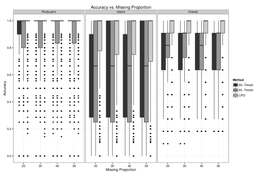
A constructed no-change pixel consists of whole years of data being sampled one year at a time from the portion of these 100 pixels identified as “background.” A constructed change pixel begins with a randomly generated change point configuration which partitions the time series into “background” and “change” periods; then data for these periods are sampled again, one year at a time, from the “background” and “change” portions of the 100 training pixels. A single replication involves simulating 60 no-change pixels and 60 change pixels. For each pixel we stitch together 11 years of data. Each annual profile consists of data for bands 1 through 7 over 19 time points, as described in Section 2. A single batch consists of 100 such replications. To explore the influence of missing data we created data for four batches, and induced minimum proportions of missing data of 20%, 30%, 40% and 50% in each batch respectively. As a basis for comparison, we applied our proposed change point method as well as another contemporary method (Huang and Friedl, 2014) to these simulated data.

Figure 3: Batch accuracies for three different methods applied to simulated change and no-change data using the metrics outlined in (11). The “90-Thresh” and “95-Thresh” correspond to the method in (Huang and Friedl, 2014) with thresholds of 90% and 95%; “CPD” corresponds to our proposed method.

Table 2: Average overall accuracies in each batch, for each of the three methods.

Missing %	90-Thresh	95-Thresh	CPD
20	0.781	0.794	0.920
30	0.782	0.796	0.916
40	0.780	0.793	0.913
50	0.779	0.792	0.909

To measure the performance of a change point method we consider three metrics: producer’s accuracy $P$ (sensitivity, recall), user’s accuracy $U$ (positive predictive value, precision), and (overall) accuracy $A$. Given two change point configurations $\rho$, as classified by the method, and $\widetilde{\rho}$, the ground truth configuration, each metric is given by:

$$\begin{split}P(\rho,\widetilde{\rho})&=\frac{\sum_{i=1}^{J}I(i\not\in\text{BG}(\rho))I(i\not\in\text{BG}(\widetilde{\rho}))}{\sum_{i=1}^{J}I(i\not\in\text{BG}(\widetilde{\rho}))},\\ U(\rho,\widetilde{\rho})&=\frac{\sum_{i=1}^{J}I(i\not\in\text{BG}(\rho))I(i\not\in\text{BG}(\widetilde{\rho}))}{\sum_{i=1}^{J}I(i\not\in\text{BG}(\rho))},~{}\text{and}\\ A(\rho,\widetilde{\rho})&=\frac{1}{J}\sum_{i=1}^{J}I(i\not\in\text{BG}(\rho))I(i\not\in\text{BG}(\widetilde{\rho}))+I(i\in\text{BG}(\rho))I(i\in\text{BG}(\widetilde{\rho})).\end{split}$$ (11)

If the denominator in either $P$ or $U$ is zero we arbitrarily set them to zero. The boxplots in Figure 3 and values in Table 2 summarize the three accuracies mentioned above for our proposed method as well as the method in (Huang and Friedl, 2014) with thresholds of 90% and 95%. In every situation our proposed method out-performs the contemporary method at both 90% and 95% thresholds. Furthermore, our method consistently achieves high accuracies ($>$90%) across substantial amounts of missing data. The noticeable dip in user’s accuracy (as compared with producer’s and overall) across all methods stems from a tendency to identify an excessively long change period. To adapt to this we could consider updating our belief about the probability of recovery. After successfully applying our method to simulated data, we proceed to detect change in a particular region of the Xingu River Basin.

3.2 Case Study

We apply the EM algorithm described in Section 2.2 to an area (2500 MODIS pixels, $\approx$134 $km^{2}$) in the Xingu River Basin, located in the Southeastern part of the Amazon in the State of Mato Grosso, Brazil. The study region has several distinct types of natural vegetation including moist tropical rainforest, cerrado, and deciduous forest. Despite containing substantial area of protected indigenous lands, large areas of the basin’s EBF have been converted to agricultural lands for soybean production and cattle ranching since 2000 (Huang and Friedl, 2014).

To avoid spurious results, we do not consider IGBP classes that are not native to the study area: 1 (evergreen needleleaf forests), 3 (deciduous needleleaf forests), and 4 (deciduous broadleaf forest), 11 (permanent wetlands), 13 (urban and built-up), and 15 (snow and ice). Thus, only IGBP classes 5 (MXF), 6 (CSH), 7 (OSH), 8 (WSA), 9 (SAV), 10 (GRA), 12 (CRL), 14 (CRM), 16 (BAR), and 17 (WAT) are assumed as possible change classes, while IGBP class 2, EBF, is taken as the background class. For the analysis we assumed that $\pi_{0}=10^{-10}$, $\pi_{R}=0.01$, and that $\kappa_{0}=\kappa_{c}=5\cdot 10^{4}$ which is roughly $1/5$ of the data variance in the classes. The very stringent value for the probability of change $\pi_{0}$ aims at providing a more robust change point inference against outliers. As the probability of recovery $\pi_{R}$ suggests, we expect that a priori approximately $1\%$ of the changed pixels actually recover.

To assess our results, we used a high quality Landsat-based deforestation dataset called PRODES (Monitoring the Brazilian Amazon Gross Deforestation), produced by Brazil’s National Institute for Space Research (INPE) (INPE, 2012). We derived annual sub-pixel fractions of deforestation and the year of change at MODIS spatial resolution (see (Huang and Friedl, 2014) for details). In particular, to evaluate the performance of our method, for each pixel $v\in\mathscr{R}$ we compare the estimated change segmentation given by $\rho_{v}$ to reference deforestation percentages $f_{v}$ using a measure of concordance $C$:

$$C(\rho_{v},f_{v}):=\frac{1}{J}\sum_{i=1}^{J}I(i\in\text{BG}(\rho_{v}))(1-f_{iv})+I(i\not\in\text{BG}(\rho_{v}))f_{iv}.$$ (12)

We note that this measure can be seen as an expected accuracy if we regard $f_{iv}$ as the probability of the $i$-th reference year not being in the background state.

Figure 4: Results of change point analysis in the Xingu River study region. Top row: estimated change points $\widehat{\rho}_{1v}$ in the leftmost panel (darker shades mean earlier changes), conditional probabilities of no change in the rightmost panels (darker shades represent smaller probabilities.) Bottom row, left to right: ground-truth reference (darker shades code for higher deforestation), concordance with estimated change point configurations (darker shades capture lower concordance), and distribution of concordance values across pixels.

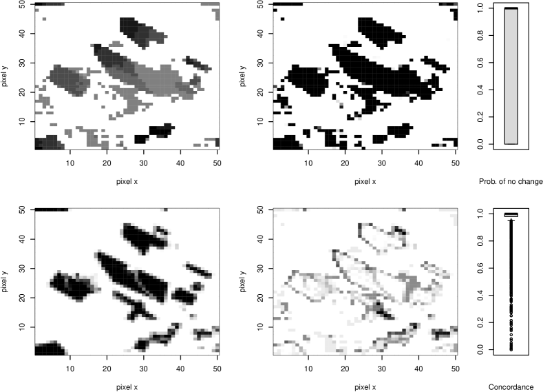
Figure 4 summarizes the inferred changes. In the top left panel we plot the estimated change year for each pixel $\widehat{\rho}_{1v}$ at the end of the EM procedure for pixel $v$. Darker grays represent earlier changes and white, in particular, codes for $\widehat{\rho}_{1v}=J$, i.e. no change. The two top rightmost panels show the conditional probability of no change, that is, ${\mathbb{P}}(\rho_{1v}=J{\,|\,}Y_{v};\widehat{\Theta})$, with darker shades representing smaller probabilities; as can be seen from the contrast in the spatial pattern and the boxplot, the changes are very accentuated within clusters. The bottom panels show that the inferred change points are in very good agreement with the ground-truth reference: the leftmost panel plots $\max_{i=1,\ldots,J}f_{iv}$, with darker shades representing higher levels of deforestation; the middle panel plots the concordance measure in (12), darker shades coding for lower concordance values to highlight contrasts; and the rightmost panel illustrating the distribution of concordance values across pixels. As we can see, concordance is overall high and the low values are concentrated either at the borders of change clusters or at small change “islands” (clusters.)

Figure 5: Results of change point analysis in the Xingu River study region. Top row: estimated change points, land cover class compositions (top panels), and projected profiles (bottom panels) for two representative pixels in the study region. In top panels: probability of first change point with change weights given in color according to land cover class (see legend), dashed line marks probability of no change, dark gray bar marks probability of second change to background class (recovery), light gray background represents deforestation percentages from ground-truth reference; in bottom panels: PC-projected spectro-temporal data profiles, with hollow points marking EM-imputed values, solid lines representing mean land cover profiles, and dashed lines mean profiles for background class. Bottom-left panel: probabilities of land cover changes (bars) given that change has occurred; jittered points highlight the same probabilities but when these probabilities are maximized for the respective change class. Bottom-right panel: overall land cover classification based on inferred change.

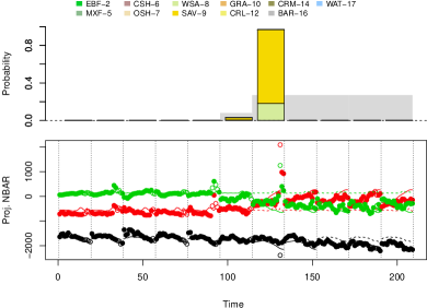
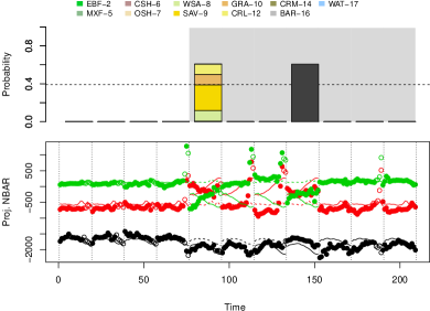
An important feature of our model is to not only represent changes but to also characterize these changes according to land cover classes. As an example, the top row of Figure 5 illustrates the results for two typical pixels in the study region. In each panel, the top plot shows the probability of change points, ${\mathbb{P}}(\rho_{1v}{\,|\,}Y_{v};\widehat{\Theta})$, further stratified by class probabilities ${\mathbb{P}}(W_{v}{\,|\,}Y_{v};\widehat{\Theta})$ in a colored bar, ${\mathbb{P}}(\rho_{2v}{\,|\,}Y_{v};\widehat{\Theta})$ in a dark gray bar if positive, and the deforestation percentages from the ground-truth reference in light gray in the background. The dashed line represents the probability of no change. The bottom plot depicts PC-projected NBAR values as in (2) with $K=3$ with EM-imputed values in hollow points; the solid lines in each year outline the projected mean profile for the inferred class in the year, while dashed lines represent background (EBF) yearly profiles. As we can see from the left panel, the changed class profile fits the data reasonably well, and hence the high probability of change at year 7; on the other hand, in the right panel the projected data does not seem to follow class profiles closely and so the no-change probability is closer to the now smaller change probability and the class to which the pixel changed is less certain.

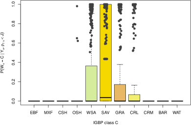
The bottom row portrays to which land cover classes pixels change (left panel, posterior conditional probabilities ${\mathbb{P}}(W_{v}{\,|\,}Y_{v},\rho_{1v}>J)$) and how these change classes are distributed spatially in the study region (right panel.) In the left barplot, we see that the most common change classes are, in order, savannas (IGBP class 9), woody savannas (IGBP 8), grasslands (IGBP 10), and croplands (IGBP 12.) The jittered gray points highlight the probability of changing to each class $C$ when ${\mathbb{P}}(W_{v}{\,|\,}Y_{v},\rho_{1v}>J)$ is maximized at $C$. The right panel displays the study region with each pixel colored by either the background EBF class if there is no inferred change, or by the class that maximizes ${\mathbb{P}}(W_{v}{\,|\,}Y_{v},\rho_{1v}>J)$ in case of change. Thus, the panel contains the same spatial patterns as in the top two leftmost panels in Figure 4, but it adds a characterization of change according to land cover.

4 Discussion

As the simulation study in Section 3.1 indicates, the proposed model and EM inferential routine yield better results than a state-of-the-art alternative method. Our better performance can be explained mainly by three factors: first, our proposed model incorporates data from all bands, instead of relying on particular bands or combined statistics (e.g. NDVI and EVI (Myneni et al., 1995; Huete et al., 2002)); missing data is ubiquitous in remote sensing and while many methods depend on extraneous gap-filling procedures, our method accommodates missing data consistently with our model via expectation; finally, our model is more flexible since we allow for at most two change points to capture recovery from change.

Our proposed methodology has also performed well in the real-world case study in Section 3.2. The results are in very good agreement with the ground-truth reference. Interestingly, as we can see in Figure 4, the inferred changes seem to follow a clear spatial pattern usually going northwest to southeast and operating on clusters; this effect is reassuring since the model makes no provisions for spatial interactions and so the pattern is fortuitous. Concordance is generally high over the whole study region with low concordance pixels being localized to change cluster borders—which we attribute to pixels with mixed class compositions due to transitions from background (see, for example, (Jin and Sader, 2005; Lunetta et al., 2006))—or to small clusters. These small clusters capture larger discrepancies with the reference about the existence of change and/or deforestation.

The two exemplar pixels in Figure 5 highlight the two major types of discrepancies to the ground-truth reference that lead to lower concordance values in Figure 4. In the top left panel we have a low deforestation percentage but high estimated probability of change at year 7 to savanna; this pixel belongs to the small cluster in the southeast corner of the region. Given that the spectro-temporal profile for savanna is similar to the profile for evergreen broadleaf forests (EBF, the background land cover class), and that savannas have from 10 to 30% of forest canopy cover, it is reasonable to confuse this land cover class with a low deforestation profile. In the top right panel we summarize the results from the EM method for a pixel in the southern border of the big change cluster in the middle of the study region. In this case, the class fragmentation at the change year, year 5, and possible recovery at year 8 can be attributed to deforestation and/or degradation at sub-pixel scale.

As we can see in the bottom left panel of Figure 5, in the Xingu River region case study most land cover classes in the estimated change segments are woody savannas, savannas, grasslands, or croplands (IGBP classes 8, 9, 10, and 12, respectively). Croplands and grasslands are often found in regions with earlier change points (darker regions in the top left plot in Figure 4), and might correspond to new land uses such as soy plantations and cattle ranching farms. In contrast, later change point regions are often classified as woody savannas, which have higher canopy density and might signal recent deforestation. Savannas have lower canopy density and are localized to either border pixels, as a transition land cover class, or to isolated islands; these smaller stranded regions could correspond to degradation areas, a more veiled form of deforestation. Interestingly, most discrepancies to the reference deforestation percentages overlap with this land cover class; this can be explained by lower deforestation percentages in these regions.

5 Conclusion

Detecting changes in land cover can provide crucial information for land use policy, natural resource management, and ecosystem modeling efforts. Remote sensing offers a spectrally and temporally rich source of data with which to make inference about changes in land cover at broad spatial scales. Unfortunately, missing values pervade most datasets for a multitude of reasons.

In this article we proposed a hierarchical model for identifying conversion-type changes in MODIS time series which accounts for missing data. The collection of MODIS training sites for the IGBP classification scheme is extensive and provides a useful resource for characterizing these high-dimensional data. We use these training data to estimate model parameters for 11 IGBP land cover classes including our background class: Evergreen Broadleaf Forest. With these estimates in hand we proceed to analyze pixels independently with an EM algorithm to detect the presence or lack of change points. The change points we identify characterize distributional changes from EBF to one of the other IGBP land cover classes present in our training dataset.

Not only can our approach identify change points, but the posteriors in (8) can be used to informally assess what class or classes the changed data represent. The methodology we propose here has two distinctive features: first, while our method is probably best used to find abrupt changes in time series, such as disturbances, it is flexible enough to handle gradual changes by suitably defining change probabilities $\pi_{0}$ and $\pi_{R}$ and fitting class probabilities $\alpha$; moreover, the methodology we propose allows for recovery from change. These two important features are essential to characterizing and interpreting changes and are, in particular, essential to remote sensing applications. We note that hyper-prior parameters $\pi_{0}$ and $\pi_{R}$ control how robust the method is to outliers and should be carefully elicited based on similar study regions.

In general, our EM algorithm could be used successfully on data or land cover displaying a conversion-type change. To accommodate other types of disturbances such fire and logging, our model would require exemplars from these situations. That is, we would need to characterize the surface after a fire or after logging in the parameter estimates of (1) (i.e. training data for “post-fire” or “post-logging”) in order to detect these kinds of changes in new pixels.

We demonstrated the effectiveness of our method with a simulation study and a case study in the Xingu River Basin. Our results indicate that our method performs better than state-of-the-art methods and has high concordance to ground-truth references. More specifically, we recovered nicely the spatial and temporal configuration of changes in the study regions and were able to interpret the changes by their inferred land cover classes and spatial localization. Overall, our method produced satisfying results and should be considered for detecting conversion-type changes in remotely sensed time series that contain missing data.

As future work we intend to extend this method to formally account for changes in space, that is, not only in time, and to investigate an alternative estimator for change configurations that maximizes the posterior expected accuracy, that is, to define $\widehat{\rho}_{A}:=\mathop{\rm arg\,max}\limits_{\widetilde{\rho}}{\mathbb{E}}_{\rho{\,|\,}Y}\big{[}A(\rho,\widetilde{\rho})\big{]}$ and devise a computationally efficient method to obtain $\widehat{\rho}_{A}$.

Appendix A Expectation-Maximization Derivations

To derive the EM updates in Section 2.2 we need

$$\begin{split}Q(\Theta,\Theta^{(t)})&={\mathbb{E}}_{Z,W{\,|\,}Y;\Theta^{(t)}}\Big{[}\log{\mathbb{P}}(\Theta,Z,W,Y)\Big{]}\\ &={\mathbb{E}}_{Z,W{\,|\,}Y;\Theta^{(t)}}\Bigg{[}\sum_{v\in\mathscr{R}}\log{\mathbb{P}}(Z_{v},Y_{v}{\,|\,}W_{v},\rho_{v})+\log{\mathbb{P}}(\rho_{v})\\ &\qquad+I(\rho_{1v}<J)\log{\mathbb{P}}(W_{v}{\,|\,}\boldsymbol{\alpha})+\log{\mathbb{P}}(\boldsymbol{\alpha})\Bigg{]},\end{split}$$

as defined in (6). The indicator $I(\rho_{1v}<J)$ filters pixels that have at least one change. To derive the conditional updates for $\boldsymbol{\alpha}$ and $\rho_{v}$ for each $v\in\mathscr{R}$ we identify two functions that capture the terms in $Q$ that depend on $\boldsymbol{\alpha}$,

$$\begin{split}Q_{\alpha}(\Theta,\Theta^{(t)})&={\mathbb{E}}_{Z,W{\,|\,}Y;\Theta^{(t)}}\Bigg{[}\sum_{v:\rho_{1v}<J}\log{\mathbb{P}}(W_{v}{\,|\,}\boldsymbol{\alpha})+\log{\mathbb{P}}(\boldsymbol{\alpha})\Bigg{]}\\ &=\sum_{v:\rho_{1v}<J}{\mathbb{E}}_{W_{v}{\,|\,}Y_{v};\Theta^{(t)}}\Big{[}\log{\mathbb{P}}(W_{v}{\,|\,}\boldsymbol{\alpha})\Big{]}+\log{\mathbb{P}}(\boldsymbol{\alpha}),\end{split}$$ (13)

and on $\rho_{v}$ at pixel $v$,

$$\begin{split}Q_{\rho,v}(\Theta,\Theta^{(t)})&={\mathbb{E}}_{Z_{v},W_{v}{\,|\,}Y_{v};\Theta_{v}^{(t)}}\Big{[}\log{\mathbb{P}}(Z_{v},Y_{v}{\,|\,}W_{v},\rho_{v})+\log{\mathbb{P}}(\rho_{v})\\ &\qquad+I(\rho_{1v}<J)\log{\mathbb{P}}(W_{v}{\,|\,}\boldsymbol{\alpha})\Big{]}\\ &={\mathbb{E}}_{Z_{v},W_{v}{\,|\,}Y_{v};\Theta_{v}^{(t)}}[\log{\mathbb{P}}(Z_{v},Y_{v}{\,|\,}W_{v},\rho_{v})]+\log{\mathbb{P}}(\rho_{v})\\ &\qquad+I(\rho_{1v}<J){\mathbb{E}}_{Z_{v},W_{v}{\,|\,}Y_{v};\Theta_{v}^{(t)}}[\log{\mathbb{P}}(W_{v}{\,|\,}\boldsymbol{\alpha})].\\ \end{split}$$ (14)

Note that $Q(\Theta,\Theta^{(t)})=\sum_{v}Q_{\rho,v}(\Theta,\Theta^{(t)})+\log{\mathbb{P}}(\boldsymbol{\alpha})$ and that the term $I(\rho_{1v}<J){\mathbb{P}}(W_{v}{\,|\,}\boldsymbol{\alpha})$ is shared between $Q_{\alpha}$ and $Q_{\rho,v}$.

Updating $\boldsymbol{\alpha}$

Let us start with the $\boldsymbol{\alpha}$-update in Step 2.a; we need to optimize $Q$ with respect to $\boldsymbol{\alpha}$ subject to the constraint $h(\boldsymbol{\alpha})=\sum_{g\in\mathscr{C}}\alpha_{g}-1=0$. To this end, we define a Lagrange multiplier $\lambda$ and solve

$$\frac{\partial}{\partial\alpha_{k}}\Big{[}Q_{\alpha}(\Theta,\Theta^{(t)})-\lambda h(\boldsymbol{\alpha})\Big{]}=\frac{\partial}{\partial\alpha_{k}}\Bigg{[}\sum_{v:\rho_{1v}<J}{\mathbb{E}}_{W_{v}{\,|\,}Y_{v};\Theta^{(t)}}\Bigg{[}\sum_{g\in\mathscr{C}}I(W_{v}=g)\log\alpha_{g}\Bigg{]}\\ +\sum_{g\in\mathscr{C}}(\pi_{g}-1)\log\alpha_{g}-\lambda\sum_{g\in\mathscr{C}}\alpha_{g}\Bigg{]}=0,$$

and so, fixing $\rho_{v}$ to its value in the previous iteration, $\rho_{v}^{(t)}$, we get the update in (7),

$$\begin{split}\alpha_{k}^{(t+1)}&=\frac{\pi_{k}-1+\sum_{v:\rho_{1v}^{(t)}<J}{\mathbb{E}}_{W_{v}{\,|\,}Y_{v};\Theta^{(t)}}[I(W_{v}=k)]}{\lambda}\\ &=\frac{\sum_{v:\rho_{1v}^{(t)}<J}{\mathbb{P}}(W_{v}=k{\,|\,}Y_{v};\Theta^{(t)})+\pi_{k}-1}{\sum_{g\in\mathscr{C}}\big{[}\sum_{v:\rho_{1v}^{(t)}<J}{\mathbb{P}}(W_{v}=g{\,|\,}Y_{v};\Theta^{(t)})+\pi_{g}-1\big{]}}\\ &=\frac{\sum_{v:\rho_{1v}^{(t)}<J}{\mathbb{P}}(W_{v}=k{\,|\,}Y_{v};\Theta^{(t)})+\pi_{k}-1}{N_{v}^{(t)}+\sum_{g\in\mathscr{C}}\pi_{g}-|\mathscr{C}|},\end{split}$$

where $N_{v}^{(t)}=\sum_{v:\rho_{1v}^{(t)}<J}\sum_{g\in\mathscr{C}}{\mathbb{P}}(W_{v}=g{\,|\,}Y_{v};\Theta^{(t)})=\sum_{v:\rho_{1v}^{(t)}<J}1$ is the number of pixels with changes. To compute the update we just need the expression in (8), for $k\in\mathscr{C}$,

$$\begin{split}{\mathbb{P}}(W_{v}=k{\,|\,}Y_{v};\Theta^{(t)})&=\frac{{\mathbb{P}}(Y_{v}{\,|\,}W_{v}=k;\Theta^{(t)}){\mathbb{P}}(W_{v}=k;\Theta^{(t)})}{\sum_{g\in\mathscr{C}}{\mathbb{P}}(Y_{v}{\,|\,}W_{v}=g;\Theta^{(t)}){\mathbb{P}}(W_{v}=g;\Theta^{(t)})}\\ &=\frac{\alpha_{k}^{(t)}{\mathbb{P}}(Y_{v}{\,|\,}W_{v}=k;\Theta^{(t)})}{\sum_{g\in\mathscr{C}}\alpha_{g}^{(t)}{\mathbb{P}}(Y_{v}{\,|\,}W_{v}=g;\Theta^{(t)})}.\end{split}$$

Updating $\rho_{v}$

In Step 2.b we fix $\boldsymbol{\alpha}$ and update the remaining parameters in $\Theta$. We update them jointly, but in parallel for each pixel. The last term in $Q_{\rho,v}$ is already known from the last section, and we condition $\boldsymbol{\alpha}$ to its recently updated value $\boldsymbol{\alpha}^{(t+1)}$:

$${\mathbb{E}}_{Z_{v},W_{v}{\,|\,}Y_{v};\Theta_{v}^{(t)}}\Big{[}\log{\mathbb{P}}(W_{v}{\,|\,}\boldsymbol{\alpha})\Big{]}=\sum_{g\in\mathscr{C}}{\mathbb{P}}(W_{v}=g{\,|\,}Y_{v};\Theta^{(t)})\log\alpha_{g}^{(t+1)}.$$ (15)

Now we just need to obtain

$${\mathbb{E}}_{Z_{v},W_{v}{\,|\,}Y_{v};\Theta_{v}^{(t)}}\Big{[}\log{\mathbb{P}}(X_{v}{\,|\,}W_{v},\rho_{v})\Big{]}={\mathbb{E}}_{W_{v}{\,|\,}Y_{v};\Theta_{v}^{(t)}}\Bigg{[}\sum_{g\in\mathscr{C}}I(W_{v}=g)\\ {\mathbb{E}}_{Z_{v}{\,|\,}W_{v}=g,Y_{v};\Theta_{v}^{(t)}}\Big{[}\log{\mathbb{P}}(X_{v}{\,|\,}W_{v},\rho_{v})\Big{]}\Bigg{]}\\ =-\frac{1}{2}\Bigg{(}\sum_{i\in\text{BG}(\rho_{v})}S(X_{iv};\mu_{F},\widetilde{\Sigma}_{F})+\sum_{i\not\in\text{BG}(\rho_{v})}\sum_{g\in\mathscr{C}}{\mathbb{P}}(W_{v}=g{\,|\,}Y_{v};\Theta^{(t)})S(X_{iv};\mu_{g},\widetilde{\Sigma}_{g})\Bigg{)},$$ (16)

where $\widetilde{\Sigma}_{F}=\Sigma_{F}+\kappa_{0}I_{BT}$, $\widetilde{\Sigma}_{g}=\Sigma_{g}+\kappa_{c}I_{BT}$ for $g\in\mathscr{C}$, as in the main text, and, if $X\sim N(\mu,\Sigma)$ with missing entries at indices miss,

$$S(X;\mu,\Sigma):=\log|\Sigma|+{\mathbb{E}}_{X_{{\text{\sf miss}}}{\,|\,}X_{-{\text{\sf miss}}}}\Big{[}{(X-\mu)}^{\top}\Sigma^{-1}(X-\mu)\Big{]}.$$

To evaluate $S$, we need

$$\begin{split}{\mathbb{E}}_{X_{{\text{\sf miss}}}{\,|\,}X_{-{\text{\sf miss}}}}\Big{[}{(X-\mu)}^{\top}\Sigma^{-1}(X-\mu)\Big{]}&={\mathbb{E}}_{X_{{\text{\sf miss}}}{\,|\,}X_{-{\text{\sf miss}}}}\Big{[}\text{tr}\Big{\{}{(X-\mu)}^{\top}\Sigma^{-1}(X-\mu)\Big{\}}\Big{]}\\ &=\text{tr}\Big{\{}\Sigma^{-1}{\mathbb{E}}_{X_{{\text{\sf miss}}}{\,|\,}X_{-{\text{\sf miss}}}}\Big{[}(X-\mu){(X-\mu)}^{\top}\Big{]}\Big{\}}\\ &={(\widetilde{X}-\mu)}^{\top}\Sigma^{-1}(\widetilde{X}-\mu)\\ &\qquad+\text{tr}\Big{\{}\Sigma^{-1}{\text{\sf Var}}_{X_{{\text{\sf miss}}}{\,|\,}X_{-{\text{\sf miss}}}}[X]\Big{\}},\end{split}$$

since, with $\widetilde{X}={\mathbb{E}}_{X_{{\text{\sf miss}}}{\,|\,}X_{-{\text{\sf miss}}}}[X]$, we have the Pythagorean relationship

$$\begin{split}{\mathbb{E}}_{X_{{\text{\sf miss}}}{\,|\,}X_{-{\text{\sf miss}}}}\Big{[}(X-\mu){(X-\mu)}^{\top}\Big{]}&={\mathbb{E}}_{X_{{\text{\sf miss}}}{\,|\,}X_{-{\text{\sf miss}}}}\Big{[}(X-\widetilde{X}){(X-\widetilde{X})}^{\top}\\ &\qquad+(\widetilde{X}-\mu){(\widetilde{X}-\mu)}^{\top}\Big{]}\\ &={\text{\sf Var}}_{X_{{\text{\sf miss}}}{\,|\,}X_{-{\text{\sf miss}}}}[X]+(\widetilde{X}-\mu){(\widetilde{X}-\mu)}^{\top}.\end{split}$$

Let us denote by $V(X;\Sigma):={\text{\sf Var}}_{X_{{\text{\sf miss}}}{\,|\,}X_{-{\text{\sf miss}}}}[X]$. Clearly, $\widetilde{X}_{-{\text{\sf miss}}}=X_{-{\text{\sf miss}}}$ and so ${V(X;\Sigma)}_{jk}=0$ wherever $j\not\in{\text{\sf miss}}$ or $k\not\in{\text{\sf miss}}$. The remaining entries in $\widetilde{X}$ and $V(X;\Sigma)$ are known from

$$X_{{\text{\sf miss}}}{\,|\,}X_{-{\text{\sf miss}}}\sim N\Big{(}\mu_{{\text{\sf miss}}}+{(\Sigma_{-{\text{\sf miss}},{\text{\sf miss}}})}^{\top}{(\Sigma_{-{\text{\sf miss}},-{\text{\sf miss}}})}^{-1}(X_{-{\text{\sf miss}}}-\mu_{-{\text{\sf miss}}}),\\ \Sigma_{{\text{\sf miss}},{\text{\sf miss}}}-{(\Sigma_{-{\text{\sf miss}},{\text{\sf miss}}})}^{\top}{(\Sigma_{-{\text{\sf miss}},-{\text{\sf miss}}})}^{-1}\Sigma_{-{\text{\sf miss}},{\text{\sf miss}}}\Big{)}.$$

Thus,

$$S(X;\mu,\Sigma)=\log|\Sigma|+{(\widetilde{X}-\mu)}^{\top}\Sigma^{-1}(\widetilde{X}-\mu)+\sum_{j,k\in{\text{\sf miss}}}{(\Sigma^{-1})}_{jk}{V(X;\Sigma)}_{jk},$$

which yields the definition in (10).

Finally, putting together (15) and (16) in the definition of $Q_{\rho,v}$, and since $\mathop{\rm arg\,max}\limits_{\rho}Q_{\rho,v}=\mathop{\rm arg\,min}\limits_{\rho}-2Q_{\rho,v}$, we have the update expression in (9).

References

- Basseville and Nikiforov (1993) Basseville, M. and I. V. Nikiforov (1993). Detection of Abrupt Changes: Theory and Application. Prentice-Hall, Inc.
- Bonan et al. (2002) Bonan, G. B., K. W. Oleson, M. Vertenstein, S. Levis, X. Zeng, Y. Dai, R. E. Dickinson, and Z.-L. Yang (2002). The land surface climatology of the community land model coupled to the NCAR community climate model. Journal of Climate 15(22), 3123–3149.
- Booth and Smith (1982) Booth, N. B. and A. F. M. Smith (1982). A Bayesian approach to retrospective identification of change-points. Journal of Econometrics 19(1), 7–22.
- Boriah (2010) Boriah, S. (2010). Time series change detection: Algorithms for land cover change. Ph. D. thesis, University of Minnesota.
- Carlin and Louis (2000) Carlin, B. P. and T. A. Louis (2000). Bayes and empirical Bayes methods for data analysis (Second ed.). New York, USA: Chapman and Hall/CRC.
- Chu and Zhao (2004) Chu, P.-S. and X. Zhao (2004). Bayesian Change-Point Analysis of Tropical Cyclone Activity: The Central North Pacific Case. Journal of Climate 17(24), 4893–4901.
- Coops et al. (2009) Coops, N. C., M. A. Wulder, and D. Iwanicka (2009). Large area monitoring with a MODIS-based Disturbance Index (DI) sensitive to annual and seasonal variations. Remote Sensing of Environment 113(6), 1250–1261.
- Coppin et al. (2004) Coppin, P., I. Jonckheere, K. Nackaerts, B. Muys, and E. Lambin (2004). Digital change detection methods in ecosystem monitoring: a review. International Journal of Remote Sensing 25(9), 1565–1596.
- Davis and Holmgren (2000) Davis, R. and P. Holmgren (2000). Fra 2000: Forest cover mapping & monitoring with noaa-avhrr & other coarse spatial resolution sensors. Forest Resources Assessment Programme.
- Dawid (1981) Dawid, A. (1981). Some matrix-variate distribution theory: notational considerations and a bayesian application. Biometrika 68(1), 265–274.
- Dempster et al. (1977) Dempster, A. P., N. M. Laird, and D. B. Rubin (1977). Maximum likelihood from incomplete data via the EM algorithm. Journal of the Royal statistical Society 39(1), 1–38.
- Ek et al. (2003) Ek, M., K. Mitchell, Y. Lin, E. Rogers, P. Grunmann, V. Koren, G. Gayno, and J. Tarpley (2003). Implementation of Noah land surface model advances in the National Centers for Environmental Prediction operational mesoscale Eta model. Journal of Geophysical Research 108(D22), 8851.
- Ellis and Ramankutty (2008) Ellis, E. C. and N. Ramankutty (2008). Putting people in the map: anthropogenic biomes of the world. Frontiers in Ecology and the Environment 6(8), 439–447.
- Elsner et al. (2000) Elsner, J. B., T. Jagger, and X. Niu (2000). Changes in the rates of North Atlantic major hurricane activity during the 20th century. Geophysical Research Letters 27(12), 1743–1746.
- Fearnhead (2006) Fearnhead, P. (2006). Exact and Efficient Bayesian Inference for Multiple Change Point Problems. Statistics and computing.
- Fearnhead and Liu (2007) Fearnhead, P. and Z. Liu (2007). On-line inference for multiple changepoint problems. Journal of the Royal Statistical Society: Series B (Statistical Methodology) 69(4), 589–605.
- Foley et al. (2005) Foley, J., R. DeFries, G. Asner, C. Barford, G. Bonan, S. Carpenter, F. Chapin, M. Coe, G. Daily, H. Gibbs, J. Helkowski, T. Holloway, E. Howard, C. Kucharik, C. Monfreda, J. Patz, I. Prentice, N. Ramankutty, and P. Snyder (2005). Global consequences of land use. Science 309(5734), 570–574.
- Friedl et al. (2010) Friedl, M. A., D. Sulla-Menashe, B. Tan, A. Schneider, N. Ramankutty, A. Sibley, and X. Huang (2010). MODIS Collection 5 global land cover: Algorithm refinements and characterization of new datasets. Remote Sensing of Environment 114(1), 168–182.
- Galeano and Peña (2007) Galeano, P. and D. Peña (2007, jan). Covariance changes detection in multivariate time series. Journal of Statistical Planning and Inference 137(1), 194–211.
- Gelman et al. (2003) Gelman, A., J. B. Carlin, H. S. Stern, and D. B. Rubin (2003). Bayesian data analysis (Second ed.). New York, USA: Chapman and Hall/CRC.
- Glanz et al. (2014) Glanz, H., L. Carvalho, D. Sulla-Menashe, and M. A. Friedl (2014). A parametric model for classifying land cover and evaluating training data based on multi-temporal remote sensing data. ISPRS Journal of Photogrammetry and Remote Sensing 97(0), 219–228.
- Goldewijk (2001) Goldewijk, K. K. (2001). Estimating global land use change over the past 300 years: the hyde database. Global Biogeochemical Cycles 15(2), 417–433.
- Gombay (2008) Gombay, E. (2008, mar). Change detection in autoregressive time series. Journal of Multivariate Analysis 99(3), 451–464.
- Honaker and King (2010) Honaker, J. and G. King (2010). What to do about missing values in time-series cross-section data. American Journal of Political Science 54(2), 561–581.
- Huang et al. (2002) Huang, C., J. R. G. Townshend, S. Liang, S. Kalluri, and R. S. DeFries (2002). Impact of sensor’s point spread function on land cover characterization: assessment and deconvolution. Remote Sensing of Environment 80(2), 203–212.
- Huang and Friedl (2014) Huang, X. and M. A. Friedl (2014, jun). Distance Metric-Based Forest Cover Change Detection Using MODIS Time Series. International Journal Of Applied Earth Observation And Geoinformation 29, 78–92.
- Huete et al. (2002) Huete, A., K. Didan, T. Miura, E. P. Rodriguez, X. Gao, and L. G. Ferreira (2002). Overview of the radiometric and biophysical performance of the MODIS vegetation indices. Remote Sensing of Environment 83(1), 195–213.
- INPE (2012) INPE (2012). Project PRODES: Monitoring the Brazilian Amazon Forests by Satellite. Available at: http://www.dpi.inpe.br/prodesdigital/.
- Jerez et al. (2010) Jerez, J. M., I. Molina, P. J. Garcia-Laencina, E. Alba, N. Ribelles, M. Martin, and L. Franco (2010). Missing data imputation using statistical and machine learning methods in a real breast cancer problem. Artificial Intelligence in Medicine 50(2), 105–115.
- Jin and Sader (2005) Jin, S. and S. A. Sader (2005). MODIS time-series imagery for forest disturbance detection and quantification of patch size effects. Remote Sensing of Environment 99(4), 462–470.
- Junninen et al. (2004) Junninen, H., H. Niska, K. Tuppurainen, J. Ruuskanen, and M. Kolehmainen (2004). Methods for imputation of missing values in air quality data sets. Atmospheric Environment 38(18), 2895–2907.
- Lee (2010) Lee, T.-S. (2010, dec). Change-Point Problems: Bibliography and Review. Journal of Statistical Theory and Practice 4(4), 643–662.
- Linderman et al. (2005) Linderman, M., P. Rowhani, D. Benz, S. Serneels, and E. F. Lambin (2005). Land-cover change and vegetation dynamics across Africa. Journal of Geophysical Research-Atmospheres 110(D12).
- Little and Rubin (2002) Little, R. J. and D. B. Rubin (2002). Statistical Analysis with Missing Data. Wiley Interscience.
- Lu et al. (2004) Lu, D., P. Mausel, E. Brondizio, and E. Moran (2004). Change detection techniques. International Journal of Remote Sensing 25(12), 2365–2407.
- Lund and Reeves (2002) Lund, R. and J. Reeves (2002). Detection of undocumented changepoints: A revision of the two-phase regression model. Journal of Climate 15(17), 2547–2554.
- Lunetta et al. (1999) Lunetta, R. S., C. D. Elvidge, et al. (1999). Remote Sensing Change Detection: Environmental Monitoring Methods and Applications. Taylor & Francis Ltd.
- Lunetta et al. (2006) Lunetta, R. S., J. F. Knight, J. Ediriwickrema, J. G. Lyon, and L. D. Worthy (2006). Land-cover change detection using multi-temporal modis ndvi data. Remote Sensing of Environment 105(2), 142–154.
- Meng and Rubin (1993) Meng, X.-L. and D. B. Rubin (1993). Maximum likelihood estimation via the ECM algorithm: A general framework. Biometrika 80(2), 267–278.
- Menzefricke (1981) Menzefricke, U. (1981). A Bayesian analysis of a change in the precision of a sequence of independent normal random variables at an unknown time point. Applied Statistics 30(2), 141–146.
- Mildrexler et al. (2009) Mildrexler, D., M. Zhao, and S. Running (2009). Testing a MODIS global disturbance index across North America. Remote Sensing of Environment 113(10), 2103–2117.
- Myneni et al. (1995) Myneni, R. B., F. G. Hall, P. J. Sellers, and A. L. Marshak (1995). The interpretation of spectral vegetation indexes. Geoscience and Remote Sensing, IEEE Transactions on 33(2), 481–486.
- Ning and Cheng (2012) Ning, J. and P. E. Cheng (2012). A comparison study of nonparametric imputation methods. Statistics and Computing 22(1), 273–285.
- Perreault et al. (2000) Perreault, L., J. Bernier, B. Bobée, and E. Parent (2000, aug). Bayesian change-point analysis in hydrometeorological time series. Part 1. The normal model revisited. Journal of Hydrology 235(3-4), 221–241.
- Rahman et al. (2013) Rahman, A. F., D. Dragoni, K. Didan, A. Barreto-Munoz, and J. A. Hutabarat (2013). Detecting Large Scale Conversion of Mangroves to Aquaculture with Change Point and Mixed-Pixel Analyses of High-Fidelity MODIS Data. Remote Sensing of Environment 130, 96–107.
- Ramankutty and Foley (1999) Ramankutty, N. and J. A. Foley (1999). Estimating historical changes in global land cover: Croplands from 1700 to 1992. Global Biogeochemical Cycles 13(4), 997–1027.
- Robert and Casella (1999) Robert, C. and G. Casella (1999). Monte Carlo Statistical Methods. Springer New York.
- Rodionov (2005) Rodionov, S. N. (2005). A brief overview of the regime shift detection methods. In V. Velikova and N. Chipev (Eds.), Large-Scale Disturbances (Regime Shifts) and Recovery in Aquatic Ecosystems: Challenges for Management Toward Sustainability, UNESCO-ROSTE/BAS Workshop on Regime Shifts, pp. 17–24. UNESCO-ROSTE/BAS Workshop on Regime Shifts, 14-16 June 2005, Varna, Bulgaria, 17-24.
- Rogan et al. (2002) Rogan, J., J. Franklin, and D. A. Roberts (2002). A comparison of methods for monitoring multitemporal vegetation change using thematic mapper imagery. Remote Sensing of Environment 80(1), 143–156.
- Roy (2000) Roy, D. P. (2000). The impact of misregistration upon composited wide field of view satellite data and implications for change detection. IEEE Transactions on Geoscience and Remote Sensing 38(4), 2017–2032.
- Running and Coughlan (1988) Running, S. W. and J. C. Coughlan (1988). A general model of forest ecosystem processes for regional applications I. Hydrologic balance, canopy gas exchange and primary production processes. Ecological Modelling 42(2), 125–154.
- Sanderson et al. (2002) Sanderson, E., M. Jaiteh, M. Levy, K. Redford, A. Wannebo, and G. Woolmer (2002). The human footprint and the last of the wild. Bioscience 52(10), 891–904.
- Schaaf et al. (2002) Schaaf, C., F. Gao, A. Strahler, W. Lucht, X. Li, T. Tsang, N. Strugnell, X. Zhang, Y. Jin, J. Muller, P. Lewis, M. Barnsley, P. Hobson, M. Disney, G. Roberts, M. Dunderdale, C. Doll, R. d’Entremont, B. Hu, S. Liang, J. Privette, and D. P. Roy (2002). First operational BRDF, albedo nadir reflectance products from MODIS. Remote Sensing of Environment 83(1-2), 135–148.
- Shao and Zhang (2010) Shao, X. and X. Zhang (2010, sep). Testing for Change Points in Time Series. Journal Of The American Statistical Association 105(491), 1228–1240.
- Singh (1989) Singh, A. (1989). Digital change detection techniques using remotely-sensed data. International Journal of Remote Sensing 10(6), 989–1003.
- Solow and Beet (2005) Solow, A. R. and A. R. Beet (2005). A test for a regime shift. Fisheries Oceanography 14(3), 236–240.
- Song et al. (2007) Song, X., M. Wu, C. Jermaine, and S. Ranka (2007). Statistical change detection for multi-dimensional data. In Proceedings of the 13th ACM SIGKDD international conference on Knowledge discovery and data mining, pp. 667–676. ACM.
- Stephens (1994) Stephens, D. A. (1994). Bayesian retrospective multiple-changepoint identification. Journal of the Royal Statistical Society. Series C (Applied Statistics) 43(1), 159–178.
- Sterling and Ducharne (2008) Sterling, S. and A. Ducharne (2008). Comprehensive data set of global land cover change for land surface model applications. Global Biogeochemical Cycles 22(3).
- Sulla-Menashe et al. (2013) Sulla-Menashe, D., R. E. Kennedy, Z. Yang, J. Braaten, O. N. Krankina, and M. A. Friedl (2013). Detecting forest disturbance in the Pacific Northwest from MODIS time series using temporal segmentation. Remote Sensing of Environment 151, 114–123.
- Survey (2013) Survey, U. S. G. (2013). MODIS overview. https://lpdaac.usgs.gov/products/modis_overview.
- Tan et al. (2006) Tan, B., C. E. Woodcock, J. Hu, P. Zhang, M. Ozdogan, D. Huang, W. Yang, Y. Knyazikhin, and R. B. Myneni (2006). The impact of gridding artifacts on the local spatial properties of MODIS data: Implications for validation, compositing, and band-to-band registration across resolutions. Remote Sensing of Environment 105(2), 98–114.
- Tsay (1988) Tsay, R. S. (1988). Outliers, level shifts, and variance changes in time series. Journal of forecasting 7(1), 1–20.
- Verbesselt et al. (2010) Verbesselt, J., R. Hyndman, G. Newnham, and D. Culvenor (2010). Detecting trend and seasonal changes in satellite image time series. Remote Sensing of Environment 114(1), 106–115.
- Vitousek et al. (1997) Vitousek, P., H. Mooney, J. Lubchenco, and J. Melillo (1997). Human domination of Earth’s ecosystems. Science 277(5325), 494–499.
- Zhang (2012) Zhang, S. (2012). Nearest neighbor selection for iteratively knn imputation. Journal of Systems and Software 85(11), 2541–2552.