Impact of membrane bistability on dynamical response of neuronal populations

Abstract

Neurons in many brain areas can develop pronounced depolarized state of membrane potential (up state) in addition to the normal hyperpolarized down state near the resting potential. The influence of the up state on signal encoding, however, is not well investigated. Here we construct a one-dimensional bistable neuron model and calculate the linear response to noisy oscillatory inputs analytically. We find that with the appearance of an up state, the transmission function is enhanced by the emergence of a local maximum at some optimal frequency and the phase lag relative to the input signal is reduced. We characterize the dependence of the enhancement of frequency response on intrinsic dynamics and on the occupancy of the up state.

Introduction- Elevated state of neuronal membrane potential (MP), the so called up state, has been observed extensively in different brain areas exp . In this regime the MPs of neurons are characterized by a bimodal distribution resulting from two stable fixed points in membrane dynamics. This bistability of neuronal dynamics leads to synchronous transitions between the down and up states of neurons in a network and the development of global up and down states parga ; compte . The exact role of the bistability of membrane potential in signal encoding and processing is still not well understood.

Individual neurons in a network receive noisy synaptic inputs and fire spikes irregularly shadlen . Besides the stationary firing rate, one important characteristic of neuronal dynamics is the response to time varying signals superimposed on background noise knight . This dynamical response of cortical neurons has recently been measured experimentally up to 1 kHz of signal frequency, which revealed very hight cutoff frequencies kondgen . Theoretically, the linear response has been obtained analytically for the leaky integrate-and-fire (LIF) neuron brunel , in which membrane dynamics has only one stable fixed point, and for the $r-\tau$ model (a piecewise linear version of experiential integrate-and-fire model) wei , in which an additional unstable fixed point for action potential initiation was included. The effect of the unstable fixed point in membrane dynamics on dynamical response was also investigated numerically in other one-dimensional models and conductance-based models num . Theoretical characterization of dynamical response of neurons that exhibit up and down states, however, is still missing. Intuitively, when the membrane potential of a neuron has a higher probability to be around some depolarized voltage, it is more likely that a small oscillatory signal can contribute to the firing of spikes, leading to enhancement of frequency response. Here we propose an analytically solvable bistable neuron model to investigate the impact of the up state on the dynamical response of neurons.

Model description- In this work we construct a one-dimensional bistable neuron model, which has piecewise linear subthreshold dynamics and is analytically solvable for the linear response. The dynamics is described by the following Langevin equation,

$$\tau\dot{v} = f(v)+\mu+\sigma\eta(t)\;,$$ (1)

where

$$f(v) = \left\{\begin{aligned} &-v\;,\;\qquad-\infty<v\leq v_{0}\\ &r_{1}(v-v_{t1})\;,\;v_{0}<v\leq v_{1}\\ &r(v-v_{t0})\;,\;\;v_{1}<v\leq v_{b}\end{aligned}\right.$$ (2)

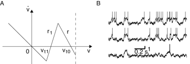
Here $v$ is the MP relative to the resting potential, $\mu$ is the mean external input, $\eta(t)$ is a Gaussian white noise which satisfies $\langle\eta(t)\rangle=0$ and $\langle\eta(t)\eta(t^{{}^{\prime}})\rangle=\tau\delta(t-t^{{}^{\prime}})$, and $\sigma$ is the strength of the noise. $\tau$ is the membrane time constant near the resting potential, which we will take as the unit of time in the theoretical result. Note that the membrane dynamics here might result from an interaction between patterned synaptic inputs and intrinsic membrane dynamics. Fig. 1A shows an illustration of the model dynamics when there is no external input. The slopes of the middle and right pieces are denoted as $r_{1}$ and $r$, respectively. Note that $r$ characterizes the membrane dynamics around the higher stable fixed point where the time constant is given by $\tau/|r|$. MPs at the crossing points of the left piece with the middle piece, and the middle piece with the right piece are denoted as $v_{0}$ and $v_{1}$, respectively. When there is no external input, $v_{t1}$ and $v_{t0}$ are the unstable fixed point and the higher stable fixed point, respectively. We will fix $v_{0}$ and $v_{t0}$, whereas $v_{t1}$ and $v_{1}$ are given by $v_{t1}=(1+1/r_{1})v_{0}$ and $v_{1}=(r_{1}v_{t1}-rv_{t0})/(r_{1}-r)$. The deterministic dynamics ($\sigma=0$ in Eq. (1)) possess one lower stable fixed point, one unstable fixed point and one higher stable fixed point, located at $v=\mu,\;v_{t1}-\mu/r_{1}\;\textrm{and}\;v_{t0}-\mu/r$, respectively. When the MP reaches an absorbing boundary $v_{b}$, it is reset to a resetting potential $v_{r}$ for a refractory period $\tau_{r}$. The larger one between $|\tilde{v}_{0}|$ and $|\tilde{v}_{b}|$ determines the rheobase current of the model neuron, where $\tilde{v}_{0}\equiv-v_{0}$ and $\tilde{v}_{b}\equiv r(v_{b}-v_{t0})$. Since the model neuron will never fire spikes when $|r|$ is very large if $v_{b}$ is fixed, we will fix $\tilde{v}_{b}$ and choose $v_{b}$ determined by $v_{b}=v_{t0}+\tilde{v}_{b}/r$. The relative values of $\tilde{v}_{0}$ and $\tilde{v}_{b}$ might indicate different dynamical regime of the model neuron. For example, a larger $|\tilde{v}_{b}|$ implies that the neuron can make a transition from the up-down regime to a tonically depolarized state when $\mu>|\tilde{v}_{0}|$, which is reminiscent to that observed for cortical neurons from sleep to wakefulness steriade . We are most interested in the noise-driven regime, i.e., the mean external current is smaller than the rheobase current, since real neurons work in a regime in which excitatory and inhibitory synaptic inputs to individual neurons balance each other somp . In this dynamic regime, our neuron model describes barrier penetration in a double well with reinjection of probability current after reaching an absorbing boundary. Here we focus on the case when $v_{r}$ is located within the middle piece, therefore the model neuron could fire several spikes before transiting to the down state, as normally observed for neurons exhibiting up state. Fig. 1B shows the MP trajectories for three different $r_{1}$. We see that with a larger $r_{1}$, the MP spends more times in the up state.

Figure 1: Illustration of the model. A, illustration of the piecewise linear model; B, MP trajectories for $r_{1}=1,5\;\textrm{and}\;10$ from bottom to top. Parameters used are: $r=-1,\;v_{0}=0.5,\;v_{r}=v_{t1},\;v_{t0}=2,\;\tilde{v}_{b}=-0.2,\;\tau=10\;\textrm{ms},\;\tau_{r}=0\;\textrm{ms},\;\mu=0,\;\sigma=0.5$.

The Fokker-Planck equation (FPE) framework- The FPE corresponding to Eq. (1) has the following form risken ,

$$\partial_{t}{P}(v,t)+\partial_{v}(f(v)+\mu-D\partial_{v})P(v,t)=0\;,$$ (3)

where $D=\frac{1}{2}\sigma^{2}$ is the diffusion constant. We will use both $D$ and $\sigma$ in the following. Defining the probability current as $J(v,t)=(f(v)+\mu-D\partial_{v})P(v,t)$, the FPE then becomes the equation for probability conservation, $\partial_{t}P(v,t)+\partial_{v}J(v,t)=0$.

The boundary conditions are specified in the following (subscripts 1, 2, 3 indicate the left, right, and middle MP regions in Fig. 1A). At the absorbing boundary $v_{b}$, $P_{2}(v_{b},t)=0$. At the resetting point $v_{r}$, $P_{3}(v_{r}^{+},t)-P_{3}(v_{r}^{-},t)=0$ and $\partial_{v}P_{3}(v_{r}^{+},t)-\partial_{v}P_{3}(v_{r}^{-},t)=\partial_{v}P_{2}(v_{b},t-\tau_{r})$, from the the resetting condition and continuity of the probability density and probability current. At $v_{0}$ and $v_{1}$, the probability density and its derivative are continuous: $P_{1}(v_{0},t)=P_{3}(v_{0},t)$, $\partial_{v}P_{1}(v_{0},t)=\partial_{v}P_{3}(v_{0},t)$, $P_{3}(v_{1},t)=P_{2}(v_{1},t)$, and $\partial_{v}P_{3}(v_{1},t)=\partial_{v}P_{2}(v_{1},t)$. Finally the normalization condition of the probability density requires $\lim_{v\to-\infty}P_{1}(v,t)=0$. With these boundary conditions the asymptotic solution of the FPE is uniquely determined (the possible transient is not of interest here). The instantaneous firing rate is given by the probability current through the absorbing boundary, $\nu(t)\equiv J(v_{b},t)=-D\partial_{v}P_{2}(v_{b},t)$.

Development of the up state- When the mean input to a model neuron is constant, the stationary probability density, denoted as $P_{0}(v)$, can be obtained by setting $J(v,t)=\nu_{0}$ sup . Here $\nu_{0}$ is the stationary firing rate, which is determined by the normalization condition of the stationary density, $\int_{-\infty}^{v_{b}}P_{0}(v)\;dv=1$. The existence of the up state requires the appearance of a local maximum of the probability density at a depolarized MP value. Two peaks appear in $P_{0}(v)$ if there exists an up state in the MP trajectories, located around the lower stable fixed point and the higher stable fixed point, which will be denoted as $P_{0}^{down}$ and $P_{0}^{up}$, respectively. The MPs corresponding to the two peaks, denoted as $v_{down}$ and $v_{up}$, are the mean values of MPs at the down state and up state, respectively. From the expression of $P_{0}(v)$ sup , it is easily to see that the down state locates at the lower stable fixed point, $v_{down}=\mu$. The development of a local maximum around the higher stable fixed point requires $P_{02}^{{}^{\prime}}(v)=0$ since the probability density decreases monotonically when $0<v<v_{1}$, or equivalently, the following equation

$$xe^{-x^{2}}\int_{x_{b}}^{x}\;e^{{x^{{}^{\prime}}}^{2}}\;dx^{{}^{\prime}}=\frac{1}{2}$$ (4)

has a solution within the range $v_{1}<v<v_{b}$, where $x\equiv\frac{r(v-v_{t0})+\mu}{\sqrt{-r}\sigma}$, $x_{b}\equiv\frac{r(v_{b}-v_{t0})+\mu}{\sqrt{-r}\sigma}$, with $v_{up}$ independent of $r_{1}$. Since $x_{b}<x$, we have $x>0$ and $v_{1}<v_{up}<v_{t0}-\mu/r$ from Eq. (4). Therefore the mean value of the MP at the up state locates lower than the higher stable fixed point in the deterministic dynamics due to the influence of noise and the absorbing boundary. The probability density at $v=v_{up}$ is given by

$$P_{0}^{up}=\frac{\nu_{0}}{r(v_{up}-v_{t0})+\mu}\;.$$ (5)

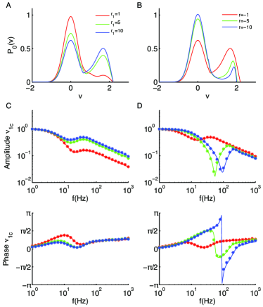
The dependence of $P_{0}(v)$ on $r_{1}$ and $r$ is shown in Fig. 2A-B. With the increase of $r_{1}$, the transition from the up state to the down state becomes more difficult, therefore the MP resides on the up state for a longer time (Fig. 1B), indicating a larger ratio between the maximal probability density at the up state and down state (Fig. 2A). Note that changing the slope $r_{1}$ can determine whether the up state exists or not by adjusting $v_{1}$, but does not influence the position of $v_{up}$ if it exists. With the increase of $|r|$ (the absolute value of $r$), $v_{up}$ is shifted slightly towards the higher deterministic fixed point and the ratio $P_{0}^{up}/P_{0}^{down}$ decreases (Fig. 2B).

Linear response- Now consider a weak sinusoidal signal encoded in the mean input, $\mu(t)=\mu+\varepsilon\cos(\omega t)$, where $\varepsilon$ is small. At the linear order in $\varepsilon$, the instantaneous firing rate is given by $\nu(t)=\nu_{0}+\varepsilon|\nu_{1c}(\omega)|\cos(\omega t-\phi_{c}(\omega))$, where $|\nu_{1c}(\omega)|$ is the transmission function and $\phi_{c}(\omega)$ is the phase lag. We find that a complex response function $\nu_{1c}(\omega)$ can be obtained analytically by solving the FPE at the linear order using the Green’s function method. The transmission function is the absolute value of $\nu_{1c}(\omega)$, while the phase lag $\phi_{c}(\omega)$ is given by the phase angle, $\phi_{c}(\omega)=\arg(\nu_{1c}(\omega))$. The expression of $\nu_{1c}(\omega)$ reads

$$\nu_{1c}(\omega)=\frac{1}{B}\bigg{[}\frac{i\omega(1+1/r_{1})}{(1-i\omega)(1+i\omega/r_{1})}(\psi_{1}P_{01}-\sqrt{D}\Phi_{1}P_{01}^{{}^{\prime}})$$

$$+\frac{i\omega(1/r_{1}-1/r)}{(1+i\omega_{/}r)(1+i\omega/r_{1})}(\psi_{1}Y_{5}^{{}^{\prime}}-\psi_{1}^{{}^{\prime}}Y_{5})P_{02}(v_{1})\;e^{\Delta_{1}}$$

$$+\frac{\sqrt{Dr_{1}}(r-r_{1})}{(r_{1}+i\omega)(r+i\omega)}(\psi_{1}Y_{51}^{{}^{\prime}}-\psi_{1}^{{}^{\prime}}Y_{51})P_{02}^{{}^{\prime}}(v_{1})\;e^{\Delta_{1}}$$

$$+\frac{\nu_{0}/\sqrt{Dr_{1}}}{1+i\omega/r_{1}}(\psi_{1}Y_{51r}^{{}^{\prime}}-\psi_{1}^{{}^{\prime}}Y_{51r})e^{\Delta_{0}}-\frac{\nu_{0}/\sqrt{D|r|}}{1+i\omega/r}\times$$

$$\quad((\psi_{1}Y_{5}^{{}^{\prime}}-\psi_{1}^{{}^{\prime}}Y_{5})Y_{2}^{{}^{\prime}}-(\psi_{1}Y_{6}^{{}^{\prime}}-\psi_{1}^{{}^{\prime}}Y_{6})Y_{2})e^{\Delta_{2}}\bigg{]}\;,$$ (6)

where $\psi_{1}(v)$, $\Phi_{1}(v)$, etc. are parabolic cylinder functions abramowitz , and $Y_{1}(v)$, $Y_{5}(v)$, $B$, etc. are combinations of them to simplify the expressions, as defined in sup . Note the functions adopt their values at $v=v_{0}$, unless denoted otherwise. Taking $\omega\to\infty$ in Eq. (Impact of membrane bistability on dynamical response of neuronal populations), we find that the high frequency limit is the same as the LIF model and the $r-\tau$ model, i.e., $\nu_{1c}\to\frac{\nu_{0}}{\sqrt{D}}\frac{1}{\sqrt{\omega}}\;e^{i\frac{\pi}{4}}$. This high frequency limit is characteristic of the linear dynamics and absorbing boundary wei .

Figure 2: Dependence of probability density and linear response on $r_{1}$ and $r$. A and B, probability density for different $r_{1}$ and $r$. C and D, dependence of the transmission function (upper panels) and phase lag (lower panels) of the linear response on $r_{1}$ and $r$. The linear response is normalized with the value at $f=1\;\textrm{Hz}$. Signal frequency $f$ is related to the angular frequency $\omega$ by $\omega=2\pi f$. Solid lines are from theoretical results and asterisks are from simulations. Parameters used: $r=-1$ in A and C, $r_{1}=10$ in B and D. Other parameters are the same as in Fig. 1.

Frequency-selective enhancement of linear response by the up state- The dependence of the linear response on $r_{1}$ and $r$ are shown in Fig. 2C-D. We see that a local maximum, denoted as $\nu_{1c}^{max}$, appears at frequency $f^{max}$ (Fig. 2C-D, upper panels) accompanying the development of the up state (Fig. 2A-B). The local maximal value of transmission function at the resonance frequency increases with $r_{1}$ and decreases with $|r|$, following the same trend as the ratio between the probability density at $v_{up}$ and $v_{down}$ (Fig. 2A-B). The phase lag of the firing rate response relative to the input signal is reduced when there is a more pronounced up state (Fig. 2C-D, lower panels). Therefore the up state can enhance the dynamical response by developing local maximum at some specific resonance frequency, and reduce the phase lag of the response.

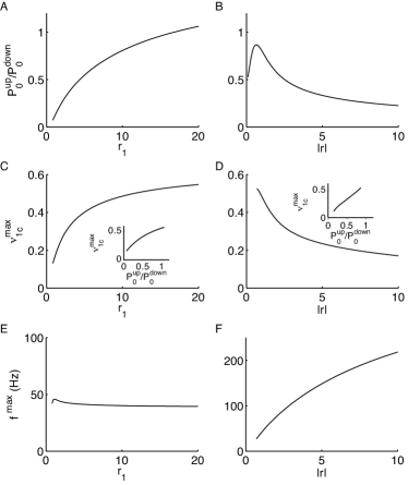
We characterize the relationship between the up state occupancy and resonance in the linear response quantitatively in Fig. 3. While the ratio between probability densities at $v_{up}$ and $v_{down}$ increases with $r_{1}$ (Fig. 3A), the maximal value of the transmission function at the resonance frequency also increases with $r_{1}$ (Fig. 3C). This leads to an increase of $\nu_{1c}^{max}$ with $P_{0}^{up}/P_{0}^{down}$ (Fig. 3C, inset). Similarly, $\nu_{1c}^{max}$ decreases with $|r|$ (Fig. 3D), following with the same trend as $P_{0}^{up}/P_{0}^{down}$ except for an initial small $|r|$ regime where there is no local maximum for $|\nu_{1c}(\omega)|$ (Fig. 3B). This also leads to an increase of $\nu_{1c}^{max}$ with $P_{0}^{up}/P_{0}^{down}$ (Fig. 3D, inset). The signal frequency at which the transmission function is maximally enhanced, $f^{max}$, keeps constant when $r_{1}$ increases, i.e., being independent of the time scale characterizing the unstable fixed point. On the contrary, $f^{max}$ goes to higher frequencies when $|r|$ increases, therefore is determined by the membrane time constant at the up state, $\tau/|r|$.

Figure 3: Dependence of up state occupancy and resonance in the linear response on $r_{1}$ and $r$. A and B, the up state Occupancy $P_{0}^{up}/P_{0}^{down}$ as a function of $r_{1}$ (A) and $|r|$ (B). C and D, the local maximal value $\nu_{1c}^{max}$ of the normalized transmission function as a function of $r_{1}$ (C) and $|r|$ (D). E and F, the resonance frequency $f^{max}$ as a function of $r_{1}$ (E) and $|r|$ (F). Insets: $\nu_{1c}^{max}$ as a function of $P_{0}^{up}/P_{0}^{down}$ due to the change of $r_{1}$ (C) and and $|r|$ (D). Parameters used: $r=-1$ in A and $r_{1}=10$ in B. Other parameters are the same as in Fig. 1.

We tested the predication by using a neuron model with biophysically realistic membrane currents, which includes a noninactivating potassium current controlling the up state and an inward rectifying potassium current stabilizing the down state compte . We find that the normalized frequency response is strongly enhanced with the development of the up state sup .

Discussion- Dynamical response to noisy oscillatory inputs is a fundamental characterization of neurons’ capability in signal encoding and transmission. Our model predicts a frequency-selective enhancement of signal transmission with the development of the up state. This prediction can be experimentally tested for neurons exhibiting up and down states by performing experiments similar to that in kondgen . Selective enhancement of specific high frequency component of signals might be functionally beneficial for neural communication, since signals with frequencies within the gamma band (30-100 Hz) or “high gamma” ($>100$ Hz) have been suggested to synchronize inter-regional brain activity gamma . Bistable piecewise linear membrane dynamics was introduced previously to approximate the nullcline of MP in the FitzHugh-Nagumo model mckean . In the limit of $\tau\to 0$, the linear response of that system was obtained lindner1 . Here we obtain the linear response analytically for a one-dimensional bistable system with general $\tau$. Bistability in individual neurons provides an alternative explanation for persistent activity in some brain areas marder , and is related to perfect temporal information accumulation okamoto and self-organized criticality millman . Our work sheds insights into the possible role of the up state on signal encoding and transmission through population response. Further work on building a network of interconnected such bistable units is needed to examine the relationship between the up state at the individual neuron level and at the circuit level stern .

We thank J. Mejias, J. Murray and F. Song for carefully reading the manuscript.

References

- (1) R. Llinas and M. Sugimori, J. Physiol. (London) 305, 171 (1980); C. Wilson and Y. Kawaguchi, J. Neurosci. 16, 2397 (1996) R. Lee and C. Heckman, J. Neurophysiol. 80, 583 (1998); I. Lamp et al., Neuron 22, 361 (1999); J. Anderson et al., Nat. Neurosci. 3, 617 (2000); M. Sanchez-Vives and D. McCormick, Nat. Neurosci. 3, 1027 (2000); P. Heyward et al., J. Neurosci. 21, 5311 (2001); S. William et al., J. Physiol. (London) 539, 469 (2002); Y. Loewenstein et al., Nat. Neurosci. 8, 202 (2005).
- (2) N. Parga and L. F. Abbott, Front. Neurosci. 1, 57 (2007).
- (3) A. Compte et al., J. Neurophysiol. 89, 2707 (2003).
- (4) M. Shadlen and W. Newsome, J. Neurosci. 18, 3870 (1998).
- (5) B. Knight, J. Gen. Physiol. 59, 734 (1972); W. Gerstner, Neural Comput. 12, 43 (2000).
- (6) H. Köndgen et al., Cereb. Cortex 18, 2086 (2008); C. Boucsein et al., J. Neurosci. 29, 1006 (2009); M. Higgs and W. Spain, J. Neurosci. 29, 1285 (2009); T. Tchumatchenko et al., J. Neurosci. (2012); V. Ilin et al., J. Neurosci. 33, 15915 (2013).
- (7) N. Brunel et al., Phys. Rev. Lett. 86, 2186 (2001); B. Lindner and L. Schimansky-Geier, Phys. Rev. Lett. 86, 2934 (2001)
- (8) W. Wei and F. Wolf, Phys. Rev. Lett. 18, 297 (2011).
- (9) N. Fourcaud-Trocmè et al., J. Neurosci. 23, 11628 (2003); N. Fourcaud-Trocmè et al., J. Comput. Neurosci. 18, 311 (2005); C. Geisler et al., J. Neurophysiol. 94, 4344 (2005); B. Naundorf et al., J. Comput. Neurosci. 18, 297 (2005); M. Richardson, Phy. Rev. E 76, 021919 (2007).
- (10) I. Timofeev et al., Proc. Natl. Acad. Sci. 98, 1924 (2001).
- (11) C. van Vreeswijk and H. Sompolinsky, Science 274, 1724 (1996).
- (12) H. Risken, The Fokker Planck Equation: Methods of Solution and Applications (Springer-Verlag, Berlin, 1984).
- (13) M. Abramowitz and I. A. Stegun, Tables of Mathematical Functions (Dover Publications, New York, 1970).
- (14) Supplementary material for the paper.
- (15) X.-J. Wang, Physiol. Rev. 90, 1195 (2010); G. Buzsáki and X.-J. Wang, Annu. Rev. Neurosci. 35, 203 (2012); G. Buzsáki and E. Schomburg, Nature Neurosci., advance online publication (2015).
- (16) H. McKean, Advances in Mathematics, 4, 209 (1970).
- (17) B. Lindner and L. Schimansky-Geier, Phys. Rev. E 93, 13481 (2000).
- (18) E. Marder et al., Proc. Natl. Acad. Sci. 98, 1924 (1996); M. Camperi and X.-J. Wang, J. Comput. Neurosci. 5, 383 (1998).
- (19) H. Okamoto and T. Fukai, PLoS Comput. Biol. 5, e1000404 (2009).
- (20) D. Millman et al., Nature Physics 6, 801 (2010).
- (21) M. Stern, H. Sompolinsky, and L. F. Abbott, Phys. Rev. E 90, 062710 (2014).