The two-loop helicity amplitudes for $gg\to V_{1}V_{2}\to 4~{}\mathrm{leptons}$

Abstract

We compute the two-loop massless QCD corrections to the helicity amplitudes for the production of two electroweak gauge bosons in the gluon fusion channel, $gg\to V_{1}V_{2}$, keeping the virtuality of the vector bosons $V_{1}$ and $V_{2}$ arbitrary and taking their decays into leptons into account. The amplitudes are expressed in terms of master integrals, whose representation has been optimised for fast and reliable numerical evaluation. We provide analytical results and a public C++ code for their numerical evaluation on HepForge at http://vvamp.hepforge.org.

1 Introduction

Pair production processes for electroweak vector bosons provide a rich spectrum of observables, which are crucial to test in depth the $SU(2)_{L}\times U(1)_{Y}$ gauge sector of the Standard Model. In particular, the production of pairs of resonant vector bosons allows for precise studies of the electroweak triple gauge couplings, while considering off-shell vector boson pairs is required for precision Higgs phenomenology. Furthermore, diboson production processes are important backgrounds in direct new physics searches. The main production channel for pairs of vector bosons at hadron colliders is quark-antiquark annihilation and great progress has been achieved in the last years with the computation of the next-to-next-to-leading order (NNLO) QCD corrections to $q\bar{q}\to\gamma\gamma$ Catani:2011qz , $q\bar{q}\to Z\gamma$ Grazzini:2013bna , $q\bar{q}\to ZZ$ Cascioli:2014yka and $q\bar{q}\to W^{+}W^{-}$ Gehrmann:2014fva production at the LHC. Furthermore, the fermionic NNLO corrections to $q\bar{q}\to\gamma^{*}\gamma^{*}$ were derived in Anastasiou:2014nha .

The gluon fusion channel contributes to $\gamma\gamma$, $ZZ$, $Z\gamma$ and $W^{+}W^{-}$ production. As a quark-loop induced process, its leading order (LO) cross section is suppressed by two powers of $\alpha_{s}$ with respect to that of the quark channel. This implies that it formally contributes only at NNLO in the perturbative expansion of the hadronic process, but numerical enhancements may be expected due to the large gluon luminosities at typical energies for diboson production at the LHC. For the gluon-induced processes, the one-loop amplitudes and the corresponding one-loop squared interference terms have been computed long ago Costantini:1971cj ; vanderBij:1988fb ; Glover:1988rg ; Glover:1988fe ; Adamson:2002jb ; Adamson:2002rm ; Binoth:2006mf . Their impact on the total cross section was found to range approximately from $5\%$ to more than $10\%$ for different final states at the LHC, and to rise with increasing collider energy Catani:2011qz ; Grazzini:2013bna ; Cascioli:2014yka ; Gehrmann:2014fva . These values can substantially increase up to about $30\%$ when particular sets of cuts, relevant for example for Higgs boson searches, are applied Binoth:2005ua ; Cascioli:2013gfa . It is therefore clear that the inclusion of gluon channel contributions can be important in order to achieve a description of the full process which matches the experimental precision. Beyond the actual size of the known leading order corrections in the gluon channel, it is unclear how large the associated theory uncertainty actually is. By comparison with Higgs production in gluon fusion Dawson:1990zj ; Djouadi:1991tka ; Spira:1995rr , the conventional LO scale variation is not expected to allow for a reliable estimate of the size of neglected higher order corrections. The recent NNLO predictions for the total $ZZ$ and $W^{+}W^{-}$ production cross sections take into account the quark channel at NNLO and the gluon channel at LO, resulting in a scale uncertainty of about $3\%$ Cascioli:2014yka ; Gehrmann:2014fva . In order to thoroughly control the theory uncertainty to this level of precision, it is therefore very desirable to compute the next-to-leading order (NLO) contributions for the gluon induced subprocess. Currently this has been done only for $gg\to\gamma\gamma$ Bern:2001df ; Bern:2002jx , and the NLO corrections have been found to be not only sizeable but also important for stabilising the theoretical predictions Bern:2002jx . Finally, precise theoretical predictions for $gg\to ZZ$ can be useful for constraining the total Higgs boson decay width at the LHC Campbell:2011cu ; Kauer:2012hd ; Caola:2013yja ; Campbell:2013una .

Technically, the computation of the NLO corrections to $gg\to V_{1}V_{2}$ requires two ingredients, the two-loop virtual corrections to $gg\to V_{1}V_{2}$ and the one-loop real-virtual corrections to the corresponding radiative processes with one more parton in the final state. By now the computation of the one-loop amplitudes with an extra gluon does not constitute any conceptual difficulty and can be pursued with standard techniques for one-loop multi-legs processes Berger:2008sj ; Hirschi:2011pa ; Ellis:2011cr ; Bevilacqua:2011xh ; Cullen:2011ac ; Cascioli:2011va ; Cullen:2014yla . The two-loop amplitudes, on the other hand, are known only for $gg\to\gamma\gamma$ Bern:2001df and for $gg\to Z\gamma$ Gehrmann:2013vga , in both cases for on-shell final state photons. In order to obtain physical predictions, both contributions need to be combined using a subtraction scheme to isolate and cancel unphysical IR divergences. In this case, a NLO scheme Frixione:1995ms ; Catani:1996vz would be sufficient.

In this paper we calculate the missing two-loop massless QCD corrections to $gg\to V_{1}V_{2}$, with an off-shell vector boson pair $V_{1}V_{2}=\gamma^{*}\gamma^{*},ZZ,Z\gamma^{*},W^{+}W^{-}$. The calculation builds upon the master integrals for four-point functions with massless propagators and two massive external legs, which were computed recently in the case of equal masses in Gehrmann:2013cxs ; Gehrmann:2014bfa , and in the case of different masses in Henn:2014lfa ; Caola:2014lpa ; Papadopoulos:2014hla ; Gehrmann:2015ora . The former were used for the first NNLO fully-inclusive calculations of $ZZ$ Cascioli:2014yka and $W^{+}W^{-}$ Gehrmann:2014fva production at the LHC, while the latter allowed the computation of the two-loop corrections to $q\bar{q}^{\prime}\to V_{1}V_{2}$ Caola:2014iua ; Gehrmann:2015ora . A subset of these master integrals was also computed independently in Chavez:2012kn ; Anastasiou:2014nha . While the inclusion of massive top-loop mediated subprocesses would be of interest for some phenomenological applications Campbell:2011cu ; Melnikov:2015laa , the computation of the two-loop amplitudes requires knowledge of challenging new master integrals, which should be addressed in the future.

The paper is structured as follows. In Section 2 we describe the tensor decomposition of the partonic current for the process $gg\to V_{1}V_{2}$ and consider the possible electroweak coupling structures. We include the vector boson decays and describe the helicity amplitudes for the process $gg\to V_{1}V_{2}\to 4~{}\mathrm{leptons}$ in terms of scalar form factors in Section 3. The actual calculation of the loop contributions to these form factors is described in Section 4, which includes a dicussion of UV renormalisation, IR subtraction and various checks we performed on our results. In Section 5 we present numerical results obtained with our C++ implementation. Finally, we conclude in Section 6. In Appendix A we give explicit formulae for obtaining the physical form factors appearing in the helicity amplitudes from the original tensor coefficients computed in this paper. We provide computer readable files for our analytical results and our C++ code for the numerical evaluation of the amplitudes on our VVamp project page on HepForge at http://vvamp.hepforge.org.

2 Partonic current for $gg\to V_{1}V_{2}$

We consider the production of two massive off-shell vector bosons, $V_{1}V_{2}$, in the gluon fusion channel,

$$g(p_{1})+g(p_{2})\longrightarrow V_{1}(p_{3})+V_{2}(p_{4}),$$ (1)

where $V_{1}V_{2}$ = $\gamma^{*}\gamma^{*}$, $ZZ$, $Z\gamma^{*}$, $W^{+}W^{-}$. The final states $W^{\pm}\gamma^{*}$ and $W^{\pm}Z$ instead are forbidden by charge conservation. Since the two vector bosons are off-shell we have in the general case

$$p_{1}^{2}=p_{2}^{2}=0\,,\quad p_{3}^{2}>0,\quad p_{4}^{2}>0,\quad p_{3}^{2}\neq p_{4}^{2},$$ (2)

with the usual Mandelstam invariants defined as

$$s=(p_{1}+p_{2})^{2}\,,\qquad t=(p_{1}-p_{3})^{2}\,,\qquad u=(p_{2}-p_{3})^{2}\,,$$ (3)

and the relation

$$s+t+u=p_{3}^{2}+p_{4}^{2}\,.$$ (4)

The physical region for the scattering kinematics has the boundary $t\,u=p_{3}^{2}\,p_{4}^{2}$ and fulfils

$$s\geq\Big{(}\sqrt{p_{3}^{2}}+\sqrt{p_{4}^{2}}\Big{)}^{2},\qquad\frac{1}{2}\big{(}p_{3}^{2}+p_{4}^{2}-s-\kappa\big{)}\leq t\leq\frac{1}{2}\big{(}p_{3}^{2}+p_{4}^{2}-s+\kappa\big{)}$$ (5)

where $\kappa$ is the Källén function

$$\kappa\left(s,p_{3}^{2},p_{4}^{2}\right)\equiv\sqrt{s^{2}+p_{3}^{4}+p_{4}^{4}-2(s\,p_{3}^{2}+p_{3}^{2}\,p_{4}^{2}+p_{4}^{2}\,s)}\,.$$ (6)

We denote the scattering amplitude for the process (1) by

$$S(p_{1},p_{2},p_{3})=S_{\mu\nu\rho\sigma}(p_{1},p_{2},p_{3})\,\epsilon_{1}^{\rho}(p_{1})\,\epsilon_{2}^{\sigma}(p_{2})\,\epsilon_{3}^{\ast\,\mu}(p_{3})\,\epsilon_{4}^{\ast\,\nu}(p_{4})$$

where $\epsilon_{1}$, $\epsilon_{2}$ are the polarisation vectors of the incoming gluons, $\epsilon_{3}$, $\epsilon_{4}$ are the polarisation vectors of the outgoing massive vector bosons, $p_{4}=p_{1}+p_{2}-p_{3}$ and an overall factor $e^{2}$ is kept implicit with $e$ being the positron charge. Since we will consider leptonic decays of the massive vector bosons we will be able to construct the full amplitude including the decays from the partonic current

$$S_{\mu\nu}(p_{1},p_{2},p_{3})=S_{\mu\nu\rho\sigma}(p_{1},p_{2},p_{3})\,\epsilon_{1}^{\rho}(p_{1})\,\epsilon_{2}^{\sigma}(p_{2})$$

for the $2\to 2$ process. In particular, it is only the latter which receives (pure) QCD corrections at any order in perturbation theory.

In order to compute the partonic current it is useful to consider its tensor decomposition. Based on Lorentz invariance only, there are 138 independent tensor structures which can contribute

$$S^{\mu\nu\rho\sigma}(p_{1},p_{2},p_{3}) =a_{1}g^{\mu\nu}g^{\rho\sigma}+a_{2}g^{\mu\rho}g^{\nu\sigma}+a_{3}g^{\mu\sigma}g^{\nu\rho}$$

$$+\sum\limits_{j_{1},j_{2}=1}^{3}\Bigl{(}b^{(1)}_{j_{1}j_{2}}\,g^{\mu\nu}\,p_{j_{1}}^{\rho}\,p_{j_{2}}^{\sigma}+b^{(2)}_{j_{1}j_{2}}\,g^{\mu\rho}\,p_{j_{1}}^{\nu}\,p_{j_{2}}^{\sigma}+b^{(3)}_{j_{1}j_{2}}\,g^{\mu\sigma}\,p_{j_{1}}^{\nu}\,p_{j_{2}}^{\rho}$$

$$\phantom{\sum\limits_{j_{1},j_{2}=1}^{3}}+b^{(4)}_{j_{1}j_{2}}\,g^{\nu\rho}\,p_{j_{1}}^{\mu}\,p_{j_{2}}^{\sigma}+b^{(5)}_{j_{1}j_{2}}\,g^{\nu\sigma}\,p_{j_{1}}^{\mu}\,p_{j_{2}}^{\rho}+b^{(6)}_{j_{1}j_{2}}\,g^{\rho\sigma}\,p_{j_{1}}^{\mu}\,p_{j_{2}}^{\nu}\Bigr{)}$$

$$+\sum\limits_{j_{1},j_{2},j_{3},j_{4}=1}^{3}c_{j_{1}j_{2}j_{3}j_{4}}p_{j_{1}}^{\mu}\,p_{j_{2}}^{\nu}p_{j_{3}}^{\rho}\,p_{j_{4}}^{\sigma},$$ (7)

where the coefficients $a_{j}$, $b_{ij}^{k}$ and $c_{ijkl}$ are scalar functions of the kinematic invariants $s$, $t$, $p_{3}^{2}$, $p_{4}^{2}$ and of the space-time dimension $d$. Not all structures are relevant for our calculation. Many of them simply drop due to the transversality of the gluons’ polarisation vectors

$$\epsilon_{1}\cdot p_{1}=\epsilon_{2}\cdot p_{2}=0\,.$$ (8)

Moreover the tensor structure can be further simplified by fixing explicitly the gauge for the incoming gluons. A particularly simple choice is given by the symmetrical condition

$$\epsilon_{1}\cdot p_{2} =\epsilon_{2}\cdot p_{1}=0\,,$$ (9)

which corresponds to the following rules for the polarisation sums

$$\sum_{\lambda_{1}}\epsilon_{1\,\lambda_{1}}^{\mu*}(p_{1})\epsilon_{1\,\lambda_{1}}^{\nu}(p_{1}) =-g^{\mu\nu}+\frac{p_{1}^{\mu}p_{2}^{\nu}+p_{1}^{\nu}p_{2}^{\mu}}{p_{1}\cdot p_{2}}\,,$$

$$\sum_{\lambda_{2}}\epsilon_{2\,\lambda_{2}}^{\mu*}(p_{2})\epsilon_{2\,\lambda_{2}}^{\nu}(p_{2}) =-g^{\mu\nu}+\frac{p_{1}^{\mu}p_{2}^{\nu}+p_{1}^{\nu}p_{2}^{\mu}}{p_{1}\cdot p_{2}}\,.$$ (10)

Further conditions can be applied on the polarisation vectors of the massive vector bosons $V_{1}$, $V_{2}$. We employ for their polarisation vectors

$$\epsilon_{3}\cdot p_{3}=\epsilon_{4}\cdot p_{4}=0\,,$$ (11)

and for the polarisation sums

$$\sum_{\lambda_{3}}\epsilon_{3\,\lambda_{3}}^{\mu*}(p_{3})\epsilon_{3\,\lambda_{3}}^{\nu}(p_{3}) =-g^{\mu\nu}+\frac{p_{3}^{\mu}p_{3}^{\nu}}{p_{3}^{2}}\,,$$

$$\sum_{\lambda_{4}}\epsilon_{4\,\lambda_{4}}^{\mu*}(p_{4})\epsilon_{4\,\lambda_{4}}^{\nu}(p_{4}) =-g^{\mu\nu}+\frac{p_{4}^{\mu}p_{4}^{\nu}}{p_{4}^{2}}\,.$$ (12)

Imposing the constraints (8), (9) and (11) one is left with only $20$ independent tensor structures and we can write the partonic current according to

$$S^{\mu\nu}(p_{1},p_{2},p_{3}) =\sum_{j=1}^{20}\,A_{j}(s,t,p_{3}^{2},p_{4}^{2})\,T_{j}^{\mu\nu}\,,$$ (13)

where the $A_{j}$ are scalar functions of $s$, $t$, $p_{3}^{2}$, $p_{4}^{2}$ and $d$. The tensors $T^{\mu\nu}_{j}$ are defined as

$$\begin{aligned} T_{1}^{\mu\nu}&=\epsilon_{1}\cdot\epsilon_{2}\,g^{\mu\nu}\,,&T_{2}^{\mu\nu}&=\epsilon_{1}^{\mu}\,\epsilon_{2}^{\nu}\,,&T_{3}^{\mu\nu}&=\epsilon_{1}^{\nu}\,\epsilon_{2}^{\mu}\,,&T_{4}^{\mu\nu}&=\epsilon_{1}\cdot\epsilon_{2}\,p_{1}^{\mu}\,p_{1}^{\nu}\,,\\ T_{5}^{\mu\nu}&=\epsilon_{1}\cdot\epsilon_{2}\,p_{1}^{\mu}\,p_{2}^{\nu}\,,&T_{6}^{\mu\nu}&=\epsilon_{1}\cdot\epsilon_{2}\,p_{2}^{\mu}\,p_{1}^{\nu}\,,&T_{7}^{\mu\nu}&=\epsilon_{1}\cdot\epsilon_{2}\,p_{2}^{\mu}\,p_{2}^{\nu}\,,&T_{8}^{\mu\nu}&=\epsilon_{2}\cdot p_{3}\,\epsilon_{1}^{\mu}\,p_{1}^{\nu}\,,\\ T_{9}^{\mu\nu}&=\epsilon_{2}\cdot p_{3}\,\epsilon_{1}^{\mu}\,p_{2}^{\nu}\,,&T_{10}^{\mu\nu}&=\epsilon_{2}\cdot p_{3}\,\epsilon_{1}^{\nu}\,p_{1}^{\mu}\,,&T_{11}^{\mu\nu}&=\epsilon_{2}\cdot p_{3}\,\epsilon_{1}^{\nu}\,p_{2}^{\mu}\,,&T_{12}^{\mu\nu}&=\epsilon_{1}\cdot p_{3}\,\epsilon_{2}^{\mu}\,p_{1}^{\nu}\,,\\ T_{13}^{\mu\nu}&=\epsilon_{1}\cdot p_{3}\,\epsilon_{2}^{\mu}\,p_{2}^{\nu}\,,&T_{14}^{\mu\nu}&=\epsilon_{1}\cdot p_{3}\,\epsilon_{2}^{\nu}\,p_{1}^{\mu}\,,&T_{15}^{\mu\nu}&=\epsilon_{1}\cdot p_{3}\,\epsilon_{2}^{\nu}\,p_{2}^{\mu}\,,&T_{16}^{\mu\nu}&=\epsilon_{1}\cdot p_{3}\,\epsilon_{2}\cdot p_{3}\,g^{\mu\nu}\,,\end{aligned}$$

$$\begin{aligned} T_{17}^{\mu\nu}&=\epsilon_{1}\cdot p_{3}\,\epsilon_{2}\cdot p_{3}\,p_{1}^{\mu}\,p_{1}^{\nu}\,,&T_{18}^{\mu\nu}&=\epsilon_{1}\cdot p_{3}\,\epsilon_{2}\cdot p_{3}\,p_{1}^{\mu}\,p_{2}^{\nu}\,,\end{aligned}$$

$$\begin{aligned} T_{19}^{\mu\nu}&=\epsilon_{1}\cdot p_{3}\,\epsilon_{2}\cdot p_{3}\,p_{2}^{\mu}\,p_{1}^{\nu}\,,&T_{20}^{\mu\nu}&=\epsilon_{1}\cdot p_{3}\,\epsilon_{2}\cdot p_{3}\,p_{2}^{\mu}\,p_{2}^{\nu}\,.\end{aligned}$$ (14)

We stress that the tensor decomposition (13) is based only on Lorentz symmetry, gauge invariance and the properties of the boson decays and holds therefore at every order in perturbative QCD. Moreover, no assumption has been made on the dimensionality of space-time and the result is valid for any values of the parameter $d$.

The scalar form factors $A_{j}$ can be extracted from the amplitude (13) by applying suitable projecting operators. The projectors themselves can be decomposed in the same $20$ tensors as

$$P_{j}^{\mu\nu}=\sum_{i=1}^{20}B_{ji}\left(T_{i}^{\mu\nu}\right)^{\dagger}\qquad\text{for~{}}j=1,\ldots,20,$$ (15)

where also $B_{ji}$ are functions of the external invariants and $d$. Their explicit form can be determined imposing

$$\sum_{pol}P_{j}^{\mu^{\prime}\nu^{\prime}}\left[\epsilon_{3\mu^{\prime}}\epsilon_{4\nu^{\prime}}\epsilon_{3\mu}^{*}\epsilon_{4\nu}^{*}\right]S^{\mu\nu} =A_{j}\quad\text{for~{}}j=1,...,20,$$ (16)

where the polarisation sums are evaluated in $d$ dimensions according to (10) and (12). The explicit results for the coefficients $B_{ji}$ are rather lengthy and we prefer not to write them here explicitly. Computer readable files for the latter are given on our project page at HepForge.

The partonic current is the only one which receives contributions from QCD radiative corrections and, for two gluons of helicities $\lambda_{1}$ and $\lambda_{2}$, can be written as

$$S_{\mu\nu}(p_{1}^{\lambda_{1}},p_{2}^{\lambda_{2}},p_{3})=\delta^{a_{1}a_{2}}\,\sum_{j}\mathcal{C}_{V_{1}V_{2}}^{[j]}\,S^{[j]}_{\mu\nu\rho\sigma}(p_{1},p_{2},p_{3})\epsilon_{1\lambda_{1}}^{\rho}(p_{1})\epsilon_{2\lambda_{2}}^{\sigma}(p_{2})\,,$$ (17)

where $\delta^{a_{1}a_{2}}$ is the overall colour structure and the index $j$ runs over different possible classes of diagrams discussed below, see also Fig. 1, which are characterised by different electroweak couplings $\mathcal{C}^{[j]}_{V_{1}V_{2}}$.

Before proceeding, it is convenient to introduce some notations needed in the following. As long as we work in QCD, we only need to consider the coupling of electroweak vector bosons $V$ to fermions. We follow Denner:1991kt and parametrise the couplings as

$$\mathcal{V}_{\mu}^{Vf_{1}f_{2}}=i\,e\,\Gamma_{\mu}^{Vf_{1}f_{2}}\,,\qquad\mbox{where}\quad e=\sqrt{4\,\pi\,\alpha}\quad\mbox{is the positron charge}\,,$$ (18)

such that all fermion charges are expressed in units of $e$ and

$$\Gamma_{\mu}^{Vf_{1}f_{2}}=L_{f_{1}f_{2}}^{V}\,\gamma_{\mu}\left(\frac{1-\gamma_{5}}{2}\right)+R_{f_{1}f_{2}}^{V}\,\gamma_{\mu}\left(\frac{1+\gamma_{5}}{2}\right)\,,$$ (19)

with

$$L_{f_{1}f_{2}}^{\gamma} =-e_{f_{1}}\,\delta_{f_{1}f_{2}} R_{f_{1}f_{2}}^{\gamma} =-e_{f_{1}}\,\delta_{f_{1}f_{2}}\,,$$ (20)

$$L_{f_{1}f_{2}}^{Z} =\frac{I_{3}^{f_{1}}-\sin^{2}{\theta_{w}}e_{f_{1}}}{\sin{\theta_{w}}\cos{\theta_{w}}}\,\delta_{f_{1}f_{2}}\,, \qquad R_{f_{1}f_{2}}^{Z} =-\frac{\sin{\theta_{w}}e_{f_{1}}}{\cos{\theta_{w}}}\,\delta_{f_{1}f_{2}}\,,$$ (21)

$$L_{f_{1}f_{2}}^{W} =\frac{1}{\sqrt{2}\,\sin{\theta_{w}}}\,\epsilon_{f_{1}f_{2}}\,, R_{f_{1}f_{2}}^{W} =0\,,$$ (22)

where $\epsilon_{f_{1}f_{2}}$ is unity for $f_{1}\neq f_{2}$, but belonging to the same isospin doublet, and zero otherwise.

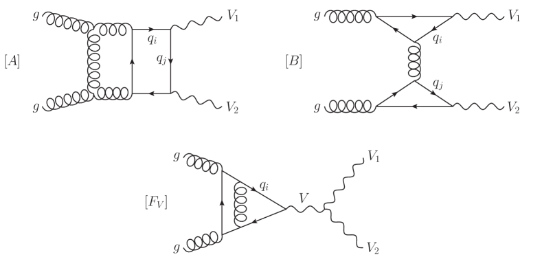
Figure 1: Example Feynman diagrams for the process $gg\to V_{1}V_{2}$ at the two-loop level, where the vector bosons couple to the same fermion loop, $[A]$, to different fermion loops, $[B]$, or to an intermediate vector boson, $[F_{V}]$. The sum of all type $[B]$ contribution and the sum of all type $[F_{V}]$ contributions vanish, respectively.

Let us consider the different electroweak coupling structures in detail. It is clear that, since we do not take any electroweak radiative corrections into account, at least one of the two vector bosons must be coupled to an internal fermion loop. In order to compute the one- and two-loop massless QCD corrections we need to consider the following three possibilities, see Fig. 1.

Class $\mathbf{A}$:

Both vector bosons $V_{1}V_{2}$ are attached to the same fermion loop. In this case the diagrams are proportional to the charge weighted sum of the quark flavours, which we denote as $\mathcal{C}_{V_{1}V_{2}}^{[A]}=N_{V_{1}V_{2}}$. These diagrams could in principle yield two different contributions. One, proportional to the sum of the vector-vector and the axial-axial couplings, in which all dependence on $\gamma_{5}$ cancels out. The second, instead, contains the vector-axial coupling and is linear in $\gamma_{5}$. Due to charge parity conservation this last contribution is expected to always vanish identically for massless quarks running in the loops, for any choice of $V_{1}$ and $V_{2}$ Glover:1988rg ; Glover:1988fe ; Melnikov:2015laa . One then easily finds that

$$N_{\gamma\gamma} =\frac{1}{2}\sum_{i}\left[\left(L_{q_{i}q_{i}}^{\gamma}\right)^{2}+\left(R_{q_{i}q_{i}}^{\gamma}\right)^{2}\right], N_{Z\gamma} =\frac{1}{2}\sum_{i}\left(L_{q_{i}q_{i}}^{Z}L_{q_{i}q_{i}}^{\gamma}+R_{q_{i}q_{i}}^{Z}R_{q_{i}q_{i}}^{\gamma}\right),$$

$$N_{ZZ} =\frac{1}{2}\sum_{i}\left[\left(L_{q_{i}q_{i}}^{Z}\right)^{2}+\left(R_{q_{i}q_{i}}^{Z}\right)^{2}\right], N_{WW} =\frac{1}{2}\sum_{i,\,j}\left(L_{q_{i}q_{j}}^{W}L_{q_{j}q_{i}}^{W}\right),$$ (23)

where the indices $i,j$ run over the flavours of the quarks in the loop and $L_{q_{i}q_{i}}^{\gamma}=R_{q_{i}q_{i}}^{\gamma}$ such that $N_{\gamma\gamma}=\sum_{i}e_{q_{i}}^{2}$.

Class $\mathbf{B}$:

The two vector bosons are attached to two different fermion loops. This configuration is of course possible only starting from two loops on. Each fermion loop contains both a vector and an axial piece. For the case of two-loop massless QCD corrections relevant here, both contributions can be shown to vanish. The axial contribution cancels out for degenerate isospin doublets, while the vector piece must sum up to zero due to Furry’s theorem.

Classes $\mathbf{F_{V}}$:

Only for the case of $V_{1}V_{2}=W^{+}W^{-}$, one should also take into account the $s$-channel production diagrams, where the incoming gluons produce an intermediate electroweak gauge boson $V=\gamma^{*}/Z^{*}$, which then decays into the outgoing $W$-pair, see Fig. 1. Charge-parity invariance ensures that the vector part of these diagrams must sum up to zero. Again, the axial part cancels out for degenerate isospin doublets, and therefore also in the case of massless quarks running in the loops.

For the case of the one- and two-loop contributions considered here, we can therefore simplify (17) to

$$S_{\mu\nu}(p_{1}^{\lambda_{1}},p_{2}^{\lambda_{2}},p_{3}) =\delta^{a_{1}a_{2}}\,N_{V_{1}V_{2}}\,S^{[A]}_{\mu\nu\rho\sigma}(p_{1},p_{2},p_{3})\epsilon_{1\lambda_{1}}^{\rho}(p_{1})\epsilon_{2\lambda_{2}}^{\sigma}(p_{2})\,,$$ (24)

with $N_{V_{1}V_{2}}$ given in (Class $\mathbf{A}$:) and consider the coefficients $A_{j}^{[A]}$ defined by

$$A_{j}(s,t,p_{3}^{2},p_{4}^{2}) =\delta_{a_{1}a_{2}}N_{V_{1}V_{2}}A_{j}^{[A]}(s,t,p_{3}^{2},p_{4}^{2}).$$ (25)

It is instructive to study the transformations of the partonic current (24) under permutations of the external legs. We define the following two permutations

$$\pi_{12}:=p_{1}\leftrightarrow p_{2}\Rightarrow\{\,t\leftrightarrow u\,\},$$

$$\pi_{34}:=p_{3}\leftrightarrow p_{4}\Rightarrow\{\,t\leftrightarrow u\,,\;\;p_{3}^{2}\leftrightarrow p_{4}^{2}\,\}\,.$$ (26)

Because of Bose symmetry these two permutations must leave the partonic amplitude unchanged. This enforces a well defined behaviour of the coefficients $A_{j}(s,t,p_{3}^{2},p_{4}^{2})$ under the action of $\pi_{12}$ and $\pi_{34}$. From direct inspection of (13) one finds that the following relations must be fulfilled:

$$\pi_{12}:\quad A^{[A]}_{1}(s,u,p_{3}^{2},p_{4}^{2}) =A^{[A]}_{1}(s,t,p_{3}^{2},p_{4}^{2})\,,\qquad A^{[A]}_{2}(s,u,p_{3}^{2},p_{4}^{2}) =A^{[A]}_{3}(s,t,p_{3}^{2},p_{4}^{2})\,,$$

$$A^{[A]}_{4}(s,u,p_{3}^{2},p_{4}^{2}) =A^{[A]}_{7}(s,t,p_{3}^{2},p_{4}^{2})\,, A^{[A]}_{5}(s,u,p_{3}^{2},p_{4}^{2}) =A^{[A]}_{6}(s,t,p_{3}^{2},p_{4}^{2})\,,$$

$$A^{[A]}_{8}(s,u,p_{3}^{2},p_{4}^{2}) =A^{[A]}_{13}(s,t,p_{3}^{2},p_{4}^{2})\,, A^{[A]}_{9}(s,u,p_{3}^{2},p_{4}^{2}) =A^{[A]}_{12}(s,t,p_{3}^{2},p_{4}^{2})\,,$$

$$A^{[A]}_{10}(s,u,p_{3}^{2},p_{4}^{2}) =A^{[A]}_{15}(s,t,p_{3}^{2},p_{4}^{2})\,, A^{[A]}_{11}(s,u,p_{3}^{2},p_{4}^{2}) =A^{[A]}_{14}(s,t,p_{3}^{2},p_{4}^{2})\,,$$

$$A^{[A]}_{16}(s,u,p_{3}^{2},p_{4}^{2}) =A^{[A]}_{16}(s,t,p_{3}^{2},p_{4}^{2})\,, A^{[A]}_{17}(s,u,p_{3}^{2},p_{4}^{2}) =A^{[A]}_{20}(s,t,p_{3}^{2},p_{4}^{2})\,,$$

$$A^{[A]}_{18}(s,u,p_{3}^{2},p_{4}^{2}) =A^{[A]}_{19}(s,t,p_{3}^{2},p_{4}^{2})\,,$$ (27)

$$\pi_{34}:\quad A^{[A]}_{1}(s,u,p_{4}^{2},p_{3}^{2}) =A^{[A]}_{1}(s,t,p_{3}^{2},p_{4}^{2})\,, A^{[A]}_{2}(s,u,p_{4}^{2},p_{3}^{2}) =A^{[A]}_{3}(s,t,p_{3}^{2},p_{4}^{2})\,,$$

$$A^{[A]}_{4}(s,u,p_{4}^{2},p_{3}^{2}) =A^{[A]}_{4}(s,t,p_{3}^{2},p_{4}^{2})\,, A^{[A]}_{5}(s,u,p_{4}^{2},p_{3}^{2}) =A^{[A]}_{6}(s,t,p_{3}^{2},p_{4}^{2})\,,$$

$$A^{[A]}_{7}(s,u,p_{4}^{2},p_{3}^{2}) =A^{[A]}_{7}(s,t,p_{3}^{2},p_{4}^{2})\,, A^{[A]}_{8}(s,u,p_{4}^{2},p_{3}^{2}) =-A^{[A]}_{10}(s,t,p_{3}^{2},p_{4}^{2})\,,$$

$$A^{[A]}_{9}(s,u,p_{4}^{2},p_{3}^{2}) =-A^{[A]}_{11}(s,t,p_{3}^{2},p_{4}^{2})\,, A^{[A]}_{12}(s,u,p_{4}^{2},p_{3}^{2}) =-A^{[A]}_{14}(s,t,p_{3}^{2},p_{4}^{2})\,,$$

$$A^{[A]}_{13}(s,u,p_{4}^{2},p_{3}^{2}) =-A^{[A]}_{15}(s,t,p_{3}^{2},p_{4}^{2})\,, A^{[A]}_{16}(s,u,p_{4}^{2},p_{3}^{2}) =A^{[A]}_{16}(s,t,p_{3}^{2},p_{4}^{2})\,,$$

$$A^{[A]}_{17}(s,u,p_{4}^{2},p_{3}^{2}) =A^{[A]}_{17}(s,t,p_{3}^{2},p_{4}^{2})\,, A^{[A]}_{18}(s,u,p_{4}^{2},p_{3}^{2}) =A^{[A]}_{19}(s,t,p_{3}^{2},p_{4}^{2})\,,$$

$$A^{[A]}_{20}(s,u,p_{4}^{2},p_{3}^{2}) =A^{[A]}_{20}(s,t,p_{3}^{2},p_{4}^{2})\,,$$ (28)

It is interesting to notice that, upon exploiting all of these crossing relations, only $9$ out of the $20$ coefficients $A_{j}^{[A]}$ turn out to be effectively independent, while the other $11$ coefficients can be obtained by crossing of the external legs.

3 Helicity amplitudes for $gg\to V_{1}V_{2}\to 4~{}\mathrm{leptons}$

We consider physical processes, where the two off-shell vector bosons decay into lepton pairs

$$g(p_{1})+g(p_{2})\rightarrow V_{1}(p_{3})+V_{2}(p_{4})\rightarrow l_{5}(p_{5})+\bar{l}_{6}(p_{6})+l_{7}(p_{7})+\bar{l}_{8}(p_{8})$$ (29)

such that $p_{3}=p_{5}+p_{6}\,$, $\,p_{4}=p_{7}+p_{8}$ and $p_{5}^{2}=p_{6}^{2}=p_{7}^{2}=p_{8}^{2}=0$. As long as we consider QCD radiative corrections the amplitudes $\mathcal{M}_{\lambda_{1}\lambda_{2}\lambda_{3}\lambda_{4}}^{V_{1}V_{2}}$ can be written, at any order in perturbation theory, as the product of the partonic current for $gg\to V_{1}V_{2}$ with the two leptonic currents for the decay products, $V_{1}\to l_{5}\bar{l}_{6}$ and $V_{2}\to l_{7}\bar{l}_{8}$, mediated by the propagators of the two off-shell vector bosons $V_{1}$ and $V_{2}$. We write the propagator for an off-shell vector boson in the $R_{\xi}$ gauge as

$$P_{\mu\nu}^{V}(q)=\frac{i\,\Delta^{V}_{\mu\nu}(q,\xi)}{D_{V}(q)}\,,$$ (30)

with

$$\Delta^{V}_{\mu\nu}(q,\xi)=\left(-g_{\mu\nu}+(1-\xi)\frac{q_{\mu}q_{\nu}}{q^{2}-\xi m_{V}^{2}}\right)\,,$$ (31)

$$D_{\gamma^{*}}(q)=q^{2}\,,\qquad D_{Z,W}(q)=(q^{2}-m_{V}^{2}+i\,\Gamma_{V}m_{V})\,,$$ (32)

where $m_{V}$ is its mass and $\Gamma_{V}$ is its decay width. In our case the massive vector bosons couple to massless fermion lines such that the term proportional to $(1-\xi)$ can be dropped.

In the following we consider fixed helicities of the external particles and compute the amplitudes for the different helicity configurations. While the quantities and formulae presented up to this point were treated in $d$ dimensions throughout, we now consider 4-dimensional external states in order to compute the amplitudes for specific helicities. Since the decay leptons are massless, helicity is conserved along the leptonic decay currents and the amplitude can be written as

$$\mathcal{M}_{\lambda_{1}\lambda_{2}\lambda_{3}\lambda_{4}}^{V_{1}V_{2}}(p_{1},p_{2};p_{5},p_{6},p_{7},p_{8}),$$ (33)

where $\lambda_{1}$ and $\lambda_{2}$ are the helicities of the incoming gluons, while $\lambda_{3}$ and $\lambda_{4}$ are the helicities of the two leptonic currents. It is clear that there are 16 different helicity configurations, depending on the different possibilities for the initial and final states. Each gluon has two possible helicity states, which we denote by $L$ (-) and $R$ (+), and similarly each leptonic current occurs in either left- or right-handed configuration, again denoted by $L$ and $R$, respectively, such that $\lambda_{j}=L,R$, for $j=1,...,4$. As we will show explicitly later on, all 16 helicity configurations can be obtained from only two independent ones, by simple permutations of the external legs and complex conjugation. We choose as independent configurations the following two

$$\mathcal{M}_{LLLL}^{V_{1}V_{2}}(p_{1},p_{2};p_{5},p_{6},p_{7},p_{8})\,,\qquad\mathcal{M}_{LRLL}^{V_{1}V_{2}}(p_{1},p_{2};p_{5},p_{6},p_{7},p_{8})\,.$$ (34)

With the notations introduced above we write the two independent helicity amplitudes (34), up to two loops, as:

$$\mathcal{M}_{\lambda_{1}\lambda_{2}LL}^{V_{1}V_{2}}(p_{1},p_{2};p_{5},p_{6},p_{7},p_{8}) =(4\pi\alpha)^{2}\,\frac{L_{f_{5}f_{6}}^{V_{1}}\,L_{f_{7}f_{8}}^{V_{2}}}{D_{V_{1}}(p_{3})D_{V_{2}}(p_{4})}\,{\rm M}_{\lambda_{1}\lambda_{2}LL}(p_{1},p_{2};p_{5},p_{6},p_{7},p_{8})\,,$$ (35)

where the basic amplitudes ${\rm M}_{\lambda_{1}\lambda_{2}LL}(p_{1},p_{2};p_{5},p_{6},p_{7},p_{8})$ are constructed from the partonic current (17) and the leptonic currents (37) according to

$${\rm M}_{\lambda_{1}\lambda_{2}LL}(p_{1},p_{2};p_{5},p_{6},p_{7},p_{8})=\epsilon_{1\lambda_{1}}^{\rho}(p_{1})\epsilon_{2\lambda_{2}}^{\sigma}(p_{2})\,S_{\mu\nu\rho\sigma}(p_{1},p_{2},p_{3})\,L_{L}^{\mu}(p_{5}^{-},p_{6}^{+})\,L_{L}^{\nu}(p_{7}^{-},p_{8}^{+})\,.$$ (36)

The leptonic decay currents do not receive any QCD corrections and are simple tree-level objects. They can be easily expressed in the usual spinor-helicity notation Dixon:1996wi ; Dixon:1998py as

$$L^{\mu}_{L}(p_{5}^{-},p_{6}^{+})=\bar{u}_{-}(p_{5})\,\gamma^{\mu}\,v_{+}(p_{6})=[6\,|\gamma^{\mu}|\,5\,\rangle=\langle 5\,|\gamma^{\mu}|\,6\,]\,,$$ (37)

$$L^{\mu}_{R}(p_{5}^{+},p_{6}^{-})=\bar{u}_{+}(p_{5})\,\gamma^{\mu}\,v_{-}(p_{6})=[5\,|\gamma^{\mu}|\,6\,\rangle=\left(L^{\mu}_{L}(p_{5}^{-},p_{6}^{+})\right)^{*}=L_{L}^{\mu}(p_{6}^{-},p_{5}^{+})\,.$$ (38)

Note that, in this case, a permutation of the external momenta is equivalent to a complex conjugation of the current and it corresponds to a flip of the helicity $L\leftrightarrow R$.

Once the tensor decomposition of the partonic current is fixed, it is straight-forward to express the two basic helicity amplitudes ${\rm M}_{LLLL}$ and ${\rm M}_{LRLL}$ in (36) in the usual spinor-helicity notation Dixon:1996wi ; Dixon:1998py . We replace the gluon polarisation vectors according to

$$\epsilon_{1L}^{\mu}(p_{1})=\frac{[2|\gamma^{\mu}|1\rangle}{\sqrt{2}[12]}\,,\quad\epsilon_{1R}^{\mu}(p_{1})=\frac{\langle 2|\gamma^{\mu}|1]}{\sqrt{2}\langle 21\rangle}\,,\quad\epsilon_{2L}^{\mu}(p_{2})=\frac{[1|\gamma^{\mu}|2\rangle}{\sqrt{2}[21]}\,,\quad\epsilon_{2R}^{\mu}(p_{2})=\frac{\langle 1|\gamma^{\mu}|2]}{\sqrt{2}\langle 12\rangle}\,,$$ (39)

which is of course compatible with the polarisation sums (10) and (12). Note again that here we are assuming $4$-dimensional external states. This allows to reduce considerably the number of independent structures that are required for parametrising a specific helicity configuration. Using (39) we find that both basic amplitudes can be written in terms of $9$ independent spinor structures as

$${\rm M}_{\lambda_{1}\lambda_{2}LL}(p_{1},p_{2};p_{5},p_{6},p_{7},p_{8}) =C_{\lambda_{1}\lambda_{2}}\Bigg{\{}[2\,p/_{3}\,1\rangle\,\Big{(}E_{1}^{\lambda_{1}\lambda_{2}}\langle 57\rangle[68]$$

$$+E_{2}^{\lambda_{1}\lambda_{2}}\,\langle 15\rangle\langle 17\rangle[16][18]+E_{3}^{\lambda_{1}\lambda_{2}}\,\langle 15\rangle\langle 27\rangle[16][28]$$

$$+E_{4}^{\lambda_{1}\lambda_{2}}\,\langle 25\rangle\langle 17\rangle[26][18]+E_{5}^{\lambda_{1}\lambda_{2}}\,\langle 25\rangle\langle 27\rangle[26][28]\,\Big{)}$$

$$+E_{6}^{\lambda_{1}\lambda_{2}}\,\langle 15\rangle\langle 17\rangle[16][28]+E_{7}^{\lambda_{1}\lambda_{2}}\,\langle 15\rangle\langle 17\rangle[26][18]$$

$$+E_{8}^{\lambda_{1}\lambda_{2}}\,\langle 15\rangle\langle 27\rangle[26][28]+E_{9}^{\lambda_{1}\lambda_{2}}\,\langle 25\rangle\langle 17\rangle[26][28]\Bigg{\}}\,,$$ (40)

where the $18$ newly introduced form factors $E_{j}^{\lambda_{1}\lambda_{2}}$ are simple linear combinations of the scalar coefficients $A_{j}$. The spinor structure of the amplitudes for the configurations $LLLL$ and $LRLL$ differs only by an overall factor which reads in the two cases

$$C_{LL}=[1\,p/_{3}\,2\rangle\frac{\langle 12\rangle}{[12]}\,,\qquad C_{LR}=[2\,p/_{3}\,1\rangle\,,$$ (41)

but the form factors $E_{j}^{LL}$ and $E_{j}^{LR}$ are different. We also note, in passing, that the spinor structure of (40) exhibits also a formal similarity to that of the $RLL$ amplitude for $q\bar{q}^{\prime}\to V_{1}V_{2}\to l_{5}\bar{l}_{6}l_{7}\bar{l}_{8}$ Caola:2014iua ; Gehrmann:2015ora , again up to an overall factor and with, of course, completely unrelated form factors. Similar as before, we also define the functions $E_{j}^{\lambda_{1}\lambda_{2}\,[A]}$

$$E_{j}^{\lambda_{1}\lambda_{2}}(s,t,p_{3}^{2},p_{4}^{2})=\delta_{a_{1}a_{2}}N_{V_{1}V_{2}}E_{j}^{\lambda_{1}\lambda_{2}\,[A]}(s,t,p_{3}^{2},p_{4}^{2}).$$ (42)

The explicit expressions for the form factors $E_{j}^{\lambda_{1}\lambda_{2}}$ in terms of the coefficients $A_{j}$ are given in Appendix A.

In order to obtain all $16$ helicity amplitudes from (40), one should recall that complex conjugation has the effect of reversing the helicity of the external gluons,

$$\left(\epsilon_{1L}^{\mu}(p_{1})\right)^{*}=\epsilon_{1R}^{\mu}(p_{1})\,, \qquad\left(\epsilon_{2L}^{\mu}(p_{2})\right)^{*}=\epsilon_{2R}^{\mu}(p_{2})\,,$$ (43)

and similarly for the leptonic currents, see (38) (37). We define with the symbol $[...]^{C}$ a complex-conjugation operation which, when applied on the amplitudes ${\rm M}_{\lambda_{1}\lambda_{2}LL}$, acts only on the spinor structures, i.e. leaves invariant the form factors $E_{j}^{\lambda_{1}\lambda_{2}}$. Given the explicit form of (40), it is easy to see that this corresponds to simply exchanging angle brackets with squared bracket and vice versa

$$\left[{\rm M}_{\lambda_{1}\lambda_{2}LL}\right]^{C}\equiv{\rm M}_{\lambda_{1}\lambda_{2}LL}\left(\langle ij\rangle\leftrightarrow[ij]\right)\,.$$ (44)

Hence, we can derive the missing helicity amplitudes for left-handed leptonic currents from the two basic amplitudes as

$${\rm M}_{RLLL}(p_{1},p_{2};p_{5},p_{6},p_{7},p_{8}) =\left[{\rm M}_{LRLL}(p_{1},p_{2};p_{6},p_{5},p_{8},p_{7})\right]^{C}\,,$$

$${\rm M}_{RRLL}(p_{1},p_{2};p_{5},p_{6},p_{7},p_{8}) =\left[{\rm M}_{LLLL}(p_{1},p_{2};p_{6},p_{5},p_{8},p_{7})\right]^{C}\,,$$ (45)

where one should note that the lepton and anti-lepton momenta are exchanged in the r.h.s. in order to have a left-handed leptonic currents on the l.h.s. The corresponding formulae for the basic amplitudes for right-handed leptonic currents can be obtained from the ones above by simple permutations of the lepton and anti-lepton momenta

$${\rm M}_{\lambda_{1}\lambda_{2}RL}(p_{1},p_{2};p_{5},p_{6},p_{7},p_{8}) ={\rm M}_{\lambda_{1}\lambda_{2}LL}(p_{1},p_{2};p_{6},p_{5},p_{7},p_{8})\,,$$

$${\rm M}_{\lambda_{1}\lambda_{2}LR}(p_{1},p_{2};p_{5},p_{6},p_{7},p_{8}) ={\rm M}_{\lambda_{1}\lambda_{2}LL}(p_{1},p_{2};p_{5},p_{6},p_{8},p_{7})\,,$$

$${\rm M}_{\lambda_{1}\lambda_{2}RR}(p_{1},p_{2};p_{5},p_{6},p_{7},p_{8}) ={\rm M}_{\lambda_{1}\lambda_{2}LL}(p_{1},p_{2};p_{6},p_{5},p_{8},p_{7})\,.$$ (46)

With these formulae also all the 16 physical amplitudes $\mathcal{M}^{V_{1}V_{2}}_{\lambda_{1}\lambda_{2}\lambda_{3}\lambda_{4}}$ in (35) can be easily obtained, recalling that in the case of right-handed leptonic currents one should, of course, exchange the corresponding couplings $L_{f_{i}f_{j}}^{V}\leftrightarrow R_{f_{i}f_{j}}^{V}$.

As we already stated above, the partonic current receives contributions form QCD radiative corrections and it can be expanded as

$$S_{\mu\nu\rho\sigma}(p_{1},p_{2},p_{3})=\left(\frac{\alpha_{s}}{2\pi}\right)S_{\mu\nu\rho\sigma}^{(1)}(p_{1},p_{2},p_{3})+\left(\frac{\alpha_{s}}{2\pi}\right)^{2}S_{\mu\nu\rho\sigma}^{(2)}(p_{1},p_{2},p_{3})+\mathcal{O}(\alpha_{s}^{3})\,,$$ (47)

where obviously the perturbative expansion starts only at one-loop order. Of course also the coefficients $A_{j}$, and equivalently the form factors $E_{j}^{\lambda_{1}\lambda_{2}}$, have the same expansion

$$A_{j} =\left(\frac{\alpha_{s}}{2\pi}\right)A_{j}^{(1)}+\left(\frac{\alpha_{s}}{2\pi}\right)^{2}A_{j}^{(2)}+\mathcal{O}(\alpha_{s}^{3})\,,$$

$$E_{j}^{\lambda_{1}\lambda_{2}} =\left(\frac{\alpha_{s}}{2\pi}\right)E_{j}^{(1),\lambda_{1}\lambda_{2}}+\left(\frac{\alpha_{s}}{2\pi}\right)^{2}E_{j}^{(2),\lambda_{1}\lambda_{2}}\,+\mathcal{O}(\alpha_{s}^{3})\,.$$ (48)

4 Calculation of the form factors

The calculation of the coefficients $E_{j}^{\lambda_{1}\lambda_{2}}$ proceeds as follows. We produce all one- and two-loop Feynman diagrams relevant for $gg\to V_{1}V_{2}$ using Qgraf Nogueira:1991ex . In particular we focus only on diagrams in classes $A$ and $B$ with massless quarks, for which we find $8$ diagrams at one loop and $138$ diagrams at two loops. Diagrams in class $F_{V}$, in fact, are simple three-point functions, which sum up to zero due to charge-parity invariance. The coefficients $A_{j}$ are then calculated by applying the projectors defined in (15) on the different Feynman diagrams. We insert the Feynman rules in our diagrams, where we employ the Feynman-’t Hooft gauge ($\xi=1$) for internal gluons. After evaluation of Dirac traces and contraction of Lorentz indices every Feynman diagram is expressed as linear combination of a large number of scalar integrals. The latter belong to the family of the massless four-point functions with two off-shell legs of different virtualities and can be reduced to a small set of master integrals using integration-by-parts identities Tkachov:1981wb ; Chetyrkin:1981qh ; Gehrmann:1999as ; Laporta:2001dd . We employ Reduze 2 vonManteuffel:2012np ; Studerus:2009ye ; Bauer:2000cp ; fermat to map all scalar integrals to the three integral families given in Gehrmann:2014bfa and their crossed versions, and subsequently to reduce them to master integrals. In this way, we obtain analytical expressions for the coefficients $A_{j}$ as linear combinations of the latter. For the master integrals we employ the solutions presented in Gehrmann:2015ora . With the explicit expressions for the coefficients $A_{j}$ at the different perturbative orders, it is easy to obtain the corresponding results for the $E_{j}^{\lambda_{1}\lambda_{2}}$ using the formulae given in Appendix A. Form Vermaseren:2000nd was used extensively for all intermediate algebraic manipulations.

Because of the lack of any tree-level contribution to the process $gg\to V_{1}V_{2}$, the UV and IR pole-structure of the one- and two-loop amplitudes is very simple. Clearly, the one-loop amplitude must be both UV- and IR-finite, and therefore the pole structure of the two-loop amplitude will be, effectively, what one usually encounters for a one-loop QCD amplitude. As discussed above, QCD radiative corrections affect only the partonic amplitude and can be taken into account via the $20$ independent scalar coefficients $A_{j}$, see Eq. (13). Working in conventional dimensional regularisation, we may alternatively consider the $18$ physically relevant form factors $E_{i}^{\lambda_{1}\lambda_{2}}$ defined as $d$ dimensional linear combinations of the $A_{j}$, see Appendix A. In what follows, all considerations regarding UV-renormalisation and the structure of the IR poles of the partonic amplitude hold identically for any $A_{j}$ and $E^{\lambda_{1}\lambda_{2}}_{i}$. We will therefore focus on the scalar coefficients rather than on the full partonic amplitude, and use the symbol $\Omega$ to refer to any of the latter,

$$\Omega\in\left\{A_{j}\,,E^{\lambda_{1}\lambda_{2}}_{i}\right\}\,,\qquad\mbox{for any}\quad j=1,...,20,\quad i=1,...,9,\quad\lambda_{1}\lambda_{2}=LL,LR\,.$$

We start by performing UV-renormalisation in the $\overline{\rm MS}$ scheme. In massless QCD this amounts to replacing the bare coupling, $\alpha_{0}$, with the renormalised one, $\alpha_{s}=\alpha_{s}(\mu^{2})$, where $\mu$ is the renormalisation scale. Here we only need the one-loop relation

$$\alpha_{0}\,\mu_{0}^{2\epsilon}\,S_{\epsilon}=\alpha_{s}\,\mu^{2\epsilon}\left[1-\frac{\beta_{0}}{\epsilon}\left(\frac{\alpha_{s}}{2\pi}\right)+\mathcal{O}(\alpha_{s}^{2})\right]\,,$$ (49)

where

$$S_{\epsilon}=(4\pi)^{\epsilon}\,{\rm e}^{-\epsilon\gamma}\,,\qquad\mbox{with the Euler-Mascheroni constant}\quad\gamma=0.5772...\,,$$ (50)

$\epsilon=(4-d)/2$, $\mu_{0}$ is the mass-parameter introduced in dimensional regularisation to maintain a dimensionless coupling in the bare QCD Lagrangian density, and finally $\beta_{0}$ is the first order of the QCD $\beta$-function

$$\beta_{0}=\frac{11\,C_{A}-4\,T_{F}\,N_{f}}{6}\,,\quad\mbox{with}\quad C_{A}=N\,,\quad C_{F}=\frac{N^{2}-1}{2\,N}\,,\quad T_{F}=\frac{1}{2}\,.$$ (51)

The renormalisation is performed at $\mu^{2}=s$, the invariant mass squared of the vector-boson pair. The renormalised form factors read then, in terms of the un-renormalised ones,

$$\Omega^{(1)} = S_{\epsilon}^{-1}\Omega^{(1),{\rm un}},$$

$$\Omega^{(2)} = S_{\epsilon}^{-2}\Omega^{(2),{\rm un}}-\frac{\beta_{0}}{\epsilon}S_{\epsilon}^{-1}\Omega^{(1),{\rm un}}\;.$$ (52)

After UV renormalisation, the two-loop coefficients $\Omega^{(2)}$ contain still residual IR singularities. In any IR-safe observable these divergences are cancelled by the corresponding ones produced in one-loop radiative processes with one more external parton. In the present case of $gg\to V_{1}V_{2}$, as discussed already above, the IR-poles at two loops are of NLO type and their structure has been know for a long time. Here, we choose to follow the conventions used for the NNLO corrections to $q\bar{q}\to V_{1}V_{2}$ in Gehrmann:2015ora , which required a NNLO subtraction scheme. The exact structure of the IR poles up to NNLO in QCD was predicted first by Catani Catani:1998bh . We present our results in a slightly modified scheme described in Catani:2013tia , which is well suited for the $q_{T}$-subtraction formalism.

We define the IR finite amplitudes at renormalisation scale $\mu$ in terms of the UV renormalised ones as follows

$$\Omega^{(1),{\rm finite}}_{q_{T}} =\Omega^{(1)}\,,$$

$$\Omega^{(2),{\rm finite}}_{q_{T}} =\Omega^{(2)}-I_{1}(\epsilon)\,\Omega^{(1)}\,,$$ (53)

where for the gluon-fusion channel we have

$$I_{1}(\epsilon) =I_{1}^{soft}(\epsilon)+I_{1}^{coll}(\epsilon)\,,$$ (54)

$$I_{1}^{soft}(\epsilon) =-\frac{{\rm e}^{\epsilon\gamma}}{\Gamma(1-\epsilon)}\left(\frac{\mu^{2}}{s}\right)^{\epsilon}\,\left(\frac{1}{\epsilon^{2}}+\frac{i\pi}{\epsilon}+\delta_{q_{T}}^{(0)}\right)\,C_{A}\,,$$ (55)

$$I_{1}^{coll}(\epsilon) =-\frac{1}{\epsilon}\beta_{0}\,\left(\frac{\mu^{2}}{s}\right)^{\epsilon}\,.$$ (56)

Following Catani:2013tia we then put $\delta_{q_{T}}^{(0)}=0$. We provide the explicit analytical results for the finite remainders of the coefficients $A_{j}$ in this scheme, obtained for $\mu^{2}=s$, on our project page at HepForge.

Finally, it is straight-forward to convert these finite remainders into the Catani’s original subtraction scheme Catani:1998bh , as extensively described in Gehrmann:2015ora . For the present case we obtain the conversion formulae

$$\Omega^{(1),{\rm finite}}_{\text{Catani}} =\Omega^{(1),{\rm finite}}_{q_{T}},$$

$$\Omega^{(2),{\rm finite}}_{\text{Catani}} =\Omega^{(2),{\rm finite}}_{q_{T}}+\Delta I_{1}\,\Omega^{(1),{\rm finite}}_{q_{T}},$$ (57)

with $\Delta I_{1}$, in the case of a $gg$ initial state, is given by

$$\Delta I_{1} =-\frac{1}{2}\pi^{2}C_{A}+i\pi\beta_{0}\,.$$ (58)

In order to test the correctness of our results we have performed a number of checks, which we list in the following.

1. First of all, we computed explicitly all one- and two-loop diagrams relevant for $gg\to V_{1}V_{2}$, including those diagrams in class $B$ which are expected not to give any contribution due to Furry’s theorem, see Section 4. We have verified that, after reduction to master integrals, all diagrams in class $B$ sum up to zero.

2. We have verified explicitly that the coefficients $A_{j}$ respect the expected symmetry relations derived in (27) and (28).

3. We have verified explicitly that the IR poles of the two-loop amplitude have the structure predicted by Catani’s formula, see Section 4. This provides a strong check of the correctness of the result.

4. We have performed a thorough comparison of our results with an independent calculation of the same process Caola:2015ila . Specifically, we compared our results prior to UV renormalisation and IR subtraction. While the representation of the amplitudes in terms of spinor structures in Caola:2015ila has a different form than our decomposition (40), we found that both are equivalent. For the full helicity amplitudes we have found perfect numerical agreement at one- and two-loop order. Moreover, expressing the form factors defined in Caola:2015ila as linear combinations of our form factors $E_{j}^{\lambda_{1}\lambda_{2}}$, we have verified that for each of them independently we have perfect numerical agreement at one- and two-loop order.

5 Numerical C++ implementation and results

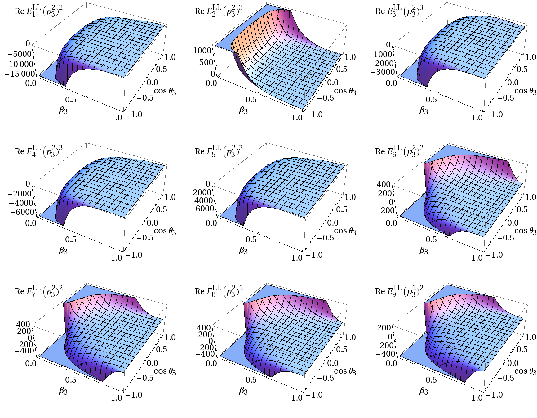
Figure 2: Real parts of the two loop form factors $E_{j}^{(2),LL\,[A]}$ for the process $gg\to V_{1}V_{2}$. The plots illustrate their dependence on the velocity, $\beta_{3}$, and the cosine of the scattering angle, $\cos\theta_{3}$, of the vector boson $V_{1}$, where $p_{4}^{2}=2p_{3}^{2}$ is chosen for the vector boson virtualities.

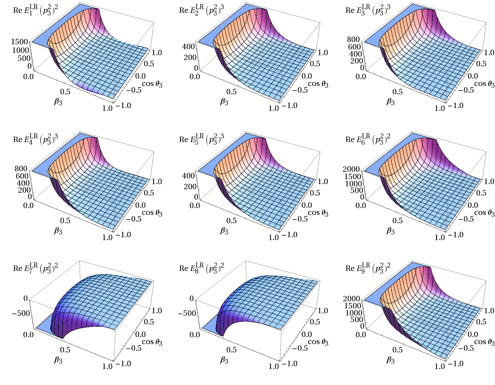
Figure 3: Real parts of the two loop form factors $E_{j}^{(2),LR\,[A]}$ for the process $gg\to V_{1}V_{2}$. The plots illustrate their dependence on the velocity, $\beta_{3}$, and the cosine of the scattering angle, $\cos\theta_{3}$, of the vector boson $V_{1}$, where $p_{4}^{2}=2p_{3}^{2}$ is chosen for the vector boson virtualities.

For the numerical evaluation of the helicity amplitudes for $gg\to V_{1}V_{2}\to 4~{}\mathrm{leptons}$, we implemented our results for the form factors $E_{j}^{\lambda_{1}\lambda_{2}\,[A]}$ and $A_{j}^{[A]}$ at one- and two-loop order in a dedicated C++ code. The implementation is based on the solutions for the master integrals presented in Gehrmann:2015ora , which were specifically constructed for fast and reliable numerical evaluations. We organised our form factor implementation in form of a library, which is supplemented by a simple command line interface. We provide the software package for public download on HepForge at http://vvamp.hepforge.org.

For the numerical evaluation of the multiple polylogarithms encountered in the solutions for the master integrals, we employ their implementation Vollinga:2004sn in the GiNaC Bauer:2000cp library. To identify and account for possible numerical instabilities of the form factors in collinear or other potentially problematic regions of phase space, the code compares numerical evaluations, which are obtained using different floating point data types, similar to the setup used in Gehrmann:2015ora . If the results obtained with different precision settings differ beyond a user-defined tolerance, the code successively increases the precision until the target precision is met.

For the rather central benchmark point of Caola:2014iua , the double precision mode of our code takes roughly $600ms$ on a single computer core and results in at least $11$ significant digits for all of the $E_{j}^{\lambda_{1}\lambda_{2}\,[A]}$. In order to estimate the actual precision, the default behaviour of our code is to reevaluate the algebraic expressions in quad precision, which results in a total run-time of roughly $3s$ for this phase space point. The run-time can increase further for regions close to the phase space boundaries, where the multiple polylogarithms take more time to evaluate and the precision control of our code may switch to higher precision computations in order to return reliable numbers. Depending on the precision setting and on the region of phase space, the evaluations of the multiple polylogarithms and of the algebraic coefficients may require comparable portions of the run-time. However, in double precision mode or close to the phase space boundaries, the run-time is dominated by multiple polylogarithm evaluations. The described version of our code implements a minimal set of $9$ coefficients $A_{j}$ and employs four evaluations of them with different kinematics in order to derive the remaining form factors using crossing relations. If required, it is straight-forward to further improve the evaluation speed, either by proper caching of multiple polylogarithms or, at the price of an increased code size, by an explicit implementation of all form factors, as we did for the process $q\bar{q}^{\prime}\to V_{1}V_{2}$ in Gehrmann:2015ora .

In order to illustrate the form factors and the reliability of the code, we used the latter to plot the real part of the two-loop form factors for the case $p_{4}^{2}=2p_{3}^{2}$ in Figures 2 and 3. In the plots, we vary the relativistic velocity $\beta_{3}$ and the cosine of the scattering angle $\cos\theta_{3}$ of the vector boson $V_{1}$, where $\beta_{3}=\kappa/(s+p_{3}^{2}-p_{4}^{2})$ and $\cos\theta_{3}=(2t+s-p_{3}^{2}-p_{4}^{2})/\kappa$. Compared to the results for the form factors $E_{j}$ in the process $q\bar{q}^{\prime}\to V_{1}V_{2}$ in Gehrmann:2015ora , we observe strong enhancements for the forward, backward and production threshold regions for the form factors in the present case. However, for the physical helicity amplitudes (40) we wish to point out that an additional dampening (very) close to the aforementioned phase space boundaries should be taken into account due to the additional overall factors $C_{LL}$ and $C_{LR}$ (41).

6 Conclusions

In this paper we computed the two-loop massless QCD corrections to the helicity amplitudes for the production of pairs of off-shell electroweak gauge bosons, $V_{1}V_{2}$, in the gluon fusion channel. For the calculation we employed the solutions for the master integrals presented in Gehrmann:2015ora . Contracting the diboson amplitude with the leptonic decay currents we have constructed the helicity amplitudes for $gg\to V_{1}V_{2}\to 4~{}\mathrm{leptons}$. We have compared our results to an independent calculation Caola:2015ila and find perfect agreement. Our results for these amplitudes provide the fundamental ingredient required to compute the NLO corrections to diboson production processes in gluon fusion. These corrections would contribute formally at N³LO to the processes $pp\to V_{1}V_{2}+X$, but their inclusion may be important to match the expected experimental accuracy due to the large gluon luminosity at the LHC. In particular studying their impact is required to obtain a more reliable estimate of the theory uncertainty and to establish more precise constraints on the total Higgs decay width Campbell:2011cu ; Caola:2013yja ; Campbell:2013una . We provide both analytical results and a C++ code for the numerical evaluation of the amplitudes on HepForge at http://vvamp.hepforge.org.

Appendix A Form factor relations

In this Appendix we present the explicit formulae needed in order to compute the $18$ form factors $E_{j}^{\lambda_{1}\lambda_{2}}$ defined for the amplitude (40), starting from the $20$ form factors $A_{j}$ defined in (13). For the $M_{LLLL}$ amplitude we find

$$E_{1}^{LL}=\frac{2A_{1}+A_{2}+A_{3}}{t\,u-p_{3}^{2}\,p_{4}^{2}}-\frac{A_{16}}{s}\,,$$

$$E_{2}^{LL}=\frac{A_{14}(t-p_{4}^{2})-A_{12}(u-p_{3}^{2})-s\,A_{4}}{s(t\,u-p_{3}^{2}\,p_{4}^{2})}+\frac{A_{17}}{2\,s}\,,$$

$$E_{3}^{LL}=\frac{A_{14}(u-p_{4}^{2})-A_{13}(u-p_{3}^{2})+A_{2}+A_{3}-s\,A_{5}}{s(t\,u-p_{3}^{2}\,p_{4}^{2})}+\frac{A_{18}}{2\,s}\,,$$

$$E_{4}^{LL}=\frac{A_{15}(t-p_{4}^{2})-A_{12}(t-p_{3}^{2})+A_{2}+A_{3}-s\,A_{6}}{s(t\,u-p_{3}^{2}\,p_{4}^{2})}+\frac{A_{19}}{2\,s}\,,$$

$$E_{5}^{LL}=\frac{A_{15}(u-p_{4}^{2})-A_{13}(t-p_{3}^{2})-s\,A_{7}}{s(t\,u-p_{3}^{2}\,p_{4}^{2})}+\frac{A_{20}}{2\,s}\,,$$

$$E_{6}^{LL}=\frac{(u-p_{3}^{2})(A_{2}-A_{3})}{s(t\,u-p_{3}^{2}\,p_{4}^{2})}+\frac{A_{10}-A_{14}}{s}\,,\qquad\quad E_{7}^{LL}=\frac{(t-p_{4}^{2})(A_{2}-A_{3})}{s(t\,u-p_{3}^{2}\,p_{4}^{2})}+\frac{A_{8}-A_{12}}{s}\,,$$

$$E_{8}^{LL}=\frac{(u-p_{4}^{2})(A_{2}-A_{3})}{s(t\,u-p_{3}^{2}\,p_{4}^{2})}+\frac{A_{9}-A_{13}}{s}\,,\qquad\quad\;E_{9}^{LL}=\frac{(t-p_{3}^{2})(A_{2}-A_{3})}{s(t\,u-p_{3}^{2}\,p_{4}^{2})}+\frac{A_{11}-A_{15}}{s}\,.$$ (59)

For the $M_{LRLL}$ amplitude we have instead

$$E_{1}^{LR} =\frac{A_{2}+A_{3}}{t\,u-p_{3}^{2}\,p_{4}^{2}}+\frac{A_{16}}{s}\,,\quad E_{2}^{LR} =-\frac{A_{17}}{2\,s}\,,$$

$$E_{3}^{LR} =\frac{A_{2}+A_{3}}{s(t\,u-p_{3}^{2}\,p_{4}^{2})}-\frac{A_{18}}{2\,s}\,, E_{4}^{LR} =\frac{A_{2}+A_{3}}{s(t\,u-p_{3}^{2}\,p_{4}^{2})}-\frac{A_{19}}{2\,s}\,,$$

$$E_{5}^{LR} =-\frac{A_{20}}{2\,s}\,, E_{6}^{LR} =\frac{(u-p_{3}^{2})(A_{2}+A_{3})}{s(t\,u-p_{3}^{2}\,p_{4}^{2})}-\frac{A_{10}+A_{14}}{s}\,,$$

$$E_{7}^{LR} =-\frac{(t-p_{4}^{2})(A_{2}+A_{3})}{s(t\,u-p_{3}^{2}\,p_{4}^{2})}-\frac{A_{8}+A_{12}}{s}\,, E_{8}^{LR} =-\frac{(u-p_{4}^{2})(A_{2}+A_{3})}{s(t\,u-p_{3}^{2}\,p_{4}^{2})}-\frac{A_{9}+A_{13}}{s}\,,$$

$$E_{9}^{LR} =\frac{(t-p_{3}^{2})(A_{2}+A_{3})}{s(t\,u-p_{3}^{2}\,p_{4}^{2})}-\frac{A_{11}+A_{15}}{s}\,.$$ (60)

Let us consider the behaviour of the form factors $E_{j}^{\lambda_{1}\lambda_{2}}$ under the two permutations $\pi_{12}$ and $\pi_{34}$ defined in (26). Using the crossing relations for the form factors $A_{j}^{[A]}$ (27) and (28) one easily finds the corresponding ones for the form factors $E_{j}^{\lambda_{1}\lambda_{2}\,{[A]}}$. To simplify our notation, we drop the superscript $[A]$ in the following. Under permutation $\pi_{12}$ we obtain

$$E^{LL}_{1}(s,u,p_{3}^{2},p_{4}^{2}) =E^{LL}_{1}(s,t,p_{3}^{2},p_{4}^{2})\,,$$

$$E^{LL}_{2}(s,u,p_{3}^{2},p_{4}^{2}) =E^{LL}_{5}(s,t,p_{3}^{2},p_{4}^{2})+\frac{(u-p_{4}^{2})E^{LL}_{9}(s,t,p_{3}^{2},p_{4}^{2})-(t-p_{3}^{2})E^{LL}_{8}(s,t,p_{3}^{2},p_{4}^{2})}{tu-p_{3}^{2}\,p_{4}^{2}}\,,$$

$$E^{LL}_{3}(s,u,p_{3}^{2},p_{4}^{2}) =E^{LL}_{4}(s,t,p_{3}^{2},p_{4}^{2})+\frac{(t-p_{4}^{2})E^{LL}_{9}(s,t,p_{3}^{2},p_{4}^{2})-(t-p_{3}^{2})E^{LL}_{7}(s,t,p_{3}^{2},p_{4}^{2})}{tu-p_{3}^{2}\,p_{4}^{2}}\,,$$

$$E^{LL}_{6}(s,u,p_{3}^{2},p_{4}^{2}) =-E^{LL}_{9}(s,t,p_{3}^{2},p_{4}^{2})\,,\qquad\;\;\;E^{LL}_{7}(s,u,p_{3}^{2},p_{4}^{2})=-E^{LL}_{8}(s,t,p_{3}^{2},p_{4}^{2})$$ (61)

and

$$E^{LR}_{1}(s,u,p_{3}^{2},p_{4}^{2}) =E^{LR}_{1}(s,t,p_{3}^{2},p_{4}^{2})\,,\qquad\;\;\,\, E^{LR}_{2}(s,u,p_{3}^{2},p_{4}^{2}) =E^{LR}_{5}(s,t,p_{3}^{2},p_{4}^{2})\,,\qquad\phantom{=}$$

$$E^{LR}_{3}(s,u,p_{3}^{2},p_{4}^{2}) =E^{LR}_{4}(s,t,p_{3}^{2},p_{4}^{2})\,, E^{LR}_{6}(s,u,p_{3}^{2},p_{4}^{2}) =E^{LR}_{9}(s,t,p_{3}^{2},p_{4}^{2})\,,$$

$$E^{LR}_{7}(s,u,p_{3}^{2},p_{4}^{2}) =E^{LR}_{8}(s,t,p_{3}^{2},p_{4}^{2})\,.$$ (62)

Under permutation $\pi_{34}$, instead, the form factors for both the $LL$ and $LR$ helicity configurations transform in the same way

$$E^{\lambda_{1}\lambda_{2}}_{1}(s,u,p_{4}^{2},p_{3}^{2}) =E^{\lambda_{1}\lambda_{2}}_{1}(s,t,p_{3}^{2},p_{4}^{2})\,,\quad\;\; E^{\lambda_{1}\lambda_{2}}_{2}(s,u,p_{4}^{2},p_{3}^{2}) =E^{\lambda_{1}\lambda_{2}}_{2}(s,t,p_{3}^{2},p_{4}^{2})\,,$$

$$E^{\lambda_{1}\lambda_{2}}_{3}(s,u,p_{4}^{2},p_{3}^{2}) =E^{\lambda_{1}\lambda_{2}}_{4}(s,t,p_{3}^{2},p_{4}^{2})\,, E^{\lambda_{1}\lambda_{2}}_{5}(s,u,p_{4}^{2},p_{3}^{2}) =E^{\lambda_{1}\lambda_{2}}_{5}(s,t,p_{3}^{2},p_{4}^{2})\,,$$

$$E^{\lambda_{1}\lambda_{2}}_{6}(s,u,p_{4}^{2},p_{3}^{2}) =-E^{\lambda_{1}\lambda_{2}}_{7}(s,t,p_{3}^{2},p_{4}^{2})\,, E^{\lambda_{1}\lambda_{2}}_{8}(s,u,p_{4}^{2},p_{3}^{2}) =-E^{\lambda_{1}\lambda_{2}}_{9}(s,t,p_{3}^{2},p_{4}^{2})\,.$$ (63)

Exploiting all of these crossing relations we find that only $9$ out of the $18$ form factors $E_{j}^{\lambda_{1}\lambda_{2}}$ are effectively independent, while the other $9$ can be obtained by the crossing rules above. The number of independent form factors $E_{j}^{\lambda_{1}\lambda_{2}}$ coincides with the number of independent form factors $A_{j}$ found in Section 2.

References

• (1) S. Catani, L. Cieri, D. de Florian, G. Ferrera, and M. Grazzini, Diphoton production at hadron colliders: a fully-differential QCD calculation at NNLO, Phys.Rev.Lett. 108 (2012) 072001, [arXiv:1110.2375].
• (2) M. Grazzini, S. Kallweit, D. Rathlev, and A. Torre, $Z\gamma$ production at hadron colliders in NNLO QCD, Phys.Lett. B731 (2014) 204, [arXiv:1309.7000].
• (3) F. Cascioli, T. Gehrmann, M. Grazzini, S. Kallweit, P. Maierhöfer, A. von Manteuffel, S. Pozzorini, D. Rathlev, and L. Tancredi, ZZ production at hadron colliders in NNLO QCD, Phys.Lett. B735 (2014) 311–313, [arXiv:1405.2219].
• (4) T. Gehrmann, M. Grazzini, S. Kallweit, P. Maierhöfer, A. von Manteuffel, S. Pozzorini, D. Rathlev, and L. Tancredi, $W^{+}W^{-}$ Production at Hadron Colliders in Next to Next to Leading Order QCD, Phys.Rev.Lett. 113 (2014) 212001, [arXiv:1408.5243].
• (5) C. Anastasiou, J. Cancino, F. Chavez, C. Duhr, A. Lazopoulos, B. Mistlberger, and R. Müller, NNLO QCD corrections to pp $\to$ $\gamma^{*}\gamma^{*}$ in the large NF limit, JHEP 1502 (2015) 182, [arXiv:1408.4546].
• (6) V. Costantini, B. De Tollis, and G. Pistoni, Nonlinear effects in quantum electrodynamics, Nuovo Cim. A2 (1971) 733–787.
• (7) J. van der Bij and E. N. Glover, Photon Z Boson Pair Production via Gluon Fusion, Phys.Lett. B206 (1988) 701.
• (8) E. W. N. Glover and J. van der Bij, Z Boson Pair Production via Gluon Fusion, Nucl.Phys. B321 (1989) 561.
• (9) E. N. Glover and J. van der Bij, Vector Boson Pair Production via Gluon Fusion, Phys.Lett. B219 (1989) 488.
• (10) K. Adamson, D. de Florian, and A. Signer, Gluon induced contributions to WZ and W gamma production at NNLO, Phys.Rev. D65 (2002) 094041, [hep-ph/0202132].
• (11) K. Adamson, D. de Florian, and A. Signer, Gluon induced contributions to $Z\gamma$ production at hadron colliders, Phys.Rev. D67 (2003) 034016, [hep-ph/0211295].
• (12) T. Binoth, M. Ciccolini, N. Kauer, and M. Kramer, Gluon-induced W-boson pair production at the LHC, JHEP 0612 (2006) 046, [hep-ph/0611170].
• (13) T. Binoth, M. Ciccolini, N. Kauer, and M. Kramer, Gluon-induced WW background to Higgs boson searches at the LHC, JHEP 0503 (2005) 065, [hep-ph/0503094].
• (14) F. Cascioli, S. Hoche, F. Krauss, P. Maierhofer, S. Pozzorini, et al., Precise Higgs-background predictions: merging NLO QCD and squared quark-loop corrections to four-lepton + 0,1 jet production, JHEP 1401 (2014) 046, [arXiv:1309.0500].
• (15) S. Dawson, Radiative corrections to Higgs boson production, Nucl.Phys. B359 (1991) 283–300.
• (16) A. Djouadi, M. Spira, and P. Zerwas, Production of Higgs bosons in proton colliders: QCD corrections, Phys.Lett. B264 (1991) 440–446.
• (17) M. Spira, A. Djouadi, D. Graudenz, and P. Zerwas, Higgs boson production at the LHC, Nucl.Phys. B453 (1995) 17–82, [hep-ph/9504378].
• (18) Z. Bern, A. De Freitas, and L. J. Dixon, Two loop amplitudes for gluon fusion into two photons, JHEP 0109 (2001) 037, [hep-ph/0109078].
• (19) Z. Bern, L. J. Dixon, and C. Schmidt, Isolating a light Higgs boson from the diphoton background at the CERN LHC, Phys.Rev. D66 (2002) 074018, [hep-ph/0206194].
• (20) J. M. Campbell, R. K. Ellis, and C. Williams, Gluon-Gluon Contributions to W+ W- Production and Higgs Interference Effects, JHEP 1110 (2011) 005, [arXiv:1107.5569].
• (21) N. Kauer and G. Passarino, Inadequacy of zero-width approximation for a light Higgs boson signal, JHEP 1208 (2012) 116, [arXiv:1206.4803].
• (22) F. Caola and K. Melnikov, Constraining the Higgs boson width with ZZ production at the LHC, Phys.Rev. D88 (2013) 054024, [arXiv:1307.4935].
• (23) J. M. Campbell, R. K. Ellis, and C. Williams, Bounding the Higgs width at the LHC using full analytic results for $gg->e^{-}e^{+}\mu^{-}\mu^{+}$, JHEP 1404 (2014) 060, [arXiv:1311.3589].
• (24) C. Berger, Z. Bern, L. Dixon, F. Febres Cordero, D. Forde, H. Ita, D. Kosower, and D. Maître, An Automated Implementation of On-Shell Methods for One-Loop Amplitudes, Phys.Rev. D78 (2008) 036003, [arXiv:0803.4180].
• (25) V. Hirschi, R. Frederix, S. Frixione, M. V. Garzelli, F. Maltoni, and R. Pittau, Automation of one-loop QCD corrections, JHEP 1105 (2011) 044, [arXiv:1103.0621].
• (26) R. K. Ellis, Z. Kunszt, K. Melnikov, and G. Zanderighi, One-loop calculations in quantum field theory: from Feynman diagrams to unitarity cuts, Phys.Rept. 518 (2012) 141–250, [arXiv:1105.4319].
• (27) G. Bevilacqua, M. Czakon, M. Garzelli, A. van Hameren, A. Kardos, C. Papadopoulos, R. Pittau, and M. Worek, HELAC-NLO, Comput.Phys.Commun. 184 (2013) 986–997, [arXiv:1110.1499].
• (28) G. Cullen, N. Greiner, G. Heinrich, G. Luisoni, P. Mastrolia, G. Ossola, T. Reiter, and F. Tramontano, Automated One-Loop Calculations with GoSam, Eur.Phys.J. C72 (2012) 1889, [arXiv:1111.2034].
• (29) F. Cascioli, P. Maierhofer, and S. Pozzorini, Scattering Amplitudes with Open Loops, Phys.Rev.Lett. 108 (2012) 111601, [arXiv:1111.5206].
• (30) G. Cullen, H. van Deurzen, N. Greiner, G. Heinrich, G. Luisoni, P. Mastrolia, E. Mirabella, G. Ossola, T. Peraro, J. Schlenk, J. von Soden-Fraunhofen, and F. Tramontano, G$\scriptsize{O}$S$\scriptsize{AM}$-2.0: a tool for automated one-loop calculations within the Standard Model and beyond, Eur.Phys.J. C74 (2014), no. 8 3001, [arXiv:1404.7096].
• (31) T. Gehrmann, L. Tancredi, and E. Weihs, Two-loop QCD helicity amplitudes for $g\,g\to Z\,g$ and $g\,g\to Z\,\gamma$, JHEP 1304 (2013) 101, [arXiv:1302.2630].
• (32) S. Frixione, Z. Kunszt, and A. Signer, Three jet cross-sections to next-to-leading order, Nucl.Phys. B467 (1996) 399–442, [hep-ph/9512328].
• (33) S. Catani and M. Seymour, A General algorithm for calculating jet cross-sections in NLO QCD, Nucl.Phys. B485 (1997) 291–419, [hep-ph/9605323].
• (34) T. Gehrmann, L. Tancredi, and E. Weihs, Two-loop master integrals for $q\bar{q}\to VV$: the planar topologies, JHEP 1308 (2013) 070, [arXiv:1306.6344].
• (35) T. Gehrmann, A. von Manteuffel, L. Tancredi, and E. Weihs, The two-loop master integrals for $q\bar{q}\to VV$, JHEP 1406 (2014) 032, [arXiv:1404.4853].
• (36) J. M. Henn, K. Melnikov, and V. A. Smirnov, Two-loop planar master integrals for the production of off-shell vector bosons in hadron collisions, JHEP 1405 (2014) 090, [arXiv:1402.7078].
• (37) F. Caola, J. M. Henn, K. Melnikov, and V. A. Smirnov, Non-planar master integrals for the production of two off-shell vector bosons in collisions of massless partons, JHEP 1409 (2014) 043, [arXiv:1404.5590v2].
• (38) C. G. Papadopoulos, D. Tommasini, and C. Wever, Two-loop Master Integrals with the Simplified Differential Equations approach, JHEP 1501 (2015) 072, [arXiv:1409.6114].
• (39) T. Gehrmann, A. von Manteuffel, and L. Tancredi, The two-loop helicity amplitudes for $q\bar{q}^{\prime}\to V_{1}V_{2}\to 4~{}\mathrm{leptons}$, arXiv:1503.04812.
• (40) F. Caola, J. M. Henn, K. Melnikov, A. V. Smirnov, and V. A. Smirnov, Two-loop helicity amplitudes for the production of two off-shell electroweak bosons in quark-antiquark collisions, JHEP 1411 (2014) 041, [arXiv:1408.6409].
• (41) F. Chavez and C. Duhr, Three-mass triangle integrals and single-valued polylogarithms, JHEP 1211 (2012) 114, [arXiv:1209.2722].
• (42) K. Melnikov and M. Dowling, Production of two Z-bosons in gluon fusion in the heavy top quark approximation, arXiv:1503.01274.
• (43) A. Denner, Techniques for calculation of electroweak radiative corrections at the one loop level and results for W physics at LEP-200, Fortsch.Phys. 41 (1993) 307–420, [arXiv:0709.1075].
• (44) L. J. Dixon, Calculating scattering amplitudes efficiently, hep-ph/9601359.
• (45) L. J. Dixon, Z. Kunszt, and A. Signer, Helicity amplitudes for O($\alpha_{s}$) production of $W^{+}W^{-}$, $W^{\pm}Z$, $ZZ$, $W^{\pm}\gamma$, or $Z\gamma$ pairs at hadron colliders, Nucl.Phys. B531 (1998) 3–23, [hep-ph/9803250].
• (46) P. Nogueira, Automatic Feynman graph generation, J.Comput.Phys. 105 (1993) 279–289.
• (47) F. Tkachov, A Theorem on Analytical Calculability of Four Loop Renormalization Group Functions, Phys.Lett. B100 (1981) 65–68.
• (48) K. Chetyrkin and F. Tkachov, Integration by Parts: The Algorithm to Calculate beta Functions in 4 Loops, Nucl.Phys. B192 (1981) 159–204.
• (49) T. Gehrmann and E. Remiddi, Differential equations for two loop four point functions, Nucl.Phys. B580 (2000) 485–518, [hep-ph/9912329].
• (50) S. Laporta, High precision calculation of multiloop Feynman integrals by difference equations, Int.J.Mod.Phys. A15 (2000) 5087–5159, [hep-ph/0102033].
• (51) A. von Manteuffel and C. Studerus, Reduze 2 - Distributed Feynman Integral Reduction, arXiv:1201.4330.
• (52) C. Studerus, Reduze-Feynman Integral Reduction in C++, Comput.Phys.Commun. 181 (2010) 1293–1300, [arXiv:0912.2546].
• (53) C. W. Bauer, A. Frink, and R. Kreckel, Introduction to the GiNaC framework for symbolic computation within the C++ programming language, J.Symb.Comput. 33 (2002) 1–12, [cs/0004015].
• (54) R. Lewis, Computer Algebra System Fermat. http://www.bway.net/~lewis.
• (55) J. Vermaseren, New features of FORM, math-ph/0010025.
• (56) S. Catani, The Singular behavior of QCD amplitudes at two loop order, Phys.Lett. B427 (1998) 161–171, [hep-ph/9802439].
• (57) S. Catani, L. Cieri, D. de Florian, G. Ferrera, and M. Grazzini, Universality of transverse-momentum resummation and hard factors at the NNLO, Nucl.Phys. B881 (2014) 414–443, [arXiv:1311.1654].
• (58) F. Caola, J. M. Henn, K. Melnikov, A. V. Smirnov, and V. A. Smirnov, Two-loop helicity amplitudes for the production of two off-shell electroweak bosons in gluon fusion, arXiv:1503.08759.
• (59) J. Vollinga and S. Weinzierl, Numerical evaluation of multiple polylogarithms, Comput.Phys.Commun. 167 (2005) 177, [hep-ph/0410259].
• (60) D. Binosi and L. Theussl, JaxoDraw: A Graphical user interface for drawing Feynman diagrams, Comput.Phys.Commun. 161 (2004) 76–86, [hep-ph/0309015].
• (61) J. Vermaseren, Axodraw, Comput.Phys.Commun. 83 (1994) 45–58.