Swift J201424.9+152930: discovery of a new deeply eclipsing binary with 491-s and 3.4-h modulations

Abstract

We report on the discovery of a new X-ray pulsator, Swift J201424.9+152930 (Sw J2014). Owing to its X-ray modulation at 491 s, it was discovered in a systematic search for coherent signals in the archival data of the Swift X-ray Telescope. To investigate the nature of Sw J2014, we performed multi-wavelength follow-up observations with space-borne (Swift and XMM–Newton) and ground-based (the 1.5-m Loiano Telescope and the 3.6-m Telescopio Nazionale Galileo) instruments. The X-ray spectrum of Sw J2014 can be described by a hard and highly absorbed ($N_{\rm H}\sim 5\times 10^{22}$ cm^-2) power law ($\Gamma\sim 1$). The optical observations made it possible to single out the optical counterpart to this source, which displays several variable emission lines and total eclipses lasting $\approx$20 min. Total eclipses of similar length were observed also in X-rays. The study of the eclipses, allowed us to infer a second periodicity of 3.44 h, which we interpret as the orbital period of a close binary system. We also found that the period has not significantly changed over a $\sim$7 yr timespan. Based on the timing signatures of Sw J2014, and its optical and X-ray spectral properties, we suggest that it is a close binary hosting an accreting magnetic white dwarf. The system is therefore a cataclysmic variable of the intermediate polar type and one of the very few showing deep eclipses.

1 Introduction

Temporal investigation is crucial to properly identify the nature of an X-ray source or, at least, to significantly constrain it. For example, the discovery of type I (thermonuclear) X-ray bursts in a binary system securely identifies the compact object as a neutron star (NS), while the detection of fast X-ray pulsations rules out a black hole. In particular, timing analysis aimed at detecting periodic signals is one of the most powerful tools to pin down the nature of a source. For this reason, we have been working for years at systematic searches for coherent or quasi-coherent signals in the archival data of the Chandra (Weisskopf et al., 2002) and Swift (Gehrels et al., 2004) missions. These projects, the Chandra ACIS Timing Survey at Brera And Rome astronomical observatories (CATS @ BAR) and the Swift Automatic Timing Survey at Brera And Roma astronomical observatories (SATS @ BAR, formerly known as SATANASS @ BAR) have led so far to the discovery of about 40 new X-ray periodicities. Also taking advantage of optical observations, we have been able to securely classify the nature of several of these pulsators (see Esposito et al. 2013b, c, a, 2014).

In this paper we present a detailed study of the data of the X-ray point source Swift J201424.9+152930 (Sw J2014), which was serendipitously imaged during Swift followup observations of the gamma-ray burst GRB 061122 (Götz et al., 2013). During a run of the SATS @ BAR pipeline (see Section 2.4 for more details), we found a statistically significant periodicity in its X-ray emission, at $\sim$491 s. To investigate the nature of Sw J2014, we obtained further Swift and new XMM–Newton data, as well as optical (photometric and spectroscopic) observations with the Cassini telescope in Loiano and the Telescopio Nazionale Galileo (TNG) telescope in La Palma. In Sections 2, 3, and 4 we present the data and the results from their analysis, in Section 5 we discuss the nature of the source. A summary follows in Section 6.

2 Swift and XMM–Newton

2.1 Swift observations and data reduction

Sw J2014 was discovered in a series of 14 Swift observations devoted to GRB 061122 (target ID 20044), which were carried out in 2006 November through December. In these pointings, the source was generally $\sim$11^′ from the aim point of the X-Ray Telescope (XRT; Burrows et al. 2005) and the average exposure was $\sim$12.8 ks. In Table 1, we give a summary of these Swift observations, except for observations 4001 (where Sw J2014 was outside the field of view) and 4009 (where it was at the very edge of the detector), which were not used for this work. Additional Swift observations pointed at Sw J2014 (target ID 46265) were performed between 2011 December and 2013 December (see Table 1). Most of these observations were taken at the end of 2013, and have typical exposure of 9–10 ks each.

Each XRT data set was calibrated, filtered and screened according to standard criteria using xrtpipeline within the xrtdas package, included in the HEAsoft distribution v6.15. At the same time, exposure maps were produced for all observations. The X-ray source counts for the spectral and timing analysis were accumulated in circles centred on Sw J2014 and with radii from $\sim$30^′′ to 47^′′, depending on the off-axis distance, while the background was estimated from neighbouring, source-free regions. Since in the individual observations the count statistics were not enough to allow us a reasonable number of spectral bins, we created two combined spectra: one by merging the 2006 observations (total exposure 153.0 ks, about 1000 net source counts) and one from the 2013 November–December observations (5011–5037, total exposure 169.1 ks, about 1100 net source counts).

Table 1: Summary of the Swift and XMM–Newton X-ray observations of Sw J2014.

Obs. ID	Start	Stop	Net exposure	Count ratea
	(YYYY-MM-DD hh-mm-ss)		(ks)	(counts s-1)
Swift/XRT 00020044002	2006-11-23 01:37:55	2006-11-24 22:47:56	16.0	$(9.5\pm 1.4)\times 10^{-3}$
Swift/XRT 00020044003	2006-11-25 00:14:53	2006-11-25 22:58:58	14.2	$(6.9\pm 1.2)\times 10^{-3}$
Swift/XRT 00020044004	2006-11-26 00:22:02	2006-11-26 22:57:56	10.6	$(10.7\pm 1.9)\times 10^{-3}$
Swift/XRT 00020044005	2006-11-27 00:27:53	2006-11-27 23:15:57	12.9	$(9.7\pm 1.5)\times 10^{-3}$
Swift/XRT 00020044006	2006-11-28 00:32:54	2006-11-28 23:16:57	15.5	$(4.5\pm 0.9)\times 10^{-3}$
Swift/XRT 00020044007	2006-11-29 00:37:57	2006-11-29 23:25:58	16.0	$(11.9\pm 1.3)\times 10^{-3}$
Swift/XRT 00020044008	2006-11-30 00:45:18	2006-11-30 23:37:56	17.0	$(11.8\pm 1.3)\times 10^{-3}$
Swift/XRT 00020044010	2006-12-02 10:34:55	2006-12-03 02:46:38	7.8	$(10.1\pm 1.8)\times 10^{-3}$
Swift/XRT 00020044011	2006-12-03 04:14:54	2006-12-04 01:31:25	8.7	$(1.3\pm 0.2)\times 10^{-2}$
Swift/XRT 00020044012	2006-12-04 05:57:54	2006-12-04 23:59:56	10.7	$(11.2\pm 1.6)\times 10^{-3}$
Swift/XRT 00020044013	2006-12-05 01:18:07	2006-12-05 23:59:56	13.2	$(1.6\pm 0.2)\times 10^{-2}$
Swift/XRT 00020044014	2006-12-06 01:20:57	2006-12-06 23:59:56	11.1	$(11.1\pm 1.6)\times 10^{-3}$
Swift/XRT 00046265001	2011-12-26 21:01:46	2011-12-26 21:06:59	0.3	$<$$4.8\times 10^{-2}$
Swift/XRT 00046265002	2012-08-27 09:04:28	2012-08-27 09:08:53	0.3	$<$$6.2\times 10^{-2}$
Swift/XRT 00046265003	2012-09-24 21:42:36	2012-09-24 23:28:54	1.0	$(1.1\pm 0.4)\times 10^{-2}$
Swift/XRT 00046265004	2012-12-26 01:51:34	2012-12-26 23:10:55	3.9	$(4.7\pm 1.5)\times 10^{-3}$
Swift/XRT 00046265005	2013-03-08 04:52:49	2013-03-08 11:16:54	0.2	$<$$6.3\times 10^{-2}$
Swift/XRT 00046265007	2013-03-15 00:24:59	2013-03-16 13:24:55	8.7	$(2.0\pm 0.2)\times 10^{-2}$
Swift/XRT 00046265008	2013-03-18 09:55:58	2013-03-18 15:07:56	1.8	$(4.9\pm 2.3)\times 10^{-3}$
Swift/XRT 00046265009	2013-07-02 12:41:02	2013-07-02 12:45:55	0.3	$<$$5.2\times 10^{-2}$
Swift/XRT 00046265010	2013-09-16 02:11:05	2013-09-16 02:17:53	0.4	$<$$2.8\times 10^{-2}$
Swift/XRT 00046265011	2013-11-27 01:51:25	2013-11-27 22:51:55	8.9	$(14.0\pm 1.7)\times 10^{-3}$
Swift/XRT 00046265012	2013-11-28 00:12:26	2013-11-28 10:19:55	9.7	$(15.8\pm 1.7)\times 10^{-3}$
Swift/XRT 00046265013	2013-11-29 00:14:40	2013-11-29 14:46:56	9.5	$(9.6\pm 1.5)\times 10^{-3}$
Swift/XRT 00046265014	2013-11-30 00:15:40	2013-11-30 14:46:56	8.6	$(3.8\pm 0.9)\times 10^{-3}$
Swift/XRT 00046265015	2013-12-01 00:14:30	2013-12-01 14:48:56	9.6	$(5.3\pm 1.0)\times 10^{-3}$
Swift/XRT 00046265016	2013-12-02 00:15:02	2013-12-02 14:47:54	9.7	$(6.1\pm 1.1)\times 10^{-3}$
Swift/XRT 00046265018	2013-12-03 01:53:39	2013-12-03 16:26:57	9.4	$(6.4\pm 1.1)\times 10^{-3}$
Swift/XRT 00046265020	2013-12-04 00:17:55	2013-12-04 16:34:54	9.8	$(9.6\pm 1.4)\times 10^{-3}$
Swift/XRT 00046265024	2013-12-06 00:20:39	2013-12-06 12:05:54	9.6	$(15.5\pm 1.7)\times 10^{-3}$
Swift/XRT 00046265025	2013-12-07 00:23:36	2013-12-07 11:49:56	9.7	$(5.4\pm 1.0)\times 10^{-3}$
Swift/XRT 00046265027	2013-12-08 00:21:12	2013-12-08 16:25:55	9.6	$(3.3\pm 0.8)\times 10^{-3}$
Swift/XRT 00046265028	2013-12-09 00:26:36	2013-12-09 13:29:54	9.6	$(5.9\pm 1.1)\times 10^{-3}$
Swift/XRT 00046265030	2013-12-10 08:25:39	2013-12-10 22:57:54	9.9	$(4.0\pm 0.8)\times 10^{-3}$
Swift/XRT 00046265032	2013-12-11 03:38:36	2013-12-11 19:49:55	9.5	$(5.6\pm 1.1)\times 10^{-3}$
Swift/XRT 00046265034	2013-12-12 00:32:54	2013-12-12 18:14:56	9.4	$(6.1\pm 1.1)\times 10^{-3}$
Swift/XRT 00046265036	2013-12-13 00:30:44	2013-12-13 19:57:54	9.3	$(9.2\pm 1.4)\times 10^{-3}$
Swift/XRT 00046265037	2013-12-14 00:32:04	2013-12-14 23:09:55	9.3	$(16.6\pm 1.9)\times 10^{-3}$
XMM–Newton/EPIC 0743980501 (pn)	2014-05-02 11:58:12	2014-05-02 17:25:23	16.7	$0.105\pm 0.005$
XMM–Newton/EPIC 0743980501 (MOS 1)	2014-05-02 11:35:27	2014-05-02 17:20:43	20.5	$0.022\pm 0.002$
XMM–Newton/EPIC 0743980501 (MOS 2)	2014-05-02 11:36:00	2014-05-02 17:20:55	20.5	$0.032\pm 0.002$

• Net source count rate in the 0.3–10 keV band; when the source is not detected, a 3$\sigma$ upper limit is given.

Sw J2014 was in the Ultra-Violet/Optical Telescope (UVOT; Roming et al. 2005) field of view only in the observations pointed to the source (target ID 46265). The data were collected in imaging mode in near ultraviolet (UV), with the filters $uw1$ (central wavelength 2600 Å, FWHM 693 Å), $um2$ (2246 Å, FWHM 498 Å), and $uw2$ (1928 Å, FWHM 657 Å). The analysis was performed for each filter on the stacked images of the individual observations with the uvotsource task, which calculates count rates, flux densities and magnitudes through aperture photometry within a circular region and applies specific corrections due to the detector characteristics. Since Sw J2014 is in a crowded field (see Section 4), we adopted an extraction radius of 3 arcsec and applied the corresponding aperture corrections.

2.2 XMM–Newton observations and data reduction

XMM–Newton observed Sw J2014 on 2014 May 02 for approximately 21 ks (Obs. ID: 0743980501). The EPIC pn (Strüder et al., 2001) and MOS (Turner et al., 2001) detectors were set in Full Frame mode and used the Medium optical blocking filter. The OM telescope (Mason et al., 2001) was operated in Fast mode and the $B$ filter (390–490 nm) was used during the observation for all exposures. The exposure time was 19.6 ks for the pn (16.7 ks net exposure) and 20.7 ks for the MOS 1 and MOS 2 (20.5 ks net exposure). Seven OM exposures were scheduled, of duration 1.0, 4.4, 4.4, 4.0, 1.2, 4.0, and 1.2 ks; however, due to a problem with the data processing unit (DPU), the OM data of the first three exposures were lost and the OM data started $\sim$10 ks after the EPIC ones, for a total exposure time of $\sim$10.4 ks.

The raw observation EPIC data files were processed with the XMM–Newton Science Analysis Software (sas, v.13.5) using standard pipeline tasks, epproc and emproc for the pn and MOSs, respectively. Likewise, the OM data were processed with the sas omfchain pipeline and the Sw J2014’s light curves were binned in 20-s intervals. Standard screening criteria were applied.

The X-ray data were affected by very strong soft-proton flares, in particular during the second half of the exposure. For the spectral analysis, we removed the intervals of flaring background with a 3$\sigma$ clipping filter. This resulted in a net exposure time of 7.8 ks in the pn, 11.3 ks in the MOS 1, and 11.5 ks in the MOS 2. For the timing analysis, since the same procedure would significantly alter the time series, we choose instead to dynamically subtract the scaled background in each bin of the source light curves binned at 10 s.

2.3 X-ray position

Figure 1: Swift and XMM–Newton folded light curves (491-s modulation, background-subtracted). Each data set was folded at its best period and the profiles have been aligned so that the minimum bin coincides with phase 0.

In X-rays, due to the larger number of collected photons, XMM–Newton offers much better positional accuracy with respect to Swift/XRT. Based on the combined pn and MOS images, the emldetect routine reports for Sw J2014 the best-fitting position (J2000) $\rm RA=20^{h}14^{m}24\aas@@fstack{s}96,~{}Decl.=+15\degr 29^{\prime}29\aas@@fstack{\prime\prime}04$, with a statistical uncertainty of $0\aas@@fstack{\prime\prime}2$ (radius; here and in the following all uncertainties are at 1$\sigma$ confidence level). This is much smaller than the absolute astrometric accuracy of XMM–Newton, $1\aas@@fstack{\prime\prime}5$ root mean square (Kirsch et al., 2004), which is thus a more realistic indication of the actual uncertainty. About 20 other weak X-ray sources are present in the EPIC images (they are all fainter than Sw J2014 and none is closer than 2.4 arcmin to it) but, since they have no obvious and unambiguous optical or infrared counterparts, it was not possible to use them to improve the XMM–Newton absolute astrometry.

In all the optical data that we will discuss in the following, there is always only a single source consistent with the X-ray position of Sw J2014. Thus, we identify that source (see Section 4) as the counterpart of Sw J2014. Finally, we note that this optical counterpart is consistent with the NOMAD source 1054-0592809 ($B\sim 19.3$ mag, $R\sim 18.9$ mag, 1050–16948097 in the USNO-A2 catalog and 1054–0559015 in the USNO-B1 catalogue, see also Section 4).

2.4 Timing analysis

The $\sim$491-s signal from Sw J2014 was first detected within the SATS @ BAR project. SATS @ BAR consists in a systematic Fourier-based search for new pulsators in the archival Swift X-ray data. So far, about 4000 XRT light curves of point sources with a sufficiently high number of photons ($\ga$150) were analysed and the effort yielded six previously unknown X-ray pulsators (including Sw J2014, while three further new X-ray pulsators were reported in Nichelli et al. 2009 and Esposito et al. 2014).

The original detection of the period of Sw J2014 occurred in the piled Swift 2006 observations (see Table 1). The significance of the signal (as inferred from the automatic analysis and normalized for the number of searched frequencies and light curves) was above the a priori threshold of about 4$\sigma$. By a standard phase-fitting analysis, the value of the period was refined to $P=491.26(1)$ s.

After that, more Swift observations were carried out, in particular in late 2013. The period measured during the latest Swift campaign, using the observation from 2013 November 27 to December 14, $P=491.27(2)$ s, is consistent with that inferred in the 2006 observations. In our recent XMM–Newton observation, executed on 2014 May 02, the period was $P=491(1)$ s, which is again consistent, albeit within a comparatively large error, with the previous measures. The 3$\sigma$ limit on the period derivative drawn from these measures by a linear fit is $-2.6\times 10^{-10}~{}\mathrm{s~{}s}^{-1}<\dot{P}<3.5\times 10^{-10}~{}\mathrm{s~{}s}^{-1}$. The long-term stability of the period suggests that the periodic modulation is originated by the spin of a compact object, likely a white dwarf (WD; due to its larger momentum of inertia, a WD is much harder than an NS to spin-up or spin-down, see e.g. Patterson 1994; Bildsten et al. 1997; Frank et al. 2002), or by the revolution of two rather close compact objects.

The pulse profiles are shown in Fig. 1. The pulsed fractions, measured with a sine-wave fit, were $48\pm 5$% in the 2006 Swift data, $50\pm 5$% in the 2013 Swift data, and $44\pm 5$% in the XMM–Newton data. The data suggest a trend of pulsed fraction decreasing with energy. However, it is not statistically significant, since the values are compatible within the uncertainties. For example, in the XMM–Newton data, the pulsed fraction is $47\pm 8$% in the soft ($<$3 keV) band and $36\pm 4$% in the hard ($>$3 keV) band. We also computed hardness ratios between profiles in a number of different energy bands (including the soft and hard band mentioned above), but no statistically significant deviation from the average ratio were observed along the 491-s cycle. We searched also the XMM–Newton/OM optical data for the 491-s periodicity by a Fourier transform, as well as by a folding analysis around the X-ray period. No statistically significant signal could be found. The 3$\sigma$ upper limit of the pulsed fraction, computed following Vaughan et al. (1994), is 10% for a sinusoidal signal. Finally, we notice that, although the pulse profiles (and the hardness ratios) obtained by folding the Swift and XMM–Newton data of Sw J2014 at the double of the period are rather symmetrical, we cannot exclude that the true period of the source is $\sim$982 s.

2.4.1 Eclipses and second (orbital) period

The inspection of the EPIC (pn + MOSs) and OM light curves clearly revealed two overall similar broad features, one in each instrument data set (Fig. 2). In both instances, in a few hundreds of seconds the source flux suddenly decreased to a flux level consistent with zero and quickly recovered (to the pre-event flux level in the case of the EPIC data, while the last part of the optical eclipse was not observed by the OM). These properties are reminiscent of the total eclipses in low-mass X-ray binaries with an accreting NS or cataclysmic variables (CVs).

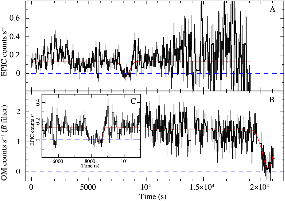
Figure 2: XMM–Newton pn and OM light curves. In panels A and B, the red solid line indicates the constant-plus-Gaussian model used to infer the time and the duration of the eclipse. In inset C, we show a close-up of the X-ray eclipse, and the red line represents the piecewise linear model fit to the data.

To determine the epoch and duration of the eclipses, we modelled the data with Gaussian functions. The EPIC eclipse occurred at MJD 56 779.6265(6) (Barycentric Dynamical Time (TDB), centre of the event) and could be modelled by a Gaussian with $\sigma=344\pm 52$ s (FWHM duration: $809\pm 122$ s). The OM eclipse took place at MJD 56 779.771(1) (TDB) and could be modelled by a Gaussian with $\sigma=493\pm 141$ s (FWHM duration: $1160\pm 332$ s; but again we note that the OM coverage of the event is incomplete). The two events are separated by $\Delta t_{\mathrm{eclipses}}=12.39\pm 0.15$ ks ($3.44\pm 0.04$ h). The XMM–Newton data are too scant and noisy to allow one to resolve precisely the ingresses and egresses of the eclipses, but for the X-ray data we derived rough estimates fitting to the light curve a piecewise linear model (Fig. 2, panel C). The ingress/egress times obtained in this way are of $0.18\pm 0.08$ ks and the duration of the phase completely inside ingress and egress (second to third contact, the ‘flat-bottom’ part) is $0.59\pm 0.06$ ks (the total eclipse duration, from first to fourth contact, is $\approx$0.95 ks).

Unfortunately, we do not have simultaneous EPIC and OM coverage for any of the two events. In fact, due to a DPU problem, the OM science data of the first $\sim$10 ks of the observation, when the EPIC eclipse occurred, were lost. On the other hand, the EPIC instruments were switched-off well before the OM eclipse. This makes it more delicate to draw information on the geometry of the system. None the less, under the hypothesis that the eclipse is periodically recurring (note that we detected a similar event in the 2011 optical observation at the Loiano observatory, Section 4) and can be regarded as the signature of an orbital motion, we can test the two following hypothesis: (i) the X-ray and optical eclipses are simultaneous, X-ray and optical photons are emitted by the same region (or close regions) and with the same drop mechanism; in this case the time between the EPIC and OM events, about 12.4 ks, reflects the orbital period of the system, (ii) the X-ray and optical eclipses are not simultaneous, X-ray and optical emission are originated by two different areas and/or mechanisms. If the X-rays originate from the compact object and the optical from the companion, thus the time between the EPIC and OM events marks half orbital period duration.

The XMM–Newton data cannot disentangle the two scenarios. However, the Swift monitoring campaign carried out in 2006 and 2013 are better suited to this end. A period search with a Rayleigh periodogram around 12.4 and 24.8 ks (3 independent trials) shows two significant ($>$10$\sigma$) peaks at $12\,379\pm 11$ s and $24\,758\pm 20$ s (1$\sigma$ c.l. is used for the uncertainties). The light curves folded at the two periods show a clear modulation with one eclipse in one cycle for the 12 379 s period (Fig. 3), and two identical eclipses in one cycle for the 24 758 s period. In both cases the eclipse duration is consistent with what observed with XMM–Newton (see below). Correspondingly, we confidently believe that 12 379 s is the correct periodicity and traces the orbital period of the system and thus, the periodicity at $\sim$491 s is the spin period of the compact object in Sw J2014. As a consequence, the X-ray and optical eclipses should occur simultaneously with photons emitted in the two bands originated by the same or very close regions. The epoch of the X-ray eclipses in the XRT data, with $P_{\mathrm{orb}}=12\,379$ s is MJD 56 623.0287(18) TDB.

The light curve folded at the orbital profile can be modelled with a sinusoidal modulation of amplitude (pulsed fraction) $26\pm 3$% with a superimposed eclipse of full width at half-maximum (FWHM) duration $1.2\pm 0.1$ ks. The fit to eclipse of a piecewise linear model yields the following parameters: length of the flat-bottom part of $0.62\pm 0.15$ ks and ingress/egress duration of $0.3\pm 0.1$ ks.

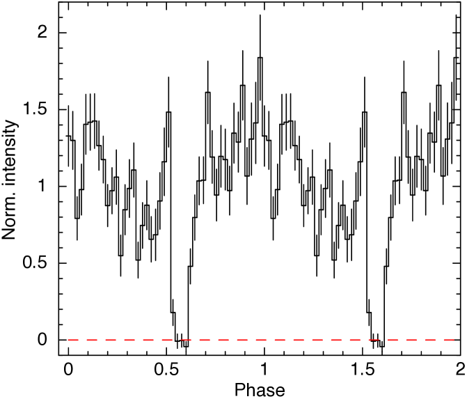
Figure 3: Background-subtracted 0.3–10 keV Swift/XRT light curve folded to the best inferred orbital period of 12 379 s. The total eclipse, lasting about 1.2 ks, is clearly detected and in agreement with those displayed by the XMM–Newton EPIC and OM instruments.

2.5 Spectral analysis

We tested a few simple models for the three XMM–Newton/EPIC (pn + 2 MOSs, excluding the time of the eclipse) and Swift/XRT X-ray spectra of Sw J2014: power law, blackbody and thermal bremsstrahlung, all modified for the interstellar absorption. The spectra were grouped so as to have a minimum of 20 counts for energy channel, and the spectral fits were performed in the 1–10 keV energy band, owing to the very low signal-to-noise of the source data below 1 keV. All these models provide a satisfying fit to the data, but the temperature is totally unconstrained for the bremsstrahlung. For this reason, in Table 2 we summarize the results only for the power law and blackbody fits.

The spectrum was rather hard in all three data sets, with a photon index $\Gamma\sim 0.8$ (or temperature corresponding to $kT\sim 2$ keV for the blackbody fits). The absorbing column inferred from the power-law fits is of $\sim$4–$5\times 10^{22}$ cm^-2, which is much higher than the Galactic value in that direction ($\sim$$1.3\times 10^{21}$ cm^-2). The measured fluxes show a moderate variability ($\sim$30%) from the 2006 and 2013 Swift data to the 2004 XMM–Newton observation. In the XMM–Newton data, which are those with the best counting-statistics, the $\chi^{2}$ values improve with the addition of a Gaussian emission feature to model an excess around 6.5 keV which is probably due to Fe lines (Fig. 4). The equivalent width (EW) of this feature is $\sim$0.25 keV. For the power-law fit, the reduced $\chi^{2}$ changes from $\chi^{2}_{\nu}=1.18$ for 52 degrees of freedom (dof) to 1.03 for 50 dof.

Table 2: XMM–Newton and Swift X-ray spectroscopy. Errors are at a 1$\sigma$ confidence level for a single parameter of interest.

Obs.	Modela	$N_{\rm H}$	$\Gamma$	$kT$	$R_{\mathrm{BB}}$b	$E$	EW	Obs. fluxc	Unabs. fluxc	$\chi^{2}_{\nu}$ (dof)
		($10^{22}$ cm-2)		(keV)	(m)	(keV)	(keV)	($10^{-12}$ erg cm-2 s-1)
Swift/2006	bb		$2.8\pm 0.5$	$1.8^{+0.2}_{-0.1}$	$10\pm 1$	–	–	$0.81\pm 0.05$	$0.98\pm 05$	0.98 (43)
Swift/2006	pl	$5.1^{+0.9}_{-0.8}$	$1.2\pm 0.2$	–	–	–	–	$0.90\pm 0.05$	$1.37^{+0.11}_{-0.09}$	1.14 (43)
Swift/2013	bb		$0.9\pm 0.2$	$2.4\pm 0.2$	$6.9^{+0.7}_{-0.6}$	–	–	$0.98\pm 0.05$	$1.04\pm 0.05$	0.98 (50)
Swift/2013	pl	$2.1\pm 0.4$	$0.5^{+0.2}_{-0.1}$	–	–	–	–	$1.06\pm 0.05$	$1.22\pm 0.05$	1.15 (50)
XMM	bb		$2.6^{+0.6}_{-0.4}$	$2.2\pm 0.2$	$9\pm 1$	–	–	$1.19\pm 0.06$	$1.38\pm 0.06$	1.11 (52)
XMM	bb+gau		$2.6^{+0.6}_{-0.4}$	$2.1^{+0.2}_{-0.1}$	$9\pm 1$	$6.4^{+0.2}_{-0.1}$	$0.22^{+0.10}_{-0.07}$	$1.18\pm 0.06$	$1.37\pm 0.06$	1.00 (50)
XMM	pl	$5.0^{+0.8}_{-0.7}$	$0.9\pm 0.2$	–	–	–	–	$1.24\pm 0.06$	$1.77^{+0.12}_{-0.10}$	1.18 (52)
XMM	pl+gau	$5.0^{+0.8}_{-0.7}$	$1.0\pm 0.2$	–	–	$6.32^{+0.26}_{-0.05}$	$0.25^{+0.11}_{-0.09}$	$1.23\pm 0.06$	$1.78^{+0.12}_{-0.10}$	1.03 (50)

• xspec models: bb=phabs(bbodyrad), pl=phabs(powerlaw), pl+gau=phabs(powerlaw+gaussian).

• Blackbody radius is calculated at infinity and assuming an arbitrary distance to the source of 1 kpc.

• Observed (absorbed) and unabsorbed fluxes, in the 1–10 keV energy range.

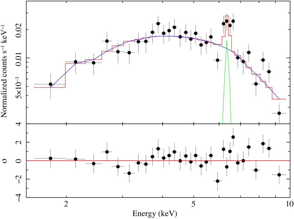
Figure 4: XMM–Newton pn spectrum and best-fitting model [phabs(powerlaw+gaussian), in red]. The blue and green lines show the power-law and Gaussian component, respectively. Bottom panel: the residuals of the fit (in units of standard deviations).

The Swift count rates in the individual observations (see Table 1) show that the variability of Sw J2014 is actually larger than between the combined XRT spectra and XMM–Newton and is of a factor of $\approx$3. In Fig. 5, we show the long-term Swift XRT light curve, together with the simultaneous UVOT near-UV fluxes (when available). The X-ray and UV luminosities are roughly correlated, again suggesting the emissions in the different bands are from the same body. The measured UVOT magnitudes (in the Vega photometric system, see Poole et al. 2008 for more details and Breeveld et al. 2010, 2011 for the most updated zero-points and count rate-to-flux conversion factors) are between $\sim$18.3 and 19.6 for the $uw1$ filter, 18.3 and 19.9 for the $um2$ filter, and 19.14 and 20.3 for the $uw2$ filter. In the XMM–Newton/OM data the observed $B$ magnitude was $\sim$18.9.

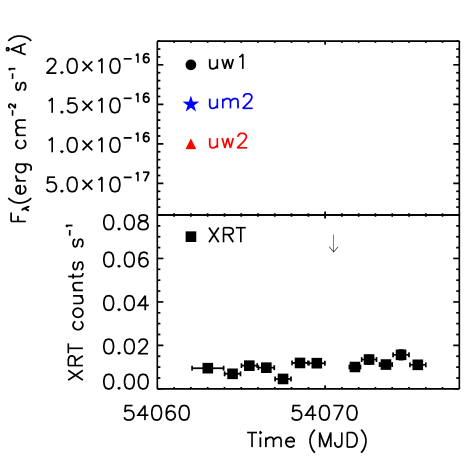
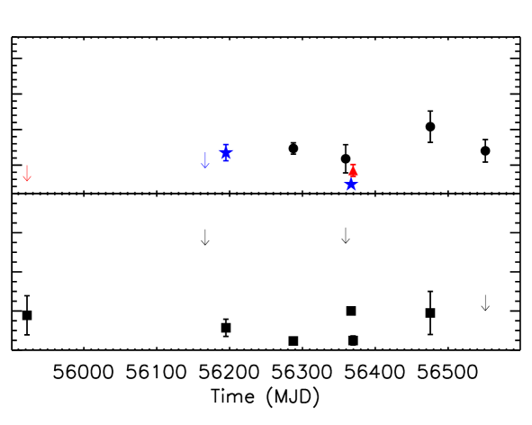
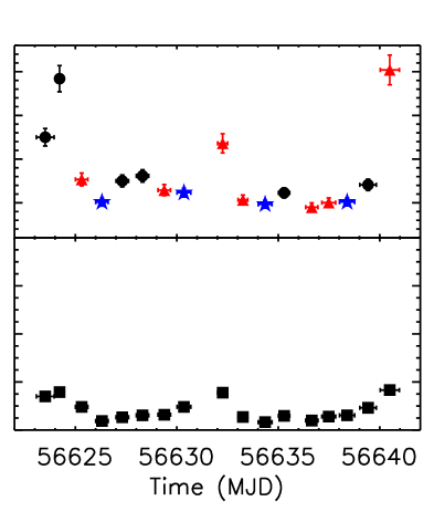
Figure 5: Long-term Swift XRT and UVOT light curve of Sw J2014. Note the time gaps and the different time-scales. The down-arrows indicate upper limits at the 3$\sigma$ confidence level.

3 TNG observations

Sw J2014 optical spectra were obtained on 2011 July 21, August 2 and November 28 (see Table 3) with the 3.58-m TNG equipped with the Device Optimised for the LOw RESolution (DOLORES). The camera is a 2048$\times$2048 E2V 4240 Thinned back-illuminated, deep-depleted CCD with a pixel size of 13.5 $\mu$m. The field of view is 8.6^′$\times$8.6^′ with a 0.252 arcsec pixel^-1 scale. We performed 900 s-long exposures on the target using the low-resolution grism LR-B, which allowed us to obtain a spectral coverage between 3000 and 8400 Å and a dispersion of 2.5 Å pixel^-1.

Table 3: Log of the TNG/DOLORES optical spectroscopy observations.

Spectrum	Date obs. (mid exposure, UT)	Exposure
	(YYYY-MM-DD)	(ks)
1	2011-07-21.00251	0.9
2	2011-08-02.09659	0.9
3	2011-11-28.83850	0.9
4	2011-11-28.84851	0.9
5	2011-11-28.85971	0.9
6	2011-11-28.87042	0.9

Standard data reduction, including bias subtraction and flat-fielding, was performed using different packages in the Image Reduction and Analysis Facility (iraf) package to obtain one-dimensional flux- and wavelength-calibrated spectra. In particular, the spectra were wavelength-calibrated using an Ne+Hg and He reference spectrum. Corrections for atmospheric extinction were also performed. The spectro-photometric standard stars used for the relative flux calibration are: BD +28 4211 (July 21 and November 28 spectra), Feige 110 (August 2 spectrum). The log of spectroscopic observations is reported in Table 3.

The flux-calibrated optical spectra of Sw J2014 display a blue continuum with broad emission lines superposed. We clearly detect H$\alpha$, H$\beta$, H$\gamma$, H$\delta$, Hei ($\lambda\lambda$ 4472, 4713, 4921, 5016–5048, 5876, 6678, 7065 Å), and Heii ($\lambda 4686$). No clear absorption feature is detected. The continuum-normalized average spectrum is shown in Fig. 6.

Figure 6: TNG spectra of Sw J2014. The identified lines as well as the main atmospheric absorption bands are labelled.

The presence of broad (FWHM $\sim 1000$–2000 km s^-1) H and He emission lines favour an origin in an accretion flow on to a compact object, either an NS or a WD. Furthermore, some emission lines show a hint for a double-horned profile, which might be related to the presence of an accretion disc. Several lines show significant intensity variations. The EWs and FWHM for the main detected emission lines obtained by Gaussian fits to the emission profiles are reported in Table 4.

Radial velocities were measured for the four consecutive spectra obtained during the night of 2011 November 28 (spectra 3–6 of Table 3). Relative Doppler shifts were measured with respect to the first spectrum of the series, taken as reference, trough cross-correlation of the main emission lines in the wavelength range 4250–6800 Å. The results are shown in Table 6.

Finally, we note that there might be some variability in the source fluxes observed by TNG. In particular, in the night of 2011 November 28 (Table 3), when four observations were carried out within hours, the fluxes were $6.7\times 10^{-14}$, $7.8\times 10^{-14}$, $8.2\times 10^{-14}$, and $7.6\times 10^{-14}$ erg cm^-2 s^-1 for the four spectra in chronological order (we estimate an uncertainty on the fluxes of 20%). These values are consistent with each other within the uncertainties, but the nominal variability, if true, could be due to the orbital motion, and also effects of the spin rotation cannot be excluded.

Table 4: Results of optical emission lines analysis.

Spectrum	EW	FWHM
	(Å)	(km s-1)
H$\delta$
1	$-3.4\pm 1.4$	$2259\pm 446$
2	$-11.4\pm 2.3$	$1667\pm 204$
3	$-11.3\pm 4.6$	$2049\pm 775$
4	$-15.0\pm 4.0$	$2610\pm 1718$
5	$-13.3\pm 5.7$	$2186\pm 738$
6	$-$	$2932\pm 2303$
H$\gamma$
1	$-5.6\pm 1.4$	$2031\pm 276$
2	$-25.7\pm 2.1$	$1368\pm 110$
3	$-25.0\pm 3.8$	$1347\pm 165$
4	$-16.1\pm 3.0$	$1485\pm 241$
5	$-10.7\pm 3.7$	$1561\pm 214$
6	$-9.8\pm 4.1$	$1326\pm 241$
H$\beta$
1	$-12.9\pm 0.9$	$1852\pm 204$
2	$-57.5\pm 1.2$	$124\pm 74$
3	$-61.5\pm 1.9$	$1179\pm 117$
4	$-45.8\pm 1.2$	$1333\pm 86$
5	$-52.1\pm 1.2$	$1568\pm 117$
6	$-43.8\pm 1.6$	$1580\pm 99$
H$\alpha$
1	$-7.9\pm 2.5$	$950\pm 192$
2	$-119.2\pm 1.5$	$1049\pm 32$
3	$-127.5\pm 2.2$	$905\pm 41$
4	$-120.5\pm 1.8$	$1087\pm 32$
5	$-125.3\pm 1.4$	$1220\pm 32$
6	$-107.5\pm 2.3$	$1295\pm 32$
Hei 4472
1	$-$	$1375\pm 1053$
2	$-5.9\pm 1.3$	$1677\pm 476$
3	$-8.2\pm 2.0$	$1113\pm 394$
4	$-11.9\pm 1.6$	$2012\pm 550$
5	$-8.4\pm 1.9$	$1489\pm 442$
6	$-10.6\pm 2.0$	$1522\pm 1006$

Table 5: continued

Results of optical emission lines analysis. Spectrum EW FWHM (Å) (km s^-1) Hei 5876 1 $-$ $-$ 2 $-21.7\pm 1.7$ $873\pm 97$ 3 $-20.1\pm 2.5$ $959\pm 144$ 4 $-17.6\pm 2.0$ $1082\pm 144$ 5 $-8.0\pm 2.2$ $1296\pm 168$ 6 $-12.1\pm 2.4$ $1322\pm 178$ Hei 6678 1 $-2.0\pm 1.6$ $485\pm 359$ 2 $-10.6\pm 1.1$ $1295\pm 220$ 3 $-5.2\pm 1.3$ $1412\pm 296$ 4 $-8.1\pm 1.1$ $1057\pm 251$ 5 $-6.1\pm 1.0$ $1902\pm 517$ 6 $-7.5\pm 1.3$ $1511\pm 814$ Hei 7065 1 $-3.0\pm 1.4$ $322\pm 106$ 2 $-$ $-$ 3 $-7.7\pm 1.3$ $569\pm 219$ 4 $-5.9\pm 1.2$ $1397\pm 369$ 5 $-3.9\pm 1.0$ $985\pm 318$ 6 $-5.7\pm 1.5$ $2263\pm 598$ Heii 4686 3-6^a $-8.2\pm 0.6$ $1325\pm 211$

• Values obtained from the average of the spectra 3, 4, 5, and 6.

Table 6: Radial velocities of the main spectral emission lines cross-correlating the November 28 spectra in the wavelength range 4250–6800 Å. Spectrum no. 3 was used as reference.

Spectrum	Date obs. (mid exposure)	Radial velocity
	YYYY-MM-DD	km s-1
3	2011-11-28.83850	–
4	2011-11-28.84851	$-12.3\pm 10.8$
5	2011-11-28.85971	$-6.4\pm 7.5$
6	2011-11-28.87042	$96.8\pm 19.4$

4 Loiano observations

Optical photometric data were secured during the night of 2011 September 20 at the Cassini 1.52-m Telescope in Loiano (Italy) using the Bologna Faint Object Spectrograph & Camera (BFOSC). The data set consists of 200 images acquired in the $V$ filter in windowed mode, i.e. selecting a central box of 670$\times$355 pixel, to improve the readout speed. The images have an exposure time of 80 s each and were obtained during a 4.5 h time interval from UT 18:54 to UT 23:31. The sky conditions were clear, although non-photometric, and the average seeing was around $2\aas@@fstack{\prime\prime}5$.

The images were processed using standard procedures and bias and flat-field frames acquired in the same night. All the images were carefully registered and co-added to generate a master frame that was used to obtain a master list of objects. This list was then used as input for the daophot pipeline in the iraf package, and point spread function photometry, as well as aperture correction, were obtained. The magnitudes were then reported to one of them chosen as master (frame #117) because of its good overall quality (good seeing and ellipticity, resulting in a smaller scatter in a plot of instrumental magnitude versus internal photometric error). Information on the target and five comparison stars was then extracted and a light curve was created. Since the night was non-photometric, no photometric standards were available. Moreover, this portion of sky is not included in almost any optical survey. Therefore, we decided to calibrate our $V$ instrumental magnitudes by using the photographic $V$ magnitude in the Guide Star Catalog ver. 2.3 (GSK 2.3; Lasker et al., 2008), which has many stars in our field of view (the same catalogue was also used to improve the astrometry). The calibration is not extremely precise also because we have only one band and thus no colour term correction is possible. We derived a zero-point ${\mathrm{z.p.}_{V}=23.1\pm 0.1}$.

Only one optical source in the BFOSC images is consistent with the XMM–Newton position of Sw J2014, even allowing for a generous error radius of 2 arcsec (see Fig. 7). Best-fitting position (J2000): $\rm RA=20^{h}14^{m}24\aas@@fstack{s}91,~{}Dec.=+15\degr 29^{\prime}30\aas@@fstack{\prime\prime}0$ (J2000, not heliocentric corrected); the uncertainty is dominated by the seeing ($\sim$1^′′). The position of the optical counterpart of Sw J2014 is consistent with those reported in the USNO A2 and B1 catalogues. In particular we identify it with the USNO A2 star U1050-16948097 at $\rm RA=20^{h}14^{m}24\aas@@fstack{s}98,~{}Dec.=+15\degr 29^{\prime}30\aas@@fstack{\prime\prime}6$, reported in the catalogue at $R=18.8$ and $B=18.4$. It is also identified with the older USNO B1 star 1054-0559015 at $\rm RA=20^{h}14^{m}24\aas@@fstack{s}9,~{}Dec.=+15\degr 29^{\prime}30\aas@@fstack{\prime\prime}5$ reported with $B=19.3$, $R=18.7$ and $I=18.5$.

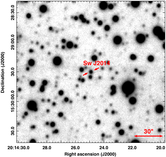
Figure 7: Loiano $B$-band image of the field of Sw J2014 (marked and labelled). The net exposure was 80 s. The image side is 2.5 arcmin wide.

Figure 8 shows the $V$-band Loiano light curve of the Sw J2014’s optical counterpart. There is a clear evidence for an eclipsing event lasting about 35 min. The eclipse can be modelled by a Gaussian centred at MJD 55 825.36254(9) and with $\sigma=414\pm 10$ s ($6.90\pm 0.17$ min). The FWHM duration of the eclipse is $973\pm 22$ s ($16.2\pm 0.4$ min). These values are consistent with the ones obtained from the X-ray eclipse. From the light curve, it is not possible to tell whether a flat bottom is present in the eclipse. A fit with a piecewise linear model to the data constrained the duration of the flat-bottom part – if present – at $<$0.4 ks (at 3$\sigma$), while the inferred ingress and egress lengths are $0.5\pm 0.1$ ks. We searched the light curve for the 491 and 12 379-s modulations, but none could be found, with a 3$\sigma$ upper limit of 0.03 mag on both signals.

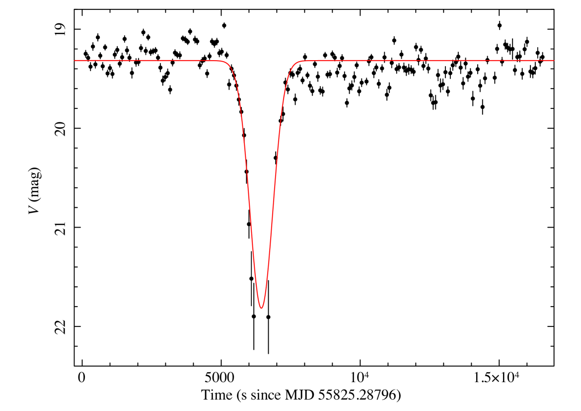
Figure 8: Loiano $V$-band light curve of Sw J2014. The red, solid line indicates the constant-plus-Gaussian model used to infer the time and the duration of the eclipse.

5 Discussion

We have presented X-ray and optical data of the previously unknown X-ray source SwJ2014. Its X-ray position has been determined with XMM–Newton at the J2000 coordinates $\rm RA=20^{h}14^{m}24\aas@@fstack{s}96,~{}Decl.=+15\degr 29^{\prime}29\aas@@fstack{\prime\prime}04$, with an uncertainty of $\sim$$1\aas@@fstack{\prime\prime}5$. This allowed us to identify the optical counterpart of Sw J2014 with the NOMAD source 1054–0592809 ($B\sim 19.3,~{}R\sim 18.9$), at the catalogued position $\rm RA=20^{h}14^{m}24\aas@@fstack{s}899,~{}Decl.=+15\degr 29^{\prime}30\aas@@fstack{\prime\prime}51$. We detected X-ray pulsations at 491 s, which indicate that Sw J2014 harbours a compact star, either a WD or a NS. The pulses are sinusoidal, with a substantial pulsed fraction (40–50%) and there is some hint of a decreasing trend of the pulsed fraction with increasing photon energy. The presence of an additional feature in the X-ray light curves, a permanent eclipse, is a clear signature of an accreting binary with high inclination, $i\geqslant 80\degr$. The X-ray eclipses are total, with a duration of about 20 min, and eclipses are also observed in the optical band, with similar duration. This allowed us to determine an orbital period of 3.44 h for the system. The optical spectrum is dominated by typical accretion features, which indicate the presence of an accretion disc. It is then conceivable that the eclipses in the two bands are related to the eclipse of the compact star and its accretion regions by the donor star, which is undetectable in our optical spectra. The short orbital period would indicate a late type companion of spectral type M4, according tho the orbital period–spectral type relation by Smith & Dhillon (1998).

The stability of the period over a time-span of several years suggests a WD. In fact, due to their larger momentum of inertia, WDs are much harder to spin-up or spin-down than NSs (e.g. Patterson 1994; Bildsten et al. 1997). A magnetic CV of the intermediate polar (IP) type is therefore the favoured interpretation for Sw J2014. Most IPs have spin to orbit period ratio in the range 0.25–0.01 clustering around 0.1 ( Norton, Wynn, & Somerscales 2004; see also Bernardini et al. 2012). The spin to orbit period ratio is 0.04, indicating a rather desynchronized magnetic WD. The orbital period locates this system above the 2–3 h orbital period gap (see e.g. Knigge, Baraffe, & Patterson 2011), where most of the IPs are found. A CV is also favoured by the Balmer and He optical spectral lines. The EW of the H$\beta$ is 45.6 Å (averaged) and that of Heii 4686 is 8.2 Å. The ratio of their EWs are typical of CVs rather than NS systems (van Paradijs & Verbunt, 1984). Moreover, the ratio of the average X-ray to optical fluxes is about 14, which is again more typical for CVs rather than NS binaries, which generally have X-ray fluxes larger by one to two order of magnitudes (Warner, 2003). Also, the orbital X-ray light curve is reminiscent of those observed in IPs (e.g. Parker, Norton, & Mukai 2005), and the possible trend of decreasing pulsed fraction with increasing energy in the spin pulse profile, if real, would be another fairly common feature among IPs (e.g. Rosen, Mason, & Cordova 1988; Norton & Watson 1989). These characteristics observed in IPs are signature of photoelectric absorption, being the former produced by material at the impact region at the disc rim and the latter by dense material in the magnetically channeled accretion flow.

The X-ray spectrum is hard ($\Gamma\sim 1$) and highly absorbed ($N_{\rm H}\sim 5\times 10^{22}$ cm^-2) indicating the presence of dense material close to the compact star. A blackbody fit gives an unacceptable temperature if the X-ray emission arises from a WD. Also the radius derived is unfeasible, since it is too small (few metres) for both WD and NS, even assuming a large distance. An optically thin component is unconstrained therefore preventing direct comparisons with X-ray spectra of IPs, which are characterized by heavily absorbed multi-temperature plasma (e.g. Ishida, Mukai, & Osborne 1994; Beardmore, Osborne, & Hellier 2000) and in many cases by a soft blackbody component with temperatures of tens of eV (e.g. de Martino et al. 2004; Anzolin et al. 2008, 2009). On the other hand, X-ray spectra of quiescent NS low mass, short-period systems are characterized by a soft blackbody component arising from the NS atmosphere but also with lower temperature than that derived. Higher temperatures up to 3 keV are generally detected during X-ray bursts (e.g. Galloway et al. 2008).

Another piece of evidence in favour of a CV classification is the value of the spin period itself. X-ray binaries (XRBs) containing a NS (NS–XRBs) are usually classified based on the spectral type of the donor, for evolutionary reasons: NS–XRBs with late type companions are named low mass X-ray binaries (LMXBs), while NS–XRBs hosting massive early type stars are called high mass X-ray binaries. A third class of (rare) accreting NS–XRBs has been more recently recognized, thanks to the growing number of members (e.g. Corbet et al. 2008). They are the so-called symbiotic (NS) binaries (SyXBs). Although some of them are known since the early times of X-ray astronomy (e.g. GX 1+4; Lewin, Ricker, & McClintock 1971), and were at first classified as LMXBs, SyXBs display completely different properties (see e.g. Masetti et al. 2006; Corbet et al. 2008), like slow NS pulsations, M-type giant companions and very wide orbits (for example, GX 1+4, has P_spin=114 s and P_orb=1 160.8 d). On the contrary, LMXBs where pulsations have been detected display NS spin periods typically in the millisecond range, reaching, at maximum, a spin period of $\sim$7.7 s in the LMXB 4U 1626–67 (Liu, van Paradijs, & van den Heuvel 2007; see also figs. 1 and 13 in Enoto et al. 2014). Given the typical properties characterizing LXMBs and SyXBs, the two periodicities we discovered in Sw J2014 (spin period of 491 s and orbital period of 3.44 h) make an association with an XRB containing a NS as compact object very unlikely. Indeed, this would place the source in a completely empty portion of the so-called Corbet diagram of the NS spin period versus the orbital period of the system (see an updated version of this diagram in fig. 13 of Enoto et al. 2014). In conclusions, while the X-ray spectra cannot constrain the type of source, all the other pieces of evidence indicate that Sw J2014 hosts a WD, and is thus a magnetic CV of the IP type.

In the hypothesis that Sw J2014 consists of a WD accreting from a Roche lobe-filling, low-mass, main-sequence star, with standard considerations (e.g. Paczyński 1971), making the approximations of a circular orbit and $\sin i\simeq 1$, and assuming standard stellar mass–radius relations (e.g. Smith & Dhillon 1998; Knigge 2006), we can estimate the donor mass and radius as $M_{\bigstar}\approx 0.3~{}\mathrm{M_{\sun}}$ and $R_{\bigstar}\approx 0.4~{}\mathrm{R_{\sun}}$. If for the WD mass we take 0.8 $\mathrm{M_{\sun}}$, which is a reasonable value in CVs (Zorotovic, Schreiber, & Gänsicke, 2011), we get from Kepler’s third law an estimate for the binary separation of $a\approx 1.2~{}\mathrm{R_{\sun}}$. Considering the $\sim$0.2 ks ingress/egress duration, the linear size of the X-ray-emitting region should be of the order of $\approx$$0.05~{}\mathrm{R_{\sun}}$ (for $i=80\degr$; see equation 1 of Nucita et al. 2009; see also Wheatley & West 2003). This is $\sim$5 times the radius that can be expected for a 0.8 $\mathrm{M_{\sun}}$ WD, but considered the large uncertainties the value is consistent with the X-rays being emitted from the WD or close to it, and also with estimates of the inner radius of the truncated disc of a CV (e.g. Mhlahlo et al. 2007; Dobrotka, Mineshige, & Ness 2014). Future multiband observations should be able to provide tight constraints on the system parameters.
We finally notice that, assuming $1.8\times 10^{-12}$ erg cm^-2 s^-1 for the unabsorbed X-ray flux of Sw J2014 (Table 2), the X-ray luminosity of the source is $L_{\mathrm{X}}\simeq 2\times 10^{32}d^{2}_{1}$ erg s^-1, where $d_{1}$ is the distance in units of 1 kpc. For a few kpc, this is consistent with typical values for IPs ($10^{32}$–$10^{34}$ erg s^-1; e.g. Sazonov et al. 2006).

6 Summary

In this paper, we reported on the SATS @ BAR discovery of the new X-ray pulsator Sw J2014. The periodicity of 491 s indicates that Sw J2014 harbours a compact star. Follow-up observations to investigate the nature of the source were done both with space-borne (Swift and XMM–Newton) and ground-based (TNG and Loiano Telescope) facilities.
The XMM–Newton EPIC and OM light curves both show a sudden drop of the flux followed by a quick recovery, similar to the deep/total eclipses in NS–LMXBs or CVs with high inclination. The time lag between the X-ray and the optical eclipses is $\Delta t_{\rm eclipses}\simeq 12.4$ ks. Unfortunately, the EPIC and OM data are not simultaneous, but the Swift monitoring campaign provided us evidence indicating that $\Delta t_{\rm eclipses}$ is the orbital period of the system, and thus that the X-ray and optical eclipses are simultaneous (and that the $491$-s periodicity is the rotation period of the compact object). The X-ray spectra are quite hard (with photon index $\Gamma{}\sim{}0.8$). Optical spectra allowed us to measure several emission lines, which are consistent with an accretion disc. Photometry led to the identification of the optical counterpart (the NOMAD star 1054–0592809).
The nature of the compact star (i.e. whether it is a NS or a WD) cannot be definitely assessed by our data but, in the case of a NS, Sw J2014 would lie in a completely empty portion of the Corbet diagram for spin versus orbital period. On the other hand, several pieces of information (including the long spin period and its stability over a time-span of several years, the EWs and the ratio of the H$\beta$ and Heii 4686) point towards a WD. We are thus confident that Sw J2014 is a magnetic CV of the IP type. In particular, Sw J2014 is a potential addition to the very small number of known deeply-eclipsing IPs (Walker 1956; Hellier 1997; Hellier, Mukai, & Beardmore 1997; Woudt & Warner 2003; Warner & Woudt 2009; Aungwerojwit et al. 2012). These systems are very important since they allow accurate measurements of the system parameters and the possibility to study the geometry of the X-ray emitting regions (see e.g., Hellier 2014).

References

- Allan et al. (1998) Allan A., Hellier C., Beardmore A., 1998, MNRAS, 295, 167
- Anzolin et al. (2008) Anzolin G., de Martino D., Bonnet-Bidaud J.-M., Mouchet M., Gänsicke B. T., Matt G., Mukai K., 2008, A&A, 489, 1243
- Anzolin et al. (2009) Anzolin G., de Martino D., Falanga M., Mukai K., Bonnet-Bidaud J.-M., Mouchet M., Terada Y., Ishida M., 2009, A&A, 501, 1047
- Aungwerojwit et al. (2012) Aungwerojwit A., Gänsicke B. T., Wheatley P. J., Pyrzas S., Staels B., Krajci T., Rodríguez-Gil P., 2012, ApJ, 758, 79
- Beardmore et al. (2000) Beardmore A. P., Osborne J. P., Hellier C., 2000, MNRAS, 315, 307
- Bernardini et al. (2012) Bernardini F., de Martino D., Falanga M., Mukai K., Matt G., Bonnet-Bidaud J.-M., Masetti N., Mouchet M., 2012, A&A, 542, A22
- Bildsten et al. (1997) Bildsten L. et al., 1997, ApJS, 113, 367
- Breeveld et al. (2010) Breeveld A. A. et al., 2010, MNRAS, 406, 1687
- Breeveld et al. (2011) Breeveld A. A., Landsman W., Holland S. T., Roming P., Kuin N. P. M., Page M. J., 2011, in AIP Conference Proceedings, Vol. 1358, Gamma Ray Bursts 2010., J. E. McEnery, J. L. Racusin, & N. Gehrels, ed., AIP, Melville, pp. 373–376
- Burrows et al. (2005) Burrows D. N. et al., 2005, Space Science Reviews, 120, 165
- Corbet et al. (2008) Corbet R. H. D., Sokoloski J. L., Mukai K., Markwardt C. B., Tueller J., 2008, ApJ, 675, 1424
- de Martino et al. (2004) de Martino D., Matt G., Belloni T., Haberl F., Mukai K., 2004, A&A, 415, 1009
- de Martino et al. (2005) de Martino D. et al., 2005, A&A, 437, 935
- Dobrotka et al. (2014) Dobrotka A., Mineshige S., Ness J.-U., 2014, MNRAS, 438, 1714
- Enoto et al. (2014) Enoto T. et al., 2014, ApJ, 786, 127
- Esposito et al. (2013a) Esposito P., Israel G. L., Sidoli L., Mapelli M., Zampieri L., Motta S. E., 2013a, MNRAS, 436, 3380
- Esposito et al. (2013b) Esposito P., Israel G. L., Sidoli L., Mason E., Rodríguez Castillo G. A., Halpern J. P., Moretti A., Götz D., 2013b, MNRAS, 433, 2028
- Esposito et al. (2013c) Esposito P., Israel G. L., Sidoli L., Rodríguez Castillo G. A., Masetti N., D’Avanzo P., Campana S., 2013c, MNRAS, 433, 3464
- Esposito et al. (2014) Esposito P., Israel G. L., Sidoli L., Tiengo A., Campana S., Moretti A., 2014, MNRAS, 441, 1126
- Frank et al. (2002) Frank J., King A., Raine D. J., 2002, Accretion Power in Astrophysics: Third Edition. Cambridge: Cambridge University Press
- Galloway et al. (2008) Galloway D. K., Muno M. P., Hartman J. M., Psaltis D., Chakrabarty D., 2008, ApJS, 179, 360
- Gehrels et al. (2004) Gehrels N. et al., 2004, ApJ, 611, 1005
- Götz et al. (2013) Götz D., Covino S., Fernández-Soto A., Laurent P., Bošnjak Ž., 2013, MNRAS, 431, 3550
- Hellier (1997) Hellier C., 1997, MNRAS, 291, 71
- Hellier (2014) Hellier C., 2014, in European Physical Journal Web of Conferences, Vol. 64, European Physical Journal Web of Conferences, p. 7001
- Hellier et al. (1998) Hellier C., Beardmore A. P., Buckley D. A. H., 1998, MNRAS, 299, 851
- Hellier et al. (1997) Hellier C., Mukai K., Beardmore A. P., 1997, MNRAS, 292, 397
- Ishida et al. (1994) Ishida M., Mukai K., Osborne J. P., 1994, PASJ, 46, L81
- Jansen et al. (2001) Jansen F. et al., 2001, A&A, 365, L1
- Kalberla et al. (2005) Kalberla P. M. W., Burton W. B., Hartmann D., Arnal E. M., Bajaja E., Morras R., Pöppel W. G. L., 2005, A&A, 440, 775
- Kirsch et al. (2004) Kirsch M. G. F. et al., 2004, in UV and Gamma-Ray Space Telescope Systems. Proceedings of the SPIE. SPIE, Bellingham WA, Hasinger G., Turner M. J. L., eds., Vol. 5488, p. 103
- Knigge (2006) Knigge C., 2006, MNRAS, 373, 484
- Knigge et al. (2011) Knigge C., Baraffe I., Patterson J., 2011, ApJS, 194, 28
- Lasker et al. (2008) Lasker B. M. et al., 2008, AJ, 136, 735
- Lewin et al. (1971) Lewin W. H. G., Ricker G. R., McClintock J. E., 1971, ApJ, 169, L17
- Liu et al. (2007) Liu Q. Z., van Paradijs J., van den Heuvel E. P. J., 2007, A&A, 469, 807
- Masetti et al. (2006) Masetti N., Orlandini M., Palazzi E., Amati L., Frontera F., 2006, A&A, 453, 295
- Mason et al. (2001) Mason K. O. et al., 2001, A&A, 365, L36
- Mhlahlo et al. (2007) Mhlahlo N., Buckley D. A. H., Dhillon V. S., Potter S. B., Warner B., Woudt P. A., 2007, MNRAS, 378, 211
- Nichelli et al. (2009) Nichelli E., Israel G. L., Moretti A., Campana S., Bernabei S., Mason E., Götz D., Stella L., 2009, Astron. Tel., 2354
- Norton & Watson (1989) Norton A. J., Watson M. G., 1989, MNRAS, 237, 853
- Norton et al. (2004) Norton A. J., Wynn G. A., Somerscales R. V., 2004, ApJ, 614, 349
- Nucita et al. (2009) Nucita A. A., Maiolo B. M. T., Carpano S., Belanger G., Coia D., Guainazzi M., de Paolis F., Ingrosso G., 2009, A&A, 504, 973
- Paczyński (1971) Paczyński B., 1971, ARA&A, 9, 183
- Parker et al. (2005) Parker T. L., Norton A. J., Mukai K., 2005, A&A, 439, 213
- Patterson (1994) Patterson J., 1994, PASP, 106, 209
- Poole et al. (2008) Poole T. S. et al., 2008, MNRAS, 383, 627
- Roming et al. (2005) Roming P. W. A. et al., 2005, Space Science Reviews, 120, 95
- Rosen et al. (1988) Rosen S. R., Mason K. O., Cordova F. A., 1988, MNRAS, 231, 549
- Sazonov et al. (2006) Sazonov S., Revnivtsev M., Gilfanov M., Churazov E., Sunyaev R., 2006, A&A, 450, 117
- Smith & Dhillon (1998) Smith D. A., Dhillon V. S., 1998, MNRAS, 301, 767
- Strüder et al. (2001) Strüder L. et al., 2001, A&A, 365, L18
- Turner et al. (2001) Turner M. J. L. et al., 2001, A&A, 365, L27
- van Paradijs & Verbunt (1984) van Paradijs J., Verbunt F., 1984, in AIP Conference Series, Vol. 115, High Energy Transients in Astrophysics, Woosley S. E., ed., AIP, Melville, pp. 49–62
- Vaughan et al. (1994) Vaughan B. A. et al., 1994, ApJ, 435, 362
- Walker (1956) Walker M. F., 1956, ApJ, 123, 68
- Warner (2003) Warner B., 2003, Cataclysmic Variable Stars. Cambridge, UK: Cambridge University Press
- Warner & Woudt (2009) Warner B., Woudt P. A., 2009, MNRAS, 397, 979
- Weisskopf et al. (2002) Weisskopf M. C., Brinkman B., Canizares C., Garmire G., Murray S., Van Speybroeck L. P., 2002, PASP, 114, 1
- Wheatley & West (2003) Wheatley P. J., West R. G., 2003, MNRAS, 345, 1009
- Woudt & Warner (2003) Woudt P. A., Warner B., 2003, MNRAS, 340, 1011
- Zacharias et al. (2005) Zacharias N., Monet D. G., Levine S. E., Urban S. E., Gaume R., Wycoff G. L., 2005, VizieR Online Data Catalog, 1297, 0
- Zorotovic et al. (2011) Zorotovic M., Schreiber M. R., Gänsicke B. T., 2011, A&A, 536, A42