Long-lived resonances at mirrors.

Abstract

Motivated by realistic scattering processes of composite systems, we study the dynamics of a two-particle bound system which is scattered at a mirror. We consider two different scenarios: In the first case we assume that only one particle interacts directly with the mirror whereas in the second case both particles are scattered. The coherence between the transmitted and the reflected wave-packet is reduced when the internal degree of freedom (the relative coordinate) of the bound system becomes excited. Depending on the particular system-mirror interaction, long-lived resonances can occur.

I Introduction.

The superposition principle is of prime importance in quantum mechanics and has been demonstrated for neutrons SBRKZ83 , in superconductors RHL95 ; CCDEM88 ; SPRR97 ; NPT99 , in nanomagnets FSTZ96 ; B99 ; W97 , with trapped ions MMKW96 , with photons in cavities B96 and for large molecules ANVKKZZ99 . Nevertheless, interferences of macroscopic objects are not yet accessible RCNSC11 . Macroscopic Schrödinger Cat states are of particular interest in the context of the quantum-to-classical transition S07 ; Z03 ; C13 , tests of collapse models BG03 ; GPR90 ; R11 ; BLSSU14 and the search for gravitational decoherence KHKRSJA12 ; B12 ; AL13 ; BGL08 ; SQ15 ; GU14 . A major difficulty is the strong suppression of coherences since macroscopic systems cannot be isolated completely from their environment and the emission and absorption of blackbody radiation washes out the interference pattern KHKRSJA12 .

The preparation of a spatial (macroscopic) superposition requires that the wavefunction of the composite object is split into two (or more) components. This can be done, for example, with an apparatus which acts as a partially silvered mirror, separating the incoming wave-packet into a reflected and a transmitted part. In the following we will show that long-lived resonances can occur due to the presence internal degrees of freedom of the composite object. Furthermore, the wavepacket components can decohere partially when internal degrees of freedom are excited during the scattering process. These effects are also present when the system is perfectly isolated from the environment.

During a scattering process of a composite object, it is likely that not all individual constituents interact directly with the mirror. For example, Rutherford-scattering affects only the protons of $\alpha$-particles directly whereas the neutrons do not feel the Coulomb potential of the heavy nuclei. Since the protons and neutrons are bound to each other by nuclear forces, the neutrons follow the trajectory of the protons. The situation that only a part of the composite object interacts with a scattering center is rather generic, the atom-light interaction being another example: Only the dipole moment of the electron is affected by the electromagnetic field whereas the nucleus is not sensitive to the wavelength of the photons.

A simple model Hamiltonian, which resembles the interaction of an single (center-of-mass) degree of freedom with a mirror, is

$$\hat{H}=\frac{\hat{p}^{2}}{2}+\hat{V}(\hat{x})\,,$$ (1)

where we assume that the potential has the form $\hat{V}(\hat{x})=V_{\mathrm{m}}\delta(\hat{x})$. An incoming plane wave with momentum $k$ will be partially transmitted and reflected, i.e.

$$\psi_{k}(x)=\begin{cases}e^{ikx}+re^{-ikx}&\text{for }x<0\\ te^{ikx}&\text{for }x>0\,,\end{cases}$$ (2)

where the amplitudes for transmission and reflection are determined by

$$t=\frac{k}{k+iV_{\mathrm{m}}}\quad\text{and}\quad r=-\frac{iV_{\mathrm{m}}}{k+iV_{\mathrm{m}}}\,.$$ (3)

Choosing $k=V_{\mathrm{m}}$ we have $|t|^{2}=|r|^{2}=1/2$ which mimics a half-silvered mirror. The system exhibits a resonance for $ik_{\mathrm{res}}=V_{\mathrm{m}}>0$ and a bound state for $V_{\mathrm{m}}<0$. Since we have $\mathrm{Re}(k_{\mathrm{res}})=0$, the dynamics of a wavepacket which is centered around a finite momentum value will not be affected by the resonance. In the following we will see how the situation changes when the dynamics of internal degrees of freedom is taken into account.

II The model.

Consider two particles with unit mass and coordinates $x_{1}$ and $x_{2}$. Both particles are tied to each other by a binding potential $\hat{V}_{\mathrm{b}}$ which depends only on the difference of the particle positions, $x_{\mathrm{rel}}=x_{1}-x_{2}$. In general, we allow both particles to interact with a mirror and introduce the scattering potentials $V_{\mathrm{m}}^{1/2}\delta(\hat{x}_{1/2})$. The Hamiltonian which describes the scattering of this bound system is given by

$$\hat{H}=\frac{\hat{p}_{1}^{2}}{2}+\frac{\hat{p}_{2}^{2}}{2}+V^{1}_{\mathrm{m}}\delta(\hat{x}_{1})+V^{2}_{\mathrm{m}}\delta(\hat{x}_{2})+\hat{V}_{\mathrm{b}}(\hat{x}_{1}-\hat{x}_{2})\,,$$ (4)

Figure 1: When the particles are bound to each other by a hard wall potential, the system corresponds to a two-dimensional waveguide. The scattering potential $V_{\mathrm{m}}^{1}\delta(\hat{x}_{1})$ is nonzero along the dotted line whereas $V_{\mathrm{m}}^{2}\delta(\hat{x}_{2})$ is nonzero along the dashed line.

where $\hat{p}_{1,2}$ are the momentum operators of the individual particles.

It is useful to formulate the problem in terms of the center-of-mass coordinate $\hat{x}_{\mathrm{cm}}=\hat{x}_{1}+\hat{x}_{2}$ and the relative coordinate $\hat{x}_{\mathrm{rel}}=\hat{x}_{1}-\hat{x}_{2}$. An arbitrary wave-packet is of the form

$$\Psi=\sum_{n}f_{n}(x_{\mathrm{cm}},t)\phi_{n}(x_{\mathrm{rel}})\,,$$ (5)

where the $f_{n}$ are time-dependent functions which only depend center-of-mass coordinate and the $\phi_{n}$ fulfill eigenvalue equation

$$-\frac{d^{2}\phi_{n}}{dx_{\mathrm{rel}}^{2}}+V_{\mathrm{b}}(x_{\mathrm{rel}})\phi_{n}=\epsilon_{n}\phi_{n}\,.$$ (6)

The choice of the binding potential determines how far the particles can separate from each other. When we choose a hard wall potential, the system is related to a two-dimensional waveguide, see Fig. 1.

Inserting the ansatz (5) into the time-dependent Schrödinger equation, multiplying with $\phi_{m}(x_{\mathrm{rel}})$ and integrating over $x_{\mathrm{rel}}$ leads to a set of coupled equations,

$$i\partial_{t}f_{n}=-\frac{d^{2}f_{n}}{dx_{\mathrm{cm}}^{2}}+\epsilon_{n}f_{n}+\sum_{m}V_{nm}(x_{\mathrm{cm}})f_{m}\,.$$ (7)

$V_{nm}$ is the effective potential which couples the functions $f_{n}$. It can be expressed in terms of the eigenfunctions $\phi_{n}$ of the binding potential,

$$V_{nm}(x_{\mathrm{cm}})= 2V^{1}_{\mathrm{m}}\phi_{n}(-x_{\mathrm{cm}})\phi_{m}(-x_{\mathrm{cm}})$$

$$+2V^{2}_{\mathrm{m}}\phi_{n}(x_{\mathrm{cm}})\phi_{m}(x_{\mathrm{cm}})\,.$$ (8)

We assume that the wave-packet is initially of the form

$$\Psi_{\mathrm{in}}=\left(\frac{2}{\pi\sigma^{2}}\right)^{1/4}\exp\left(iPx_{\mathrm{cm}}-\frac{(x_{\mathrm{cm},0}-x_{\mathrm{cm}})^{2}}{\sigma^{2}}\right)\phi_{0}(x_{\mathrm{rel}})\,,$$ (9)

where the initial momentum of the center-of-mass coordinate is denoted with $P$ and the spread of the wave packet with $\sigma$. The wave-packet is initially centered to the left of the mirror, $x_{\mathrm{cm},0}\rightarrow-\infty$, and follows a free evolution before it hits the mirror. The “internal” degree of freedom is assumed to be in the ground state $\phi_{0}(x_{\mathrm{rel}})$.

III Harmonic coupling.

A simple binding potential is the harmonic coupling $\hat{V}_{\mathrm{b}}=\Omega^{2}\hat{x}_{\mathrm{rel}}^{2}$ with stiffness $\Omega$. From the eigenvalue equation (6) we find that the energy levels of the internal degree of freedom are $\epsilon_{n}=2\Omega(n+1/2)$. The effective coupling potential $V_{nm}$ is determined by the eigenfunctions of the harmonic oscillator, $\phi_{n}=((\Omega/\pi)^{1/4}/\sqrt{2^{n}n!})H_{n}(\sqrt{\Omega}x_{\mathrm{rel}})\exp(-\Omega x_{\mathrm{rel}}^{2}/2)$.

III.1 Asymmetric scattering, $V^{1}_{\mathrm{m}}=0,V^{2}_{\mathrm{m}}>0$

First, we discuss the situation when only one particle interacts directly mirror whereas particle 2 is only affected indirectly by the mirror via the binding potential. This corresponds to the choice $V_{\mathrm{m}}^{1}=0$ and $V_{\mathrm{m}}^{2}>0$ in our model. In oder to mimic a half-silvered mirror, we choose the parameter $V_{\mathrm{m}}^{1}$ and the initial momentum $P$ such that half of the wave-packet is transmitted and half of it is reflected, In Fig. 2 we show the reduced density matrix $\rho_{\mathrm{cm}}~{}=~{}\int_{-\infty}^{\infty}dx_{\mathrm{rel}}\Psi^{*}(x_{\mathrm{cm}},x_{\mathrm{rel}})\Psi(x^{\prime}_{\mathrm{cm}},x_{\mathrm{rel}})$ and the square of the modulus of the wavefunction at different times. The wavepacket is localized before the scattering process, see Fig. 2 (a). Then, according to the sketch in Fig. 1, the scattering occurs at the line $x_{2}=0$ which can be seen in Fig. 2 (b). After the scattering process, the reflected and transmitted parts of the wavefunction separate from the mirror, see Fig. 2 (c).

The scattering process is not adiabatic and higher modes $\phi_{n}$ ($n>0$) become populated. The initial product state (9) evolves to a general superposition (5). In Fig. 3 (a) and Fig. 3 (b) we depict the time-evolution of $p_{n,\mathrm{L}}=\int_{-\infty}^{0}|f_{n}|^{2}dx_{\mathrm{cm}}$ and $p_{n,\mathrm{R}}=\int^{\infty}_{0}|f_{n}|^{2}dx_{\mathrm{cm}}$ which are the probabilities to find the internal degree of freedom in the state $\phi_{n}$ if the state is measured to the left or to the right from the mirror. Since half of the wavepacket is transmitted and half of it is reflected, we have $\sum_{n}p_{n,\mathrm{L}}=\sum_{n}p_{n,\mathrm{R}}=0.5$ after the scattering.

The composite system is in a pure state which allows us to characterize the excitation of the wave-packet by the entanglement-entropy, $S=-\mathrm{tr}(\hat{\rho}_{\mathrm{cm}}\ln\hat{\rho}_{\mathrm{cm}})$. The entropy changes only during the scattering process since the free time-evolution does not excite the internal degree of freedom, see Fig. 4 (a),

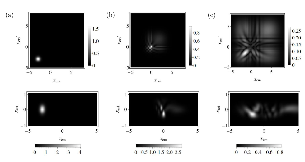
Figure 2: Dynamics of the scattering process. Top: Absolute value of the reduced density matrix $\rho_{\mathrm{cm}}$. Bottom: Absolute value of the wavefunction. (a) Initial configuration of the wavepacket. (b) The scattering process occurs at the line $x_{2}=0$. (c) The reflected part and the transmitted part of the wavefunction are separated from the mirror again.

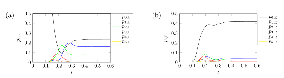
Figure 3: As explained in the text, the internal degree of freedom is more excited in the reflected part (a) than in the transmitted part (b). In order to achieve that after the scattering process half of the wavepacket is transmitted and half of it is reflected, we choose $P=10$, $V^{\mathrm{2}}_{\mathrm{m}}=11$, $\sigma=1/2$ and $\Omega=10$.

Furthermore, the energy of the center-of-mass coordinate and the energy of the internal degree of freedom is different for the reflected and transmitted part of the wave-packet, see Fig. 4 (b). The internal degree is more excited when the bound system is reflected: One particle is reflected by the mirror, the second one passed through and is pulled back through the mirror due to the binding potential $V_{\mathrm{b}}$. This leads to an increased excitation compared to the transmission where both particles go through the mirror without the internal dynamics being involved. This explains why the $p_{i>0,\mathrm{L}}$ (Fig. 3 (a)) are larger than the $p_{i>0,\mathrm{R}}$ (Fig. 3 (b)) for $t\rightarrow\infty$. The reflected and transmitted parts of the center of mass motion become disentangled.

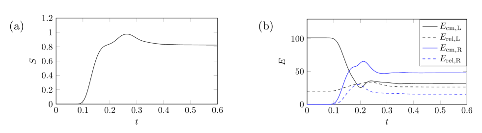
Figure 4: (a) Time-evolution of the entanglement-entropy for asymmetric scattering. (b) Time-evolution of the center-of-mass energy $E_{\mathrm{cm}}=\langle\hat{p}_{\mathrm{cm}}^{2}\rangle$ and the internal energy $E_{\mathrm{rel}}=\langle\hat{p}_{\mathrm{rel}}^{2}+\hat{V}_{\mathrm{b}}\rangle$ of the wave-packet to the left (L) and to the right (R) of the mirror.

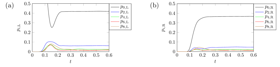
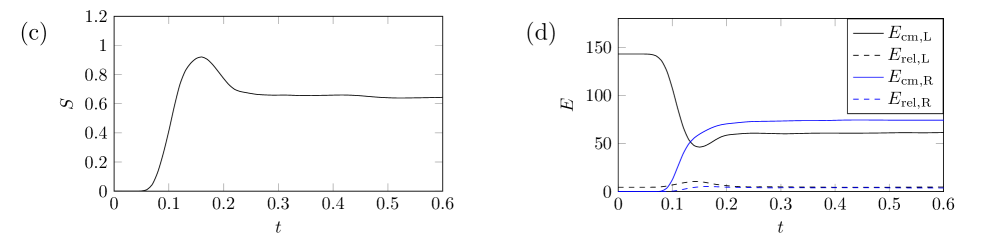
Figure 5: Symmetric scattering of the two-particle bound state. (a) and (b) Time-evolution of the occupation probabilities for the modes of the internal degree of freedom to the left (L) and to the right (R) of the mirror. Due to the symmetry of the scattering potential, the antisymmetric modes are not occupied. In order to achieve that after the scattering process half of the wavepacket is transmitted and half of it is reflected, we choose $P=12$, $V^{\mathrm{1/2}}_{\mathrm{m}}=15$, $\sigma=1/2$ and $\Omega=5$. Time-evolution of the entanglement-entropy (c), the center-of-mass energy and internal energy (d).

III.2 Symmetric scattering, $V^{1}_{\mathrm{m}}=V^{2}_{\mathrm{m}}>0$

In the following we discuss the case when both particles interact directly with the mirror with the same strength, i.e. $V^{1}_{\mathrm{m}}=V^{2}_{\mathrm{m}}>0$. Again, we choose the initial momentum and the value of $V^{1,2}_{\mathrm{m}}$ such that half of the wave-packet is transmitted and half of it is reflected. The scattering potential does not mix the symmetric modes $\phi_{n}$, ($n=0,2,4,...$) with the antisymmetric modes $\phi_{n}$, ($n=1,3,5,...$). Therefore antisymmetric modes do not become excited when the system is initially in the ground state, see Fig. 5. This in turn implies that the energy gap between ground state and first accessible excited state is $\epsilon_{2}-\epsilon_{0}=4\Omega$ rather than $\epsilon_{1}-\epsilon_{0}=2\Omega$. As a consequence, the increase of entanglement-entropy is smaller for the symmetric scattering than it is for the asymmetric scattering, compare Fig. 4 (a) and Fig. 5 (c). Furthermore, the energy transfer from the center-of-mass motion to the relative motion is smaller, compare Fig. 4 (b) and Fig. 5 (d).

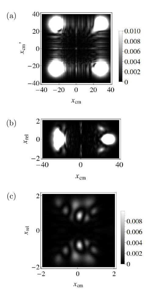
Figure 6: Symmetric scattering of the bound state. (a) Reduced density matrix $\hat{\rho}_{\mathrm{cm}}$ after the scattering. A part of the wavefunction is trapped at the mirror. (b) Wavefunction after the scattering process. (c) The wavefunction is trapped in the triangles which are defined by the lines $x_{1}=0$ and $x_{2}=0$.

An interesting feature of the symmetric scattering is that it takes a rather long time before the occupation probabilities become temporal constants. This is due to the occurence of long-lived resonances. Intuitively, this can be understood from the sketch in Fig. 1: When particle 1 is reflected at $x_{1}=0$, it pulls back particle 2, then particle 2 is reflected at $x_{2}=0$ and particle 1 is pulled back. This can happen several times until the wave-packet finally separates from the mirror. As a result, a part of the wave-function is trapped in the “triangles” for a finite time. Although most of the wave-function has separated from the mirror after the scattering, there is a non-vanishing probability to find the particles at the mirror. The interference pattern of $\hat{\rho}_{\mathrm{cm}}$ after the scattering process is depicted in Fig. 6 (a) whereas the wave-function is shown in Fig. 6 (b). In Fig. 6 (c) one can see how the wave-function is trapped in the triangles.

IV Resonances.

In general, resonances can be characterized as eigenvalues of the Hamiltonian which is subject to non-hermitian boundary conditions. A simple example was given in the introduction: The scattering of a particle at a delta-function potential with positive prefactor $V_{\mathrm{m}}$ exhibits a resonance for the wavenumber $k_{\mathrm{res}}=-iV_{\mathrm{m}}$. The corresponding wave-function is not in the Hermitian sector of the domain of the physical Hamiltonian and grows exponentially for large $|x|$, $\psi\sim e^{V_{\mathrm{m}}|x|}$. In the following we use the complex scaling method to determine the position of the resonances M11 ; M98 ; M78 ; S78 ; RS78 : The core of this method is a transformation of the Hamiltonian such that the resonant eigenfunctions become square integrable. For the problem at hand, this can be achieved by transforming the the center-of-mass coordinate according to $x_{\mathrm{cm}}\rightarrow e^{i\theta}x_{\mathrm{cm}}$. When the angle $\theta$ is large enough, the eigenfunction of a particular resonance decreases exponentially for $|x_{\mathrm{cm}}|\rightarrow\pm\infty$. Thus, the complex energy $E_{\mathrm{res}}$ can be determined from the eigenvalue problem for the transformed Hamiltonian. The value of $E_{\mathrm{res}}$ is locally independent on $\theta$ and appears as isolated point in the spectrum, see Appendix. The life-time $\tau$ of a resonance is determined by the imaginary part of the resonant energy via $\tau=-1/(2\mathrm{Im}E_{\mathrm{res}})$. Thus, the closer the resonant energy is to the real axis, the longer is the decay time.

For asymmetric scattering, we find that the resonances are far away from the real axis, see Fig. 7 (a). However, when both particles interact with the mirror, i.e. $V_{\mathrm{m}}^{1}=V_{\mathrm{m}}^{2}>0$, the resonances can be long-lived, see Fig. 7 (b). The effect on the dynamics becomes apparent from the amplitude of the wavefunction at the mirror: For asymmetric scattering, the amplitude at the mirror vanishes immediately (Fig. 2) whereas the decrease of the amplitude during symmetric scattering is much slower (Fig. 6). In Fig. 8 (a), we show the amplitude for symmetric scattering at various times. Even when the parameters of the model are choosen such that most of the bound system is reflected (corresponding to a totally reflecting mirror), a part of the wave-function is trapped temporarily at the repulsive scattering potential, see Fig. 8 (b).

Figure 7: Spectrum of the Hamiltonian after analytical continuation. The lines denote the continuous part of the spectrum and the blue dots are the resonances. (a) Asymmetric scattering: The parameters are $\Omega=~{}5$, $V_{\mathrm{m}}^{1}=0$, $V_{\mathrm{m}}^{2}=30$ and $\theta=0.35$. The resonances are short-lived when only particle interact directly with the mirror. (b) Symmetric scattering: The parameters are $\Omega=5$, $V_{\mathrm{m}}^{1}=V_{\mathrm{m}}^{2}=30$ and $\theta=0.1$. The resonances can be long-lived when both particles interact directly with the mirror. Note that the inverse life-times $\mathrm{Im}(E)$ for asymmetric scattering (a) and for symmetric scattering (b) differ by a factor of 100 for the same choice of parameters. The resonance which is closest to the real axis has an inverse lifetime of $|\mathrm{Im}(E_{\mathrm{res}})|=0.0089$.

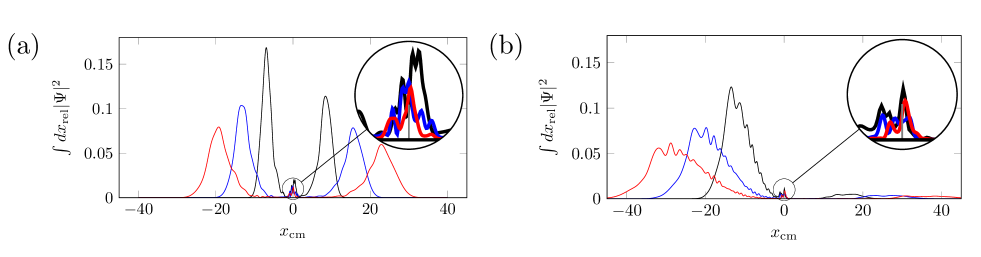
Figure 8: (a) Wave-function for $t=0.5$ (black), $t=0.8$ (blue), and $t=1.1$ (red). The inset shows the part of the wave-packet which is trapped at the mirror. The parameters are the same as in Fig. 5. (b) Wave-function for $t=1$ (black), $t=1.5$ (blue), and $t=2$ (red). We selected the parameters $V_{\mathrm{m}}^{1,2}=20$, $\Omega=5$, $P=8$, and $\sigma=1/2$.

V WKB analysis

It is possible to analyze the Schrödinger equation (7) within a WKB approximation which will give a qualitative understanding for the occurence of the resonances. For this, we turn to the time-independent version of (7) using the ansatz $\mathbf{f}=\mathbf{f}_{E}e^{-iEt}$. After reintroducing $\hbar$, the time-independent Schrödinger equation has the form

$$E\,\mathbf{f}_{E}=-\hbar^{2}\frac{d\mathbf{f}_{E}}{dx^{2}_{\mathrm{cm}}}+(\hat{\epsilon}+\hat{V})\mathbf{f}_{E}\,.$$ (10)

We choose the ansatz

$$\mathbf{f}_{E}=\hat{M}e^{i\frac{\hat{S}_{0}}{\hbar}}\hat{A}\mathbf{v}\,,$$ (11)

where $\mathbf{v}=(0,...0,1,0,...,0)$ is a unit vector and $\hat{M}$, $\hat{A}$ and $\hat{S}_{0}$ are matrices. Up order unity we obtain a first-order differential equation for $\hat{S}_{0}$,

$$\left(\frac{d\hat{S}_{0}}{dx_{\mathrm{cm}}}\right)^{2}+\hat{M}^{-1}(\hat{\epsilon}+\hat{V})\hat{M}=E.$$ (12)

If we demand that the matrix $\hat{S}_{0}$ is diagonal, the matrix $\hat{M}^{-1}(\hat{\epsilon}+\hat{V})\hat{M}=\hat{V}_{D}$ has to be of diagonal form which in turn determines $\hat{M}$. Up to order $\hbar$, we obtain as a condition for $\hat{A}$

$$0= 2e^{-i\frac{\hat{S}_{0}}{\hbar}}\left(\frac{d\hat{S}_{0}}{dx_{\mathrm{cm}}}\right)^{-1}\hat{M}^{-1}\frac{d\hat{M}}{dx_{\mathrm{cm}}}\left(\frac{d\hat{S}_{0}}{dx_{\mathrm{cm}}}\right)e^{i\frac{\hat{S}_{0}}{\hbar}}$$

$$+2\left(\frac{d\hat{A}}{dx_{\mathrm{cm}}}\right)\hat{A}^{-1}+\frac{d^{2}\hat{S}_{0}}{dx_{\mathrm{cm}}^{2}}\,.$$ (13)

Figure 9: Effective potentials for $\Omega=0.1$ and $V=10$. (a) $V_{-}$ has no resonance since the local minimum is too shallow.
(b) $V_{+}$ has two resonances which are related to a symmetric and an antisymmetric state. The inset shows the energy splitting of the states.

If the potential matrix were spatially constant, the first term in equation (V) would vanish. For simplicity we assume that the potential matrix $\hat{V}$ variies slowly such that we can neglect $d\hat{M}/dx_{\mathrm{cm}}$. The WKB solution takes then the form

$$\mathbf{f}^{\mathrm{WKB}}_{E}(x_{\mathrm{cm}}) =\hat{M}(x_{\mathrm{cm}})\mathbf{g}^{\mathrm{WKB}}_{E}(x_{\mathrm{cm}})$$ (14)

with

$$\mathbf{g}^{\mathrm{WKB}}_{E}(x_{\mathrm{cm}})=\frac{\exp\left(\pm i\int_{0}^{x_{\mathrm{cm}}}dx_{\mathrm{cm}}^{\prime}\sqrt{E-\hat{V}_{D}(x_{\mathrm{cm}}^{\prime})}\right)}{\sqrt{E-\hat{V}_{D}(x_{\mathrm{cm}})}}\mathbf{v}\,.$$ (15)

Here we assumed that the the energy is larger than the entries of the potential matrix. Otherwise one has exponential increasing or decreasing WKB-solutions.

In the following, we limit our considerations to the modes $n=0$ and $n=2$ and assume a symmetric scattering process with $V_{\mathrm{m}}^{1}=V_{\mathrm{m}}^{2}=V>0$. Therefore, we assume that the excitations related to $n=4,6,...$ can be disregarded. Within the order of approximation, we have two modes

$$\mathbf{g}^{\mathrm{WKB}}_{E,-}(x_{\mathrm{cm}})=g^{\mathrm{WKB}}_{-}(x_{\mathrm{cm}})\begin{pmatrix}0\\ 1\end{pmatrix}$$ (16)

and

$$\mathbf{g}^{\mathrm{WKB}}_{E,+}(x_{\mathrm{cm}})=g^{\mathrm{WKB}}_{+}(x_{\mathrm{cm}})\begin{pmatrix}1\\ 0\end{pmatrix}$$ (17)

which are WKB-solutions of the eigenvalue equations

$$-\frac{d^{2}g_{\pm}}{dx_{\mathrm{cm}}^{2}}+V_{\pm}(x_{\mathrm{cm}})g_{\pm}=Eg_{\pm}\,.$$ (18)

The potentials are given by

$$V_{\pm} =\frac{1}{2}\bigg{[}\epsilon_{0}+\epsilon_{2}+4V(\phi_{0}^{2}+\phi_{2}^{2})$$

$$\pm\sqrt{[\epsilon_{0}-\epsilon_{2}+4V(\phi_{0}^{2}-\phi_{2}^{2})]^{2}+64V^{2}\phi_{0}^{2}\phi_{2}^{2}}\bigg{]}\,.$$ (19)

For positive $V$, we have $V_{\pm}(x_{\mathrm{cm}})>V_{\pm}(x_{\mathrm{cm}}\rightarrow\pm\infty)$ such that bound states are not possible but resonances can appear. Indeed, $V_{-}$ has one local minimum whereas $V_{+}$ has two local minima, see Fig. 9. If the scattering potential is much larger than the internal level spacing, $V\gg\Omega^{1/2}$, the potentials can be approximated by

$$V_{-}(x_{\mathrm{cm}})=\frac{\Omega(11-4\Omega x_{\mathrm{cm}}^{2}+4\Omega^{2}x_{\mathrm{cm}}^{4})}{3-4\Omega x_{\mathrm{cm}}^{2}+4\Omega^{2}x_{\mathrm{cm}}^{4}}$$ (20)

and

$$V_{+}(x_{\mathrm{cm}})=\frac{2\sqrt{\Omega}Ve^{-\Omega x_{\mathrm{cm}}^{2}}}{\sqrt{\pi}}(3-4\Omega x_{\mathrm{cm}}^{2}+4\Omega^{2}x_{\mathrm{cm}}^{4})\,.$$ (21)

For the potential $V_{-}$ (see Fig. 9 (a)), we find that the local minimum is too shallow to support a resonance. In contrary, the potential $V_{+}$ (see Fig. 9 (a)) supports for $V\gg\Omega^{1/2}$ two resonances which correspond to a symmetric and an anti-symmetric state. The energies are given by

$$E^{S/A}_{\mathrm{res}}=V_{\mathrm{min}}+\omega\pm\frac{\omega}{\pi}e^{-\alpha}-\frac{i\omega}{\pi}e^{-2\beta}\,,$$ (22)

where $V_{\mathrm{min}}\approx 1.20\,\Omega^{1/2}V$ and $\omega\approx 2.14\,\Omega^{3/4}V^{1/2}$ are the value of the potential $V_{+}$ at the local minima and the stiffness, respectively. Furthermore, the exponent $\alpha\approx-1.20+1.22\,\Omega^{-1/4}V^{1/2}$ determines the tunnel coupling between the minima and the exponent $\beta\approx-1.91+0.45\,\Omega^{-1/4}V^{1/2}$ determines the decay rate of the resonance.

VI Conclusion.

We have shown with a simple model that resonances can occur in the scattering process of a composite system. In particular we studied the splitting of a wave-packet by a potential which mimics a partially silvered mirror. Depending on the particular system-mirror we found long-living and short-living resonances. If both particles interact with the mirror, it is possible that the composite system is trapped at the mirror for a finite time. We want to emphasize that these resonances occur due to the interaction between a purely repulsive potential (mirror) and the internal attractive potential. In contrast, resonances and even bound states would not be surprising for an attractive mirror potential.

When internal degrees of freedom become excited during the scattering process, partial which-path-information can be obtained since the modes of the reflected and the transmitted wave-packet are populated differently. Our findings should be of importance in the context of state preparation of mesoscopic objects or double-slit experiments with composite systems. In particular, the excitations of internal degrees of freedom have to be taken into account when the superposition principle is tested on a macroscopic scale, e.g. with optical trapped microspheres KHKRSJA12 ; AKM14 .

Appendix

In the following we give a brief introduction into the method of complex scaling which allows to determine the position of resonances.

Resonances result from imposing outgoing boundary conditions on the eigenfunctions of a time-independent Hamiltonian. For our discussion, we consider the Hamiltonian of a particle which moves in a potential $V(\hat{x})$. The Hamiltonian is given by

$$\hat{H}=\hat{p}^{2}+\hat{V}(\hat{x})$$ (23)

and the asymptotic form of a general solution to the time-independent Schrödinger equation takes the form

$$\psi_{k}(x\rightarrow+\infty) =A_{+}(k)e^{-ikx}+B_{+}(k)e^{+ikx}$$ (24)

$$\psi_{k}(x\rightarrow-\infty) =A_{-}(k)e^{+ikx}+B_{-}(k)e^{-ikx}\,.$$ (25)

Here we assumed that the potential vanishes for $x\rightarrow\pm\infty$ and $k$ is the asymptotic momentum of the particle. When the amplitude of the incoming wave, $A_{\pm}$, vanishes at $k=k_{\mathrm{res}}$, the system exhibits a bound state (for $\mathrm{Re}(\mathrm{res})>0$ and $\mathrm{Im}(\mathrm{res})=0$) or a resonance (for $\mathrm{Re}(\mathrm{res})>0$ and $\mathrm{Im}(\mathrm{res})<0$). The imaginary part of the corresponding energy, $E_{\mathrm{res}}=k_{\mathrm{res}}^{2}$ is the lifetime of the resonance. The complex wave vector is given by $k_{\mathrm{res}}=|k_{\mathrm{res}}|e^{-i\phi}$, where

$$\phi=-\frac{1}{2}\mathrm{arctan}\left(\frac{\mathrm{Im}(E_{\mathrm{res}})}{\mathrm{Re}(E_{\mathrm{res}})}\right)$$ (26)

lies in the range $0<\phi<\pi/2$ for a resonant eigenfunction. Asymptotically, the eigenfunctions adopt the form

$$\psi_{k_{\mathrm{res}}}(x\rightarrow+\infty) =B_{+}(k_{\mathrm{res}})e^{i|k_{\mathrm{res}}|\cos(\phi)x}e^{|k_{\mathrm{res}}|\sin(\phi)x}$$ (27)

$$\psi_{k_{\mathrm{res}}}(x\rightarrow-\infty) =B_{-}(k_{\mathrm{res}})e^{-i|k_{\mathrm{res}}|\cos(\phi)x}e^{-|k_{\mathrm{res}}|\sin(\phi)x}\,.$$ (28)

Since the functions diverge for $x\rightarrow\pm\infty$ they are not eigenfunctions of an hermitian operator. Complex scaling is based on a scaling transformation of the time-independent Schrödinger equation such that the (transformed) resonant eigenfunction becomes square-integrable. Then the resonant eigenenergies can be determined from an eigenvalue equation of the transformed (non-hermitian) Hamiltonian. A general scaling operator is of the form

$$\hat{S}=\sqrt{\eta}e^{\ln\eta x\frac{\partial}{\partial x}}$$ (29)

and transforms a wave-function according to

$$\hat{S}\psi(x)=\sqrt{\eta}\psi(\eta x)\,.$$ (30)

Choosing $\eta=e^{i\theta}$, the coordinate is rotated into the complex plane. The Hamiltonian is transformed according to

$$\hat{H}(\theta)=\hat{S}\hat{H}\hat{S}^{-1}=\hat{p}^{2}e^{-2i\theta}+\hat{V}(\hat{x}e^{i\theta})\,,$$ (31)

where we assumed that the potential can be analytically continued into the complex plane. When the system has no energy threshold, the energies of the continuum states are $E_{\mathrm{cont}}=k^{2}$. The states themselves are combinations of ingoing and outgoing waves,

$$\psi^{\mathrm{cont}}_{k}(x)=A(k)^{-ikx}+B(k)^{ikx}$$ (32)

and will be transformed under complex scaling to

$$\psi^{\mathrm{cont}}_{k}(xe^{i\theta})=A(k)^{-ikxe^{i\theta}}+B(k)^{ikxe^{i\theta}}\,.$$ (33)

The only solutions which do not diverge have the wave vectors $k=|k|e^{-i\theta}$. Thus, the continuum energies are rotated into the complex plane according to $E_{\mathrm{cont}}(\theta)=E_{\mathrm{cont}}e^{-2i\theta}$. Since we assumed that the system has no energy threshold, the branch point of the rotated continuum is the origin of the complex energy plane.

A resonant wavefunction with the asymptotics (27) and (28) becomes square-integrable when

$$\theta\geq\phi\,.$$ (34)

The corresponding eigenvalue $E_{\mathrm{res}}$ of the analytical continued (non-hermitian) Hamiltonian $H(\theta)$ appears as isolated point in the spectrum when the condition (34) is satisfied. It can be shown that $E_{\mathrm{res}}$ is locally independent of $\theta$ although the corresponding transformed eigenfunction $\psi_{k_{\mathrm{res}}}(xe^{i\theta})$ varies with $\theta$.

For the analysis of the two-particle bound system, it is necessary to generalize the discussion. Due to the internal structure of the bound system, there are infinitely many coupled mode functions $f_{n}$. Each function $f_{n}$ corresponds to an energy threshold $\epsilon_{n}$ and has the asymptotic form

$$f_{n,k}(x\rightarrow+\infty)= A_{n,+}(k)e^{-i\sqrt{k^{2}-\epsilon_{n}}x}$$

$$+B_{n,+}(k)e^{+i\sqrt{k^{2}-\epsilon_{n}}x}$$ (35)

$$f_{n,k}(x\rightarrow-\infty)= A_{n,-}(k)e^{+i\sqrt{k^{2}-\epsilon_{n}}x}$$

$$+B_{n,-}(k)e^{-i\sqrt{k^{2}-\epsilon_{n}}x}\,.$$ (36)

At a resonance, at least one of the mode functions satisfies the outgoing boundary condition

$$f_{n,k_{\mathrm{res}}}(x_{\mathrm{cm}})\sim\begin{cases}e^{i\sqrt{k_{\mathrm{res}}^{2}-\epsilon_{n}}x_{\mathrm{cm}}}&\text{ for }x\rightarrow\infty\\ e^{-i\sqrt{k_{\mathrm{res}}^{2}-\epsilon_{n}}x_{\mathrm{cm}}}&\text{ for }x\rightarrow-\infty\,.\end{cases}$$ (37)

The asymptotic form of this component of the wavefunction reads

$$f_{n,k_{\mathrm{res}}}(x_{\mathrm{cm}}\rightarrow\infty) \sim e^{ia_{n}x_{\mathrm{cm}}}e^{b_{n}x_{\mathrm{cm}}}\rightarrow\infty$$ (38)

which diverges for large $x_{\mathrm{cm}}$ since

$$a_{n} =|E_{\mathrm{res}}-\epsilon_{n}|^{1/2}\cos(\phi_{n})$$ (39)

$$b_{n} =|E_{\mathrm{res}}-\epsilon_{n}|^{1/2}\sin(\phi_{n})>0$$ (40)

$$\phi_{n} =\frac{1}{2}\mathrm{arctan}\left(\frac{\mathrm{Im}(E_{\mathrm{res}})}{\mathrm{Re}(E_{\mathrm{res}})-\epsilon_{n}}\right)\,.$$ (41)

Acting with a complex-scaling operator on the wavefunction which transforms $x_{\mathrm{cm}}\rightarrow e^{i\theta}x_{\mathrm{cm}}$, we find that the wavefunction becomes square integrable for angles $\theta\geq\phi_{n}$. The continuum energies are rotated into the complex and start at the branch points $\epsilon_{n}$,

$$E_{\mathrm{cont}}(\theta)=\epsilon_{n}+(E_{\mathrm{cont}}-\epsilon_{n})e^{-2i\theta}\,.$$ (42)

References

• (1) J. Summhammer, G. Badurek, H. Rauch, U. Kischko and A. Zeilinger, Phys. Rev. A 27 2523 (1983).
• (2) R. Rouse, S. Han, and J. E. Lukens, Phys. Rev. Lett. 75, 1614 (1995).
• (3) J. Clarke, A. N. Cleland, M. H. Devoret, D. Esteve and J. M. Martinis, Science 239, 992 (1998).
• (4) P. Silvestrini, V. G. Palmieri, B. Ruggiero and M. Russo, Phys. Rev. Lett. 79, 3046 (1997).
• (5) Y. Nakamura, Y. A. Pashkin and J. S. Tsai, Nature 398, 786 (1999).
• (6) J. R. Friedman, M. P. Sarachik, J. Tejada and R. Ziolo, Phys. Rev. Lett. 76, 3830 (1996).
• (7) E. del Barco, N. Vernier, J. M. Hernandez, J. Tejada, E. M. Chudnovsky, E. Molins and G. Bellessa, Europhys. Lett. 47 722 (1999).
• (8) W. Wernsdorfer, E. Bonet Orozco, K. Hasselbach, A. Benoit, D. Mailly, O. Kubo, H. Nakano and B. Barbara, Phys. Rev. Lett. 79, 4014 (1997).
• (9) C. Monroe, D. M. Meekhof, B. E. King, D. J. Wineland, Science 272, 1131 (1996).
• (10) M. Brune, E. Hagley, J. Dreyer, X. Maître, A. Maali, C. Wunderlich, J. M. Raimond, and S. Haroche Phys. Rev. Lett. 77, 4887 (1996).
• (11) M. Arndt, O. Nairz, J. Vos-Andreae, C. Keller, G. van der Zouw, and A. Zeilinger, Nature 401, 680 (1999).
• (12) S. Eibenberger, S. Gerlich, M. Arndt, M. Mayor, and J. Tüxen, Phys. Chem. Chem. Phys. 15, 14696 (2013).
• (13) O. Romero-Isart, L. Clemente, C. Navau, A. Sanchez, and J. I. Cirac, Phys. Rev. Lett. 109, 147205 (2012).
• (14) M. Schlosshauer, Decoherence and the Quantum-to-Classical Transition (Springer, Berlin, 2007).
• (15) W. H. Zurek, Rev. Mod. Phys. 75, 715 (2003).
• (16) Y. Chen, J. Physi. B: Atomic, Molecular and Optical Physics, 46, 104001 (2013).
• (17) A. Bassi, K. Lochan, S. Satin, T. P. Singh and H. Ulbricht, Rev. Mod. Phys. 85, 471 (2013).
• (18) A. Bassi and G. Ghirardi, Phys. Rep. 379 257 (2003).
• (19) G. C. Ghirardi, P. Pearle and A. Rimini, Phys. Rev. A 42 78 (1990).
• (20) O. Romero-Isart, Phys. Rev. A 84 052121 (2011).
• (21) R. Kaltenbaek, G. Hechenblaikner, N. Kiesel, O. Romero-Isart. K. C. Schwab, U. Johann, and M. Aspelmeyer, Exp. Astron.  34 123 (2012).
• (22) M. P. Blencowe, Phys. Rev. Lett. 111, 021302 (2013).
• (23) C. Anastopoulos, B. L. Hu, Class. Quantum Grav. 30 165007 (2013).
• (24) H.-P. Breuer, E. Göklü, C. Lämmerzahl, Class. Quantum Grav. 26 105012 (2009).
• (25) F. Suzuki and F. Queisser, J. Phys.: Conf. Ser. 626, 012039 (2015).
• (26) C. Gooding and W. G. Unruh, Phys. Rev. D 90, 044071 (2014).
• (27) D. Jaksch, C. Bruder, J. I. Cirac, C. W. Gardiner, and P. Zoller, Phys. Rev. Lett. 81, 3108 (1998).
• (28) N. Moiseyev, Phys. Rep. 302 212 (1998).
• (29) N. Moiseyev, P. R. Certain, F. Weinhold, Molecular Physics 36 1613 (1978).
• (30) B. Simon, Int. J. Quant. Chem. 14 529 (1978).
• (31) M. Reed and B. Simon, Methods of modern mathematical physics, academic press (1978).
• (32) N. Moiseyev, Non-hermitian quantum mechanics, Cambridge University Press (2011).
• (33) M. Aspelmeyer, T. J. Kippenberg and F. Marquardt, Rev. Mod. Phys. 86, 1391 (2014).