KUNS-2547

Random volumes from matrices

Masafumi Fukuma, Sotaro Sugishita and Naoya Umeda

Department of Physics, Kyoto University, Kyoto 606-8502, Japan

We propose a class of models which generate three-dimensional random volumes, where each configuration consists of triangles glued together along multiple hinges. The models have matrices as the dynamical variables and are characterized by semisimple associative algebras $\mathcal{A}$. Although most of the diagrams represent configurations which are not manifolds, we show that the set of possible diagrams can be drastically reduced such that only (and all of the) three-dimensional manifolds with tetrahedral decompositions appear, by introducing a color structure and taking an appropriate large $N$ limit. We examine the analytic properties when $\mathcal{A}$ is a matrix ring or a group ring, and show that the models with matrix ring have a novel strong-weak duality which interchanges the roles of triangles and hinges. We also give a brief comment on the relationship of our models with the colored tensor models.

1 Introduction

String theory is a strong candidate for a unified theory including quantum gravity. However, it still does not have a constructive, nonperturbative definition. The main reason is the lack of our understanding on the real fundamental dynamical variables of string theory. In fact, since the advent of D-branes and the discovery of string dualities, the idea has widely spread that the fundamental dynamical variables need not be strings and can be other types of extended objects.

M-theory [1] is a description of string theory, where membranes are believed to play an important role. The worldvolume theory of membranes is equivalent to a three-dimensional gravity theory, where the target space coordinates of an embedded membrane are expressed as scalar fields in three-dimensional worldvolume (see [3] for a review). However, the analytic understanding of three-dimensional quantum gravity is still not sufficient, as compared to that of two-dimensional quantum gravity [4, 5, 6].

Here, the roles played by matrix models in string theory should be suggestive, where the Feynman diagrams of matrix models are interpreted as triangular (or polygonal) discretization of string worldsheets (see [7, 8] for reviews). Furthermore, by introducing the degrees of freedom corresponding to matters on worldsheets or by considering a matrix field theory, one can define various kinds of string theory in terms of matrix models [9]. The $1/N$ expansion of matrix models, where $N$ is the size of matrix, corresponds to the genus expansion of string worldsheets as in [10]. Moreover, the double scaling limit enables us to study the nonperturbative aspects of string theory [11, 12, 13, 14, 15, 16] as well as their integrable structure [17, 18, 19].

Tensor models [20, 21, 22] or group field theory [23, 24] are natural generalizations of matrix models to three (and higher) dimensions. For three-dimensional models, the perturbative expansion generates random tetrahedral decompositions of three-dimensional objects. Unlike the two-dimensional case, however, these objects are not always manifolds or not even pseudomanifolds. Recently the situation was drastically improved by the colored tensor models (see, e.g., [25] for a review). It is shown that the colored tensor models admit a large $N$ expansion and the leading contributions represent higher dimensional sphere [26, 27]. Moreover, it is claimed that one can take a double scaling limit in the tensor models [28, 29]. Thus, the colored tensor models give a fascinating formulation of higher dimensional quantum gravity. Nevertheless, the analytic treatment of tensor models is still not so easy as that of matrix models. For example, tensors cannot be diagonalized as matrices can, and an analogue of saddle point method has not been found yet.

In the present paper, we propose a new class of models which generate three-dimensional random volumes, by regarding each random diagram as a collection of triangles glued together along multiple hinges as in [30]. Our models have real symmetric matrices as the dynamical variables and are characterized by semisimple associative algebras $\mathcal{A}$. Although most of the diagrams represent configurations which are not manifolds, we show that the set of possible diagrams can be drastically reduced such that only (and all of the) three-dimensional manifolds with tetrahedral decompositions appear, by introducing a color structure and taking an appropriate limit of parameters existing in the models.

Since our models are written with matrices, there should be a chance that various techniques in matrix models can be applied and the dynamics of random volumes can be understood more analytically. We show that our models have a novel strong-weak duality which interchanges the roles of triangles and hinges when $\mathcal{A}$ is a matrix ring. This duality may suggest the analytic solvability of the models.

This paper is organized as follows. In section 2, we first define our models and show that the models are characterized by semisimple associative algebras $\mathcal{A}$. We then give a few examples of the Feynman diagrams, and show that some diagrams are not manifolds. From the examples, we deduce a strategy to restrict the models so that only (and all of the) three-dimensional manifolds are generated. This strategy is implemented in section 3, where matrix rings are taken as the defining associative algebras. We explicitly construct models that generate only manifolds as Feynman diagrams, by introducing a color structure to the models and letting the associative algebras have centers whose dimensions play the role of free parameters. In section 4 we investigate the models where $\mathcal{A}$ is set to be a group ring $\mathbb{R}[G]$, and demonstrate how the models depend on details of the group structure of $G$. Section 5 is devoted to conclusion and discussions. We list some of the future directions for further study of the models, and give a brief comment on the relationship of our models with the colored tensor models.

2 The models

In this section we define a class of models which have matrices as the dynamical variables and generate Feynman diagrams consisting of triangles glued together along multiple hinges. We show that the models can be defined by semisimple associative algebras. We then give a few examples of the Feynman diagrams, and show that some diagrams are not manifolds. We will conclude the section by giving a strategy to restrict the models so that only three-dimensional manifolds are generated. This strategy will be implemented in the next section, where matrix rings are taken as the defining associative algebras.

2.1 General structure

We first explain the diagrams we are concerned with and give the rule to assign a Boltzmann weight to each diagram. We then write down the action which generates such diagrams as Feynman diagrams.

We consider a set of diagrams, $\{\gamma\}$, consisting of triangles glued together along multiple hinges as in [30]. In order to assign a Boltzmann weight to diagram $\gamma$, we first decompose $\gamma$ to a set of triangles and a set of multiple hinges (see Fig. 1).

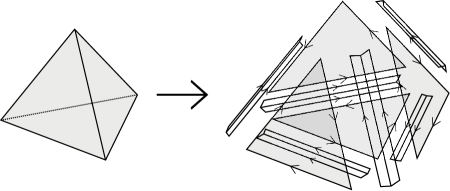
Figure 1: Decomposition of a three-dimensional diagram to triangles and hinges.

For each edge of a triangle, we draw an arrow and assign an index from a finite set $\{I\}$. We repeat the same procedure for the hinges. We then assign the real numbers $C^{IJK}$ and $Y_{I_{1}\ldots I_{k}}$ to the indexed triangles and hinges, respectively, as in Fig. 2.

Figure 2: Triangles and hinges.

We require that $C^{IJK}$ and $Y_{I_{1}\ldots I_{k}}$ be cyclically symmetric.

Then, we glue the triangles and hinges to reconstruct the original diagram in such a way that the identified edges have the same index. In doing this, there may appear the case where the arrows of a triangle and a hinge have opposite directions. To treat such cases, we introduce a tensor $T_{I}^{\phantom{I}J}$ which reverses the direction of an arrow (see Fig. 3).

Figure 3: Tensor $T_{I}^{\,\,J}$. It changes the direction of arrow.

Note that the tensor $T=(T_{I}^{\phantom{I}J})$ should be involutory because the direction of an arrow comes back to the original one after $T_{I}^{\phantom{I}J}$ is applied twice:

$$T_{I}^{\phantom{I}K}T_{K}^{\phantom{K}J}=\delta_{I}^{\phantom{I}J}.$$ (2.1)

Furthermore, the following relations should hold since a hinge (or a triangle) whose arrows are all flipped is equivalent to a hinge (or a triangle) with indices in reverse order:

$$T_{I_{1}}^{\phantom{I_{1}}J_{1}}\ldots T_{I_{k}}^{\phantom{I_{k}}J_{k}}Y_{J_{1}\ldots J_{k}} =Y_{I_{k}\ldots I_{1}},$$ (2.2)

$$C^{LMN}\,T_{L}^{\phantom{L}I}T_{M}^{\phantom{M}J}T_{N}^{\phantom{N}K} =C^{KJI}.$$ (2.3)

We define the Boltzmann weight $w(\gamma)$ of diagram $\gamma$ to be the product of $C^{IJK}$ and $Y_{I_{1}\ldots I_{k}}$ followed by the summation over the indices on the edges:

$$w(\gamma)=\frac{1}{S(\gamma)}\,\sum_{\{I_{e}\}}\prod_{f:\,{\rm triangle}}C^{IJK}(f)\,\prod_{h:\,{\rm hinge}}Y_{I_{1}\ldots I_{k}}(h)\,.$$ (2.4)

Here, $I_{e}$ are the indices on the edges, and $S(\gamma)$ is the symmetry factor of the diagram. The indices in $C^{IJK}$ and $Y_{I_{1}\ldots I_{k}}$ are contracted when the corresponding edges are identified (with $T_{I}^{\phantom{I}J}$ inserted appropriately if necessary).

The above diagrams with the prescribed Boltzmann weights can be generated as Feynman diagrams from the action

$$S[A,B]=\frac{1}{2}A_{I}B^{I}-\frac{\lambda}{6}C^{IJK}A_{I}A_{J}A_{K}-\sum_{k\geq 2}^{\infty}\frac{\mu_{k}}{2k}B^{I_{1}}\cdots B^{I_{k}}Y_{I_{1}\ldots I_{k}},$$ (2.5)

where the dynamical variables $A_{I}$ and $B^{I}$ satisfy the relations

$$A_{I}=T_{I}^{\phantom{I}J}A_{J},\qquad B^{I}=B^{J}T_{J}^{\phantom{J}I}.$$ (2.6)

We have included the coupling constants $\lambda$ and $\mu_{k}$ $(k\geq 2)$ to count the numbers of triangles and $k$-hinges, respectively. In order to specify the directions of arrows, the index line will be a double line by setting index $I$ to be double index $I=(i,j)$.

It may be already clear, but we here explain how the action generates the diagrams we are concerned with. There are two kinds of interaction terms, one corresponding to triangles $C^{IJK}$ and the other to $k$-hinges $Y_{I_{1}\ldots I_{k}}$ $(k\geq 2)$. The kinetic term $(1/2)A_{I}B^{I}$ yields a propagator that glues an edge of a triangle and that of a hinge. Note that two triangles cannot be glued to each other without an intermediate hinge, and two hinges cannot be glued to each other without an intermediate triangle. In order to handle the case where the tensor $T_{I}^{\phantom{I}J}$ needs to be inserted, we should multiply every leg of interaction terms by the factor $\delta_{I}^{\phantom{I}J}+T_{I}^{\phantom{I}J}$. However, this is equivalent to inserting the projector $\bigl{(}\delta_{I}^{\phantom{I}J}+T_{I}^{\phantom{I}J}\bigr{)}/2$ in every propagator, which in turn is equivalent to requiring that the dynamical variables be invariant under the action of $T_{I}^{\phantom{I}J}$.

In summary, our model is characterized by the data $(C^{IJK},Y_{I_{1}\ldots I_{k}},T_{I}^{\phantom{I}J})$ that satisfy the constraints (2.1)–(2.3). In the next subsection we show that most of the constraints can be solved by considering semisimple associative algebras.

2.2 Algebraic construction

In this subsection, we give an algebraic construction of the model data $(C^{IJK},Y_{I_{1}\ldots I_{k}},T_{I}^{\phantom{I}J})$ (see [30] and also [32, 33] for a related idea).

Let $\mathcal{R}$ be a real semisimple associative algebra. That is, $\mathcal{R}$ is a linear space over $\mathbb{R}$ with multiplication (denoted by $\times$) that satisfies the associativity, $(B_{1}\times B_{2})\times B_{3}=B_{1}\times(B_{2}\times B_{3})$. If one introduces a basis $\{E_{I}\}$ as $\mathcal{R}=\bigoplus_{I}\mathbb{R}\,E_{I}$, the multiplication is expressed in the form $E_{I}\times E_{J}=Y_{IJ}^{\phantom{IJ}K}E_{K}$, where the structure constants $Y_{IJ}^{\phantom{IJ}K}$ satisfy the relations $Y_{IJ}^{\phantom{IJ}L}Y_{LK}^{\phantom{LK}M}=Y_{IL}^{\phantom{IL}M}Y_{JK}^{\phantom{JK}L}$ due to associativity. The $k$-hinge tensor $Y_{I_{1}\ldots I_{k}}$ can then be constructed from $Y_{IJ}^{\phantom{IJ}K}$ as

$$Y_{I_{1}\ldots I_{k}}\equiv Y_{I_{1}J_{1}}^{\phantom{I_{1}J_{1}}J_{k}}Y_{I_{2}J_{2}}^{\phantom{I_{2}J_{2}}J_{1}}\ldots Y_{I_{k}J_{k}}^{\phantom{I_{k}J_{k}}J_{k-1}}.$$ (2.7)

It is easy to see that $Y_{I_{1}\ldots I_{k}}$ are cyclically symmetric. The two-hinge tensor $Y_{IJ}$ is called the metric of $\mathcal{R}$ and will often be denoted by $G_{IJ}$; $G_{IJ}=Y_{IJ}=Y_{IK}^{\phantom{IK}L}Y_{JL}^{\phantom{JL}k}$. It is known [32] that the associative algebra $\mathcal{R}$ is semisimple (i.e., isomorphic to a direct sum of matrix rings) if and only if $G=(G_{IJ})$ has its inverse $G^{-1}\equiv(G^{IJ})$. The constraints (2.1) and (2.2) can be solved if there exists an involutory anti automorphism $T:\,\mathcal{R}\to\mathcal{R}$. In fact, the coefficients $T_{I}^{\phantom{I}J}$ in $T(E_{I})=T_{I}^{\phantom{I}J}\,E_{J}$ satisfies (2.1) when $T$ is involutory. Furthermore, when $T$ is an antiautomorphism: $T(E_{J}\times E_{I})=T(E_{I})\times T(E_{J})$, we have the relations $T_{I}^{\phantom{I}K}T_{J}^{\phantom{J}L}Y_{KL}^{\phantom{KL}N}=Y_{JI}^{\phantom{JI}M}T_{M}^{\phantom{M}N}$, which ensure (2.2) to hold.

Such an antiautomorphism can be naturally constructed when we set the index $I$ to be a double index $I=(i,j)$ $(i,j=1,\ldots,N)$ in order to assign arrows to the edges of triangles and hinges. To see this, we let $\mathcal{R}$ take the form

$$\mathcal{R} =\mathcal{A}\otimes\mathcal{\bar{A}},$$ (2.8)

where $\mathcal{A}$ and $\mathcal{\bar{A}}$ are linear spaces of the same dimension $N$. We fix an isomorphism from $\mathcal{A}$ to $\mathcal{\bar{A}}$ and denote it by $\sigma$. We assume that $\mathcal{A}$ is a semisimple associative algebra with multiplication $\times$. We introduce a multiplication (also denoted by $\times$) to $\mathcal{\bar{A}}$ such that $\sigma:\,\mathcal{A}\to\mathcal{\bar{A}}$ is an algebra anti automorphism, $\sigma(a\times b)=\sigma(b)\times\sigma(a)$ $(\forall a,\,b\in\mathcal{A})$. Then $\mathcal{R}=\mathcal{A}\otimes\mathcal{\bar{A}}$ naturally becomes an associative algebra as the tensor product of two associative algebras. The antiautomorphism $T:\,\mathcal{R}\to\mathcal{R}$ now can be defined such as to map an element $B=\sum b\otimes\bar{b}\in\mathcal{R}$ to

$$T(B)=\sum T(b\otimes\bar{b})\equiv\sum\sigma^{-1}(\bar{b})\otimes\sigma(b).$$ (2.9)

One can easily show that $T$ is certainly an antiautomorphism. We thus find that the constraints (2.1) and (2.2) can be solved by giving an associative algebra $\mathcal{A}$.

Note that $\mathcal{R}$ can also be thought of as the set of algebra endomorphisms of $\mathcal{A}$ by regarding $\mathcal{\bar{A}}$ as the dual linear space of $\mathcal{A}$ :

$$\mathcal{R} =\mathcal{A}\otimes\mathcal{\bar{A}}={\rm End}\,\mathcal{A}.$$ (2.10)

One then can also define an antiautomorphism $\bar{T}$ for the dual of $\mathcal{R}$, $\bar{\mathcal{R}}\equiv\bar{\mathcal{A}}\otimes\mathcal{A}$, such that the following relation holds:

$$\langle\,\bar{T}(A),\,T(B)\rangle=\langle A,\,B\rangle\quad(\forall A\in\bar{\mathcal{R}},\,\forall B\in\mathcal{R}),$$ (2.11)

where $\langle~{},~{}\rangle$ is the paring between $\bar{\mathcal{R}}$ (the dual of $\mathcal{R}$) and $\mathcal{R}$.

We rephrase the above construction in terms of the bases $\{e_{i}\}$ and $\{\bar{e}^{i}\}$ of $\mathcal{A}$ and $\mathcal{\bar{A}}$ :

$$\mathcal{A} =\bigoplus_{i=1}^{N}\mathbb{R}\,e_{i},\qquad\mathcal{\bar{A}}=\bigoplus_{i=1}^{N}\mathbb{R}\,\bar{e}^{i}.$$ (2.12)

We first represent the isomorphism $\sigma$ as

$$\sigma(e_{i})=\sigma_{ij}\,\bar{e}^{j},\qquad\sigma^{-1}(\bar{e}^{i})=\sigma^{ij}\,e_{j},$$ (2.13)

and write the structure constants of the multiplication on $\mathcal{A}$ as $e_{i}\times e_{j}=y_{ij}^{\phantom{ij}k}e_{k}$. Then those of $\mathcal{\bar{A}}$ (appearing in $\bar{e}^{i}\times\bar{e}^{j}=\bar{y}^{ij}_{\phantom{ij}k}\bar{e}^{k}$) are determined from the requirement of antihomomorphism, $\sigma(e_{i}\times e_{j})=\sigma(e_{j})\times\sigma(e_{i})$, to be

$$\bar{y}^{ij}_{\phantom{ij}k}=\sigma^{il}\sigma^{jm}y_{ml}^{\phantom{ml}n}\sigma_{nk}.$$ (2.14)

If we take the basis of $\mathcal{R}$ to be $E_{I}=E_{i}^{\phantom{i}j}=e_{i}\otimes\bar{e}^{j}$, then the structure constants $Y_{I_{1}I_{2}}^{\phantom{I_{1}I_{2}}I_{3}}$ are given by

$$Y_{I_{1}I_{2}}^{\phantom{I_{1}I_{2}}I_{3}}=Y_{i_{1}}^{\phantom{i_{1}}j_{1}}\!~{}_{i_{2}}^{\phantom{i_{2}}j_{2}}\!~{}^{i_{3}}_{\phantom{i_{3}}j_{3}}=y_{i_{1}i_{2}}^{\phantom{i_{1}i_{2}}i_{3}}\,\bar{y}^{j_{1}j_{2}}_{\phantom{j_{1}j_{2}}j_{3}},$$ (2.15)

from which the $k$-hinge tensor is given by

$$Y_{I_{1}\ldots I_{k}}=Y_{i_{1}}^{\phantom{i_{1}}j_{1}}\cdots\!~{}_{i_{k}}^{\phantom{i_{k}}j_{k}}=y_{i_{1}\ldots i_{k}}\,\bar{y}^{j_{1}\ldots j_{k}}$$ (2.16)

with

$$y_{i_{1}\ldots i_{k}} \equiv y_{i_{1}j_{1}}^{\phantom{i_{1}i_{1}}j_{k}}y_{i_{2}j_{2}}^{\phantom{i_{2}j_{2}}j_{1}}\ldots y_{i_{k}j_{k}}^{\phantom{i_{k}j_{k}}j_{k-1}},$$ (2.17)

$$\bar{y}^{i_{1}\ldots i_{k}} \equiv\bar{y}^{i_{1}j_{1}}_{\phantom{i_{1}i_{1}}j_{k}}\bar{y}^{i_{2}j_{2}}_{\phantom{i_{2}j_{2}}j_{1}}\ldots\bar{y}^{i_{k}j_{k}}_{\phantom{i_{k}j_{k}}j_{k-1}}=\sigma^{i_{1}j_{1}}\cdots\sigma^{i_{k}j_{k}}y_{j_{k}\ldots j_{1}}.$$ (2.18)

In particular, the metric of $\mathcal{R}$ takes the form

$$G_{I_{1}I_{2}}=G_{i_{1}}{}^{j_{1}}{}_{i_{2}}{}^{j_{2}}=g_{i_{1}i_{2}}\,\bar{g}^{j_{1}j_{2}},$$ (2.19)

where $g_{i_{1}i_{2}}$ and $\bar{g}^{j_{1}j_{2}}$ are the metrics of $\mathcal{A}$ and $\mathcal{\bar{A}}$, respectively; $g_{i_{1}i_{2}}\equiv y_{i_{1}k}^{\phantom{i_{1}k}\ell}\,y_{i_{2}\ell}^{\phantom{i_{1}\ell}k}$, $\bar{g}^{j_{1}j_{2}}=\bar{y}^{j_{1}k}_{\phantom{j_{1}k}\ell}\,\bar{y}^{j_{2}\ell}_{\phantom{i_{1}\ell}k}$. We easily see that $\mathcal{R}$ is semisimple if $\mathcal{A}$ is, because $G_{I_{1}I_{2}}$ has its inverse when $g_{i_{1}i_{2}}$ does (and so does $\bar{g}^{j_{1}j_{2}}$).

The antiautomorphism $T_{I}^{\phantom{I}J}$ is now expressed as $T(e_{i}\otimes\bar{e}^{j})\equiv\sigma^{-1}(\bar{e}^{j})\otimes\sigma(e_{i})=\sigma^{jk}\sigma_{il}\,e_{k}\otimes\bar{e}^{l}$, that is,

$$T_{I_{1}}^{\phantom{I_{1}}I_{2}}=T_{i_{1}}^{\phantom{i_{1}}j_{1}}{}^{i_{2}}_{\phantom{i_{2}}j_{2}}=\sigma_{i_{1}j_{2}}\,\sigma^{j_{1}i_{2}}.$$ (2.20)

For the dual algebra $\bar{\mathcal{R}}=\bar{\mathcal{A}}\otimes\mathcal{A}$, regarding $\{\bar{e}^{i}\}$ as the dual basis of $\{e_{i}\}$, we set a basis of $\bar{\mathcal{R}}$ to be $\bar{E}^{I}=\bar{E}^{i}_{\phantom{i}j}=\bar{e}^{i}\otimes e_{j}$, which leads to the pairing $\langle\bar{E}^{I_{1}},\,E_{I_{2}}\rangle=\delta^{i_{1}}_{i_{2}}\,\delta^{j_{2}}_{j_{1}}$. Then the antiautomorphism $\bar{T}$ on $\bar{\mathcal{R}}$ is expressed as $\bar{T}(\bar{E}^{I})\equiv\bar{E^{J}}(T^{-1})_{J}^{\phantom{J}I}=\bar{E^{J}}T_{J}^{\phantom{J}I}$.

The dynamical variables $A_{I}$ and $B^{I}$ in (2.5) can be regarded as elements of $\bar{\mathcal{R}}$ and $\mathcal{R}$, respectively:

$$A=A_{I}\bar{E}^{I}=A_{i}^{\phantom{i}j}\,\bar{e}^{i}\otimes e_{j}\in\bar{\mathcal{R}},\qquad B=B^{I}E_{I}=B^{i}_{\phantom{i}j}\,e_{i}\otimes\bar{e}^{j}\in\mathcal{R}.$$ (2.21)

The condition (2.6) is then expressed as $\bar{T}(A)=A$, $T(B)=B$. With these double indices, the action (2.5) is written as

$$S=\frac{1}{2}A_{i}^{\phantom{i}j}B^{i}_{\phantom{i}j}-\frac{\lambda}{6}C^{i\phantom{j}k\phantom{l}m\phantom{n}}_{\phantom{i}j\phantom{k}l\phantom{m}n}A_{i}^{\phantom{i}j}A_{k}^{\phantom{k}l}A_{m}^{\phantom{m}n}-\sum_{k\geq 2}\frac{\mu_{k}}{2k}B^{i_{1}}_{\phantom{i_{1}}j_{1}}\ldots B^{i_{k}}_{\phantom{i_{k}}j_{k}}y_{i_{1}\ldots i_{k}}\bar{y}^{j_{1}\ldots j_{k}},$$ (2.22)

where the tensor $C^{i\phantom{j}k\phantom{l}m\phantom{n}}_{\phantom{i}j\phantom{k}l\phantom{m}n}$ is arbitrary as long as it satisfies the condition (2.3). It is often convenient to use $A_{ij}\equiv\sigma_{jk}A_{i}^{\phantom{i}k}$, $B^{ij}\equiv B^{i}_{\phantom{i}k}\sigma^{kj}$, and $C^{ijklmn}\equiv C^{i\phantom{j^{\prime}}k\phantom{l^{\prime}}m\phantom{n^{\prime}}}_{\phantom{i}j^{\prime}\phantom{k}l^{\prime}\phantom{m}n^{\prime}}\sigma^{j^{\prime}j}\sigma^{l^{\prime}l}\sigma^{n^{\prime}n}$. Then the conditions (2.3) and (2.6) can be rewritten to the form where $\sigma$ does not appear:

$$C^{ijklmn}=C^{nmlkji},$$ (2.23)

$$A_{ij}=A_{ji},\quad B^{ij}=B^{ji}.$$ (2.24)

The action then becomes

$$S=\frac{1}{2}A_{ij}B^{ij}-\frac{\lambda}{6}C^{ijklmn}A_{ij}A_{kl}A_{mn}-\sum_{k\geq 2}\frac{\mu_{k}}{2k}B^{i_{1}j_{1}}\cdots B^{i_{k}j_{k}}y_{i_{1}\ldots i_{k}}y_{j_{k}\ldots j_{1}}.$$ (2.25)

Thus, a set of models can be defined by giving semisimple associative algebras $\mathcal{A}$ and the tensors $C^{ijklmn}$ satisfying (2.23). The isomorphism $\sigma:\,\mathcal{A}\to\bar{\mathcal{A}}$ can be taken arbitrarily and is regarded as a sort of gauge freedom in choosing the basis of $\mathcal{A}$ or $\bar{\mathcal{A}}$.

2.3 The Feynman rules

As stated in the last subsection, the tensor $C^{ijklmn}$ in (2.25) can be chosen arbitrarily as long as it satisfies the condition (2.23). In this paper, we set it to be

$$C^{ijklmn}=g^{jk}g^{lm}g^{ni},$$ (2.26)

which one can easily show to satisfy (2.23). Then the Feynman rules of the action (2.25) become

$${\rm propagator} :\ \begin{array}[]{l}\includegraphics[height=34.14322pt]{fig2-05.eps}\end{array}+\begin{array}[]{l}\includegraphics[height=34.14322pt]{fig2-06.eps}\end{array}\sim\langle A_{ij}B^{kl}\rangle=\delta_{i}^{\phantom{i}k}\delta_{j}^{\phantom{j}l}+\delta_{i}^{\phantom{i}l}\delta_{j}^{\phantom{j}k},$$ (2.29)

$${\rm triangle} :\ \begin{array}[]{l}\includegraphics[width=56.9055pt]{fig2-07.eps}\end{array}\sim\lambda\,g^{j_{1}i_{2}}\,g^{j_{2}i_{3}}\,g^{j_{3}i_{1}},$$ (2.31)

$$k :\ \begin{array}[]{l}\includegraphics[width=56.9055pt]{fig2-08.eps}\end{array}\sim\mu_{k}\,y_{i_{1}\ldots i_{k}}\,y_{j_{k}\ldots j_{1}}.$$-hinge (2.33)

Recall that the arrows are now expressed with double lines, and thus, when the first (or second) term of the propagator (2.29) is used the edges are glued in the same (or opposite) direction.

The free energy of this model takes the form

$$\log Z=\sum_{\gamma}\frac{1}{S(\gamma)}\,\lambda^{s_{2}(\gamma)}\Bigl{(}\prod_{k\geq 2}\mu_{k}^{s_{1}^{k}(\gamma)}\Bigr{)}\,\mathcal{F}(\gamma).$$ (2.34)

Here, the sum $\sum_{\gamma}$ is taken over all possible connected Feynman diagrams $\{\gamma\}$, and $S(\gamma)$ is the symmetry factor of diagram $\gamma$. $s_{2}(\gamma)$ is the number of triangles, and $s_{1}^{k}(\gamma)$ the number of $k$-hinges. $\mathcal{F}(\gamma)$ denotes the product of $y_{i_{1}\ldots i_{k}}$ and $g^{ij}$ with the indices contracted according to a given Wick contraction, and we call $\mathcal{F}(\gamma)$ the index function of diagram $\gamma$. We here regard two diagrams as being the same if the indices are contracted in the same manner. The numerical coefficients in the action (2.25) are chosen such that independent diagrams give only the symmetry factors to the free energy, by taking into account the symmetry (rotation and flip) of triangles and hinges. We stress that the free energy will have a different form from (2.34) if we make a different choice for $C^{ijklmn}$ other than (2.26).

We now show that the index function $\mathcal{F}(\gamma)$ can be expressed as the product of the contributions from two-dimensional  surfaces, each surface enclosing a vertex of diagram $\gamma$. To see this, we first note from the Feynman rules (2.29)–(2.33) that even a connected Feynman diagram generally gives disconnected networks of index lines. This is because each hinge has a pair of junction points as for index lines and two index lines out of the same edge of a hinge can enter two different hinges after passing through an adjacent triangle (see Fig. 4).

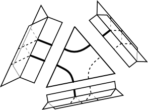
Figure 4: A part of index networks. Two index lines (depicted in bold lines) come out of the same edge of the left hinge and enter the right adjacent triangle. The upper index line then leaves the triangle and enters the upper hinge, while the lower index line enters the lower hinge.

We further note that the index lines on two different hinges can be connected (through an intermediate triangle) if and only if the hinges share the same vertex of $\gamma$. This means that the connected  index networks have a one-to-one correspondence to the vertices of $\gamma$. We thus find that the index function $\mathcal{F}(\gamma)$ of diagram $\gamma$ is the product of the contributions from connected index networks (each assigned to a vertex of $\gamma$) and has the form

$$\mathcal{F}(\gamma)=\prod_{v:\,\text{vertex of $\gamma$}}\zeta(v).$$ (2.35)

We also call $\zeta(v)$ the index function (more precisely, the index function of vertex $v$). Note that every connected index network takes the form of a polygonal decomposition of a closed surface (not necessarily a sphere and may include monogons or digons), where a $k$-valent junction (or $k$-junction) corresponds to a $k$-hinge where $k$ index lines meet (see Fig. 5).

Figure 5: Index network around a vertex. It represents a polygonal decomposition of a closed surface (not necessarily a sphere) around a vertex. A $k$-valent junction in the index network corresponds to a $k$-hinge in the original diagram, where $k$ index lines meet. A segment connecting two junctions in the index network corresponds to an intermediate triangle between two hinges.

We here make a few comments. The first comment is on the uniqueness in interpreting an index network as a polygonal decomposition of a closed surface. In fact, if one regards an index network simply as a wire frame (i.e., as a collection of segments), then it is not a unique procedure to assign polygonal faces in the frame such that the resulting configuration forms a closed surface. However, our index network is not simply a wire frame, and has the information on how the indices are contracted. We thus can uniquely assign faces to the holes of the index network by carefully following the contraction of indices. We will see in section 3 that the assignment is straightforward when models are given by matrix rings as the defining associative algebras.

The second comment is on the manifoldness of a diagram $\gamma$. Since there is a two-dimensional surface around each vertex of $\gamma$, we can say that there is a three-dimensional cone at each vertex, the base and apex of a cone being the connected index network around a vertex and the vertex itself, respectively. For example, if an index network has the topology of two-sphere $S^{2}$, then the corresponding cone is a 3-dimensional ball $B^{3}$. These cones characterize the neighborhoods of the vertices of the diagram $\gamma$. Note that $\gamma$ represents a three-dimensional (combinatorial) manifold if $\gamma$ gives a tetrahedral decomposition and the neighborhood of every vertex is homeomorphic to $B^{3}$. In section 3, by taking $\mathcal{A}$ to be a matrix ring and introducing a color structure to the models, we show that the set of possible Feynman diagrams can be drastically reduced such that only (and all of the) manifolds are generated.

2.4 Evaluation of diagrams

The index function $\mathcal{F}(\gamma)$ can be easily evaluated by deforming each connected index network with the use of the associativity of $y_{ij}^{\phantom{ij}k}=y_{ijl}\,g^{lk}$ [32]:

$$\begin{array}[]{l}\includegraphics[width=56.9055pt]{fig2-11.eps}\end{array}=y_{ij}^{\phantom{ij}l}y_{lkm}=y_{ilm}y_{jk}^{\phantom{jk}l}=\begin{array}[]{l}\includegraphics[height=56.9055pt]{fig2-12.eps}\end{array}.$$ (2.38)

In deformation there may appear two kinds of index loops:

$$\begin{array}[]{l}\includegraphics[width=113.81102pt]{fig2-13.eps}\end{array} =y_{ik}^{\phantom{ik}l}\,y_{jl}^{\phantom{jl}k}~{}~{}\Bigl{(}\,=g_{ij}=\begin{array}[]{l}\includegraphics[width=49.79231pt]{fig2-14.eps}\end{array}\Bigr{)},$$ (2.41)

$$\begin{array}[]{l}\includegraphics[width=113.81102pt]{fig2-15.eps}\end{array} =y_{ik}^{\phantom{ik}l}\,y_{lj}^{\phantom{lj}k}~{}~{}\Bigl{(}\,\equiv p_{ij}\Bigr{)}.$$ (2.43)

The former index loop diagram can be replaced by a single solid line, while the loop in the latter index diagram cannot be removed. Actually $p_{ij}$ (or more precisely, $p_{i}^{j}\equiv p_{ik}g^{kj}$) is a projector to the center of algebra $\mathcal{A}$, $Z(\mathcal{A})$, as can be checked easily [32]. If a given connected index network does not produce a projector $p_{ij}$ in the process of deformation, the index network can always be deformed to a single circle after repeatedly using (2.38) and (2.41) and gives the value $g_{ij}g^{ij}=N$, where $N$ is the dimension of $\mathcal{A}$. On the other hand, if a given connected index network admits the appearance of a projector $p_{ij}$, the value of the index network is generally less than $N$.

Note that the two deformations (2.38) and (2.41) are actually the local moves of two-dimensional surfaces. Therefore, the index function $\zeta(v)$ of vertex $v$ gives a two-dimensional topological invariant defined by the associative algebra $\mathcal{A}$ [32], and thus has the form $\zeta(v)=\mathcal{I}_{g(v)}$, where $g(v)$ is the genus of the network. Thus the index function of diagram $\gamma$ is expressed as

$$\mathcal{F}(\gamma)=\prod_{v:\,\text{vertex}}\zeta(v)=\prod_{v:\,\text{vertex}}\mathcal{I}_{g(v)}.$$ (2.44)

2.5 Examples

In this subsection we give a few examples of the diagrams generated in our models. If our aim is to apply the models to three-dimensional gravity, we should be able to assign three-dimensional volume to each diagram, and thus it is preferable that the diagrams can be regarded as collections only of tetrahedra. However, as we see in the examples below, there arise a lot of undesired diagrams. We will show in the next section that such undesired diagrams can be automatically excluded by taking specific associative algebras and modifying the form (2.26), with an appropriate limit of parameters.

2.5.1 Diagrams representing tetrahedral decompositions of manifolds

First we consider a diagram which represents a tetrahedral decomposition of three-dimensional sphere $S^{3}$ (see Fig. 6). This is the boundary of the so-called 5-cell or a 4-simplex and can be constructed from five tetrahedra.

Figure 6: A decomposition of $S^{3}$ with five tetrahedra. The tetrahedra are glued together at their faces so that each of the points $1,\ldots,5$ represents a single vertex.

Note that the diagram has ten triangles, ten 3-hinges and five vertices. All the index networks around vertices have the same topology and give triangular decompositions of $S^{2}$ as in Fig. 7. Thus, the neighborhood of each vertex is homeomorphic to $B^{3}$.

Figure 7: A contraction of indices around a vertex. This represents a triangular decomposition of $S^{2}$ and gives the value $N$.

Since every index network can be deformed to a single circle, the index function of each vertex takes the value $N$; $\zeta(v)=N=\mathcal{I}_{g(v)=0}$. Thus, the contribution from this diagram to the free energy is given by

$$\frac{1}{S}\,\lambda^{10}\mu_{3}^{10}\,(\mathcal{I}_{g=0})^{5}=\frac{1}{S}\,\lambda^{10}\mu_{3}^{10}\,N^{5},$$ (2.45)

where $S$ is the symmetry factor of the diagram.

The next example is a diagram which represents a tetrahedral decomposition of three-dimensional torus $T^{3}$ (see Fig. 8).

Figure 8: A tetrahedral decomposition of $T^{3}$. This is made by identifying the boundaries of a cuboid which consists of six tetrahedra.

The diagram has twelve triangles, four 4-hinges and three 6-hinges. It has only a single vertex due to the identification in the diagram. The index network around the vertex also represents $S^{2}$ as in the previous example for $S^{3}$. Thus, the contribution from this diagram is given by

$$\frac{1}{S}\,\lambda^{12}\mu_{4}^{4}\,\mu_{6}^{3}\,\mathcal{I}_{g=0}=\frac{1}{S}\,\lambda^{12}\mu_{4}^{4}\,\mu_{6}^{3}\,N.$$ (2.46)

We can easily generalize the above results to such diagrams that represent tetrahedral decompositions of three-dimensional closed manifolds. Since the neighborhood of every vertex is homeomorphic to $B^{3}$, the contribution from such a diagram to the free energy is given by

$$\frac{1}{S}\,\lambda^{s_{2}}\Bigl{(}\prod_{k\geq 2}\mu_{k}^{s_{1}^{k}}\Bigr{)}\,(\mathcal{I}_{g=0})^{s_{0}}=\frac{1}{S}\,\lambda^{s_{2}}\Bigl{(}\prod_{k\geq 2}\mu_{k}^{s_{1}^{k}}\Bigr{)}\,N^{s_{0}},$$ (2.47)

where $s_{2}$, $s_{1}^{k}$ and $s_{0}$ represent, respectively, the number of triangles, $k$-hinges and vertices of the diagram. Note that since the topology of three-dimensional manifolds cannot be distinguished by $s_{2}$, $s_{1}^{k}$ and $s_{0}$ alone, it can happen that topologically different manifolds give contributions of the same form. However, we in principle can distinguish the topology by carefully looking at the way of tetrahedral decompositions, although this is usually a tedious task. Another way to examine the topology of diagrams is to evaluate a set of topological invariants of each diagram as in [30]. This prescription will be further studied in our future paper [35].

2.5.2 Diagrams corresponding to pseudomanifolds

Our models also generate diagrams that have vertices whose neighborhoods are not three-dimensional ball $B^{3}$. One of such diagrams is depicted in Fig. 9, which consists of four tetrahedra, eight triangles, five edges and three vertices. The neighborhood of vertex 3 is homeomorphic to $B^{3}$, but that of vertex 1 (and also that of vertex 2) has the topology of cone over $T^{2}$. In fact, the index network around vertex 1 gives a polygonal decomposition of two-dimensional torus $T^{2}$.

Figure 9: A diagram which does not give a manifold. The neighborhood of of vertex 3 is $B^{3}$ but that of vertex 1 (and also 2) is a cone over $T^{2}$.

One can check that the Euler characteristic of the diagram is not zero. Thus, this diagram should not give a manifold (but still gives a pseudomanifold). The contribution from this diagram to the free energy can be evaluated to be

$$\frac{1}{S}\,\lambda^{8}\,\mu_{4}^{3}\,\mu_{6}^{2}\,\mathcal{I}_{g=0}\,(\mathcal{I}_{g=1})^{2},$$ (2.48)

where $\mathcal{I}_{g=0}$ comes from the index network around vertex 3 and equals $g_{ij}g^{ij}=N$. By contrast, two of $\mathcal{I}_{g=1}$ come from vertices 1 and 2, and have the value $p_{ij}g^{ij}=p^{i}_{i}$, which is the linear dimension of the center of $\mathcal{A}$.

2.5.3 Diagrams including singular cells

There also arise diagrams which do not give tetrahedral decompositions. A few simple diagrams are depicted in Fig. 10 . Although they have the topology of $S^{3}$, it is not suitable to assign three-dimensional volume.

Figure 10: Diagrams with singular cells.

2.6 Strategy for the reduction to manifolds

We close this section by giving a strategy to choose the parameters in our models such that only tetrahedral decompositions of three-dimensional manifolds are generated as Feynman diagrams.

As we will show in the proof of the theorem in subsection 3.4, one can ensure a diagram to be a tetrahedral decomposition if the index network around every vertex is a triangular decomposition of two-dimensional surface. This condition can be realized by introducing a color structure to the models, as we will carry out in subsection 3.2.

Furthermore, the manifoldness of the resulting diagrams can be ensured by appropriately choosing the defining associative algebra $\mathcal{A}$ such that the following two conditions are realized: (i) the number of vertices can be fixed by using free parameters in $\mathcal{A}$, and (ii) $\mathcal{I}_{0}(v)\gg\mathcal{I}_{g}(v)$ for $g\geq 1$. In fact, due to the expression $\mathcal{F}(\gamma)=\prod_{v}\mathcal{I}_{g(v)}$ [see (2.44)], the dominant contributions come from the diagrams whose index networks all have the topology of two-sphere (and thus the neighborhood of every vertex has the topology of three-ball), namely, from the diagrams that represent (combinatorial) manifolds. If $\mathcal{A}$ does not have free parameters to fix the number of vertices, we extend $\mathcal{A}$ as needed. This extension will be carried out for matrix rings in subsection 3.3.

Note that our models also generate nonorientable diagrams. However, such diagrams always have an index network not  homeomorphic to $S^{2}$ and thus are also decoupled in the program described in the previous paragraph.

3 Matrix ring

In this section, we consider matrix rings as the defining associative algebras of the models. We show that such models can be constructed that generate only manifolds as Feynman diagrams, by introducing a color structure to the models and letting the associative algebras have centers whose dimensions play the role of free parameters (to count the number of vertices).

3.1 The action and the Feynman rules for a matrix ring

Matrix ring $M_{n}(\mathbb{R})$ is the set of real-valued matrices of size $n$. This is an associative algebra with the same rules of addition, scalar product and multiplication as those of matrices. Note that $\mathcal{A}$ has the linear dimension $N=n^{2}$. Matrix ring is one of the simplest semisimple associative algebras because any semisimple associative algebra is isomorphic to a direct sum of matrix rings. In this section we analyze a model where $\mathcal{A}$ is set to be a matrix ring $M_{n}(\mathbb{R})$. We take its basis to be $\{e_{ab}\}$ ($a,b=1,\dots,n$), where $e_{ab}$ is a matrix unit whose $(c,d)$ element is given by $(e_{ab})_{cd}=\delta_{ac}\,\delta_{bd}$. The structure constants can be read from the multiplication rule of matrices:

$$e_{ab}\times e_{cd}=\delta_{bc}\,e_{ad}=\delta^{e}_{a}\,\delta_{bc}\,\delta^{f}_{d}\,e_{ef}\equiv y_{abcd}^{\phantom{abcd}ef}e_{ef}.$$ (3.1)

We stress that the double index $(a,b)$ corresponds to the single index $i$ $(i=1,\ldots,N)$ in the previous section. One can compute $y_{i_{1}i_{2}\ldots i_{k}}=y_{a_{1}b_{1}a_{2}b_{2}\ldots a_{k}b_{k}}$ and $g^{ij}=g^{abcd}$ as

$$y_{a_{1}b_{1}a_{2}b_{2}\ldots a_{k}b_{k}}=n\,\delta_{b_{1}a_{2}}\delta_{b_{2}a_{3}}\cdots\delta_{b_{k}a_{1}},\qquad g^{abcd}=\frac{1}{n}\delta_{ad}\delta_{bc}.$$ (3.2)

By setting the tensor $C^{ijklmn}$ as in (2.26):

$$C^{a_{1}b_{1}c_{1}d_{1}a_{2}b_{2}c_{2}d_{2}a_{3}b_{3}c_{3}d_{3}}=\frac{1}{n^{3}}\,\delta^{d_{1}a_{2}}\delta^{c_{1}b_{2}}\delta^{d_{2}a_{3}}\delta^{c_{2}b_{3}}\delta^{d_{3}a_{1}}\delta^{c_{3}b_{1}},$$ (3.3)

the action (2.25) has the form

$$S=\frac{1}{2}A_{abcd}B^{abcd}-\frac{\lambda}{6n^{3}}A_{bacd}A_{dcef}A_{feab}-\sum_{k\geq 2}\frac{n^{2}\mu_{k}}{2k}B^{a_{1}a_{2}b_{2}b_{1}}B^{a_{2}a_{3}b_{3}b_{2}}\cdots B^{a_{k}a_{1}b_{1}b_{k}},$$ (3.4)

where $A$ and $B$ satisfy the following relations because of the symmetry property (2.24):

$$A_{abcd}=A_{cdab},\quad B^{abcd}=B^{cdab}.$$ (3.5)

The Feynman rules for the action (3.4) can be expressed with quadruple lines as follows:

$${\rm propagator} :\ \begin{array}[]{l}\includegraphics[height=42.67912pt]{fig3-01.eps}\end{array}+\begin{array}[]{l}\includegraphics[height=42.67912pt]{fig3-02.eps}\end{array}$$ (3.8)

$$\qquad\qquad\sim\langle A_{abcd}B^{efgh}\rangle=\delta_{a}^{\phantom{a}e}\delta_{b}^{\phantom{b}f}\delta_{c}^{\phantom{c}g}\delta_{d}^{\phantom{d}h}+\delta_{a}^{\phantom{a}g}\delta_{b}^{\phantom{b}h}\delta_{c}^{\phantom{c}e}\delta_{d}^{\phantom{d}f},$$ (3.9)

$${\rm triangle} :\ \begin{array}[]{l}\includegraphics[width=93.89418pt]{fig3-03.eps}\end{array}\sim\frac{\lambda}{n^{3}}\,\delta^{d_{1}a_{2}}\delta^{c_{1}b_{2}}\ldots\delta^{d_{3}a_{1}}\delta^{c_{3}b_{1}},$$ (3.11)

$$k :\ \begin{array}[]{l}\includegraphics[width=73.97733pt]{fig3-04.eps}\end{array}\sim n^{2}\mu_{k}\,\delta_{b_{1}a_{2}}\delta_{c_{1}d_{2}}\ldots\delta_{b_{k}a_{1}}\delta_{c_{k}d_{1}}.$$-hinge (3.13)

Note that each of the index lines in (2.29)–(2.33) becomes a double line. Moreover, the index line dose not have branch points in this case due to the index structure of hinges [see (3.13)]. Thus, as depicted in Fig. 11, the identification of the index network with a polygonal decomposition of two-dimensional surface can be done automatically (and uniquely) [although this identification can also be carried out uniquely even when $\mathcal{A}$ is not a matrix ring, as argued in the first comment following (2.35)].

Figure 11: Index network around a vertex $v$ when $\mathcal{A}$ is a matrix ring $M_{n}(\mathbb{R})$. Everything is the same as Fig. 5 except that the index lines are now double lines. The index network represents a closed oriented surface (not necessarily a sphere).

The contribution from each index network to the free energy can be calculated just as in the standard matrix model. To see this, we first note that each polygon gives a factor of $n$ because each index loop (i.e. the index contraction with respect to one of the double index) gives $\delta^{a}_{a}=n$. We also see from the coefficients in (3.11) and (3.13) that each segment in the polygonal decomposition gives $n^{-1}$ (one-third contribution from a triangle) and each junction gives $n$ (one-half contribution from a hinge). In total, the contribution from the index network around vertex $v$ in the original diagram is given by $n^{\#({\rm polygon})-\#({\rm segment})+\#({\rm junction})}=n^{2-2g(v)}$, where $g(v)$ is the genus of the index network around $v$. One can easily see that an insertion of the projector $p_{ij}$, (2.43), into the diagram corresponds to attaching a handle to the index network (as in [32]) and decreases the power of $n$ by two.

3.2 Color structure

In subsection 2.5.3 we argued that undesired diagrams appear in our models. In this subsection we show that they can be excluded by introducing a “color structure” to our models.

Let the size $n$ of matrices be a multiple of three, $n=3m$. We then modify the tensor (3.3) to

$$C^{a_{1}b_{1}c_{1}d_{1}a_{2}b_{2}c_{2}d_{2}a_{3}b_{3}c_{3}d_{3}}=\frac{1}{n^{3}}\,\omega^{d_{1}a_{2}}\omega^{b_{2}c_{1}}\omega^{d_{2}a_{3}}\omega^{b_{3}c_{2}}\omega^{d_{3}a_{1}}\omega^{b_{1}c_{3}},$$ (3.14)

where $\omega$ is a permutation matrix of the form

$$\omega\equiv\begin{pmatrix}0&1_{m}&0\\ 0&0&1_{m}\\ 1_{m}&0&0\end{pmatrix}, \qquad 1_{m}:m\times m\,\text{unit matrix}.$$ (3.15)

This modification corresponds to inserting $\omega$ and $\omega^{-1}=\omega^{T}$ in a pair into two index lines on every segment in each index network (see Fig. 12).

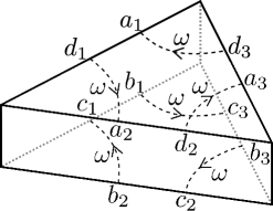
Figure 12: Triangles with the color structure. $\omega$ has the value $\omega^{da}$ when it is inserted into the index line from $d$ to $a$. Note that $\omega^{bc}=(\omega^{-1})^{cb}$.

Note that only $\omega$ (not $\omega^{-1}$) are accumulated when following the arrows in each index line. Thus, the value of a closed index loop forming $\ell$-gon changes from $\mathrm{tr}\,1_{n}=n=3m$ to

$$\mathrm{tr}(\omega^{\ell})=\left\{\begin{array}[]{l}n\phantom{0}\hskip 10.00002pt(\ell=0\mod 3)\\ 0\phantom{n}\hskip 10.00002pt(\ell\neq 0\mod 3).\end{array}\right.$$ (3.18)

We thus see that the index function of a diagram gives a nonvanishing value only when the index network around every vertex has a polygonal decomposition where the number of segments of each polygon is a multiple of three.

Note that such polygonal decompositions with nonvanishing index functions have the following dependence on the coupling constants. Suppose that the index network around vertex $v$ has $t_{2}(v)$ polygons, $t_{1}(v)$ segments and $t_{0}(v)$ junctions. Here, $t_{2}(v)=\sum_{\ell}t^{\ell}_{2}(v)$ with $t^{\ell}_{2}(v)$ the number of $\ell$-gons, and $t_{0}(v)=\sum_{k}t^{k}_{0}(v)$ with $t_{0}^{k}(v)$ the number of $k$-junctions. It is easy to see that the function $d(v)\equiv 2t_{1}(v)-3t_{2}(v)$ can be expressed as $d(v)=\sum_{\ell}(\ell-3)\,t^{\ell}_{2}(v)$. Thus $d(v)$ is nonnegative for the $C$’s in (3.14) because monogons and digons are excluded due to the color structure [i.e., $t^{\ell=1}_{2}(v)=t^{\ell=2}_{2}(v)=0$]. Recalling that the contribution from each diagram is given by

$$\frac{1}{S}\,\lambda^{s_{2}}\,\Bigl{(}\,\prod_{k\geq 2}\mu_{k}^{s_{1}^{k}}\Bigr{)}\prod_{v:\,\text{vertex}}n^{2-2g(v)},$$ (3.19)

and noting that the identification rule of the polygonal decompositions gives the relations

$$s_{2}=\frac{1}{3}\sum_{v}t_{1}(v),\quad s_{1}^{k}=\frac{1}{2}\sum_{v}t_{0}^{k}(v),$$ (3.20)

we find another expression of (3.19):

$$\frac{1}{S}\,\lambda^{s_{2}}\,\Bigl{(}\,\prod_{k\geq 2}\mu_{k}^{s_{1}^{k}}\Bigr{)}\prod_{v:\,\text{vertex}}n^{2-2g(v)}=\frac{1}{S}\,\prod_{v:\,\text{vertex}}\biggl{[}\Bigl{[}\,\prod_{k\geq 2}(\lambda^{2}\mu_{k})^{\frac{1}{2}t_{0}^{k}(v)}\Bigr{]}\Bigl{(}\frac{n}{\lambda}\Bigr{)}^{2-2g(v)}\Bigl{(}\frac{1}{\lambda}\Bigr{)}^{\frac{1}{3}d(v)}\biggr{]}.$$ (3.21)

Therefore, if we expand the free energy around $\lambda=\infty$ with $\lambda^{2}\,\mu_{k}$ and $n/\lambda$ being fixed, the leading contribution comes from such diagrams that satisfy $d(v)=0$ for every vertex $v$, namely, from the diagrams where every index network forms a triangular decomposition.

3.3 Counting the number of vertices

One may think from (3.21) that it would be possible by taking a limit $n/\lambda\to\infty$ to single out the diagrams where the index networks are all homeomorphic to two-sphere $S^{2}$. However, this is not the case. For example, let us consider a diagram which includes an index network forming a two-torus $T^{2}$. Since the index network gives the contribution of $(n/\lambda)^{0}=1$, we cannot distinguish a diagram whose vertices all give index networks homeomorphic to $S^{2}$ from a diagram which has the same number of such vertices whose index networks are homeomorphic to $S^{2}$ but also has extra vertices whose index networks are homeomorphic to $T^{2}$, because the contributions from the two diagrams to the free energy have the same form.

This problem comes from the fact that we cannot control the number of vertices only with the coupling constants existing in the model with $\mathcal{A}=M_{n}(\mathbb{R})$. However, this can be remedied by setting the algebra $\mathcal{A}$ to be the direct sum of $K$ copies of matrix ring $\mathcal{A}_{0}=M_{n}(\mathbb{R})$,

$$\mathcal{A}=\underbrace{\mathcal{A}_{0}\oplus\cdots\oplus\mathcal{A}_{0}}_{K~{}{\rm copies}}=K\mathcal{A}_{0}.$$ (3.22)

In fact, the index function of a diagram with $s_{0}$ vertices becomes proportional to $K^{s_{0}}$ since the index network around each vertex gives a factor of $K$ independently, and thus (3.21) changes to

$$\frac{1}{S}\,\prod_{v:\,\text{vertex}}\biggl{[}K\Bigl{[}\prod_{k\geq 2}(\lambda^{2}\mu_{k})^{\frac{1}{2}t_{0}^{k}(v)}\Bigr{]}\Bigl{(}\frac{n}{\lambda}\Bigr{)}^{2-2g(v)}\Bigl{(}\frac{1}{\lambda}\Bigr{)}^{\frac{1}{3}d(v)}\biggr{]}.$$ (3.23)

Therefore, we can single out the diagrams where every index network is homeomorphic to $S^{2}$, by picking out only the diagrams whose index function gives the values with the same power of $K$ as that of $n^{2}$.

3.4 Reduction to manifolds

Combining the results in subsections 3.2 and 3.3, we can reduce the set of possible diagrams to those whose index networks all give triangular decompositions of two-sphere $S^{2}$. We then can apply the following theorem to conclude that these diagrams represent tetrahedral decompositions of three-dimensional manifolds:

Theorem. Assume that the index network around every vertex in diagram $\gamma$ gives a triangular decomposition of two-sphere. Then, $\gamma$ represents a tetrahedral decomposition of a three-dimensional manifold.

Proof.

We label the vertices, triangles and hinges of diagram $\gamma$ as $v$ $(=1,2,3,\ldots)$, $f$ $(=i,j,k,\ldots)$ and $h$ $(=A,B,C,\ldots)$, respectively. Let $\mathcal{T}_{v}$ denote the index network around vertex $v$, which we assume to have a form of triangular decomposition of two-sphere. Note that every corner of a triangle in $\gamma$ corresponds to a segment of the index network around some vertex (see Fig. 13).

Figure 13: A part of diagram $\gamma$. The triangle $(i_{1},j_{1},k_{1})$ is a part of the index network around vertex 1, which has a form of triangular decomposition.

We denote by $f_{v}$ the segment which is lying on triangle $f$ and is placed in the corner at vertex $v$.

We choose a vertex (say $v=1$) and focus on an “index triangle” formed by three segments $i_{1},j_{1},k_{1}$ in $\mathcal{T}_{1}$. Here, $i,j,k$ are the triangles on which the three segments live. Since all the edges of each triangle are attached to hinges, there are hinges $A=(12)$, $B=(13)$, $C=(14)$, $D=(34)$, $E=(42)$, $F=(23)$ as in Fig. 13. As is depicted there, the three index triangles $(i_{2},k_{2},l_{2})$, $(i_{3},j_{3},l^{\prime}_{3})$ and $(j_{4},k_{4},l^{\prime\prime}_{4})$ ensure the existence of the corresponding triangles $l$, $l^{\prime}$ and $l^{\prime\prime}$, respectively. We are now going to give a detailed description of these triangles and show that they all coincide, $l=l^{\prime}=l^{\prime\prime}$.

We first take a look at hinge $A=(12)$. We assume that $2\to 1$ is the positive direction of hinge $A$ and label the triangles such that triangle $k$ is to the immediate left of $i$ when seen from vertex 1 (see Fig. 13). This means that triangle $k$ is to the immediate right of $i$ when seen from vertex 2, so that $i_{2}$ and $k_{2}$ are two segments of an index triangle around vertex 2, which will be complemented by the third segment $l_{2}$ as in Fig. 13. The triangle $l$ on which the segment $l_{2}$ lives is glued to triangle $i$ along hinge $F=(23)$, and must be to the immediate left of $i$ when seen from vertex 2 in the direction of $F$.

We repeat the same argument for hinge $B=(13)$. There, triangle $j$ is to the immediate right of $i$ when seen from vertex 1. This means that triangle $j$ is to the immediate left of $i$ when seen from vertex 3, so that $i_{3}$ and $j_{3}$ are two segments of an index triangle around vertex 3, which will be complemented by the third segment $l^{\prime}_{3}$ as in Fig. 13. The triangle $l^{\prime}$ on which the segment $l^{\prime}_{3}$ lives is glued to triangle $i$ along hinge $F=(23)$, and must be to the immediate right of $i$ when seen from vertex 3 in the direction of $F$. However, this means that $l^{\prime}$ is to the immediate left of $i$ when seen from vertex 2, and thus two triangles $l$ and $l^{\prime}$ must be the same.

The same argument can also be made for hinge $C=(14)$, and we obtain $l=l^{\prime}=l^{\prime\prime}$, from which we see that there exists a tetrahedron surrounded by four triangles $i$, $j$, $k$, $l$. By repeating the same arguments for all the index triangles around every vertex, we conclude that diagram $\gamma$ gives a tetrahedral decomposition. Furthermore, since the index network around every vertex represents a triangular decomposition of $S^{2}$, the neighborhood of every vertex is homeomorphic to $B^{3}$. Therefore, the diagram $\gamma$ gives a tetrahedral decomposition of a three-dimensional manifold. ∎

3.5 Three-dimensional gravity

We have shown that a class of our models allow us to single out the diagrams which represent tetrahedral decompositions of three-dimensional manifolds. Such models can be used to define discretized three-dimensional Euclidean gravity. In fact, we only need to follow the arguments given in [34, 20, 21].

The action of three-dimensional Euclidean gravity is given by

$$S_{0}=-\kappa_{0}\int\!d^{3}x\sqrt{g}\,R+\Lambda_{0}\int\!d^{3}x\sqrt{g},$$ (3.24)

where $\kappa_{0}$ corresponds to the bare gravitational coupling and $\Lambda_{0}$ to the bare cosmological constant. This can be discretized by using regular tetrahedra with fixed spacing $a$ as

$$S_{\mathrm{EH}}=-4\pi\kappa_{0}a\,s_{0}\,+\Bigl{[}\frac{\sqrt{2}a^{3}}{12}\Lambda_{0}-4\pi\kappa_{0}a\Bigl{(}1-\frac{3\theta}{\pi}\Bigr{)}\Bigr{]}s_{3}.$$ (3.25)

Here, $s_{0}$ and $s_{3}$ denote the number of vertices and tetrahedra, respectively, and $\theta\equiv\arccos(1/3)$ is the angle between two neighboring triangles in a regular tetrahedron. The free energy of this action is then given by

$$\log Z_{\mathrm{EH}} =\sum_{\mathrm{config.}}\frac{1}{S}\,e^{-S_{\mathrm{EH}}}$$

$$=\sum_{\mathrm{config.}}\frac{1}{S}\,(e^{4\pi\kappa_{0}a})^{s_{0}}\,\bigl{(}e^{-\frac{\sqrt{2}a^{3}}{12}\Lambda_{0}+4\pi\kappa_{0}a\bigl{(}1-\frac{3\theta}{\pi}\bigr{)}}\bigr{)}^{s_{3}},$$ (3.26)

where $S$ is the symmetry factor.

In our models, on the other hand, each diagram representing a tetrahedral decomposition contributes to the free energy as

$$\frac{1}{S}\,\lambda^{s_{2}}\mu^{s_{1}}N^{s_{0}},$$ (3.27)

Here we have set $\mu_{k}\equiv\mu$ $(\forall k\geq 2)$. Since the relations $s_{2}=2s_{3}$ and $s_{1}=s_{0}+s_{3}$ hold for tetrahedral decompositions of a three-dimensional manifold, the contribution takes the form

$$\frac{1}{S}\,(\mu N)^{s_{0}}(\lambda^{2}\mu)^{s_{3}}.$$ (3.28)

Comparing (3.26) and (3.28), we obtain the relations between the coupling constants of the two models,

$$\mu N=e^{4\pi\kappa_{0}a},\qquad\lambda^{2}\mu=e^{-\frac{\sqrt{2}a^{3}}{12}\Lambda_{0}+4\pi\kappa_{0}a\bigl{(}1-\frac{3\theta}{\pi}\bigr{)}}.$$ (3.29)

3.6 Duality

We conclude this section by commenting that there exists a novel strong-weak duality which interchanges the roles of triangles and hinges when $\mathcal{A}$ is a matrix ring. We expect this duality to play an important role when we further study the analytic properties of the models in the future.

We first recall that one has two choices when introducing a structure of associative algebra to the tensor product of linear spaces, $\mathcal{R}=\mathcal{A}\otimes\bar{\mathcal{A}}$ [see (2.10)]. The first is the algebra structure as the tensor product of two associative algebras $\mathcal{A}$ and $\bar{\mathcal{A}}$. This is the structure we have used exclusively so far, and gives the multiplication (2.15) (denoted by $\times$), which can also be written as

$$(B_{1}\times B_{2})^{ij}\equiv(B_{1}\times B_{2})^{i}_{\phantom{i}k}\,\sigma^{kj}=B_{1}^{kl}B_{2}^{mn}y_{km}^{\phantom{km}i}y_{nl}^{\phantom{nl}j}\quad\text{for}~{}~{}B_{1},B_{2}\in\mathcal{R}.$$ (3.30)

The second is the algebra structure as the set of endomorphisms of $\mathcal{A}$ ; $\mathcal{R}={\rm End}\,\mathcal{A}$. The multiplication is defined as the composition of two linear operators acting on $\mathcal{A}$ and will be denoted by dot “$\,\cdot\,$”:

$$B_{1}\cdot B_{2}=(B_{1}\cdot B_{2})^{i}_{\phantom{i}j}e_{i}\otimes\bar{e}^{j}\equiv(B_{1})^{i}_{\phantom{i}k}(B_{2})^{k}_{\phantom{k}j}e_{i}\otimes\bar{e}^{j}\quad\text{for}~{}~{}B_{1},B_{2}\in\mathcal{R},$$ (3.31)

which can also be written as

$$(B_{1}\cdot B_{2})^{ij}\equiv(B_{1}\cdot B_{2})^{i}_{\phantom{i}k}\,\sigma^{kj}=B_{1}^{ik}\sigma_{kl}B_{2}^{lj}.$$ (3.32)

We will show that there is a duality between the two algebra structures when $\mathcal{A}$ is a matrix ring.

We first set $\sigma_{ij}=g_{ij}$. This is possible because $\sigma$ can be chosen in an arbitrary way [see a comment following (2.25)]. Then, when $\mathcal{A}=M_{n}(\mathbb{R})$, the multiplications are represented as

$$(B_{1}\times B_{2})^{abcd} =B_{1}^{aefd}B_{2}^{ebcf},$$ (3.33)

$$(B_{1}\cdot B_{2})^{abcd} =B_{1}^{abef}g_{efgh}B_{2}^{ghcd}=n\,B_{1}^{abef}B_{2}^{fecd}.$$ (3.34)

We now introduce the dual variables $\tilde{B}$ to $B$ as

$$\tilde{B}^{abcd}\equiv B^{bcda},$$ (3.35)

which satisfy the symmetry property $\tilde{B}^{abcd}=\tilde{B}^{cdab}$ due to (3.5). Then one can easily show from (3.33) and (3.34) that the two multiplications are interchanged for the dual variables:

$$(B_{1}\times B_{2})^{abcd}=\frac{1}{n}(\tilde{B}_{2}\cdot\tilde{B}_{1})^{bcda},\qquad(B_{1}\cdot B_{2})^{abcd}=n(\tilde{B}_{1}\times\tilde{B}_{2})^{bcda}.$$ (3.36)

We further introduce the variables $\tilde{A}$ dual to $A$ as

$$\tilde{A}_{abcd}\equiv A_{bcda}\,\bigl{(}=\tilde{A}_{cdab}\bigr{)}.$$ (3.37)

Then the action (3.4) can be rewritten in terms of the dual variables $\tilde{A}$ and $\tilde{B}$ to the form

$$S=\frac{1}{2}\tilde{A}_{abcd}\tilde{B}^{abcd}-\frac{\lambda}{6n^{3}}\tilde{A}_{abcd}\tilde{A}_{befc}\tilde{A}_{eadf}-\sum_{k\geq 2}\frac{n^{2}\mu_{k}}{2k}\tilde{B}^{a_{1}b_{1}b_{2}a_{2}}\tilde{B}^{a_{2}b_{2}b_{3}a_{3}}\ldots\tilde{B}^{a_{k}b_{k}b_{1}a_{1}}.$$ (3.38)

Note that the way to contract the indices of $\tilde{A}$ (or $\tilde{B}$) in the dual action (3.38) is the same as that of $B$ (or $A$) in the original action (3.4). This means that a triangle for the original variables, (3.11), now plays the role of a 3-hinge for the dual variables, and a $k$-hinge for the original variables, (3.13), plays the role of a $k$-gon for the dual variables. We thus find that the action (3.38) for the dual variables generates the dual diagrams to the original ones, consisting of $3$-hinges (dual to original triangles) and polygons (dual to original hinges). Note that the large $N$ limit in (3.21) ($n\to\infty$ with $\lambda^{2}\mu_{k}$ and $n/\lambda$ being fixed) gives $\lambda\to\infty$ and $\mu_{k}=\mu\to 0$. Since $\lambda$ and $\mu$ are interchanged in the duality transformation, one sees that this duality is actually a strong-weak duality.

4 Group ring

In this section, we investigate the models where $\mathcal{A}$ is set to be a group ring $\mathbb{R}[G]$, and demonstrate how the models depend on details of the group structure of $G$. We assume that $G$ is a finite group with order $|G|$ in order to avoid introducing regularizations, although most of the relations below can be applied to continuous compact groups.

4.1 Action for a group ring

Group ring $\mathbb{R}[G]$ is an associative algebra linearly spanned by the elements of $G$, $\mathbb{R}[G]=\bigoplus_{x\in G}\mathbb{R}e_{x}$, with multiplication rule determined by that of group $G$,

$$e_{x}\times e_{y}=e_{xy}.$$ (4.1)

The structure constants $y_{x,y}^{\phantom{x,y}z}$ are then given by

$$y_{x,y}^{\phantom{x,y}z}=\delta(xy,z).$$ (4.2)

Here, the contraction of repeated indices is understood to represent the integration with the normalized Haar measure $\int dx\equiv\frac{1}{|G|}\sum_{x}$:

$$y_{x,y}^{\phantom{x,y}z}e_{z}\equiv\int\!dz\,y_{x,y}^{\phantom{x,y}z}e_{z}=\frac{1}{|G|}\sum_{z}y_{x,y}^{\phantom{x,y}z}e_{z},$$ (4.3)

and $\delta(x,y)$ is the delta function with respect to this measure:

$$\delta(x,y)\equiv|G|\,\delta_{x,y},\qquad\int\!dx\,f(x)\,\delta(x,y)=f(y).$$ (4.4)

From the definition we obtain

$$y_{x_{1},x_{2},\ldots,x_{k}} =\delta(x_{1}x_{2}\cdots x_{k},1),$$ (4.5)

$$g^{x,y} =\delta(xy,1),$$ (4.6)

where $1$ is the identity of $G$. Therefore, the action (2.25) can be written with the symmetric dynamical variables $A_{x,y}=A_{y,x}$ and $B^{x,y}=B^{y,x}$ as

$$S[A,B] =\frac{1}{2}A_{x,y}\,B^{x,y}-\frac{\lambda}{6}A_{x^{-1},y}\,A_{y^{-1},z}\,A_{z^{-1},x}$$

$$~{}~{}~{}-\sum_{k\geq 2}\frac{\mu_{k}}{2k}\,B^{x_{1}y_{1}}\cdots B^{x_{k}y_{k}}\,\delta(x_{1}\cdots x_{k},1)\,\delta(y_{k}\cdots y_{1},1).$$ (4.7)

4.2 The Feynman rules and the free energy for a group ring

The action (4.7) can be rewritten to a form similar to that of matrix ring, by expressing everything in terms of the irreducible representations of $G$. To show this, we first write the delta function as

$$\delta(x_{1}\cdots x_{k},1)=\sum_{R}d_{R}\,\mathrm{tr}(D_{R}(x_{1})\cdots D_{R}(x_{k})),$$ (4.8)

where the sum is taken over all the irreducible representations $R$ of $G$ with the representation matrix $D_{R}(x)=(D^{R}_{ab}(x))$ $(x\in G)$, and $d_{R}$ is the dimension of representation $R$, $d_{R}=\mathrm{tr}\,D_{R}(1)$. Then, the action (4.7) can be rewritten to the form

$$S =\frac{1}{2}\sum_{R,S}d_{R}\,d_{S}A^{RS}_{abcd}B^{RS}_{abcd}-\frac{\lambda}{6}\sum_{R_{1},R_{2},R_{3}}d_{R_{1}}d_{R_{2}}d_{R_{3}}A^{R_{1}R_{2}}_{a_{1}b_{1}b_{2}a_{2}}A^{R_{2}R_{3}}_{a_{2}b_{2}b_{3}a_{3}}A^{R_{3}R_{1}}_{a_{3}b_{3}b_{1}a_{1}}$$

$$\quad-\sum_{k\geq 2}\frac{\mu_{k}}{2k}\sum_{R,S}d_{R}\,d_{S}\,B^{RS}_{a_{1}a_{2}b_{2}b_{1}}\cdots B^{RS}_{a_{k}a_{1}b_{1}b_{k}},$$ (4.9)

where

$$A^{RS}_{abcd} \equiv\int\!dxdy\,A_{x,y}D^{R}_{ab}(x)D^{S}_{cd}(y)=A^{SR}_{cdab},$$ (4.10)

$$B^{RS}_{abcd} \equiv\int\!dxdy\,B^{x,y}D^{R}_{ba}(x^{-1})D^{S}_{dc}(y^{-1})=B^{SR}_{cdab}.$$ (4.11)

This action gives the following Feynman rules:

$${\rm propagator} :\ \begin{array}[]{l}\includegraphics[height=42.67912pt]{fig4-01.eps}\end{array}+\begin{array}[]{l}\includegraphics[height=42.67912pt]{fig4-02.eps}\end{array}$$ (4.14)

$$\quad\sim\langle A^{RS}_{abcd}B^{R^{\prime}S^{\prime}}_{efgh}\rangle=\frac{1}{d_{R}d_{S}}(\delta_{ae}\delta_{bf}\delta_{cg}\delta_{dh}\delta^{RR^{\prime}}\delta^{SS^{\prime}}+\delta_{ag}\delta_{bh}\delta_{ce}\delta_{df}\delta^{RS^{\prime}}\delta^{SR^{\prime}}),$$ (4.15)

$${\rm triangle} :\ \begin{array}[]{l}\includegraphics[width=113.81102pt]{fig4-03.eps}\end{array}\sim\lambda\,d_{R_{1}}d_{R_{2}}d_{R_{3}}\delta_{a_{1}d_{2}}\delta_{c_{1}b_{2}}\ldots\delta_{a_{k}d_{1}}\delta_{c_{k}d_{1}},$$ (4.17)

$$k :\ \begin{array}[]{l}\includegraphics[width=85.35826pt]{fig4-04.eps}\end{array}\sim\mu_{k}\,d_{R}\,d_{S}\,\delta_{a_{1}b_{2}}\delta_{d_{1}c_{2}}\ldots\delta_{a_{k}b_{1}}\delta_{d_{k}c_{1}}.$$-hinge (4.19)

We thus see that the index network around every vertex is again expressed as a closed surface with double index lines, and its index function is determined only by the Euler characteristics of the polygonal decomposition:

$$\mathcal{F}(\gamma)=\prod_{v:\,\text{vertex}}\mathcal{I}_{g(v)}=\prod_{v:\,\text{vertex}}\Bigl{[}\sum_{R}(d_{R})^{2-2g(v)}\Bigr{]}.$$ (4.20)

Here, elementary group theory shows that $\sum_{R}d_{R}^{2}=|G|$, and $\sum_{R}d_{R}^{0}$ gives the number of irreducible representations which equals that of conjugate classes. For example, when $G$ is the symmetric group $S_{n}$, we have

$$\sum_{R}d_{R}^{2}=|G|=n!\,,\qquad\sum_{R}d_{R}^{0}=p_{n},$$ (4.21)

where $p_{n}$ denotes the number of partitions of $n$. Therefore, if $G$ admits the relations $\sum_{R}d_{R}^{2}\gg\sum_{R}d_{R}^{2-2g}$ $(g\geq 1)$, the index networks of spherical topology have a large value of index function compared to those of higher genera.

We also can introduce a color structure as in subsection 3.2 and can control the number of vertices by considering the direct sum of $K$ copies of group ring as in subsection 3.3. Therefore, we can again single out the diagrams which give tetrahedral decompositions of three-dimensional manifolds.

5 Summary and discussion

In this paper we construct a class of models that generate random diagrams consisting of triangles and multiple hinges. The models are completely characterized by semisimple associative algebras $\mathcal{A}$ and tensors $C^{ijklmn}$. When $C^{ijklmn}$ are chosen as in (2.26) or (3.14), each Feynman diagram can be expressed as a collection of index networks around vertices. The contribution $\mathcal{F}(\gamma)$ from each diagram $\gamma$ to the free energy is expressed as the product of the index functions $\zeta(v)$ of vertices $v$ of $\gamma$, and $\zeta(v)$ depends only on the topology of the index network around $v$ besides the structure of the defining associative algebra.

Although most of the Feynman diagrams do not represent three-dimensional manifolds, we give a general prescription to automatically reduce the set of possible diagrams such that only (and all of the) manifolds are generated. We implement the strategy for the models with $\mathcal{A}$ set to matrix rings, by introducing a color structure and taking the direct sum of $K$ copies of matrix ring. We show that every diagram actually gives a tetrahedral decomposition where each vertex has a neighborhood homeomorphic to $B^{3}$ (ensured by the statement that the index network around each vertex has the topology of $S^{2}$).

We further demonstrate that there is a novel strong-weak duality in the models which interchanges the roles of triangles and hinges. We also investigate the models where the defining associative algebras are group rings, and show that most of their analytic properties can be understood as a straightforward generalization of those for matrix rings.

We now list some of the future directions for further study of the models. The first is about the topology summation. Our models actually give a summation over all topologies of three-dimensional manifolds. It seems that we cannot distinguish the topology of the Feynman diagrams if the tensor $C^{ijklmn}$ has the form (2.26) or (3.14) as we took in this paper, because topologically different diagrams can give contributions of the same form to the free energy. One can optimistically think that this represents membrane instability (see, e.g., [3]). However, it may also happen that configurations of some specific topology entropically dominate in a critical region, although we have not fully evaluated the numerical coefficients in the free energy and their dependence on topology.

Another way to investigate the topologies of diagrams is to change the tensor $C^{ijklmn}$ to other forms. In fact, this change significantly modifies the dependence of the index function on the associative algebra $\mathcal{A}$. The change of $C^{ijklmn}$ and its effect on topological invariants will be studied in our future paper [35].

The second direction for further study is about the continuum limit. Although we have not fully studied the continuum limit yet, there may be a chance to analytically solve the models in the large $N$ limit and to determine the critical behaviors, because the dynamical variables of our models are given by symmetric matrices $A_{ij}$ and $B^{ij}$.

The third direction is about the introduction of matters to our models. We expect that extra degrees of freedom representing matter fields can be introduced by making copies of the variables $A_{ij}$ and $B^{ij}$ as in matrix models [9]. It should be particularly interesting to introduce matter fields corresponding to the target space coordinates of embedded membranes and to study the critical behaviors. It would then be important to investigate if there is an analogue of the so-called “$c=1$ barrier” in the models and how the situation is modified when supersymmetry is introduced.

We close this section with a brief comment on the relationship of our models with the colored tensor models. It is worth noting that our models (with a color structure and an appropriate limit of parameters as in subsection 3.4) generate all  of the possible tetrahedral decompositions of three-dimensional manifolds, and thus should have more configurations than those of the colored tensor models. For example, the colored tensor models do not generate such tetrahedral decompositions where odd number of triangles are glued together along a hinge. Since the colored tensor models introduce a pair of tensors as in two-matrix models, they may correspond to three-dimensional gravity with specific matters. In this sense, our models with minimum fine tunings may give a continuum theory (if exists) closer to pure gravity. It should be interesting to investigate whether colored tensor models can be obtained by adding some (not necessarily unitary) matters to our models.

In a remarkable paper [27], it is shown that the free energy of three-dimensional colored tensor models depend on the size of tensor, $\mathcal{N}$, as

$$\mathcal{N}^{3}\sum_{\mathcal{G}}\mathcal{N}^{-\omega(\mathcal{G})},$$ (5.1)

where we have suppressed other coupling constants. $\mathcal{G}$ denotes a colored graph which is dual to a tetrahedral decomposition of three-dimensional pseudomanifold, and $\omega(\mathcal{G})$ is the degree of $\mathcal{G}$ (see [27] for details). Thus, in the large $\mathcal{N}$ limit, the leading contribution comes from colored graphs with $\omega(\mathcal{G})=0$. It is also shown that if $\omega(\mathcal{G})=0$ then $\mathcal{G}$ is dual to a three-sphere [26]. Therefore, the leading order graphs are homeomorphic to $S^{3}$. We can say the same thing for our models if we confine our attention to only the diagrams that have tetrahedral decompositions dual to colored graphs. The degree $\omega$ of such a diagram can be evaluated as in [27] and becomes

$$\omega=\frac{3}{2}s_{3}+3-s_{1},$$ (5.2)

with which the contribution (3.28) to the free energy can be rewritten to the form

$$\frac{1}{S}\Bigl{(}\frac{N}{\lambda^{2}}\Bigr{)}^{-\frac{2}{3}\omega+2}\bigl{(}\lambda^{4}\mu^{3}N\bigr{)}^{\frac{1}{3}s_{1}}.$$ (5.3)

Thus, if we take a limit $N/\lambda^{2}\to\infty$ with $\lambda^{4}\mu^{3}N$ kept finite, the leading contribution comes from configurations with $\omega=0$, that is, tetrahedral decompositions of $S^{3}$. It is interesting to study the meaning of the degree for general tetrahedral decompositions which are not dual to colored graphs.

References

- [1] E. Witten, “String theory dynamics in various dimensions,” Nucl. Phys. B 443 (1995) 85 [hep-th/9503124].
- [2] T. Banks, W. Fischler, S. H. Shenker and L. Susskind, “M theory as a matrix model: A conjecture,” Phys. Rev. D 55 (1997) 5112 [hep-th/9610043].
- [3] W. Taylor, “M(atrix) theory: Matrix quantum mechanics as a fundamental theory,” Rev. Mod. Phys. 73 (2001) 419 [hep-th/0101126].
- [4] V. G. Knizhnik, A. M. Polyakov and A. B. Zamolodchikov, “Fractal structure of 2D quantum gravity,” Mod. Phys. Lett. A 3 (1988) 819.
- [5] F. David, “Conformal field theories coupled to 2D gravity in the conformal gauge,” Mod. Phys. Lett. A 3 (1988) 1651.
- [6] J. Distler and H. Kawai, “Conformal field theory and 2D quantum gravity Or Who’s Afraid of Joseph Liouville?,” Nucl. Phys. B 321 (1989) 509.
- [7] P. H. Ginsparg and G. W. Moore, “Lectures on 2-D gravity and 2-D string theory,” In Boulder 1992, Proceedings, Recent directions in particle theory, 277-469 [hep-th/9304011].
- [8] P. Di Francesco, P. H. Ginsparg and J. Zinn-Justin, “2-D Gravity and random matrices,” Phys. Rept. 254 (1995) 1 [hep-th/9306153].
- [9] V. A. Kazakov and A. A. Migdal, “Recent progress in the theory of noncritical strings,” Nucl. Phys. B 311 (1988) 171.
- [10] G. ’t Hooft, “A planar diagram theory for strong interactions,” Nucl. Phys. B 72 (1974) 461.
- [11] E. Brézin and V. A. Kazakov, “Exactly solvable field theories of closed strings,” Phys. Lett. B 236 (1990) 144.
- [12] M. R. Douglas and S. H. Shenker, “Strings in less than one dimension,” Nucl. Phys. B 335 (1990) 635.
- [13] D. J. Gross and A. A. Migdal, “Nonperturbative two-dimensional quantum gravity,” Phys. Rev. Lett. 64 (1990) 127.
- [14] M. Fukuma, H. Kawai and R. Nakayama, “Continuum Schwinger-Dyson equations and universal structures in two-dimensional quantum gravity,” Int. J. Mod. Phys. A 6 (1991) 1385.
- [15] R. Dijkgraaf, H. L. Verlinde and E. P. Verlinde, “Loop equations and Virasoro constraints in nonperturbative 2-D quantum gravity,” Nucl. Phys. B 348 (1991) 435.
- [16] S. H. Shenker, “The Strength of nonperturbative effects in string theory,” In “Cargèse 1990, Proceedings, Random surfaces and quantum gravity” 191–200.
- [17] M. R. Douglas, “Strings in less than one dimension and the generalized KdV hierarchies,” Phys. Lett. B 238 (1990) 176.
- [18] M. Fukuma, H. Kawai and R. Nakayama, “Infinite dimensional Grassmannian structure of two-dimensional quantum gravity,” Commun. Math. Phys. 143 (1992) 371.
- [19] M. Fukuma, H. Kawai and R. Nakayama, “Explicit solution for – duality in two-dimensional quantum gravity,” Commun. Math. Phys. 148 (1992) 101.
- [20] J. Ambjorn, B. Durhuus and T. Jonsson, “Three-dimensional simplicial quantum gravity and generalized matrix models,” Mod. Phys. Lett. A 6 (1991) 1133.
- [21] N. Sasakura, “Tensor model for gravity and orientability of manifold,” Mod. Phys. Lett. A 6 (1991) 2613.
- [22] M. Gross, “Tensor models and simplicial quantum gravity in 2-D,” Nucl. Phys. Proc. Suppl. 25A (1992) 144.
- [23] D. V. Boulatov, “A model of three-dimensional lattice gravity,” Mod. Phys. Lett. A 7 (1992) 1629 [hep-th/9202074].
- [24] L. Freidel, “Group field theory: An overview,” Int. J. Theor. Phys. 44 (2005) 1769 [hep-th/0505016].
- [25] R. Gurau and J. P. Ryan, “Colored tensor models - a review,” SIGMA 8 (2012) 020 [arXiv:1109.4812 [hep-th]].
- [26] R. Gurau, “The complete expansion of colored tensor models in arbitrary dimension,” Annales Henri Poincare 13 (2012) 399 [arXiv:1102.5759 [gr-qc]].
- [27] V. Bonzom, R. Gurau and V. Rivasseau, “Random tensor models in the large limit: Uncoloring the colored tensor models,” Phys. Rev. D 85 (2012) 084037 [arXiv:1202.3637 [hep-th]].
- [28] S. Dartois, R. Gurau and V. Rivasseau, “Double scaling in tensor models with a quartic interaction,” JHEP 1309 (2013) 088 [arXiv:1307.5281 [hep-th]].
- [29] V. Bonzom, R. Gurau, J. P. Ryan and A. Tanasa, “The double scaling limit of random tensor models,” JHEP 1409 (2014) 051 [arXiv:1404.7517 [hep-th]].
- [30] S. w. Chung, M. Fukuma and A. D. Shapere, “Structure of topological lattice field theories in three dimensions,” Int. J. Mod. Phys. A 9 (1994) 1305 [hep-th/9305080].
- [31] J. Ambjorn, B. Durhuus and T. Jonsson, “Quantum geometry. A statistical field theory approach,” Cambridge University Press, 1997.
- [32] M. Fukuma, S. Hosono and H. Kawai, “Lattice topological field theory in two dimensions,” Commun. Math. Phys. 161 (1994) 157 [hep-th/9212154].
- [33] C. Bachas and P. M. S. Petropoulos, “Topological models on the lattice and a remark on string theory cloning,” Commun. Math. Phys. 152 (1993) 191 [hep-th/9205031].
- [34] D. Weingarten, “Euclidean quantum gravity on a lattice,” Nucl. Phys. B 210 (1982) 229.
- [35] M. Fukuma, S. Sugishita and N. Umeda, work in progress.