Separable projection integrals for higher-order correlators of the cosmic microwave sky: Acceleration by factors exceeding 100

Abstract

We present a case study describing efforts to optimise and modernise “Modal”, the simulation and analysis pipeline used by the Planck satellite experiment for constraining general non-Gaussian models of the early universe via the bispectrum (or three-point correlator) of the cosmic microwave background radiation. We focus on one particular element of the code: the projection of bispectra from the end of inflation to the spherical shell at decoupling, which defines the CMB we observe today. This code involves a three-dimensional inner product between two functions, one of which requires an integral, on a non-rectangular domain containing a sparse grid. We show that by employing separable methods this calculation can be reduced to a one-dimensional summation plus two integrations, reducing the overall dimensionality from four to three. The introduction of separable functions also solves the issue of the non-rectangular sparse grid. This separable method can become unstable in certain scenarios and so the slower non-separable integral must be calculated instead. We present a discussion of the optimisation of both approaches.

We demonstrate significant speed-ups of $\approx$100$\times\mbox{ }$, arising from a combination of algorithmic improvements and architecture-aware optimisations targeted at improving thread and vectorisation behaviour. The resulting MPI/OpenMP hybrid code is capable of executing on clusters containing processors and/or coprocessors, with strong-scaling efficiency of 98.6% on up to 16 nodes. We find that a single coprocessor outperforms two processor sockets by a factor of 1.3$\times\mbox{ }$and that running the same code across a combination of both microarchitectures improves performance-per-node by a factor of 3.38$\times\mbox{ }$. By making bispectrum calculations competitive with those for the power spectrum (or two-point correlator) we are now able to consider joint analysis for cosmological science exploitation of new data.

1 Introduction

The current best explanation for the origin of our universe is the inflationary big bang scenario, where it is believed that a period of exponential expansion created the large flat empty universe we see today. In addition, this model predicts that quantum fluctuations in the energy during this time will be stretched to galactic scales forming the seeds from which all structure grew, from planets and stars through to super-clusters of galaxies. The statistics of these fluctuations give a window onto the dynamics at play during the birth of our universe. In particular, any deviation of these fluctuations from a Gaussian (i.e. Normal) distribution would be direct evidence of interesting new physics.

There has been enormous effort within the community to measure any possible deviations from Gaussianity with the bispectrum, the Fourier transform of the three point correlator, being the favoured statistic. The primary obstacle to naïve estimation of the bispectrum is that for the CMB it is 5 dimensional and would require $\mathcal{O}(10^{22})$ floating point operations to calculate, which is challenging for the world’s largest supercomputers. This can be overcome by using separable approximations for the bispectra, however the projection of the primordial bispectra forward to the time of observation remains a major obstacle to measurement. There are a multitude of approaches to this which divide into two main categories: ones that require non-Gaussian simulations to train estimators, [1, 2, 3, 4, 5, 6]; and those that use specific simple primordial templates for which projection is tractable, [7, 8, 9, 10].

The Modal method [11, 12] developed at the University of Cambridge, which is the focus of this paper, and used by the Planck satellite experiment [13, 14] is the only general method for constraining these non-Gaussianities from the available data. Its main strength is that by using a general mode expansion it can reduce the evolution from primordial to late times into a matrix projection, allowing us to constrain thousands of theoretical predictions simultaneously. By using an appropriate basis tuned for the theoretical models of interest, the Modal team have created a fast and efficient way to probe cosmological data for hints of new physics in the early universe.

This paper investigates the optimisation and modernisation of Modal, as part of an effort to accelerate it using Intel^® Xeon Phi^™ coprocessors. The existing MPI-level parallelism in the original code is not sufficient to enable efficient utilisation of this hardware, and we show that moving to a hybrid MPI/OpenMP implementation can significantly improve performance. For portability reasons, we avoid making any significant code changes that would benefit only one particular hardware platform, and thus the high-level programming languages and techniques that we use apply equally well to Intel^® Xeon^® processors. When compared to the original code on 2$\times\mbox{ }$processor sockets, our code optimisation efforts deliver speed-ups of 1765$\times\mbox{ }$on a single coprocessor and 833$\times\mbox{ }$on 2$\times\mbox{ }$processor sockets in the 2D case; and 108$\times\mbox{ }$on a coprocessor and 83.9$\times\mbox{ }$on 2$\times\mbox{ }$processor sockets in the 3D case. These speed-ups are large enough to significantly impact the rate of scientific discovery at COSMOS, and enable liberal use of the Modal calculation as part of future Monte Carlo pipelines – something that had previously been considered infeasible.

A number of previous studies have investigated the use of Intel Xeon Phi coprocessors to accelerate other scientific codes [15, 16, 17, 18, 19], and there are many similarities between the optimisations we discuss here and those explored in other domains. However, we note that many of these studies were performed before the standardisation of OpenMP 4.0 (and thus often rely on manual vectorisation via architecture-specific intrinsics). This is also the first paper (to the best of our knowledge) to explore the use of Intel Xeon Phi coprocessors for this specific application domain.

The rest of this paper is organized as follows: Section 2 provides an introduction to the two Modal routines which are being optimised – the full three dimensional calculation on the sparse non-rectangular domain, and the fast two dimensional version on a dense rectangular domain – and also provides a high-level introduction to Intel Xeon Phi coprocessors; Section 3 details the optimisation and modernisation of Modal; Section 4 presents a detailed performance study of the final application, demonstrating its scalability within a node and across multiple nodes; and finally, Section 5 concludes the paper, and discusses potential new uses for the accelerated version of the code.

2 Background

2.1 Direct Integration

The primary concern of this paper is the efficient calculation of a three-dimensional inner product which concerns the projection of a set of primordial basis bispectra defined at the end of inflation into a set of basis bispectra on a spherical shell defined by the CMB; that is, we evolve from an early-time basis into another different basis which is more convenient at late times. We consider two late-time bispectra $A_{\ell_{1}\ell_{2}\ell_{3}}$ and $B_{\ell_{1}\ell_{2}\ell_{3}}$ depending on the spherical harmonic multipoles $\ell_{i}$ and we take the following inner product betweeen them:

$$\left\langle A,\,B\right\rangle_{l} \equiv\sum_{\ell_{i}}\ \left(\frac{h_{\ell_{1}\ell_{2}\ell_{3}}}{v_{\ell_{1}}v_{\ell_{2}}v_{\ell_{3}}}\right)^{2}\,A_{\ell_{1}\ell_{2}\ell_{3}}\,B_{\ell_{1}\ell_{2}\ell_{3}}\,,$$ (1)

where the required weight function is:

$$h^{2}_{\ell_{1}\ell_{2}\ell_{3}}=\frac{(2\ell_{1}+1)(2\ell_{2}+1)(2\ell_{3}+1)}{4\pi}\left(\begin{array}[]{ccc}\ell_{1}&\ell_{2}&\ell_{3}\\ 0&0&0\end{array}\right)^{2}\,.$$ (4)

The array in brackets is the Wigner 3$J$ symbol, which is a geometric factor related to the projection onto the 2-sphere of the CMB. It has two important properties. Firstly, it is zero if the three $\ell_{i}$, when treated as lengths, are unable to form a triangle (the triangle condition) and secondly it is zero whenever $\ell_{1}+\ell_{2}+\ell_{3}$ is odd (the parity condition). These two conditions present complications in evaluating the sums over the $l_{i}$ as the region is non-rectangular and inside the allowed region all odd combinations must be excluded. These two constraints present issues with load balancing and vectorisation, which will be discussed later. When both these conditions are met, $h^{2}$ has an exact expression in terms of factorials which in turn can be accurately calculated using the Gosper approximation to the Wigner 3J symbol. The resulting expression is:

$$h^{2}_{\ell_{1}\ell_{2}\ell_{3}}\approx\frac{1}{2\pi^{2}}\frac{(2\ell_{1}+1)(2\ell_{2}+1)(2\ell_{3}+1)(L+1/3)}{(L+1)(L_{1}+1/3)(L_{2}+1/3)(L_{3}+1/3)}\sqrt{\frac{(L_{1}+1/6)(L_{2}+1/6)(L_{3}+1/6)}{(L+1/6)}}$$ (5)

where $L=\ell_{1}+\ell_{2}+\ell_{3}$ and $L_{i}=L-2\ell_{i}$. This inner product needs to be calculated between our projected primordial basis $\widetilde{Q}$, which unavoidably involves a radial integral along a line of sight from primordial times until now, and our late time basis $Q$. For the estimation and projection to be tractable we must form our basis functions from products of one-dimensional basis functions $\tilde{q}$ and $q$ respectively which must be symmetrised over the $\ell_{i}$. Writing it out explicitly in terms of these 1D functions:

$$\Gamma^{\prime}_{nn^{\prime}}=\left\langle Q_{n}\widetilde{Q}_{n^{\prime}}\right\rangle =\sum_{\ell_{1}=2}^{\ell_{max}}\sum_{\ell_{2}=2}^{\ell_{max}}\sum_{\ell_{3}=2}^{\ell_{max}}\frac{\theta_{\ell_{1}\ell_{2}\ell_{3}}}{72\pi^{2}}\frac{(2\ell_{1}+1)(2\ell_{2}+1)(2\ell_{3}+1)(L+1/3)}{(L+1)(L_{1}+1/3)(L_{2}+1/3)(L_{3}+1/3)v_{\ell_{1}}v_{\ell_{2}}v_{\ell_{3}}}$$

$$\times\sqrt{\frac{(L_{1}+1/6)(L_{2}+1/6)(L_{3}+1/6)}{(L+1/6)C_{\ell_{1}}C_{\ell_{2}}C_{\ell_{3}}}}\left(q_{i}(\ell_{1})q_{j}(\ell_{2})q_{k}(\ell_{3})+5\,\mbox{perms}\right)$$

$$\times\int r^{2}dr\left(\tilde{q}_{i^{\prime}}(r,\ell_{1})\tilde{q}_{j^{\prime}}(r,\ell_{2})\tilde{q}_{k^{\prime}}(r,\ell_{3})+5\,\mbox{perms}\right)$$ (6)

where $\theta$ is a top-hat like function (which is 1 when the triangle and parity conditions are met and 0 elsewhere) and there is a known mapping between $n\rightarrow ijk$. Evaluation of Equation 2.1 (where $v_{\ell}$, $C_{\ell}$ and $\tilde{q}$ have been precomputed) is performed by “Modal3D” (note that as we have a radial integral in addition to the three summations, the calculation is in fact four-dimensional for each of the $n_{max}^{2}$ independent matrix entries). For full details of the origin of Equation 2.1 see the Appendix. Typical values for the problem size are $n_{max}\approx 2000$, $\ell_{max}\approx 2000$ and approximately $200$ points needed to calculate the integral over $r$ using splines.

2.2 Separable Integration

One significant simplification that can be made in some cases is to note that the Wigner 3$J$ symbol can be written as an integral over three Legendre polynomials so $h^{2}$ in Equation 4 takes the exact form:

$$h^{2}_{\ell_{1}\ell_{2}\ell_{3}}=\frac{(2\ell_{1}+1)(2\ell_{2}+1)(2\ell_{3}+1)}{8\pi}\int d\mu P_{\ell_{1}}(\mu)P_{\ell_{2}}(\mu)P_{\ell_{3}}(\mu)\,.$$ (7)

This automatically preserves the triangle and parity conditions allowing us to work on a domain which is both rectangular and dense. This allows us to write Equation 2.1 in a much simpler form:

$$\Gamma^{\prime}_{nn^{\prime}} =\frac{1}{48\pi}\int r^{2}dr\int d\mu\left(P_{ii^{\prime}}(r,\mu)P_{jj^{\prime}}(r,\mu)P_{kk^{\prime}}(r,\mu)+5\,perms\right)\,,$$ (8)

where we have made the definition:

$$P_{ii^{\prime}}(r,\mu) \equiv\sum_{\ell}\frac{(2\ell+1)}{v_{\ell}\sqrt{C_{\ell}}}\tilde{q}_{i^{\prime}}(r,\ell)q_{i}(\ell)P_{\ell}(\mu)\,.$$ (9)

The simplified expression in Equation 8 is solved by “Modal2D”. One consequence of trying to retain the step like conditions of $h^{2}$ while using an integral form is that this calculation is very sensitive and must be done to very high precision. Fortunately as the integrand is polynomial we can use Gauss-Legendre quadrature which is, in principle, exact. However we found that standard libraries for calculation of weights and abscissas were not sufficiently accurate and we had to use a specialist implementation which had been optimised for this purpose [20] before the calculation proved stable for specific choices for $Q$ and $\bar{Q}$. We note that this stability is not sufficient to allow us to reverse the order of the $r$ and $\mu$ integrations and the $\mu$ integration must always be carried out first.

It is this issue with stability which leads us to retaining both implementations of the calculation. The 2D version is employed for any bispectra where bases can be chosen so that the integral representation of $h^{2}$ is stable, with any remaining cases being calculated by the slower but robust 3D version. We found that the majority of bispectra we are interested in can use the 2D version but there are some very well-motivated cases that cannot, for example the bispectrum induced by gravitational lensing.

The original code is written in C and parallelized with MPI. The 2D variant is parallelized over the loop of all the inner products $\left\langle Q_{n}\widetilde{Q}_{n^{\prime}}\right\rangle$, whereas the 3D variant is parallelized over the $n$ and $\ell_{1}$ indices in Equation 2.1. Throughout the rest of this paper, “Modal” without a 2D or 3D suffix can be assumed to refer to both variants of the application.

2.3 Intel Xeon Phi Coprocessors

An Intel Xeon Phi coprocessor consists of many ($\approx 60$) low frequency in-order cores which share a coherent memory. Each of these cores can run up to four hardware threads, which is useful for hiding the latencies of memory accesses and multi-cycle instructions in the absence of out-of-order execution. Unlike the “hyperthreads” on Intel Xeon processors, a single thread on the coprocesor cannot issue instructions on back-to-back cycles – it is therefore necessary to use at least two threads per core to fully utilize the hardware.

Each core additionally has support for 512-bit SIMD instructions from the Initial Many-core Instruction (IMCI) set. Executing a fully vectorized fused multiply add (FMA) every cycle amounts to 16 double precision FLOPs per cycle per core, or a theoretical peak of $\approx$1 TFLOP/s in double precision.

The coprocessor is physically mounted on a PCIe card with its own GDDR memory and Linux operating system. Since the cores are x86-based and run Linux, the coprocessor is amenable to existing parallel programming languages and libraries such as MPI and OpenMP – compiling existing codes for the coprocessor is often very simple, but extracting performance may require some significant algorithmic restructuring to expose sufficient parallelism [21].

2.4 Experimental Setup

Table 1: System configuration for a single node of Cosmic.

	Intel Xeon Processor E5-4650L	Intel Xeon Phi Coprocessor 5110P
Sockets$\times$Cores$\times$Threads	$1\times 8\times 1$	$1\times 60\times 4$
Clock (GHz)	2.6	1.053
Double Precision GFLOP/s	166.4	1010.88
L1 / L2 / L3 Cache (KB)	32 / 256 / 20,480	32 / 512 / -
DRAM (per node)	58 GB	8 GB GDDR
STREAM [22] Bandwidth	26.4 GB/s	165 GB/s
PCIe Bandwidth	6 GB/s
Compiler Version	icc v15.0.0.090
MPI Version	SGI MPT 2.10
MPSS Version	3.2.1

We use the Cosmic supercomputer at the University of Cambridge, which is an SGI UV2000 system consisting of 28 processors, 24 coprocessors, and 1.6 TB of RAM. The specification of a single node of Cosmic is given in Table 1. The host processors are based on the microarchitecture previously code-named “Sandy Bridge”, and the coprocessors on the microarchitecture previously code-named “Knights Corner”. For the sake of brevity, we refer to these two microarchitectures henceforth as “SNB” and “KNC”, respectively.

All experiments (unless otherwise stated) were performed using all of the cores available within a node, running the maximum number of threads supported – 4 threads on KNC and 1 thread on SNB (hyper-threading is disabled on the host) – and the thread affinity used on KNC is set using: KMP_AFFINITY=close,granularity=fine. KNC is used in offload mode, and no additional flags are passed to the compiler beyond those used for SNB: -O3 -xHost -mcmodel=medium -restrict -align -fno-alias -qopenmp. All experiments are repeated 5 times, and we present the average (mean), in order to account for system noise and any non-deterministic performance effects arising from threading.

Profiling and analysis of the code was performed using Intel^® VTune^™ Amplifier XE and the optimisation reporting functionality of the Intel^® C compiler. For both forms of the algorithm, we measure the performance in terms of the number of loop iterations executed by the whole code per second. Since the amount of work per loop iteration is different in the two cases, we differentiate between them by referring to them as 2D and 3D iterations per second (2D it/s and 3D it/s) respectively. Henceforth we will also adopt a convenient notation for displaying the performance figures for SNB and KNC side-by-side as a tuple – (SNB, KNC) it/s.

3 Optimisation and Modernisation

Prior to exploring any algorithmic changes, hardware-specific optimisations or code modernisations, we carried out some high-level refactoring of the two Modal variants to improve their performance. Specifically, we replaced a number of abstract “getter” functions used to retrieve array values from other compilation modules with inlined direct array accesses, removing function call overheads and providing the compiler with more optimisation freedom. Some occurrences of routines from the GNU Scientific Library (GSL) were also replaced with equivalent, pre-optimised, routines from the Intel^® Math Kernel Library (MKL).

The purpose of performing such a high-level refactoring before engaging in other optimisation activities is twofold: first, it ensures that the baseline performance of the code is representative of the performance of the original algorithm (as opposed to only its implementation); second, it exposes more accurately the incremental performance improvements from our subsequent changes to the code. After our refactoring, the SNB performance of the 3D variant of the algorithm increased by 3.27$\times\mbox{ }$, however the 2D variant showed negligible improvement.

3.1 Modal2D

The hotspot in the Modal2D code is in a function called gamma_pt (see Listing 1) which evaluates the inner-most integral over $\mu$ in Equation 10 via Gauss-Legendre (GL) quadrature, which we repeat here for clarity;

$$\Gamma^{\prime}_{nn^{\prime}} =\frac{1}{48\pi}\int r^{2}dr\int d\mu\left(P_{ii^{\prime}}(r,\mu)P_{jj^{\prime}}(r,\mu)P_{kk^{\prime}}(r,\mu)+5\,perms\right)$$ (10)

$$P_{ii^{\prime}}(r,\mu) \equiv\sum_{\ell}\frac{(2\ell+1)}{v_{\ell}\sqrt{C_{\ell}}}\tilde{q}_{i^{\prime}}(r,\ell)q_{i}(\ell)P_{\ell}(\mu)\,.$$ (11)

The indexes $mn$ are the element of $\Gamma^{\prime}$ being calculated with the index $i$ corresponding to the point in the $r$ integration. The $j$ loop is over the GL-quadrature points for $\mu$, $s$ cycles over $ijk$ and $r$ over $i^{\prime}j^{\prime}k^{\prime}$. The array Nmap is $P_{ii^{\prime}}$, with beta corresponding to $\tilde{q}$ and basis to $q$. The array factor contains the product of all functions solely of $\ell$ and the Legendre polynomial $P_{\ell}$. The $s1$-$6$ are the six permutations of the product of the $P_{ii^{\prime}}$ required by symmetry and finally gl_wgt is the GL-quadrature weight. Since the size of $\Gamma$ is $\mathcal{O}(1000^{2})$, there is a significant amount of exploitable parallelism present.

Listing 1: Code snippet for gamma_pt in Modal2D.

⬇

double gamma_pt(int m, int n, int i) {

…

for(j=0;j<npt;j++) {

for(l=0;l<lsize;l++) {

factor[l] = lweight[l]*gl_Pl[j][l];

}

for(r=0;r<3;r++) {

for(s=0;s<3;s++) {

sum1 = 0.0;

for(l=0;l<lsize;l++) {

sum1 += factor[l]*basis[pvec[r]][l]*beta[i][qvec[s]][l];

}

Nmap[r][s] = sum1;

}

}

s1 = Nmap[0][0]*Nmap[1][1]*Nmap[2][2];

s2 = Nmap[0][0]*Nmap[1][2]*Nmap[2][1];

s3 = Nmap[0][1]*Nmap[1][0]*Nmap[2][2];

s4 = Nmap[0][1]*Nmap[1][2]*Nmap[2][0];

s5 = Nmap[0][2]*Nmap[1][0]*Nmap[2][1];

s6 = Nmap[0][2]*Nmap[1][1]*Nmap[2][0];

sum1 = s1+s2+s3+s4+s5+s6;

result += gl_wgt[j]*sum1;

}

…

return result;

}

3.1.1 Threading

The original code has the loop over $mn$ points as a nested loop ($n$ as the outer loop, $m$ as the inner loop), and distributes the outer loop across processors using MPI. We opt to extend this by distributing both the inner loop and the MPI subdomain of the outer loop across cores within a node using OpenMP. Since the amount of work performed for each iteration of the $m$ loop is the same, and the calculation of each $mn$ point is separable and independent of all others, this is achieved simply through the application of an omp parallel for collapse(2) pragma.

3.1.2 Vectorisation

The code in its original form does not express the algorithm in a way that is conducive to compiler auto-vectorisation, and the Intel^® compiler is unable to vectorise the $rsl$ loop nest because of the indirection arising from the pvec and qvec arrays. Since the $rs$ loop nest has a hard-coded trip count of 9 iterations, it is practical to simply unroll this loop nest and compute the 9 sums simultaneously, thereby replacing the pvec and qvec with scalars and removing the indirection. Loop unrolling also gives the compiler more freedom to re-order the instructions, which is particularly important for an in-order core like that of KNC. Following these code transformations the compiler is able to auto-vectorise the loop, resulting in speed-ups of 2.65$\times\mbox{ }$on SNB and 7.0$\times\mbox{ }$on KNC – performance of (5.2, 11.32) 2D it/s. Tuning the data layout to assist vectorisation (i.e. ensuring data alignment) and hoisting some repeated calculations from the inner-most loop increases performance further, to (5.3, 12.0) 2D it/s.

3.1.3 Algorithmic Improvements

A significant issue with the original algorithm is that the value $P^{T}_{ii^{\prime}}(x,\mu)$ is calculated repeatedly from Equation 9. Looking at the sizes of the dimensions of Equation 9 – $0\leq i\leq\sqrt[3]{N_{terms}}$, $0\leq x\leq 216$, and $0\leq\mu\leq 3000$ – if we were to pre-calculate $P_{ii^{\prime}}$ for all values of $i$, $\mu$, and $x$ then the resultant array would require only 1 GB of storage (in double precision), which is small enough to remain within the 8 GB of GDDR available on KNC. Pre-computing $P_{ii^{\prime}}$ in this way reduces algorithmic complexity significantly, yielding a dramatic speed-ups of 278$\times\mbox{ }$on KNC and 300$\times\mbox{ }$on SNB – giving a new performance of (1649.3, 3344.5) 2D it/s.

Following the introduction of the new algorithm, it is necessary to re-examine the hotspots and any assumptions about achievable performance. Since the size of the look-up table we introduce is larger than the size of cache, and its access pattern is too irregular to benefit from blocking, our changes shift Modal2D from compute- to memory-bound. Furthermore, running the full number of threads per core causes contention for entries in each core’s Translation Look-aside Buffer (TLB) – somewhat counter-intuitively, we can increase performance by a further 5% by reducing the number of threads used per core to 2.

3.1.4 Results

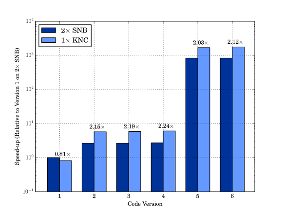
Figure 1: Performance improvement of Modal2D from optimisation and modernisation. The numbers above each of the bars are the performance difference between a coprocessor and two processors for that version.

Table 2: Execution times of Modal2D at various stages of code optimisation.

Version	2$\times\mbox{ }$SNB (s)	1$\times\mbox{ }$KNC (s)	Comment
1	$182005.17$	$225028.22$	Original code.
2	$68748.59$	$31906.09$	Unroll and vectorize loop.
3	$68628.19$	$31304.09$	Memory alignment.
4	$67303.79$	$30100.08$	Remove repeated calculations.
5	$219.0$	$108.0$	New algorithm.
6	$219.0$	$103.33$	Reduce number of threads per core to 2 on KNC.

The graph in Figure 1 shows the speed-up resulting from each of our optimisations and modernisations. For the original code following re-factoring and the introduction of threads (Version 1) we see that KNC is out-performed by two SNB sockets. However, tuning to ensure efficient use of vectors (Versions 2–4) is sufficient to invert this relationship, and highlights the importance of achieving high SIMD efficiency on KNC. The most significant speed-ups arise from algorithmic change (Version 5) on both processor and coprocessor. On KNC we also show that using less threads per core can give a boost in performance for this case (Version 6). (See Table 2.)

3.2 Modal3D

In the original Modal3D code we perform a brute force computation of Equation 2.1, which we repeat here for clarity

$$\Gamma^{\prime}_{nn^{\prime}}=\left\langle Q_{n}\widetilde{Q}_{n^{\prime}}\right\rangle =\sum_{\ell_{1}=2}^{\ell_{max}}\sum_{\ell_{2}=2}^{\ell_{max}}\sum_{\ell_{3}=2}^{\ell_{max}}\frac{\theta_{\ell_{1}\ell_{2}\ell_{3}}}{72\pi^{2}}\frac{(2\ell_{1}+1)(2\ell_{2}+1)(2\ell_{3}+1)(L+1/3)}{(L+1)(L_{1}+1/3)(L_{2}+1/3)(L_{3}+1/3)v_{\ell_{1}}v_{\ell_{2}}v_{\ell_{3}}}$$

$$\times\sqrt{\frac{(L_{1}+1/6)(L_{2}+1/6)(L_{3}+1/6)}{(L+1/6)C_{\ell_{1}}C_{\ell_{2}}C_{\ell_{3}}}}\left(q_{i}(\ell_{1})q_{j}(\ell_{2})q_{k}(\ell_{3})+5\,\mbox{perms}\right)$$

$$\times\int r^{2}dr\left(\tilde{q}_{i^{\prime}}(r,\ell_{1})\tilde{q}_{j^{\prime}}(r,\ell_{2})\tilde{q}_{k^{\prime}}(r,\ell_{3})+5\,\mbox{perms}\right)$$ (12)

The majority of the time is spent in the loop structure shown in Listing 2. The outer loop(n) iterates over rows of $\Gamma$ as the computation of the projected primordial modes, $\tilde{Q}$, done by $\ell$-triple by calculate_xint (which includes the $r$ integration) is the most expensive operation. All pre-factors in $\ell_{i}$, $L_{i}$ and $L$ are calculated and stored in z before we compute the inner product with all the late time modes (calculated by plijk) for the $\ell$-triple. The constraints on the allowed $\ell$-triples give rise to the triangular l1,l2,l3 loops (note the parity constraint in the l3 loop which ensures that the sum of the $\ell_{i}$ is even).

Listing 2: Code snippet for the hotspot in Modal3D.

⬇

for(n=0; n<terms; n++) {

for(l1=0; l1<lsize; l1++) {

for(m=0; m<terms; m++) mvec[m] = 0.0;

for(l2=l1; l2<lsize; l2++) {

for(l3=l2+l1%2; l3<min(l1+l2,lmax)+1; l3+=2) {

x = calculate_xint(l1,l2,l3,n,xsize,xvec,yvec,task);

…

z = permsix(l1,l2,l3)*calculate_geometric(l1,l2,l3)/sqrt(s1*s2*s3);

for(m=0;m<terms;m++) {

y = plijk(m,l1,l2,l3);

mvec[m] += x*y*z;

}

}

}

}

// array reduction of mvec into gamma matrix

}

3.2.1 Threading

As with Modal2D, the original code is parallelised with MPI only over the n loop, and introducing threading via OpenMP is a necessary step to improving utilisation of KNC’s many-core architecture. However, in the 3D variant there are multiple candidate loops that could be parallelised with OpenMP. The inner-most m loop best matches the approach taken in the 2D case, but would be an unwise choice here (since the calculation of x and z would not benefit from parallelisation). Threading the $\ell_{1}\ell_{2}\ell_{3}$ loops instead would be a better idea, if not for the fact that the loop space is triangular; threading only one of the loops would lead either to work imbalance or an iteration count too small to fully utilize all of the available cores.

Ideally we would like to flatten the whole $\ell_{1}\ell_{2}\ell_{3}$ space into a single loop, similar to the effect of OpenMP’s collapse(3) construct. Use of this construct is illegal here, since the number of iterations of the inner loops depends on the indices of the inner loops [23]. We experimented with many different approaches of achieving good load balance using standard OpenMP: spawning separate OpenMP tasks for groups of loop iterations; recursively partitioning the iteration space; and using dynamic scheduling with a threaded outer-loop. In all cases we found that the overheads of these methodologies was significant, the load imbalance was not necessarily adequately addressed, and cache behaviour suffered due to the inability to specify thread affinities. The Intel^® Threading Building Blocks [24] (TBB) library provides task-affinity functionality that may have assisted us with this last point, but we have two reasons for not using it: first, to keep Modal as a C (rather than C++) application; and second, to ensure that our threaded version did not depend heavily on non-standard language features and libraries.

Figure 2: Diagram explaining how we collapse the three loops into a single iteration space.

Instead, we carve up the iteration space manually across tasks, and assign contiguous “chunks” of loop iterations to each thread. This scheme (demonstrated in Figure 2) allows us to achieve very good load balancing at the expense of a small one-time setup overhead. Note that this method is scalable beyond threads – we can manually carve up the total $mn\ell_{1}\ell_{2}\ell_{3}$ iteration space across MPI, then across sockets/coprocessors and finally across threads – which allows us to improve the multi-node scalability of the code.

While restructuring the loop for parallelism, we brought the $n$ loop inside of the $\ell_{1}\ell_{2}\ell_{3}$ nest to reduce the amount of redundant work per thread. However, this increases the amount of temporary storage required by each thread to store its own partial result of $\Gamma_{mn}$. The size of this storage increases by the square of the number of terms, and is $\mathcal{O}(10\mbox{~{}MB})$ for a typical problem size. Assuming 4 threads per core, the amount of temporary storage far exceeds the 512 KB capacity of KNC’s L2 cache, and we see performance degradation due to thrashing effects. If all the threads on one core collaborate to read and write to the same array, then the size of this temporary storage is reduced by a factor of 4 – while it still doesn’t fit in the cache, blocking the loop to compute $B$ iterations between accesses can amortize the bandwidth overheads.

Collaboration between threads in this way requires a “nested” parallelism model, with a 2-tier hierarchy of threads (e.g. $C$ groups of 4 threads, where $C$ is the number of cores). A naïve implementation of nested parallelism in OpenMP is not practical here because the cost of creating and destroying new teams of threads for each iteration of the inner loop is prohibitively expensive. Instead, we adopt an approach where the threads in both tiers are spawned together, and work is assigned to threads based on a combination of their team id (i.e tid / 4) and local worker id (i.e. tid % 4) – all threads execute the same set of $\ell_{1}\ell_{2}\ell_{3}$ loop iterations as the other threads in their group, but execute for different eigenmodes inside the angular momentum loop.

Listing 3: Example implementation of a fast, on-core, barrier.

⬇

typedef __declspec(align(64)) struct corebarrier_t

{

volatile int barrier[2];

int padding[14];

} corebarrier_t;

typedef __declspec(align(64)) struct barrier_t

{

int barrier_id; // which barrier to use this time (0 or 1)

int core_tid; // local thread id on the core (tid % 4)

int flag[2]; // value to write this time (0 or 1)

int waitval; // value to wait on if threads are writing 1s

corebarrier_t* me; // corebarrier_t shared by all threads on the core

} barrier_t;

void cpu_pause()

{

// pause, sleep, or delay this thread

}

void corebarrier(barrier_t *bar)

{

// determine which barrier and values to use

int barrier_id = bar->barrier_id;

int core_tid = bar->core_tid;

int flag = bar->flag[barrier_id];

int waitval = (flag) ? bar->waitval : 0;

// loop until all threads have written to this barrier

corebarrier_t *me = bar->me;

((char *)&me->barrier[barrier_id])[core_tid] = flag;

while (me->barrier[barrier_id] != waitval)

cpu_pause();

// toggle the barrier/flag for next time

bar->flag[barrier_id] = 1 - flag;

bar->barrier_id = 1 - barrier_id;

}

Although this manual nesting approach gives us a great deal of flexibility, it depends on a custom on-core barrier (such as the one shown in Listing 3) to synchronize only the threads in a particular group. There are two reasons to use a local barrier instead of the global barrier provided by OpenMP: first, a global barrier scales $O(log_{2}(4C))$, whereas a local barrier has a constant overhead of $O(4)$; and second, a global barrier can easily lead to accidental deadlocks, since all threads in all groups must be present for all barriers.

3.2.2 Algorithmic Change

The bottleneck left in the code after the loop modernisation is the integration routine called by calculate_xint. This is a 1D integral of a function $f(r)$ with respect to the radial direction along the line of sight, $r$ from now back to the time of inflation. These functions are highly peaked at $r\approx 14,000$, around the time the CMB was formed, and are relatively flat everywhere else. To decrease computational cost and memory consumption, these functions are sampled with 3 different resolutions in $r$, with more points around the surface of last recombination, and less points in the flat regions. Integration was performed by first fitting a spline to the data points and then integrating using the spline to interpolate points which are missing from the sample. In the original code this procedure is performed by the routine gsl_spline_eval_integ from the GSL, but was replaced with a faster equivalent from the Intel^® MKL. We find that although the method from MKL has better vectorisation than the method from GSL, they both suffer from the same problems – they are too memory intensive (storing a cubic spline in addition to the data) and computationally expensive (solving a set of linear equations).

We find that replacing this procedure with a simpler numerical integration routine can drastically speed-up the application even if it requires a greater number of sample points to achieve the same accuracy. We tried two integration methods for this - a simple application of the Trapezium rule and a method that uses Hermite Cubic spline interpolation. These two methods can compute the integral using local points only, unlike the GSL Spline which needs all points to compute the integral. Local methods are much more amenable to vectorisation and also requires $\mathcal{O}(1)$ temporary storage. The Hermite spline integrator is based on the interpolation of $r$ between points $r_{k}$ and $r_{k+1}$ using a Hermite cubic function:

$$p(r_{k})=(2t^{3}-3t^{2}+1)y_{k}+(t^{3}-2t^{2}+t)(r_{k+1}-{r_{k}})p^{\prime}(r_{k})+(-2t^{3}+3t^{2})y_{k+1}+(t^{3}-t^{2})p^{\prime}(r_{k+1})$$ (13)

Where $t=(r-r_{k})/(r_{k+1}-r_{k})$. The exact derivatives of $y(r)$ are not available so we must approximate. Here we use a simple approximation of $p^{\prime}(r_{k})=(y_{k+1}-y_{k})/(x_{k+1}-x_{k})$. Integrating Equation 13 with respect to $r$ and using this derivative yields the integrator:

$$\int dr\;y(r)\approx\frac{1}{2}\sum_{k}\Delta r_{k}\left(y_{k}+y_{k+1}+\frac{1}{6}\Delta r_{k}\left(\frac{\Delta y_{k}}{\Delta r_{k}}-\frac{\Delta y_{k+1}}{\Delta r_{k+1}}\right)\right)$$ (14)

For the results reported here, we use a simple application of the Trapezium rule, combined with 216 sampling points. This scheme has sufficient numerical accuracy for us to obtain a physically meaningful answer, within a few percent of the answer calculated by GSL. Other numerical integration routines (e.g. Gaussian quadrature) may be required for other corner cases, and we leave this investigation to future work.

This leaves two bottlenecks in the code – the partial reduction stage in calculate_gamma_3d, and the calculate_xint routine. The reduction step is actually just a matrix multiply $\Gamma_{mn}=P_{lm}X_{ln}$, and thus it can be replaced with a call to the BLAS-3 DGEMM routine from Intel^® MKL, which is cache-blocked and vectorized efficiently out-of-the-box. We call MKL from only a single thread in each of our nested thread groups, and empirically derive the best blocking factor $B$ to be 64.

3.2.3 Results

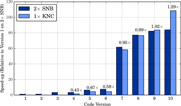
Figure 3: Performance improvement of Modal3D from optimisation and modernisation. The numbers above each of the bars are the performance difference between a coprocessor and two processors for that version.

Table 3: Execution times of Modal3D at various stages of code optimisation.

Version	2$\times\mbox{ }$SNB (s)	1$\times\mbox{ }$KNC (s)	Comment
1	2887.0	-	Original Code.
2	2610.0	-	Loop simplification.
3	882.0	-	MKL Integration. Remove getter methods.
4	865.9	1991.6	Flattened loops + threads.
5	450.6	667.9	Loop reorder, manual nested threading.
6	385.6	655.0	Blocked version of loop.
7	46.9	49.5	Trapezium Integration.
8	37.4	37.7	Reduction with DGEMM.
9	35.1	34.5	Alignment+Padding of Arrays.
10	34.3	26.6	Software Prefetching.

The graph in Figure 3 shows the speed-up resulting from each of our optimisations and modernisations. For the original code following re-factoring and the introduction of threads (Version 1-3) we already see significant gains on the host (3.27$\times\mbox{ }$). Note that we do not provide KNC results until the introduction of OpenMP (Version 4) since we are using the offload model, and offloading work to a single KNC thread does not make sense. Tuning the threading behaviour (Versions 5 and 6) continues to improve performance on both platforms but, as in the case of Modal2D, more significant speed-ups are only possible with algorithmic change – in this case, a change in integration method (Version 7). Further tuning of vectorisation behaviour (Versions 8 and 9) provide a small boost in performance, and tuning the prefetch distance (Version 10) finally pushes the performance of KNC ahead of SNB. (See Table 3.)

Since the same code can be recompiled and ran on both processor and coprocessor, very little effort was required to make the code heterogeneous. We use the asynchronous offload features of Intel^® Language Extensions for Offload (LEO) to offload a fraction (empirically derived to be 71%) of the total problem to KNC, and process the remainder on SNB. On a single node of Cosmic, using KNC in addition to SNB gives a 3.5$\times\mbox{ }$speed-up over using SNB only.

4 Performance Study

The new implementations of the 2D and 3D variants of Modal are optimised but they are not optimal. In this section, we analyze and discuss the remaining bottlenecks to performance at both single- and multi-node scale.

4.1 Integrator Performance: Accuracy vs. Execution Time

In Modal3D, swapping out the spline-based integrator for a simpler one significantly accelerates the code on modern architectures, but at the price of reduce accuracy. We show that this accuracy can be both recovered and increased when using the simpler integrators by increasing the number of sampling points. Moreover, even with a larger sampling size the performance is still likely to be far better than the spline based approach using less points.

Figure 4(a) shows the percentage root mean squared error (RMSE) of the unit normalised $\Gamma$ produced by Modal3D, for different integration methods and different numbers of sample points. We take the result of Modal3D with using the GSL Spline with 1768 sampling points to be the “gold standard” to compare all the others to. All three methods converge towards the gold standard with increasing sample points. The Hermite integrator has nearly identical error to the GSL spline and achieves an error of $<1\times 10^{-5}\%$ of the gold standard with the maximum number of points. The Trapezium integrator is the least accurate of the three, but still gets an error of $<1\times 10^{-4}\%$ of the gold standard. If we consider the accuracies in light of the times to solution shown in Figure 4(b), a clear picture emerges – even after increasing the accuracy of the Hermite and Trapezium integrators, they remain much faster than the GSL spline with a small number of points. The Trapezium integrator is the fastest of the three, but is only $\sim 1.25\times$ faster than the Hermite.

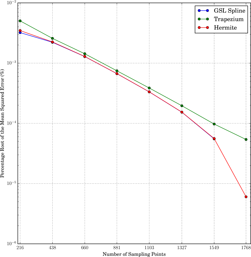
(a) Percentage RMSE of $\Gamma$ using different integrators and numbers of sampling points compared to the GSL Spline method with 1768 sampling points.

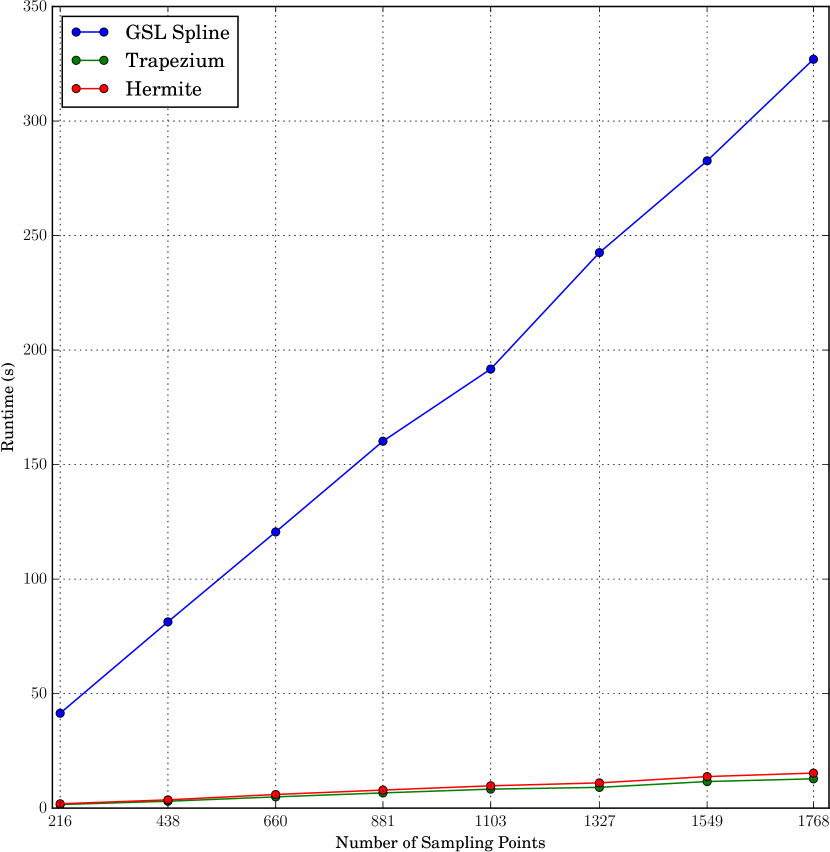
(b) Runtimes of entire Modal3D calculation using different integrators and varying the numbers of sampling points.

Figure 4: Comparison of the accuracy and performance of the different integration methods used in Modal3D.

4.2 Scaling with Cores

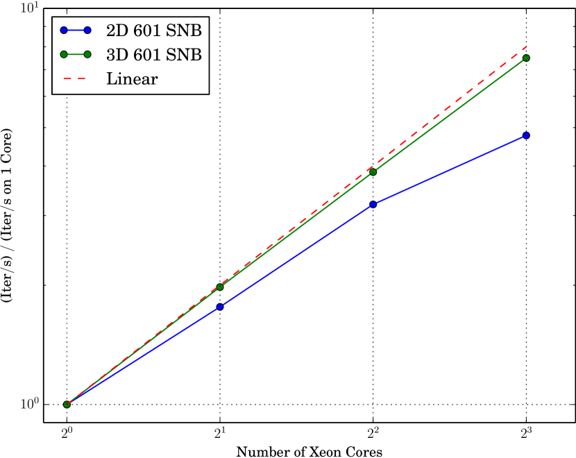
(a) Modal2D

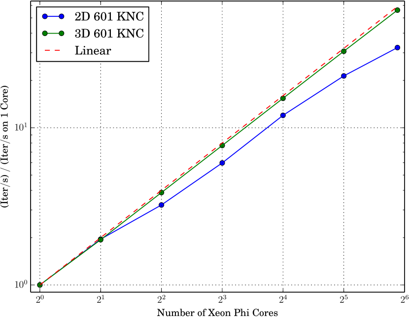
(b) Modal3D

Figure 5: Strong-scaling within a single node, for 601 modes.

Figures 5(a) and 5(b) show how performance of Modal2D and Modal3D scale with the number of cores on SNB and KNC, respectively. The number of threads per core on KNC is fixed at the number that gives the highest performance in each case – 2 and 4 threads per core for Modal2D and Modal3D, respectively.

For Modal2D, we see that scaling tapers off with increasing core-count, reaching a maximum speed-up of 32.4$\times\mbox{ }$. This is not for want of parallel work, nor high synchronisation costs, but rather because the cores are competing for limited memory bandwidth. Running with all 59 cores on KNC, the bandwidth from GDDR to L2 was measured (by Intel VTune Amplifier XE ) to be 147.5 GB/s on average – very close to its peak STREAM [22] bandwidth of 165 GB/s (see Table 1). The fact that we are hitting close to peak shows that there is little room left to further tune the computation performed by Modal2D; any additional work on the 2D variant will need to focus on improving cache locality or algorithmic complexity, not vectorisation.

For Modal3D, we see much better scaling with increasing core-count (close to linear). This is to be expected, since the code is very compute intensive. Furthermore the groups of threads, once spawned, require no communication with each other until the reduction stage at the very end of the calculation. The scaling behaviour suggests that, unlike the 2D variant, Modal3D is not bound by memory bandwidth. However, we are not yet instruction bound, either – running with all 59 cores on KNC, the number of vector instructions issued per cycle was measured by Speedometer [25] to be 39.8% of peak. The performance of Modal3D is in fact limited by transfers between L2 and L1 cache; although there is a large amount of data re-use within a core, the number of streams per thread is too high for the prefetchers to effectively hide the latency of L2 accesses.

4.3 Scaling with Nodes

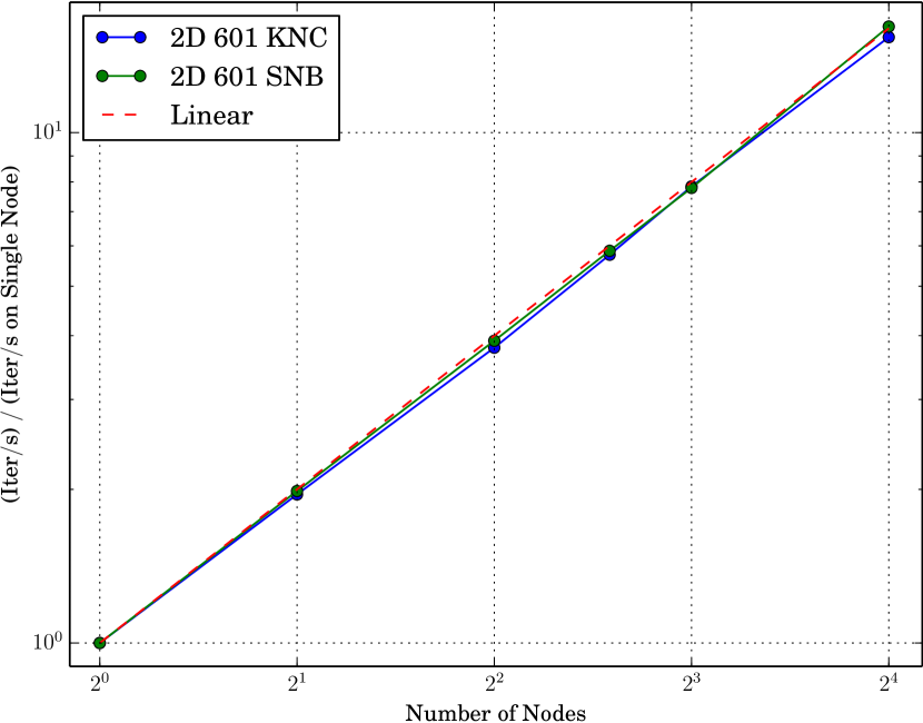
(a) Modal2D

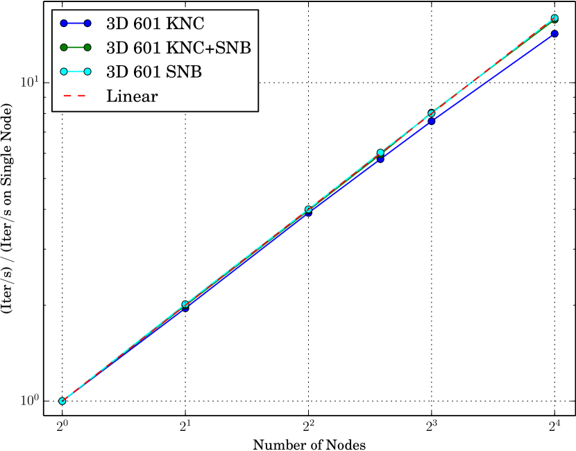
(b) Modal3D

Figure 6: Strong-scaling on multiple nodes, for 601 modes.

Figures 6(a) and 6(b) show how performance scales with the number of Cosmic nodes for Modal2D and Modal3D, respectively. For Modal2D we show results for SNB and KNC alone, while for Modal3D we also show results for a “hybrid” model running 30% of the work on SNB and 70% of the work on KNC. In all cases, we place a single MPI rank per node. The reader is reminded that a single Cosmic node contains only a single SNB socket, and a single KNC coprocessor (see Table 1).

For both the 2D and 3D variants, we see scaling that is fairly close to linear. There are two reasons for this: first, the only communication required between tasks occurs right at the start of a run (to agree on task decomposition) and right at the end (to reduce the final gamma matrix); second, there is a significant amount of work (601 iterations in the 2D case, and $2\times 10^{9}$ iterations in the 3D case) to be split between MPI ranks, so we do not reach a scale where communication costs begin to dominate execution time. Note that although the single-node scaling of Modal2D is inhibited by hardware limitations, this is not the case here – when scaling to multiple nodes, the total available memory bandwidth also scales accordingly.

4.4 Scaling with Problem Size

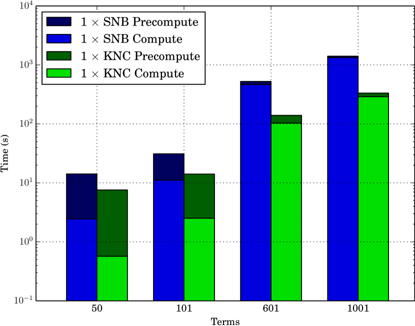
(a) Modal2D

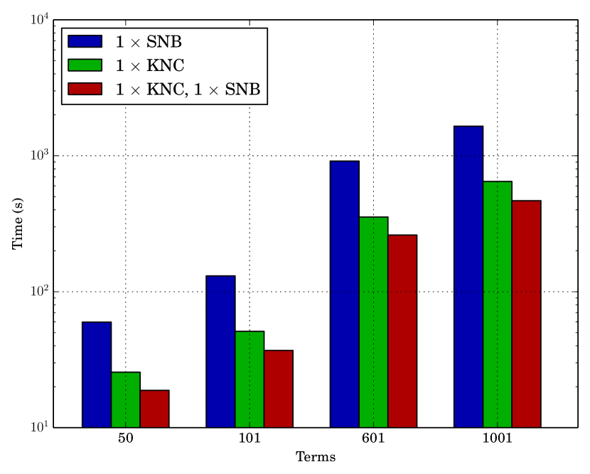
(b) Modal3D

Figure 7: Performance as a function of problem size. In (a) precompute times are stacked on top of the compute times.

Figures 7(a) and 7(b) show how performance scales with problem size for Modal2D and Modal3D, respectively. As in the previous section, we again report performance for three different configurations: SNB alone; KNC alone; and hybrid execution across both processor and coprocessor. Across all variants and problem sizes, KNC beats SNB. Focusing on the 2D variant, the gap between KNC and SNB is largest for large problems. For the two small problems with 50 and 101 terms, the execution time is dominated by the precompute stage of calculation which does not scale well with increasing numbers of threads, and which is thus relatively expensive on KNC. For the larger problems like the 601 and 1001, the execution time is dominated by the real computation of $\Gamma_{mn}$, which is highly scalable on KNC and thus KNC gains and even larger speed-up of 4.1$\times\mbox{ }$over the SNB for the 1001 case.

For the 3D variant, the gap in execution times between SNB and KNC is more consistent, owing to the large amount of parallelism present even in small problems as a result of our fine-grained decomposition of the loops. All the times in 7(b) are for the same $\ell_{1}\ell_{2}\ell_{3}$ space of 18712695 iterations, but for a different number of terms. The amount of computation required in each of Modal3D’s functions scales at different rates with respect to the problem size, and this is reflected in the execution times. The number of eigenmodes that must be integrated scales linearly, but the size of the $Gamma$ matrix and thus the overhead of reducing it scales quadratically. For all the problem sizes we have tested, integration remains the top hotspot, which is why the scaling is close to what one would expect, but the increasing cost of other functions is noticeable.

5 Conclusions

We have presented an optimisation study for the 2D and 3D variants of “Modal”, an early universe simulation and analysis code. It is representative of two common computational challenges: evaluation of a multi-dimensional integral/sum both on a rectangular dense domain, and on a domain which is neither. The optimisation steps detailed here would be applicable to any similar code.

Through a combination of algorithmic improvements, the introduction of thread-level parallelism, and exposing opportunities for hardware vectorisation, we have achieved significant whole application speed-ups: 1765$\times\mbox{ }$on KNC and 833$\times\mbox{ }$on 2$\times\mbox{ }$SNB in the 2D case; and 108$\times\mbox{ }$on KNC and 83.9$\times\mbox{ }$on 2$\times\mbox{ }$SNB in the 3D case. In both cases, the greatest source of speed-up is algorithmic change, and the increased amount of exploitable parallelism it brings. Although still significant, hardware-specific tuning of the new algorithms yields less than 10$\times\mbox{ }$improvement in performance.

Our use of standard programming languages ensures that code changes benefit not only the new Intel Xeon Phi coprocessors, but also Intel Xeon processors – and performance improvements are expected to persist on the next generation of processors and coprocessors (codenamed “Knights Landing”). Investing in code optimisation and modernisation today can deliver significantly greater gains than waiting for future advances in processor technology and will ensure that we maximise the science done on any given architecture.

Appendix A Physics of the Modal code

A.1 Theory

We observe the temperature $T$ of the cosmic microwave background (CMB) on a distant sphere and we can represent anisotropies in this temperature $\Delta T/T$ as

$$\frac{\Delta T}{T}({\bf\hat{n}})=\sum_{lm}a_{lm}Y_{lm}({\bf\hat{n}}).$$ (15)

where $Y_{lm}({\bf\hat{n}})$ are the usual spherical harmonics with multipoles $\ell,m$ with $-\ell\leq m\leq\ell$. Most quantitative cosmology has developed using the two-point correlation or power spectrum $\langle a_{\ell m}a^{*}_{\ell m}\rangle$ defined from a average over the azimuthal multipole $m$

$$C_{\ell}=\frac{1}{2\ell+1}\sum_{m}|a_{\ell m}|^{2}$$ (16)

However, we are interested in new information from the three-point correlator or bispectrum, averaged over orientations as the CMB is assumed isotropic,

$$B_{\ell_{1}\ell_{2}\ell_{3}}=\sum_{m_{i}}\left(\begin{array}[]{ccc}\ell_{1}&\ell_{2}&\ell_{3}\\ m_{1}&m_{2}&m_{3}\end{array}\right)\langle a_{\ell_{1}m_{1}}a_{\ell_{2}m_{2}}a_{\ell_{3}m_{3}}\rangle\,.$$ (19)

This is the spherical respresentation of the 2D CMB bispectrum of triangles on the sky. One of our key goals is to connect this to the 3D primordial bispectrum $\bar{B}(k_{1},k_{2},k_{3})$ generated in the early universe; here, $\bar{B}(k_{1},k_{2},k_{3})$ is defined in terms of wavenumbers $k_{i}$ and must be projected forward using transfer functions describing the evolution of the Universe to predict the late-time $B_{\ell_{1}\ell_{2}\ell_{3}}$.

The modal method is designed to constrain the bispectrum. If you integrate the bispectrum you get the skewness (i.e. how much the distribution leans to one side) of a distribution and, since the bispectrum is zero for a Gaussian distribution, this an effective test of non-Gaussianity. The issue is that the bispectrum is a full three dimensional quantity and so calculating and measuring it is nontrivial. If we wish to constrain a theory which predicts a bispectrum $\bar{B}(k_{1},k_{2},k_{3})$ at the end of inflation, we first need to evolve it forward to today via convolution with transfer functions $\Delta$:

$$B_{\ell_{1}\ell_{2}\ell_{3}}=h_{\ell_{1}\ell_{2}\ell_{3}}\int\bar{B}(k_{1},k_{2},k_{3})\int r^{2}\left(\Pi_{i=1}^{3}\,\Delta_{\ell_{i}}(k_{i})j_{\ell_{i}}(rk_{i})\right)drdk_{1}dk_{2}dk_{3}\,.$$ (20)

where $h$ is a geometric factor related to the projection onto a 2-sphere which will be defined below. This is a 7-dimensional calculation and is impossible in practice. The modal method simplifies this by decomposing the inflationary bispectrum into a set of specially chosen basis functions $\bar{Q}_{n}$ for which this calculation can be dramatically simplified. These $\bar{Q}_{n}$ are defined as:

$$\bar{Q}_{n}(k_{1},k_{2},k_{3}) =\frac{1}{6}\left(\bar{q}_{i}(k_{1})\bar{q}_{j}(k_{2})\bar{q}_{k}(k_{3})+\bar{q}_{j}(k_{1})\bar{q}_{k}(k_{2})\bar{q}_{i}(k_{3})+\bar{q}_{k}(k_{1})\bar{q}_{i}(k_{2})\bar{q}_{j}(k_{3})\right.$$

$$+\left.\bar{q}_{k}(k_{1})\bar{q}_{j}(k_{2})\bar{q}_{i}(k_{3})+\bar{q}_{j}(k_{1})\bar{q}_{i}(k_{2})\bar{q}_{k}(k_{3})+\bar{q}_{i}(k_{1})\bar{q}_{k}(k_{2})\bar{q}_{j}(k_{3})\right)$$ (21)

where the relation between $n$ to $ijk$ is defined via a pre-determined one-to-one mapping which is optimised for convergence. The mapping both is non-analytic and sparse (so not all, or even most, $ijk$ triples correspond to a n) and is read in from a pre-calculated list. An example mapping would look like:

$$\begin{array}[]{lclll}n&\rightarrow&i&j&k\\ \hline\cr 0&\rightarrow&0&0&0\\ 1&\rightarrow&0&0&1\\ 2&\rightarrow&0&1&1\\ 3&\rightarrow&1&1&1\\ 4&\rightarrow&0&0&2\\ 5&\rightarrow&0&1&2\\ \cdots\end{array}$$ (30)

With this basis we then have $\bar{B}^{\prime}=(k_{1}k_{2}k_{3})^{2}\bar{B}=\sum_{n}\bar{\alpha}_{n}\bar{Q}_{n}$ where the $\bar{B}^{\prime}$ is the signal to noise weighted version of $\bar{B}$. The particular form of the basis function allows the projection to be calculated simply and we have:

$$\widetilde{Q}_{n\,\ell_{1}\ell_{2}\ell_{3}} \equiv\frac{1}{6}\int r^{2}dr\left(\tilde{q}_{i}(r,\ell_{1})\tilde{q}_{j}(r,\ell_{2})\tilde{q}_{k}(r,\ell_{3})+5\,\mbox{permutations}\right)$$ (31)

$$\tilde{q}_{i}(x,\ell) \equiv\int dkk^{2}\bar{q}_{i}(k)\Delta_{\ell}(k)\,j_{\ell}(kr)$$ (32)

and now $B_{\ell_{1}\ell_{2}\ell_{3}}=\sum_{n}\bar{\alpha}_{n}\widetilde{Q}_{n}$ and the convolution is effectively 2-dimensional. However this form still proves difficult to use for estimation because of the radial integral $r$ (i.e. distance from inflation to now, along a line of sight). It is more efficient to use a second basis at the time of observation:

$$Q_{n\,\ell_{1}\ell_{2}\ell_{3}} =\frac{1}{6}\left(q_{i}(\ell_{1})q_{j}(\ell_{2})q_{k}(\ell_{3})+q_{j}(\ell_{1})q_{k}(\ell_{2})q_{i}(\ell_{3})+q_{k}(\ell_{1})q_{i}(\ell_{2})q_{j}(\ell_{3})\right.$$

$$+\left.q_{k}(\ell_{1})q_{j}(\ell_{2})q_{i}(\ell_{3})+q_{j}(\ell_{1})q_{i}(\ell_{2})q_{k}(\ell_{3})+q_{i}(\ell_{1})q_{k}(\ell_{2})q_{j}(\ell_{3})\right)\,,$$ (33)

and to project a signal to noise weighted version of the $\widetilde{Q}$ into this new basis, so that we have

$$Q_{n}=\sum_{m}\Gamma_{nm}\widetilde{Q}^{\prime}_{m}=\sum_{m}\Gamma_{nm}\frac{v_{1}v_{2}v_{3}}{\sqrt{C_{\ell_{1}}C_{\ell_{2}}C_{\ell_{3}}}}\widetilde{Q}_{m}$$ (34)

where the $v_{i}=(2\ell+1)^{1/6}$. If we define the inner product (which is designed to mimic the signal to noise structure of the estimator) as:

$$\left\langle A,\,B\right\rangle_{l} \equiv\sum_{\ell_{i}}\ \left(\frac{h_{\ell_{1}\ell_{2}\ell_{3}}}{v_{\ell_{1}}v_{\ell_{2}}v_{\ell_{3}}}\right)^{2}\,A_{\ell_{1}\ell_{2}\ell_{3}}\,B_{\ell_{1}\ell_{2}\ell_{3}}\,,$$ (35)

where $h$ the previously mentioned geometric factor defined by

$$h^{2}_{\ell_{1}\ell_{2}\ell_{3}}=\frac{(2\ell_{1}+1)(2\ell_{2}+1)(2\ell_{3}+1)}{4\pi}\left(\begin{array}[]{ccc}\ell_{1}&\ell_{2}&\ell_{3}\\ 0&0&0\end{array}\right)^{2}\,.$$ (38)

Using this we can then define $\Gamma$ in terms of the inner product as:

$$\Gamma_{nm}=\sum_{r}\left\langle Q_{n},Q_{r}\right\rangle^{-1}\left\langle Q_{r},\widetilde{Q}_{m}\right\rangle$$ (39)

Thus for optimising the calculation of $\Gamma$ we only need to focus on optimising the evaluation of the inner product. The majority of the calculation time is in evaluation the second inner product due to the radial integral inherent in $\widetilde{Q}$, so we will restrict our attention to that part alone defining

$$\Gamma^{\prime}_{nm}=\left\langle Q_{r},\widetilde{Q}_{m}\right\rangle$$ (40)

which is Equation 2.1. The reader is referred to [11] and [12] for a full explanation of the physics.

References

- [1] E. Martinez-Gonzalez, Julio E. Gallegos, F. Argueso, L. Cayon, and J.L. Sanz. The Performance of spherical wavelets to detect non-Gaussianity in the CMB sky. Mon.Not.Roy.Astron.Soc., 336:22, 2002.
- [2] J.-P. Antoine and P. Vandergheynst. Wavelets on the n-sphere and related manifolds. Journal of Mathematical Physics, 39:3987–4008, August 1998.
- [3] L. Cayon, E. Martinez-Gonzalez, F. Argueso, A.J. Banday, and K.M. Gorski. COBE-DMR constraints on the nonlinear coupling parameter: A Wavelet based method. Mon.Not.Roy.Astron.Soc., 339:1189, 2003.
- [4] X. Lan and D. Marinucci. The needlets bispectrum. Electronic Journal of Statistics, 2:332–367, 2008.
- [5] Ø. Rudjord, F. K. Hansen, X. Lan, M. Liguori, D. Marinucci, and S. Matarrese. Directional Variations of the Non-Gaussianity Parameter f NL. Astrophys.J., 708:1321–1325, January 2010.
- [6] S. Donzelli, F. K. Hansen, M. Liguori, D. Marinucci, and S. Matarrese. On the Linear Term Correction for Needlet/Wavelet Non-Gaussianity Estimators. Astrophys.J., 755:19, August 2012.
- [7] Eiichiro Komatsu, David N. Spergel, and Benjamin D. Wandelt. Measuring primordial non-Gaussianity in the cosmic microwave background. Astrophys.J., 634:14–19, 2005.
- [8] E. Komatsu et al. First year Wilkinson Microwave Anisotropy Probe (WMAP) observations: tests of gaussianity. Astrophys.J.Suppl., 148:119–134, 2003.
- [9] Martin Bucher, Bartjan Van Tent, and Carla Sofia Carvalho. Detecting Bispectral Acoustic Oscillations from Inflation Using a New Flexible Estimator. 2009.
- [10] M. Münchmeyer, F. Bouchet, M. G. Jackson, and B. Wandelt. The Komatsu Spergel Wandelt estimator for oscillations in the cosmic microwave background bispectrum. A&A, 570:A94, October 2014.
- [11] JR Fergusson and Edward PS Shellard. Primordial non-gaussianity and the cmb bispectrum. Physical Review D, 76(8):083523, 2007.
- [12] JR Fergusson, M Liguori, and EPS Shellard. General cmb and primordial bispectrum estimation: Mode expansion, map making, and measures of f nl. Physical Review D, 82(2):023502, 2010.
- [13] P.A.R. Ade et al. Planck 2013 Results. XXIV. Constraints on primordial non-Gaussianity. Astron.Astrophys., 571:A24, 2014.
- [14] P.A.R. Ade et al. Planck 2015 results. XVII. Constraints on primordial non-Gaussianity. 2015.
- [15] S. J. Pennycook, Christopher J. Hughes, Mikhail Smelyanskiy, and S. A. Jarvis. Exploring SIMD for Molecular Dynamics, Using Intel Xeon Processors and Intel Xeon Phi Coprocessors. In Proceedings of the IEEE International Parallel and Distributed Processing Symposium, IPDPS ’13, Boston, MA, May 2013.
- [16] Md. Mostafa Ali Patwaray, Nadathur Satish, Narayanan Sundaram, Fredrik Manne, Salman Habib, and Pradeep Dubey. PARDICLE: Parallel Aproximate Density-based Clustering. In Proceedings of the International Conference for High Performance Computing, Networking, Storage and Analysis (SC), SC ’14, New Orleans, LA, November 2014.
- [17] Sanchit Misra, Kiran Pamnany, and Srinivas Aluru. Parallel Mutual Information Based Construction of Whole-Genome Networks on the Intel Xeon Phi Coprocessor. In Proceedings of the IEEE International Parallel and Distributing Processing Symposium, IPDPS ’14, Phoenix, AZ, May 2014.
- [18] Balint Joo, Dhiraj D. Kalamkar, Karthikeyan Vaidyanathan, Mikhail Smelyanskiy, Kiran Pamnany, Victor W. Lee, Pradeep Dubey, and William Watson. Lattice QCD on Intel Xeon Phi Coprocessors. In Proceedings of the IEEE International Supercomputing Conference, ISC ’13, Leipzig, Germany, June 2013.
- [19] Edoardo Apra, Michael Klemm, and Karol Kowalski. Efficient implementation of many-body quantum chemical methods on the intel® xeon phi™ coprocessor. In Proceedings of the International Conference for High Performance Computing, Networking, Storage and Analysis, pages 674–684. IEEE Press, 2014.
- [20] Nicholas Hale and Alex Townsend. Fast and accurate computation of gauss–legendre and gauss–jacobi quadrature nodes and weights. SIAM Journal on Scientific Computing, 35(2):A652–A674, 2013.
- [21] James Jeffers and James Reinders. Intel Xeon Phi coprocessor high-performance programming. Newnes, 2013.
- [22] John D. McCalpin. Memory Bandwidth and Machine Balance in Current High Performance Computers. IEEE Computer Society Technical Committee on Computer Architecture (TCCA) Newsletter, pages 19–25, December 1995.
- [23] OpenMP Architecture Review Board. OpenMP application program interface version 4.0, 2013.
- [24] James Reinders. Intel threading building blocks: outfitting C++ for multi-core processor parallelism. ” O’Reilly Media, Inc.”, 2007.
- [25] Larry Meadows. Speedometer: How fast is your code? https://01.org/simple-performance-tools/documentation/speedometer. Accessed: March 2015.