1 Introduction
The nonlinear wave equation
u t t − c ( u ) ( c ( u ) u x ) x = 0 , subscript 𝑢 𝑡 𝑡 𝑐 𝑢 subscript 𝑐 𝑢 subscript 𝑢 𝑥 𝑥 0 u_{tt}-c(u)\big{(}c(u)u_{x}\big{)}_{x}~{}=~{}0\,, (1.1)
provides a mathematical model for the behavior of
nematic liquid crystals.
Solutions have been studied
by several authors [1 , 2 , 3 , 4 , 7 , 10 , 12 , 13 ] . We recall that, even for smooth initial data
u ( x , 0 ) = u 0 ( x ) , u t ( x , 0 ) = u 1 ( x ) , formulae-sequence 𝑢 𝑥 0 subscript 𝑢 0 𝑥 subscript 𝑢 𝑡 𝑥 0 subscript 𝑢 1 𝑥 u(x,0)~{}=~{}u_{0}(x)\,,\qquad\qquad u_{t}(x,0)~{}=~{}u_{1}(x)\,, (1.2)
regularity can be lost in finite time.
More precisely, the H 1 superscript 𝐻 1 H^{1} u ( ⋅ , t ) 𝑢 ⋅ 𝑡 u(\cdot,t) u 𝑢 u ‖ u x ( ⋅ , t ) ‖ 𝐋 ∞ subscript norm subscript 𝑢 𝑥 ⋅ 𝑡 superscript 𝐋 \|u_{x}(\cdot,t)\|_{{\bf L}^{\infty}}
The paper [4 ] introduced a nonlinear
transformation
of variables that reduces (1.1
w ≐ 2 arctan ( u t + c ( u ) u x ) , z ≐ 2 arctan ( u t − c ( u ) u x ) , formulae-sequence approaches-limit 𝑤 2 subscript 𝑢 𝑡 𝑐 𝑢 subscript 𝑢 𝑥 approaches-limit 𝑧 2 subscript 𝑢 𝑡 𝑐 𝑢 subscript 𝑢 𝑥 w~{}\doteq~{}2\arctan\bigl{(}u_{t}+c(u)u_{x}\bigr{)},\qquad\qquad z~{}\doteq~{}2\arctan\bigl{(}u_{t}-c(u)u_{x}\bigr{)},
satisfy a first order semilinear system of equations, w.r.t. new
independent variables X 𝑋 X Y 𝑌 Y x , t , u 𝑥 𝑡 𝑢
x,t,u 1.1
Based on this representation and using ideas from
[5 , 6 , 8 , 9 ] , in [1 ] it was recently
proved that,
for generic initial data,
the conservative solution is smooth outside a finite
number of points and curves in the t 𝑡 t x 𝑥 x structural stability of the set of singularities.
Namely, when these generic
conditions hold, the topological structure of the singular set
is not affected by a small 𝒞 3 superscript 𝒞 3 {\mathcal{C}}^{3}
Aim of the present paper is to derive a detailed asymptotic
description of these structurally stable solutions,
in a neighborhood of each singular point.
This is achieved both for conservative and for dissipative solutions
of (1.1
ℰ ( t ) = 1 2 ∫ [ u t 2 + c 2 ( u ) u x 2 ] 𝑑 x ℰ 𝑡 1 2 delimited-[] superscript subscript 𝑢 𝑡 2 superscript 𝑐 2 𝑢 superscript subscript 𝑢 𝑥 2 differential-d 𝑥 {\mathcal{E}}(t)~{}=~{}{1\over 2}\int[u_{t}^{2}+c^{2}(u)u_{x}^{2}]\,dx
coincides with a constant for a.e. time t 𝑡 t [3 ] .
The remainder of this paper is organized as follows. In Section 2
we review the variable transformations introduced in [4 ]
and the conditions for structural stability derived in [1 ] .
Section 3 is concerned with conservative solutions.
In this case, for smooth initial data the map
( X , Y ) ↦ ( x , t , u , w , z ) ( X , Y ) maps-to 𝑋 𝑌 𝑥 𝑡 𝑢 𝑤 𝑧 𝑋 𝑌 (X,Y)~{}\mapsto~{}(x,t,u,w,z)(X,Y) (1.3)
remains globally smooth, on the entire
X 𝑋 X Y 𝑌 Y u ( x , t ) 𝑢 𝑥 𝑡 u(x,t) 1.1 1.3 w = π 𝑤 𝜋 w=\pi z = π 𝑧 𝜋 z=\pi
We remark that, for conservative solutions,
a general uniqueness theorem
has been recently established in [2 ] .
On the other hand, for dissipative solutions no general
result on uniqueness or continuous dependence is yet known.
Whether structurally stable dissipative solutions are generic ,
arising from an open dense set of 𝒞 3 superscript 𝒞 3 {\mathcal{C}}^{3}
2 Review of the equations
Throughout the following, on the wave speed c 𝑐 c
(A)
The map
c : ℝ ↦ ℝ + : 𝑐 maps-to ℝ subscript ℝ c:{\mathbb{R}}\mapsto{\mathbb{R}}_{+} c ′ ( u ) / c ( u ) superscript 𝑐 ′ 𝑢 𝑐 𝑢 c^{\prime}(u)/c(u)
c ′ ( u ) = 0 ⟹ c ′′ ( u ) ≠ 0 . formulae-sequence superscript 𝑐 ′ 𝑢 0
superscript 𝑐 ′′ 𝑢 0 c^{\prime}(u)~{}=~{}0\qquad\implies\qquad c^{\prime\prime}(u)~{}\not=~{}0. (2.1)
Because of (2.1 c ′ ( u ) superscript 𝑐 ′ 𝑢 c^{\prime}(u)
In (1.2 ( u 0 , u 1 ) subscript 𝑢 0 subscript 𝑢 1 (u_{0},u_{1}) H 1 ( ℝ ) × 𝐋 2 ( ℝ ) superscript 𝐻 1 ℝ superscript 𝐋 2 ℝ H^{1}({\mathbb{R}})\times{\bf L}^{2}({\mathbb{R}})
{ R ≐ u t + c ( u ) u x , S ≐ u t − c ( u ) u x , cases 𝑅 approaches-limit subscript 𝑢 𝑡 𝑐 𝑢 subscript 𝑢 𝑥 𝑆 approaches-limit subscript 𝑢 𝑡 𝑐 𝑢 subscript 𝑢 𝑥 \left\{\begin{array}[]{rcl}R&\doteq&u_{t}+c(u)u_{x}\,,\\
S&\doteq&u_{t}-c(u)u_{x}\,,\end{array}\right. (2.2)
In a smooth solution, R 2 superscript 𝑅 2 R^{2} S 2 superscript 𝑆 2 S^{2}
{ ( R 2 ) t − ( c R 2 ) x = c ′ 2 c ( R 2 S − R S 2 ) , ( S 2 ) t + ( c S 2 ) x = c ′ 2 c ( S 2 R − S R 2 ) . cases subscript superscript 𝑅 2 𝑡 subscript 𝑐 superscript 𝑅 2 𝑥 superscript 𝑐 ′ 2 𝑐 superscript 𝑅 2 𝑆 𝑅 superscript 𝑆 2 subscript superscript 𝑆 2 𝑡 subscript 𝑐 superscript 𝑆 2 𝑥 superscript 𝑐 ′ 2 𝑐 superscript 𝑆 2 𝑅 𝑆 superscript 𝑅 2 \left\{\begin{array}[]{rcl}(R^{2})_{t}-(cR^{2})_{x}&=&{c^{\prime}\over 2c}(R^{2}S-RS^{2})\,,\\[8.53581pt]
(S^{2})_{t}+(cS^{2})_{x}&=&{c^{\prime}\over 2c}(S^{2}R-SR^{2})\,.\end{array}\right. (2.3)
As a consequence, the energy is conserved:
E ≐ 1 2 ( u t 2 + c 2 u x 2 ) = R 2 + S 2 4 , approaches-limit 𝐸 1 2 superscript subscript 𝑢 𝑡 2 superscript 𝑐 2 superscript subscript 𝑢 𝑥 2 superscript 𝑅 2 superscript 𝑆 2 4 E~{}\doteq~{}{1\over 2}\big{(}u_{t}^{2}+c^{2}u_{x}^{2}\big{)}~{}=~{}{R^{2}+S^{2}\over 4}\,, (2.4)
One can think of R 2 superscript 𝑅 2 R^{2} S 2 superscript 𝑆 2 S^{2} 2.3
A major difficulty in the analysis of (1.1 u x , u t subscript 𝑢 𝑥 subscript 𝑢 𝑡
u_{x},u_{t} R , S 𝑅 𝑆
R,S [4 ]
we introduce a new set of dependent variables:
w ≐ 2 arctan R , z ≐ 2 arctan S . formulae-sequence approaches-limit 𝑤 2 𝑅 approaches-limit 𝑧 2 𝑆 w~{}\doteq~{}2\arctan R\,,\qquad\qquad z~{}\doteq~{}2\arctan S\,. (2.5)
Figure 1: The backward and forward characteristic
through the point ( x , t ) 𝑥 𝑡 (x,t)
To reduce the equation (1.1 1
x ˙ + = c ( u ) , x ˙ − = − c ( u ) . formulae-sequence superscript ˙ 𝑥 𝑐 𝑢 superscript ˙ 𝑥 𝑐 𝑢 \dot{x}^{+}=c(u)\,,\qquad\qquad\dot{x}^{-}=-c(u)\,. (2.6)
The characteristics passing through the point ( x , t ) 𝑥 𝑡 (x,t)
s ↦ x + ( s , x , t ) , s ↦ x − ( s , x , t ) , formulae-sequence maps-to 𝑠 superscript 𝑥 𝑠 𝑥 𝑡 maps-to 𝑠 superscript 𝑥 𝑠 𝑥 𝑡 s\mapsto x^{+}(s,x,t)\,,\qquad\qquad s\mapsto x^{-}(s,x,t)\,,
respectively.
As coordinates ( X , Y ) 𝑋 𝑌 (X,Y) ( x , t ) 𝑥 𝑡 (x,t)
X ≐ x − ( 0 , x , t ) , Y ≐ − x + ( 0 , x , t ) . formulae-sequence approaches-limit 𝑋 superscript 𝑥 0 𝑥 𝑡 approaches-limit 𝑌 superscript 𝑥 0 𝑥 𝑡 X~{}\doteq~{}x^{-}(0,x,t)\,,\qquad\qquad Y~{}\doteq~{}-x^{+}(0,x,t)\,. (2.7)
For future use, we now introduce the further variables
p ≐ 1 + R 2 X x , q ≐ 1 + S 2 − Y x . formulae-sequence approaches-limit 𝑝 1 superscript 𝑅 2 subscript 𝑋 𝑥 approaches-limit 𝑞 1 superscript 𝑆 2 subscript 𝑌 𝑥 p\doteq{1+R^{2}\over X_{x}}\,,\qquad\qquad q\doteq{1+S^{2}\over-Y_{x}}\,. (2.8)
Starting with the nonlinear equation (1.1 X , Y 𝑋 𝑌
X,Y u , w , z , p , q , x , t 𝑢 𝑤 𝑧 𝑝 𝑞 𝑥 𝑡
u,w,z,p,q,x,t
{ u X = sin w 4 c p , u Y = sin z 4 c q , cases subscript 𝑢 𝑋 𝑤 4 𝑐 𝑝 subscript 𝑢 𝑌 𝑧 4 𝑐 𝑞 \left\{\begin{array}[]{ccc}u_{X}&=&{\sin w\over 4c}\,p\,,\\[11.38109pt]
u_{Y}&=&{\sin z\over 4c}\,q\,,\end{array}\right. (2.9)
{ w Y = c ′ 8 c 2 ( cos z − cos w ) q , z X = c ′ 8 c 2 ( cos w − cos z ) p , cases subscript 𝑤 𝑌 superscript 𝑐 ′ 8 superscript 𝑐 2 𝑧 𝑤 𝑞 subscript 𝑧 𝑋 superscript 𝑐 ′ 8 superscript 𝑐 2 𝑤 𝑧 𝑝 \left\{\begin{array}[]{ccc}w_{Y}&=&{c^{\prime}\over 8c^{2}}\,(\cos z-\cos w)\,q\,,\\[11.38109pt]
z_{X}&=&{c^{\prime}\over 8c^{2}}\,(\cos w-\cos z)\,p\,,\end{array}\right. (2.10)
{ p Y = c ′ 8 c 2 ( sin z − sin w ) p q , q X = c ′ 8 c 2 ( sin w − sin z ) p q , cases subscript 𝑝 𝑌 superscript 𝑐 ′ 8 superscript 𝑐 2 𝑧 𝑤 𝑝 𝑞 subscript 𝑞 𝑋 superscript 𝑐 ′ 8 superscript 𝑐 2 𝑤 𝑧 𝑝 𝑞 \left\{\begin{array}[]{ccc}p_{Y}&=&{c^{\prime}\over 8c^{2}}\,(\sin z-\sin w)\,pq\,,\\[11.38109pt]
q_{X}&=&{c^{\prime}\over 8c^{2}}\,(\sin w-\sin z)\,pq\,,\end{array}\right. (2.11)
{ x X = ( 1 + cos w ) p 4 , x Y = − ( 1 + cos z ) q 4 , cases subscript 𝑥 𝑋 1 𝑤 𝑝 4 subscript 𝑥 𝑌 1 𝑧 𝑞 4 \left\{\begin{array}[]{ccr}x_{X}&=&{(1+\cos w)\,p\over 4}\,,\\[11.38109pt]
x_{Y}&=&-{(1+\cos z)\,q\over 4}\,,\end{array}\right. (2.12)
{ t X = ( 1 + cos w ) p 4 c , t Y = ( 1 + cos z ) q 4 c . cases subscript 𝑡 𝑋 1 𝑤 𝑝 4 𝑐 subscript 𝑡 𝑌 1 𝑧 𝑞 4 𝑐 \left\{\begin{array}[]{ccr}t_{X}&=&{(1+\cos w)\,p\over 4c}\,,\\[11.38109pt]
t_{Y}&=&{(1+\cos z)\,q\over 4c}\,.\end{array}\right. (2.13)
See [4 ] for detailed computations.
Boundary data can be assigned on the line
γ 0 = { ( X , Y ) ; X + Y = 0 } subscript 𝛾 0 𝑋 𝑌 𝑋 𝑌
0 \gamma_{0}=\{(X,Y)\,;~{}X+Y=0\}
{ u ( s , − s ) = u ¯ ( s ) , x ( s , − s ) = x ¯ ( s ) , t ( s , − s ) = t ¯ ( s ) , { w ( s , − s ) = w ¯ ( s ) , z ( s , − s ) = z ¯ ( s ) , { p ( s , − s ) = p ¯ ( s ) , q ( s , − s ) = q ¯ ( s ) , cases 𝑢 𝑠 𝑠 absent ¯ 𝑢 𝑠 𝑥 𝑠 𝑠 absent ¯ 𝑥 𝑠 𝑡 𝑠 𝑠 absent ¯ 𝑡 𝑠 cases 𝑤 𝑠 𝑠 absent ¯ 𝑤 𝑠 𝑧 𝑠 𝑠 absent ¯ 𝑧 𝑠 cases 𝑝 𝑠 𝑠 absent ¯ 𝑝 𝑠 missing-subexpression 𝑞 𝑠 𝑠 absent ¯ 𝑞 𝑠 missing-subexpression
\left\{\begin{array}[]{rl}u(s,\,-s)&=~{}\overline{u}(s)\,,\\
x(s,\,-s)&=~{}\overline{x}(s)\,,\\
t(s,\,-s)&=~{}\overline{t}(s)\,,\end{array}\right.\qquad\qquad\left\{\begin{array}[]{rl}w(s,\,-s)&=~{}\overline{w}(s)\,,\\
z(s,\,-s)&=~{}\overline{z}(s)\,,\end{array}\right.\qquad\qquad\left\{\begin{array}[]{rcl}p(s,\,-s)&=~{}\overline{p}(s)\,,\\
q(s,\,-s)&=~{}\overline{q}(s)\,,\end{array}\right. (2.14)
for suitable smooth functions u ¯ , , x ¯ , t ¯ , w ¯ , z ¯ , p ¯ , q ¯ \overline{u},,\overline{x},\overline{t},\overline{w},\overline{z},\overline{p},\overline{q}
Remark 1. The above system is clearly
invariant w.r.t. the addition
of an integer multiple of 2 π 2 𝜋 2\pi w , z 𝑤 𝑧
w,z w , z 𝑤 𝑧
w,z 𝕋 ≐ ℝ / 2 π ℤ approaches-limit 𝕋 ℝ 2 𝜋 ℤ {\mathbb{T}}\doteq{\mathbb{R}}/2\pi{\mathbb{Z}}
w ≠ π ⟹ cos w > − 1 , z ≠ π ⟹ cos z > − 1 . 𝑤 formulae-sequence absent 𝜋
𝑤 1 𝑧 formulae-sequence absent 𝜋
𝑧 1 \begin{array}[]{rl}w&\not=~{}\pi\qquad\implies\qquad\cos w~{}>~{}-1\,,\\[8.53581pt]
z&\not=~{}\pi\qquad\implies\qquad\cos z~{}>~{}-1\,.\end{array} (2.15)
Remark 2. The system (2.9 2.13 u , x , t 𝑢 𝑥 𝑡
u,x,t 2.9 2.13 2.12 [1 ] , in order that all the above equations be
simultaneously satisfied along the line
γ 0 subscript 𝛾 0 \gamma_{0}
d d s u ¯ ( s ) = sin w ¯ ( s ) 4 c ( u ¯ ( s ) ) p ¯ ( s ) − sin z ¯ ( s ) 4 c ( u ¯ ( s ) ) q ¯ ( s ) , 𝑑 𝑑 𝑠 ¯ 𝑢 𝑠 ¯ 𝑤 𝑠 4 𝑐 ¯ 𝑢 𝑠 ¯ 𝑝 𝑠 ¯ 𝑧 𝑠 4 𝑐 ¯ 𝑢 𝑠 ¯ 𝑞 𝑠 {d\over ds}\overline{u}(s)~{}=~{}{\sin\overline{w}(s)\over 4c(\overline{u}(s))}\,\overline{p}(s)-{\sin\overline{z}(s)\over 4c(\overline{u}(s))}\,\overline{q}(s)\,, (2.16)
d d s x ¯ ( s ) = ( 1 + cos q ¯ ( s ) ) p ¯ ( s ) + ( 1 + cos z ¯ ( s ) ) q ¯ ( s ) 4 , 𝑑 𝑑 𝑠 ¯ 𝑥 𝑠 1 ¯ 𝑞 𝑠 ¯ 𝑝 𝑠 1 ¯ 𝑧 𝑠 ¯ 𝑞 𝑠 4 {d\over ds}\overline{x}(s)~{}=~{}{(1+\cos\overline{q}(s))\overline{p}(s)+(1+\cos\overline{z}(s))\overline{q}(s)\over 4}\,, (2.17)
d d s t ¯ ( s ) = ( 1 + cos w ¯ ( s ) ) p ¯ ( s ) − ( 1 + cos z ¯ ( s ) ) q ¯ ( s ) 4 c ( u ¯ ( s ) ) . 𝑑 𝑑 𝑠 ¯ 𝑡 𝑠 1 ¯ 𝑤 𝑠 ¯ 𝑝 𝑠 1 ¯ 𝑧 𝑠 ¯ 𝑞 𝑠 4 𝑐 ¯ 𝑢 𝑠 {d\over ds}\overline{t}(s)~{}=~{}{(1+\cos\overline{w}(s))\overline{p}(s)-(1+\cos\overline{z}(s))\overline{q}(s)\over 4c(\overline{u}(s))}\,. (2.18)
In turn, if (2.16 2.18 γ 0 subscript 𝛾 0 \gamma_{0} 2.9 2.13 X 𝑋 X Y 𝑌 Y ( u 0 , u 1 ) subscript 𝑢 0 subscript 𝑢 1 (u_{0},u_{1}) 1.2 2.14 γ 0 subscript 𝛾 0 \gamma_{0}
{ u ¯ ( x ) = u 0 ( x ) , t ¯ ( x ) = 0 , x ¯ ( x ) = x , { w ¯ ( x ) = 2 arctan R ( x , 0 ) , z ¯ ( x ) = 2 arctan S ( x , 0 ) , { p ¯ ( x ) ≡ 1 + R 2 ( x , 0 ) , q ¯ ( x ) ≡ 1 + S 2 ( x , 0 ) . cases ¯ 𝑢 𝑥 absent subscript 𝑢 0 𝑥 ¯ 𝑡 𝑥 absent 0 ¯ 𝑥 𝑥 absent 𝑥 cases ¯ 𝑤 𝑥 absent 2 𝑅 𝑥 0 ¯ 𝑧 𝑥 absent 2 𝑆 𝑥 0 cases ¯ 𝑝 𝑥 1 superscript 𝑅 2 𝑥 0 ¯ 𝑞 𝑥 1 superscript 𝑆 2 𝑥 0
\left\{\begin{array}[]{rl}\overline{u}(x)&=~{}u_{0}(x)\,,\\
\overline{t}(x)&=~{}0\,,\\
\overline{x}(x)&=~{}x\,,\end{array}\right.\qquad\quad\left\{\begin{array}[]{rl}\overline{w}(x)&=~{}2\arctan R(x,0)\,,\\
\overline{z}(x)&=~{}2\arctan S(x,0)\,,\end{array}\right.\quad\qquad\left\{\begin{array}[]{rcl}\overline{p}(x)&\equiv&1+R^{2}(x,0)\,,\\
\overline{q}(x)&\equiv&1+S^{2}(x,0)\,.\end{array}\right. (2.19)
We recall that, at time t = 0 𝑡 0 t=0 1.2
R ( x , 0 ) = ( u t + c ( u ) u x ) ( x , 0 ) = u 1 ( x ) + c ( u 0 ( x ) ) u 0 , x ( x ) , S ( x , 0 ) = ( u t − c ( u ) u x ) ( x , 0 ) = u 1 ( x ) − c ( u 0 ( x ) ) u 0 , x ( x ) . 𝑅 𝑥 0 absent subscript 𝑢 𝑡 𝑐 𝑢 subscript 𝑢 𝑥 𝑥 0 subscript 𝑢 1 𝑥 𝑐 subscript 𝑢 0 𝑥 subscript 𝑢 0 𝑥
𝑥 𝑆 𝑥 0 absent subscript 𝑢 𝑡 𝑐 𝑢 subscript 𝑢 𝑥 𝑥 0 subscript 𝑢 1 𝑥 𝑐 subscript 𝑢 0 𝑥 subscript 𝑢 0 𝑥
𝑥 \begin{array}[]{lr}R(x,0)&=~{}(u_{t}+c(u)u_{x})(x,0)~{}=~{}u_{1}(x)+c(u_{0}(x))u_{0,x}(x),\\[11.38109pt]
S(x,0)&=~{}(u_{t}-c(u)u_{x})(x,0)~{}=~{}u_{1}(x)-c(u_{0}(x))u_{0,x}(x).\end{array}
As proved in [1 ] ,
for any choice of u 0 , u 1 subscript 𝑢 0 subscript 𝑢 1
u_{0},u_{1} 2.19 2.16 2.18
The following theorems summarize the main results on
conservative solutions, proved in [4 , 1 , 2 ] .
As before, 𝒰 𝒰 {\mathcal{U}} 2.21 Theorem 1. Let the wave speed c ( ⋅ ) 𝑐 ⋅ c(\cdot) (A) .
Given initial data ( u 0 , u 1 ) ∈ H 1 ( ℝ ) × 𝐋 2 ( ℝ ) subscript 𝑢 0 subscript 𝑢 1 superscript 𝐻 1 ℝ superscript 𝐋 2 ℝ (u_{0},u_{1})\in H^{1}({\mathbb{R}})\times{\bf L}^{2}({\mathbb{R}}) ( X , Y ) ↦ ( u , w , z , p , q , x , t ) ( X , Y ) maps-to 𝑋 𝑌 𝑢 𝑤 𝑧 𝑝 𝑞 𝑥 𝑡 𝑋 𝑌 (X,Y)\mapsto(u,w,z,p,q,x,t)(X,Y) 2.9 2.13 2.14 2.19 γ 0 subscript 𝛾 0 \gamma_{0}
Graph ( u ) ≐ { ( x ( X , Y ) , t ( X , Y ) , u ( X , Y ) ) ; ( X , Y ) ∈ ℝ 2 } approaches-limit Graph 𝑢 𝑥 𝑋 𝑌 𝑡 𝑋 𝑌 𝑢 𝑋 𝑌 𝑋 𝑌
superscript ℝ 2 \hbox{\rm Graph}(u)~{}\doteq~{}\Big{\{}\bigl{(}x(X,Y),~{}t(X,Y),~{}u(X,Y)\bigr{)}\,;~{}~{}(X,Y)\in{\mathbb{R}}^{2}\Big{\}} (2.20)
is the graph of the unique conservative solution u = u ( x , t ) 𝑢 𝑢 𝑥 𝑡 u=u(x,t) 1.1 1.2
Theorem 2. Let the assumptions
(A) be satisfied and let T > 0 𝑇 0 T>0
𝒟 ⊂ 𝒰 ≐ ( 𝒞 3 ( ℝ ) ∩ H 1 ( ℝ ) ) × ( 𝒞 2 ( ℝ ) ∩ 𝐋 2 ( ℝ ) ) 𝒟 𝒰 approaches-limit superscript 𝒞 3 ℝ superscript 𝐻 1 ℝ superscript 𝒞 2 ℝ superscript 𝐋 2 ℝ {\mathcal{D}}~{}\subset~{}{\mathcal{U}}~{}\doteq~{}\Big{(}{\mathcal{C}}^{3}({\mathbb{R}})\cap H^{1}({\mathbb{R}})\Big{)}\times\Big{(}{\mathcal{C}}^{2}({\mathbb{R}})\cap{\bf L}^{2}({\mathbb{R}})\Big{)} (2.21)
such that the following holds.
For every initial data ( u 0 , u 1 ) ∈ 𝒟 subscript 𝑢 0 subscript 𝑢 1 𝒟 (u_{0},u_{1})\in{\mathcal{D}} ( u , w , z , p , q , z , t ) 𝑢 𝑤 𝑧 𝑝 𝑞 𝑧 𝑡 (u,w,z,p,q,z,t) 2.9 2.13 2.14 2.19 { w = π } 𝑤 𝜋 \{w=\pi\} { z = π } 𝑧 𝜋 \{z=\pi\}
{ ( w , w X , w X X ) = ( π , 0 , 0 ) , ( z , z Y , z Y Y ) = ( π , 0 , 0 ) , cases 𝑤 subscript 𝑤 𝑋 subscript 𝑤 𝑋 𝑋 absent 𝜋 0 0 𝑧 subscript 𝑧 𝑌 subscript 𝑧 𝑌 𝑌 absent 𝜋 0 0 \left\{\begin{array}[]{rl}(w,w_{X},w_{XX})&=~{}(\pi,0,0),\\[8.53581pt]
(z,z_{Y},z_{YY})&=~{}(\pi,0,0),\end{array}\right. (2.22)
{ ( w , z , w X ) = ( π , π , 0 ) , ( w , z , z Y ) = ( π , π , 0 ) , cases 𝑤 𝑧 subscript 𝑤 𝑋 absent 𝜋 𝜋 0 𝑤 𝑧 subscript 𝑧 𝑌 absent 𝜋 𝜋 0 \left\{\begin{array}[]{rl}(w,z,w_{X})&=~{}(\pi,\pi,0),\\[8.53581pt]
(w,z,z_{Y})&=~{}(\pi,\pi,0),\end{array}\right. (2.23)
{ ( w , w X , c ′ ( u ) ) = ( π , 0 , 0 ) , ( z , z Y , c ′ ( u ) ) = ( π , 0 , 0 ) . cases 𝑤 subscript 𝑤 𝑋 superscript 𝑐 ′ 𝑢 absent 𝜋 0 0 𝑧 subscript 𝑧 𝑌 superscript 𝑐 ′ 𝑢 absent 𝜋 0 0 \left\{\begin{array}[]{rl}(w,w_{X},c^{\prime}(u))&=~{}(\pi,0,0),\\[8.53581pt]
(z,z_{Y},c^{\prime}(u))&=~{}(\pi,0,0).\end{array}\right. (2.24)
is ever attained, at any point ( X , Y ) 𝑋 𝑌 (X,Y)
( x ( X , Y ) , t ( X , Y ) ) ∈ ℝ × [ 0 , T ] . 𝑥 𝑋 𝑌 𝑡 𝑋 𝑌 ℝ 0 𝑇 \bigl{(}x(X,Y),~{}t(X,Y)\bigr{)}~{}\in~{}{\mathbb{R}}\times[0,T]\,. (2.25)
The singularities of the solution
u 𝑢 u x 𝑥 x t 𝑡 t { w = π } 𝑤 𝜋 \{w=\pi\} { z = π } 𝑧 𝜋 \{z=\pi\}
Λ : ( X , Y ) ↦ ( x ( X , Y ) , t ( X , Y ) ) . : Λ maps-to 𝑋 𝑌 𝑥 𝑋 𝑌 𝑡 𝑋 𝑌 \Lambda:(X,Y)~{}\mapsto~{}\bigl{(}x(X,Y),~{}t(X,Y)\bigr{)}. (2.26)
If none of the values
in (2.22 2.24 𝒞 2 superscript 𝒞 2 {\mathcal{C}}^{2} X 𝑋 X Y 𝑌 Y ℝ × [ 0 , T ] ℝ 0 𝑇 {\mathbb{R}}\times[0,T] u 𝑢 u 𝒞 2 superscript 𝒞 2 {\mathcal{C}}^{2} x 𝑥 x t 𝑡 t
Figure 2: Two level sets { w = π } 𝑤 𝜋 \{w=\pi\} { z = π } 𝑧 𝜋 \{z=\pi\} 2.9 2.11 P 𝑃 P P 1 subscript 𝑃 1 P_{1} P 2 subscript 𝑃 2 P_{2} P 3 subscript 𝑃 3 P_{3} Q 1 subscript 𝑄 1 Q_{1} Q 2 subscript 𝑄 2 Q_{2} P 1 subscript 𝑃 1 P_{1} Y ( X ) 𝑌 𝑋 Y(X) w ( X , Y ( X ) ) = π 𝑤 𝑋 𝑌 𝑋 𝜋 w(X,Y(X))=\pi Q 1 subscript 𝑄 1 Q_{1} Q 2 subscript 𝑄 2 Q_{2} 2.10 w Y = z X = 0 subscript 𝑤 𝑌 subscript 𝑧 𝑋 0 w_{Y}=z_{X}=0 { w = π } 𝑤 𝜋 \{w=\pi\} { z = π } 𝑧 𝜋 \{z=\pi\} Figure 3: The images of the level sets
{ w = π } 𝑤 𝜋 \{w=\pi\} { z = π } 𝑧 𝜋 \{z=\pi\} 2 Λ : ( X , Y ) ↦ ( x ( X , Y ) , t ( X , Y ) ) : Λ maps-to 𝑋 𝑌 𝑥 𝑋 𝑌 𝑡 𝑋 𝑌 \Lambda:(X,Y)\mapsto(x(X,Y),t(X,Y)) x 𝑥 x t 𝑡 t u = u ( x , t ) 𝑢 𝑢 𝑥 𝑡 u=u(x,t) 1.1 u x → ± ∞ → subscript 𝑢 𝑥 plus-or-minus u_{x}\to\pm\infty p 1 , p 2 , p 3 subscript 𝑝 1 subscript 𝑝 2 subscript 𝑝 3
p_{1},p_{2},p_{3} q 1 , q 2 subscript 𝑞 1 subscript 𝑞 2
q_{1},q_{2}
3 Singularities of conservative solutions
For smooth data u 0 , u 1 ∈ 𝒞 ∞ ( ℝ ) subscript 𝑢 0 subscript 𝑢 1
superscript 𝒞 ℝ u_{0},u_{1}\in{\mathcal{C}}^{\infty}({\mathbb{R}}) ( X , Y ) ↦ ( x , t , u , w , z , p , q ) ( X , Y ) maps-to 𝑋 𝑌 𝑥 𝑡 𝑢 𝑤 𝑧 𝑝 𝑞 𝑋 𝑌 (X,Y)\mapsto(x,t,u,w,z,p,q)(X,Y) 2.9 2.13 2.14 2.19 X 𝑋 X Y 𝑌 Y u = u ( x , t ) 𝑢 𝑢 𝑥 𝑡 u=u(x,t) 1.1 Λ : ( X , Y ) ↦ ( x , t ) : Λ maps-to 𝑋 𝑌 𝑥 𝑡 \Lambda:(X,Y)\mapsto(x,t) 2.13 2.12
D Λ = ( x X x Y t X t Y ) = ( ( 1 + cos w ) p 4 − ( 1 + cos z ) q 4 ( 1 + cos w ) p 4 c ( u ) ( 1 + cos z ) q 4 c ( u ) ) 𝐷 Λ subscript 𝑥 𝑋 subscript 𝑥 𝑌 subscript 𝑡 𝑋 subscript 𝑡 𝑌 1 𝑤 𝑝 4 missing-subexpression 1 𝑧 𝑞 4 1 𝑤 𝑝 4 𝑐 𝑢 missing-subexpression 1 𝑧 𝑞 4 𝑐 𝑢 D\Lambda~{}=~{}\left(\begin{array}[]{cc}x_{X}&x_{Y}\cr t_{X}&t_{Y}\end{array}\right)~{}=~{}\left(\begin{array}[]{ccc}{(1+\cos w)\,p\over 4}&&-{(1+\cos z)\,q\over 4}\\[8.53581pt]
{(1+\cos w)\,p\over 4c(u)}&&{(1+\cos z)\,q\over 4c(u)}\end{array}\right) (3.1)
We recall that p , q 𝑝 𝑞
p,q X 𝑋 X Y 𝑌 Y ( X 0 , Y 0 ) subscript 𝑋 0 subscript 𝑌 0 (X_{0},Y_{0}) w ≠ π 𝑤 𝜋 w\not=\pi z ≠ π 𝑧 𝜋 z\not=\pi u = u ( x , t ) 𝑢 𝑢 𝑥 𝑡 u=u(x,t) 2.20
( x 0 , t 0 ) = ( x ( X 0 , Y 0 ) , t ( X 0 , Y 0 ) ) . subscript 𝑥 0 subscript 𝑡 0 𝑥 subscript 𝑋 0 subscript 𝑌 0 𝑡 subscript 𝑋 0 subscript 𝑌 0 (x_{0},t_{0})~{}=~{}\bigl{(}x(X_{0},Y_{0})\,,~{}t(X_{0},Y_{0})\Bigr{)}.
To study the set of points x 𝑥 x t 𝑡 t u 𝑢 u w = π 𝑤 𝜋 w=\pi z = π 𝑧 𝜋 z=\pi
If the generic conditions (2.22 2.24
{ w = π and w X = 0 ⟹ w Y = c ′ ( u ) 8 c 2 ( u ) ( cos z + 1 ) q ≠ 0 , z = π and z Y = 0 ⟹ z X = c ′ ( u ) 8 c 2 ( u ) ( cos w + 1 ) p ≠ 0 . cases formulae-sequence 𝑤 𝜋 and
subscript 𝑤 𝑋 0 subscript 𝑤 𝑌
superscript 𝑐 ′ 𝑢 8 superscript 𝑐 2 𝑢 𝑧 1 𝑞 0 formulae-sequence 𝑧 𝜋 and
subscript 𝑧 𝑌 0 subscript 𝑧 𝑋
superscript 𝑐 ′ 𝑢 8 superscript 𝑐 2 𝑢 𝑤 1 𝑝 0 \left\{\begin{array}[]{rl}w~{}=~{}\pi\quad\hbox{and}\quad w_{X}~{}=~{}0&\displaystyle\implies\qquad w_{Y}~{}=~{}{c^{\prime}(u)\over 8c^{2}(u)}(\cos z+1)q~{}\not=~{}0\,,\\[11.38109pt]
z~{}=~{}\pi\quad\hbox{and}\quad z_{Y}~{}=~{}0&\displaystyle\implies\qquad z_{X}~{}=~{}{c^{\prime}(u)\over 8c^{2}(u)}(\cos w+1)p~{}\not=~{}0\,.\end{array}\right.
Therefore, by the implicit function theorem,
the level sets
𝒮 w ≐ { ( X , Y ) ; w ( X , Y ) = π } , 𝒮 z ≐ { ( X , Y ) ; z ( X , Y ) = π } , formulae-sequence approaches-limit superscript 𝒮 𝑤 𝑋 𝑌 𝑤 𝑋 𝑌
𝜋 approaches-limit superscript 𝒮 𝑧 𝑋 𝑌 𝑧 𝑋 𝑌
𝜋 {\mathcal{S}}^{w}~{}\doteq~{}\{(X,Y)\,;~{}~{}w(X,Y)=\pi\}\,,\qquad\qquad{\mathcal{S}}^{z}\doteq\{(X,Y)\,;~{}~{}z(X,Y)=\pi\}\,, (3.2)
are the union of a locally finite family of smooth curves.
The singularities of u 𝑢 u x 𝑥 x t 𝑡 t S w superscript 𝑆 𝑤 S^{w} S z superscript 𝑆 𝑧 S^{z} 2.26 P = ( X 0 , Y 0 ) 𝑃 subscript 𝑋 0 subscript 𝑌 0 P=(X_{0},Y_{0})
(1)
Points where w = π 𝑤 𝜋 w=\pi w X ≠ 0 subscript 𝑤 𝑋 0 w_{X}\not=0 z ≠ π 𝑧 𝜋 z\not=\pi z = π 𝑧 𝜋 z=\pi z Y ≠ 0 subscript 𝑧 𝑌 0 z_{Y}\not=0 w ≠ π 𝑤 𝜋 w\not=\pi
(2)
Points where w = π 𝑤 𝜋 w=\pi w X = 0 subscript 𝑤 𝑋 0 w_{X}=0 w X X ≠ 0 subscript 𝑤 𝑋 𝑋 0 w_{XX}\not=0 z = π 𝑧 𝜋 z=\pi z Y = 0 subscript 𝑧 𝑌 0 z_{Y}=0 z Y Y ≠ 0 subscript 𝑧 𝑌 𝑌 0 z_{YY}\not=0
(3)
Points where w = π 𝑤 𝜋 w=\pi z = π 𝑧 𝜋 z=\pi
Points of Type 1 form a locally finite family of
𝒞 2 superscript 𝒞 2 {\mathcal{C}}^{2} X 𝑋 X Y 𝑌 Y 2 Λ ( P ) Λ 𝑃 \Lambda(P) x 𝑥 x t 𝑡 t u = u ( x , t ) 𝑢 𝑢 𝑥 𝑡 u=u(x,t)
Points of Type 2 are isolated. Their images in the x 𝑥 x t 𝑡 t 3
Points of Type 3 are those where two curves { w = π } 𝑤 𝜋 \{w=\pi\} { z = π } 𝑧 𝜋 \{z=\pi\} x 𝑥 x t 𝑡 t ± c ( u ) plus-or-minus 𝑐 𝑢 \pm c(u) u = u ( x , t ) 𝑢 𝑢 𝑥 𝑡 u=u(x,t) ( u 0 , u 1 ) subscript 𝑢 0 subscript 𝑢 1 (u_{0},u_{1}) 1.2 Theorem 3. Let the assumptions (A) hold, and consider
generic initial data ( u 0 , u 1 ) ∈ 𝒟 subscript 𝑢 0 subscript 𝑢 1 𝒟 (u_{0},u_{1})\in{\mathcal{D}} 2.21 u 0 , u 1 ∈ C ∞ ( ℝ ) subscript 𝑢 0 subscript 𝑢 1
superscript 𝐶 ℝ u_{0},u_{1}\in C^{\infty}({\mathbb{R}}) ( u , w , z , p , q , x , t ) 𝑢 𝑤 𝑧 𝑝 𝑞 𝑥 𝑡 (u,w,z,p,q,x,t) 2.9 2.13 u = u ( x , t ) 𝑢 𝑢 𝑥 𝑡 u=u(x,t) 1.1 P = ( X 0 , Y 0 ) 𝑃 subscript 𝑋 0 subscript 𝑌 0 P=(X_{0},Y_{0}) w = π 𝑤 𝜋 w=\pi ( x 0 , t 0 ) ≐ ( x ( X 0 , Y 0 ) , t ( X 0 , Y 0 ) ) approaches-limit subscript 𝑥 0 subscript 𝑡 0 𝑥 subscript 𝑋 0 subscript 𝑌 0 𝑡 subscript 𝑋 0 subscript 𝑌 0 (x_{0},t_{0})\doteq(x(X_{0},Y_{0}),t(X_{0},Y_{0}))
(i)
If P 𝑃 P is a point of Type 1, along a curve where w = π 𝑤 𝜋 w=\pi ,
then there exist constants
a ≠ 0 𝑎 0 a\not=0 and b 1 , b 2 subscript 𝑏 1 subscript 𝑏 2
b_{1},b_{2} such that
u ( x , t ) = u ( x 0 , t 0 ) − a ⋅ [ c ( u 0 ) ( t − t 0 ) + ( x − x 0 ) ] 2 / 3 + b 1 ⋅ ( x − x 0 ) + b 2 ⋅ ( t − t 0 ) + 𝒪 ( 1 ) ⋅ ( | t − t 0 | + | x − x 0 | ) 4 / 3 . 𝑢 𝑥 𝑡 absent 𝑢 subscript 𝑥 0 subscript 𝑡 0 ⋅ 𝑎 superscript delimited-[] 𝑐 subscript 𝑢 0 𝑡 subscript 𝑡 0 𝑥 subscript 𝑥 0 2 3 missing-subexpression missing-subexpression missing-subexpression ⋅ subscript 𝑏 1 𝑥 subscript 𝑥 0 ⋅ subscript 𝑏 2 𝑡 subscript 𝑡 0 ⋅ 𝒪 1 superscript 𝑡 subscript 𝑡 0 𝑥 subscript 𝑥 0 4 3 \begin{array}[]{rl}u(x,t)&=~{}u(x_{0},t_{0})-a\cdot\Big{[}c(u_{0})(t-t_{0})+(x-x_{0})\Big{]}^{2/3}\cr\cr&\displaystyle+b_{1}\cdot(x-x_{0})+b_{2}\cdot(t-t_{0})+{\cal O}(1)\cdot\Big{(}|t-t_{0}|+|x-x_{0}|\Big{)}^{4/3}.\end{array} (3.3)
(ii)
If P 𝑃 P is a point of Type 2, where w = π 𝑤 𝜋 w=\pi , w X = 0 subscript 𝑤 𝑋 0 w_{X}=0 , and
w X X > 0 subscript 𝑤 𝑋 𝑋 0 w_{XX}>0 ,
then in the x 𝑥 x - t 𝑡 t plane this corresponds to a point ( x 0 , t 0 ) subscript 𝑥 0 subscript 𝑡 0 (x_{0},t_{0})
where two new singular curves γ − , γ + superscript 𝛾 superscript 𝛾
\gamma^{-},\gamma^{+} originate.
In this case, there exists a constant a ≠ 0 𝑎 0 a\not=0 such that
u ( x , t ) = u ( x 0 , t 0 ) + a ⋅ [ c ( u 0 ) ( t − t 0 ) + ( x − x 0 ) ] 3 / 5 + 𝒪 ( 1 ) ⋅ ( | t − t 0 | + | x − x 0 | ) 4 / 5 . 𝑢 𝑥 𝑡 absent 𝑢 subscript 𝑥 0 subscript 𝑡 0 ⋅ 𝑎 superscript delimited-[] 𝑐 subscript 𝑢 0 𝑡 subscript 𝑡 0 𝑥 subscript 𝑥 0 3 5 ⋅ 𝒪 1 superscript 𝑡 subscript 𝑡 0 𝑥 subscript 𝑥 0 4 5 \begin{array}[]{rl}u(x,t)&=~{}u(x_{0},t_{0})+a\cdot\Big{[}c(u_{0})(t-t_{0})+(x-x_{0})\Big{]}^{3/5}+{\cal O}(1)\cdot\Big{(}|t-t_{0}|+|x-x_{0}|\Big{)}^{4/5}.\end{array} (3.4)
(iii)
If P 𝑃 P is a point of Type 3, where w = z = π 𝑤 𝑧 𝜋 w=z=\pi ,
then in the x 𝑥 x - t 𝑡 t plane this corresponds to a point ( x 0 , t 0 ) subscript 𝑥 0 subscript 𝑡 0 (x_{0},t_{0})
where two singular curves γ , γ ~ 𝛾 ~ 𝛾
\gamma,\tilde{\gamma} cross each other.
In this case, there exist constants a 1 ≠ 0 subscript 𝑎 1 0 a_{1}\not=0 and
a 2 ≠ 0 subscript 𝑎 2 0 a_{2}\not=0 such that
u ( x , t ) = u ( x 0 , t 0 ) + a 1 ⋅ [ c ( u 0 ) ( t − t 0 ) + ( x − x 0 ) ] 2 / 3 + a 2 ⋅ [ c ( u 0 ) ( t − t 0 ) − ( x − x 0 ) ] 2 / 3 + 𝒪 ( 1 ) ⋅ ( | t − t 0 | + | x − x 0 | ) . 𝑢 𝑥 𝑡 absent 𝑢 subscript 𝑥 0 subscript 𝑡 0 ⋅ subscript 𝑎 1 superscript delimited-[] 𝑐 subscript 𝑢 0 𝑡 subscript 𝑡 0 𝑥 subscript 𝑥 0 2 3 missing-subexpression missing-subexpression missing-subexpression ⋅ subscript 𝑎 2 superscript delimited-[] 𝑐 subscript 𝑢 0 𝑡 subscript 𝑡 0 𝑥 subscript 𝑥 0 2 3 ⋅ 𝒪 1 𝑡 subscript 𝑡 0 𝑥 subscript 𝑥 0 \begin{array}[]{rl}u(x,t)&=~{}u(x_{0},t_{0})+a_{1}\cdot\Big{[}c(u_{0})(t-t_{0})+(x-x_{0})\Big{]}^{2/3}\cr\cr&\qquad+a_{2}\cdot\Big{[}c(u_{0})(t-t_{0})-(x-x_{0})\Big{]}^{2/3}+{\cal O}(1)\cdot\Big{(}|t-t_{0}|+|x-x_{0}|\Big{)}.\end{array} (3.5)
Throughout the following, given
a point P = ( X 0 , Y 0 ) 𝑃 subscript 𝑋 0 subscript 𝑌 0 P=(X_{0},Y_{0}) X 𝑋 X Y 𝑌 Y w = π 𝑤 𝜋 w=\pi ( u 0 , w 0 , z 0 , p 0 , q 0 , x 0 , t 0 ) subscript 𝑢 0 subscript 𝑤 0 subscript 𝑧 0 subscript 𝑝 0 subscript 𝑞 0 subscript 𝑥 0 subscript 𝑡 0 (u_{0},w_{0},z_{0},p_{0},q_{0},x_{0},t_{0}) ( u , w , z , p , q , x , t ) 𝑢 𝑤 𝑧 𝑝 𝑞 𝑥 𝑡 (u,w,z,p,q,x,t) ( X 0 , Y 0 ) subscript 𝑋 0 subscript 𝑌 0 (X_{0},Y_{0})
3.1 Singular curves.
Let P = ( X 0 , Y 0 ) 𝑃 subscript 𝑋 0 subscript 𝑌 0 P=(X_{0},Y_{0})
w 0 = π , z 0 ≠ π , w X ( X 0 , Y 0 ) ≠ 0 . formulae-sequence subscript 𝑤 0 𝜋 formulae-sequence subscript 𝑧 0 𝜋 subscript 𝑤 𝑋 subscript 𝑋 0 subscript 𝑌 0 0 w_{0}~{}=~{}\pi,\qquad\qquad z_{0}~{}\not=~{}\pi,\qquad\qquad w_{X}(X_{0},Y_{0})~{}\not=~{}0. (3.6)
By the implicit function theorem, the level set where
w = π 𝑤 𝜋 w=\pi X = Φ ( Y ) 𝑋 Φ 𝑌 X=\Phi(Y) Φ ( Y 0 ) = X 0 Φ subscript 𝑌 0 subscript 𝑋 0 \Phi(Y_{0})=X_{0} ( x 0 , t 0 ) = Λ ( X 0 , Y 0 ) subscript 𝑥 0 subscript 𝑡 0 Λ subscript 𝑋 0 subscript 𝑌 0 (x_{0},t_{0})=\Lambda(X_{0},Y_{0}) Λ ( 𝒮 w ) Λ superscript 𝒮 𝑤 \Lambda({\mathcal{S}}^{w}) x 𝑥 x t 𝑡 t
γ = { ( x , t ) ; x = ϕ ( t ) } . 𝛾 𝑥 𝑡 𝑥
italic-ϕ 𝑡 \gamma~{}=~{}\bigl{\{}(x,t)\,;~{}x=\phi(t)\bigr{\}}. (3.7)
Indeed, the curve γ 𝛾 \gamma { X = Φ ( Y ) } 𝑋 Φ 𝑌 \{X=\Phi(Y)\}
Y ↦ ( x ( Φ ( Y ) , Y ) , t ( Φ ( Y ) , Y ) ) . maps-to 𝑌 𝑥 Φ 𝑌 𝑌 𝑡 Φ 𝑌 𝑌 Y~{}\mapsto~{}\bigl{(}x(\Phi(Y),Y)\,,~{}t(\Phi(Y),Y)\bigr{)}.
For future record,
we compute the first two derivatives of ϕ italic-ϕ \phi t = t 0 𝑡 subscript 𝑡 0 t=t_{0} w ( Φ ( Y ) , Y ) = π 𝑤 Φ 𝑌 𝑌 𝜋 w(\Phi(Y),Y)=\pi
w X Φ ′ + w Y = 0 , subscript 𝑤 𝑋 superscript Φ ′ subscript 𝑤 𝑌 0 w_{X}\Phi^{\prime}+w_{Y}~{}=~{}0\,,
w X X ⋅ ( Φ ′ ) 2 + 2 w X Y Φ ′ + w Y Y + w X Φ ′′ = 0 . ⋅ subscript 𝑤 𝑋 𝑋 superscript superscript Φ ′ 2 2 subscript 𝑤 𝑋 𝑌 superscript Φ ′ subscript 𝑤 𝑌 𝑌 subscript 𝑤 𝑋 superscript Φ ′′ 0 w_{XX}\cdot(\Phi^{\prime})^{2}+2w_{XY}\Phi^{\prime}+w_{YY}+w_{X}\Phi^{\prime\prime}~{}=~{}0\,.
By (2.12 2.13 ( X 0 , Y 0 ) subscript 𝑋 0 subscript 𝑌 0 (X_{0},Y_{0})
d d Y ( x ( Φ ( Y ) , Y ) , t ( Φ ( Y ) , Y ) ) = ( − ( 1 + cos z 0 ) q 0 4 , ( 1 + cos z 0 ) q 0 4 c ( u 0 ) ) ≠ ( 0 , 0 ) . 𝑑 𝑑 𝑌 𝑥 Φ 𝑌 𝑌 𝑡 Φ 𝑌 𝑌 1 subscript 𝑧 0 subscript 𝑞 0 4 1 subscript 𝑧 0 subscript 𝑞 0 4 𝑐 subscript 𝑢 0 0 0 {d\over dY}\bigl{(}x(\Phi(Y),Y)\,,~{}t(\Phi(Y),Y)\bigr{)}~{}=~{}\left(-{(1+\cos z_{0})\,q_{0}\over 4}\,,~{}{(1+\cos z_{0})\,q_{0}\over 4c(u_{0})}\right)~{}\not=~{}(0,0).
Observing that
ϕ ′ ( t ( Φ ( Y ) , Y ) ) = x X ( Φ ( Y ) , Y ) ⋅ Φ ′ ( Y ) + x Y ( Φ ( Y ) , Y ) t X ( Φ ( Y ) , Y ) ⋅ Φ ′ ( Y ) + t Y ( Φ ( Y ) , Y ) , superscript italic-ϕ ′ 𝑡 Φ 𝑌 𝑌 ⋅ subscript 𝑥 𝑋 Φ 𝑌 𝑌 superscript Φ ′ 𝑌 subscript 𝑥 𝑌 Φ 𝑌 𝑌 ⋅ subscript 𝑡 𝑋 Φ 𝑌 𝑌 superscript Φ ′ 𝑌 subscript 𝑡 𝑌 Φ 𝑌 𝑌 \phi^{\prime}(t(\Phi(Y),Y))~{}=~{}{x_{X}(\Phi(Y),Y)\cdot\Phi^{\prime}(Y)+x_{Y}(\Phi(Y),Y)\over t_{X}(\Phi(Y),Y)\cdot\Phi^{\prime}(Y)+t_{Y}(\Phi(Y),Y)}\,,
at t = t 0 𝑡 subscript 𝑡 0 t=t_{0}
ϕ ′ ( t 0 ) = − c ( u 0 ) . superscript italic-ϕ ′ subscript 𝑡 0 𝑐 subscript 𝑢 0 \phi^{\prime}(t_{0})~{}=~{}-c(u_{0})\,.
In a similar way we find
ϕ ′′ ( t 0 ) = x Y Y ( X 0 , Y 0 ) t Y ( X 0 , Y 0 ) − t Y Y ( X 0 , Y 0 ) x Y ( X 0 , Y 0 ) t Y 3 ( X 0 , Y 0 ) = − c ′ ( u 0 ) sin z 0 1 + cos z 0 . superscript italic-ϕ ′′ subscript 𝑡 0 subscript 𝑥 𝑌 𝑌 subscript 𝑋 0 subscript 𝑌 0 subscript 𝑡 𝑌 subscript 𝑋 0 subscript 𝑌 0 subscript 𝑡 𝑌 𝑌 subscript 𝑋 0 subscript 𝑌 0 subscript 𝑥 𝑌 subscript 𝑋 0 subscript 𝑌 0 superscript subscript 𝑡 𝑌 3 subscript 𝑋 0 subscript 𝑌 0 superscript 𝑐 ′ subscript 𝑢 0 subscript 𝑧 0 1 subscript 𝑧 0 \phi^{\prime\prime}(t_{0})~{}=~{}\frac{x_{YY}(X_{0},Y_{0})t_{Y}(X_{0},Y_{0})-t_{YY}(X_{0},Y_{0})x_{Y}(X_{0},Y_{0})}{t_{Y}^{3}(X_{0},Y_{0})}~{}=~{}-\frac{c^{\prime}(u_{0})\sin z_{0}}{1+\cos z_{0}}\,.
Next, by (2.9
u X ( X 0 , Y 0 ) = 0 , u Y ( X 0 , Y 0 ) = sin z 0 4 c ( u 0 ) q 0 ≐ α 1 . formulae-sequence subscript 𝑢 𝑋 subscript 𝑋 0 subscript 𝑌 0 0 subscript 𝑢 𝑌 subscript 𝑋 0 subscript 𝑌 0 subscript 𝑧 0 4 𝑐 subscript 𝑢 0 subscript 𝑞 0 approaches-limit subscript 𝛼 1 u_{X}(X_{0},Y_{0})~{}=~{}0\,,\qquad\qquad u_{Y}(X_{0},Y_{0})~{}=~{}\frac{\sin z_{0}}{4c(u_{0})}q_{0}~{}\doteq~{}\alpha_{1}\,. (3.8)
Differentiating the first equation in (2.9 X 𝑋 X 2.10 2.11
u X X = cos w 4 c ( u ) w X p − sin w 4 c 2 ( u ) c ′ ( u ) ⋅ sin w 4 c ( u ) p 2 + sin w 4 c ( u ) p X , subscript 𝑢 𝑋 𝑋 𝑤 4 𝑐 𝑢 subscript 𝑤 𝑋 𝑝 ⋅ 𝑤 4 superscript 𝑐 2 𝑢 superscript 𝑐 ′ 𝑢 𝑤 4 𝑐 𝑢 superscript 𝑝 2 𝑤 4 𝑐 𝑢 subscript 𝑝 𝑋 u_{XX}~{}=~{}{\cos w\over 4c(u)}w_{X}p-{\sin w\over 4c^{2}(u)}c^{\prime}(u)\cdot{\sin w\over 4c(u)}p^{2}+{\sin w\over 4c(u)}p_{X}\,,
u X X ( X 0 , Y 0 ) = w X ( X 0 , Y 0 ) 4 c ( u 0 ) p 0 ≐ α 2 ≠ 0 , subscript 𝑢 𝑋 𝑋 subscript 𝑋 0 subscript 𝑌 0 subscript 𝑤 𝑋 subscript 𝑋 0 subscript 𝑌 0 4 𝑐 subscript 𝑢 0 subscript 𝑝 0 approaches-limit subscript 𝛼 2 0 u_{XX}(X_{0},Y_{0})~{}=~{}{w_{X}(X_{0},Y_{0})\over 4c(u_{0})}p_{0}~{}\doteq~{}\alpha_{2}~{}\not=~{}0\,, (3.9)
u X X X ( X 0 , Y 0 ) = − 1 4 c ( u 0 ) ( w X X ( X 0 , Y 0 ) p 0 + 2 w X ( X 0 , Y 0 ) p X ( X 0 , Y 0 ) ) ≐ α 3 , subscript 𝑢 𝑋 𝑋 𝑋 subscript 𝑋 0 subscript 𝑌 0 1 4 𝑐 subscript 𝑢 0 subscript 𝑤 𝑋 𝑋 subscript 𝑋 0 subscript 𝑌 0 subscript 𝑝 0 2 subscript 𝑤 𝑋 subscript 𝑋 0 subscript 𝑌 0 subscript 𝑝 𝑋 subscript 𝑋 0 subscript 𝑌 0 approaches-limit subscript 𝛼 3 u_{XXX}(X_{0},Y_{0})~{}=~{}-{1\over 4c(u_{0})}\Big{(}w_{XX}(X_{0},Y_{0})~{}p_{0}+2w_{X}(X_{0},Y_{0})p_{X}(X_{0},Y_{0})\Big{)}~{}\doteq~{}\alpha_{3}\,, (3.10)
u X Y ( X 0 , Y 0 ) = − p 0 4 c ( u 0 ) ⋅ c ′ ( u 0 ) 8 c 2 ( u 0 ) ( cos z 0 + 1 ) q 0 ≐ α 4 . subscript 𝑢 𝑋 𝑌 subscript 𝑋 0 subscript 𝑌 0 ⋅ subscript 𝑝 0 4 𝑐 subscript 𝑢 0 superscript 𝑐 ′ subscript 𝑢 0 8 superscript 𝑐 2 subscript 𝑢 0 subscript 𝑧 0 1 subscript 𝑞 0 approaches-limit subscript 𝛼 4 u_{XY}(X_{0},Y_{0})~{}=~{}-{p_{0}\over 4c(u_{0})}\cdot{c^{\prime}(u_{0})\over 8c^{2}(u_{0})}(\cos z_{0}+1)q_{0}~{}\doteq~{}\alpha_{4}\,. (3.11)
This yields the local Taylor approximation
u ( X , Y ) = u 0 + α 1 ( Y − Y 0 ) + α 2 2 ( X − X 0 ) 2 + α 3 6 ( X − X 0 ) 3 + α 4 ( X − X 0 ) ( Y − Y 0 ) + 𝒪 ( 1 ) ⋅ ( | X − X 0 | 4 + | Y − Y 0 | 2 + | X − X 0 | 2 | Y − Y 0 | ) . 𝑢 𝑋 𝑌 absent subscript 𝑢 0 subscript 𝛼 1 𝑌 subscript 𝑌 0 subscript 𝛼 2 2 superscript 𝑋 subscript 𝑋 0 2 subscript 𝛼 3 6 superscript 𝑋 subscript 𝑋 0 3 subscript 𝛼 4 𝑋 subscript 𝑋 0 𝑌 subscript 𝑌 0 missing-subexpression missing-subexpression missing-subexpression ⋅ 𝒪 1 superscript 𝑋 subscript 𝑋 0 4 superscript 𝑌 subscript 𝑌 0 2 superscript 𝑋 subscript 𝑋 0 2 𝑌 subscript 𝑌 0 \begin{array}[]{rl}u(X,Y)&=~{}\displaystyle u_{0}+\alpha_{1}\,(Y-Y_{0})+{\alpha_{2}\over 2}\,(X-X_{0})^{2}+{\alpha_{3}\over 6}\,(X-X_{0})^{3}+\alpha_{4}\,(X-X_{0})(Y-Y_{0})\cr\cr&\qquad\displaystyle+{\cal O}(1)\cdot\Big{(}|X-X_{0}|^{4}+|Y-Y_{0}|^{2}+|X-X_{0}|^{2}\,|Y-Y_{0}|\Big{)}.\end{array} (3.12)
Using (2.13 t 𝑡 t ( X 0 , Y 0 ) subscript 𝑋 0 subscript 𝑌 0 (X_{0},Y_{0})
t X ( X 0 , Y 0 ) = 0 , t Y ( X 0 , Y 0 ) = 1 + cos z 0 4 c ( u 0 ) q 0 ≐ β 1 > 0 , formulae-sequence subscript 𝑡 𝑋 subscript 𝑋 0 subscript 𝑌 0 0 subscript 𝑡 𝑌 subscript 𝑋 0 subscript 𝑌 0 1 subscript 𝑧 0 4 𝑐 subscript 𝑢 0 subscript 𝑞 0 approaches-limit subscript 𝛽 1 0 t_{X}(X_{0},Y_{0})~{}=~{}0,\qquad\qquad t_{Y}(X_{0},Y_{0})~{}=~{}{1+\cos z_{0}\over 4c(u_{0})}q_{0}~{}\doteq~{}\beta_{1}~{}>~{}0\,, (3.13)
t X X = − sin w 4 c ( u ) w X p − 1 + cos w 4 c 2 ( u ) c ′ ( u ) u X p + 1 + cos w 4 c ( u ) p X , subscript 𝑡 𝑋 𝑋 𝑤 4 𝑐 𝑢 subscript 𝑤 𝑋 𝑝 1 𝑤 4 superscript 𝑐 2 𝑢 superscript 𝑐 ′ 𝑢 subscript 𝑢 𝑋 𝑝 1 𝑤 4 𝑐 𝑢 subscript 𝑝 𝑋 t_{XX}~{}=~{}-{\sin w\over 4c(u)}w_{X}p-{1+\cos w\over 4c^{2}(u)}c^{\prime}(u)\,u_{X}p+{1+\cos w\over 4c(u)}\,p_{X}\,,
t X X ( X 0 , Y 0 ) = t X Y ( X 0 , Y 0 ) = 0 , subscript 𝑡 𝑋 𝑋 subscript 𝑋 0 subscript 𝑌 0 subscript 𝑡 𝑋 𝑌 subscript 𝑋 0 subscript 𝑌 0 0 t_{XX}(X_{0},Y_{0})~{}=~{}t_{XY}(X_{0},Y_{0})~{}=~{}0\,, (3.14)
t X X X ( X 0 , Y 0 ) = w X 2 ( X 0 , Y 0 ) 4 c ( u 0 ) p 0 ≐ β 3 ≠ 0 . subscript 𝑡 𝑋 𝑋 𝑋 subscript 𝑋 0 subscript 𝑌 0 superscript subscript 𝑤 𝑋 2 subscript 𝑋 0 subscript 𝑌 0 4 𝑐 subscript 𝑢 0 subscript 𝑝 0 approaches-limit subscript 𝛽 3 0 t_{XXX}(X_{0},Y_{0})~{}=~{}{w_{X}^{2}(X_{0},Y_{0})\over 4c(u_{0})}\,p_{0}~{}\doteq~{}\beta_{3}~{}\not=~{}0\,. (3.15)
This yields the Taylor approximation
t ( X , Y ) = t 0 + β 1 ( Y − Y 0 ) + β 3 6 ( X − X 0 ) 3 + 𝒪 ( 1 ) ⋅ ( | X − X 0 | 4 + | Y − Y 0 | 2 + | X − X 0 | 2 | Y − Y 0 | ) . 𝑡 𝑋 𝑌 absent subscript 𝑡 0 subscript 𝛽 1 𝑌 subscript 𝑌 0 subscript 𝛽 3 6 superscript 𝑋 subscript 𝑋 0 3 missing-subexpression missing-subexpression missing-subexpression ⋅ 𝒪 1 superscript 𝑋 subscript 𝑋 0 4 superscript 𝑌 subscript 𝑌 0 2 superscript 𝑋 subscript 𝑋 0 2 𝑌 subscript 𝑌 0 \begin{array}[]{rl}t(X,Y)&=~{}\displaystyle t_{0}+\beta_{1}\,(Y-Y_{0})+{\beta_{3}\over 6}\,(X-X_{0})^{3}\cr\cr&\quad+{\cal O}(1)\cdot\Big{(}|X-X_{0}|^{4}+|Y-Y_{0}|^{2}+|X-X_{0}|^{2}\,|Y-Y_{0}|\Big{)}.\end{array} (3.16)
Finally, for the function x 𝑥 x 2.12
x X ( X 0 , Y 0 ) = 0 , x Y ( X 0 , Y 0 ) = − 1 + cos z 0 4 q 0 ≐ − γ 1 < 0 , formulae-sequence subscript 𝑥 𝑋 subscript 𝑋 0 subscript 𝑌 0 0 subscript 𝑥 𝑌 subscript 𝑋 0 subscript 𝑌 0 1 subscript 𝑧 0 4 subscript 𝑞 0 approaches-limit subscript 𝛾 1 0 x_{X}(X_{0},Y_{0})~{}=~{}0\,,\qquad\qquad x_{Y}(X_{0},Y_{0})~{}=~{}-{1+\cos z_{0}\over 4}\,q_{0}~{}\doteq~{}-\gamma_{1}~{}<~{}0\,, (3.17)
x X X = − sin w ⋅ w X 4 p + 1 + cos w 4 p X , subscript 𝑥 𝑋 𝑋 ⋅ 𝑤 subscript 𝑤 𝑋 4 𝑝 1 𝑤 4 subscript 𝑝 𝑋 x_{XX}~{}=~{}-{\sin w\cdot w_{X}\over 4}p+{1+\cos w\over 4}\,p_{X}\,,
x X X ( X 0 , Y 0 ) = 0 , x X Y ( X 0 , Y 0 ) = 0 , formulae-sequence subscript 𝑥 𝑋 𝑋 subscript 𝑋 0 subscript 𝑌 0 0 subscript 𝑥 𝑋 𝑌 subscript 𝑋 0 subscript 𝑌 0 0 x_{XX}(X_{0},Y_{0})~{}=~{}0,\qquad\qquad x_{XY}(X_{0},Y_{0})~{}=~{}0, (3.18)
x X X X ( X 0 , Y 0 ) = w X 2 ( X 0 , Y 0 ) 4 p 0 ≐ γ 3 > 0 . subscript 𝑥 𝑋 𝑋 𝑋 subscript 𝑋 0 subscript 𝑌 0 superscript subscript 𝑤 𝑋 2 subscript 𝑋 0 subscript 𝑌 0 4 subscript 𝑝 0 approaches-limit subscript 𝛾 3 0 x_{XXX}(X_{0},Y_{0})~{}=~{}{w_{X}^{2}(X_{0},Y_{0})\over 4}\,p_{0}~{}\doteq~{}\gamma_{3}~{}>~{}0. (3.19)
This yields the Taylor approximation
x ( X , Y ) = x 0 − γ 1 ( Y − Y 0 ) + γ 3 ( X − X 0 ) 3 + 𝒪 ( 1 ) ⋅ ( | X − X 0 | 4 + | Y − Y 0 | 2 + | X − X 0 | 2 | Y − Y 0 | ) . 𝑥 𝑋 𝑌 absent subscript 𝑥 0 subscript 𝛾 1 𝑌 subscript 𝑌 0 subscript 𝛾 3 superscript 𝑋 subscript 𝑋 0 3 missing-subexpression missing-subexpression missing-subexpression ⋅ 𝒪 1 superscript 𝑋 subscript 𝑋 0 4 superscript 𝑌 subscript 𝑌 0 2 superscript 𝑋 subscript 𝑋 0 2 𝑌 subscript 𝑌 0 \begin{array}[]{rl}x(X,Y)&=\displaystyle~{}x_{0}-\gamma_{1}\,(Y-Y_{0})+\gamma_{3}\,(X-X_{0})^{3}\cr\cr&\quad+{\cal O}(1)\cdot\Big{(}|X-X_{0}|^{4}+|Y-Y_{0}|^{2}+|X-X_{0}|^{2}\,|Y-Y_{0}|\Big{)}.\end{array} (3.20)
Observing that the above Taylor coefficients satisfy
γ 1 = c ( u 0 ) β 1 , γ 3 = c ( u 0 ) β 3 , formulae-sequence subscript 𝛾 1 𝑐 subscript 𝑢 0 subscript 𝛽 1 subscript 𝛾 3 𝑐 subscript 𝑢 0 subscript 𝛽 3 \gamma_{1}~{}=~{}c(u_{0})\,\beta_{1}\,,\qquad\qquad\gamma_{3}~{}=~{}c(u_{0})\,\beta_{3}\,, (3.21)
from (3.16 3.20
( x − x 0 ) − c ( u 0 ) ( t − t 0 ) = − 2 γ 1 ( Y − Y 0 ) + 𝒪 ( 1 ) ⋅ ( | X − X 0 | 4 + | Y − Y 0 | 2 + | X − X 0 | 2 | Y − Y 0 | ) , ( x − x 0 ) + c ( u 0 ) ( t − t 0 ) = 2 γ 3 ( X − X 0 ) 3 + 𝒪 ( 1 ) ⋅ ( | X − X 0 | 4 + | Y − Y 0 | 2 + | X − X 0 | 2 | Y − Y 0 | ) . 𝑥 subscript 𝑥 0 𝑐 subscript 𝑢 0 𝑡 subscript 𝑡 0 absent 2 subscript 𝛾 1 𝑌 subscript 𝑌 0 ⋅ 𝒪 1 superscript 𝑋 subscript 𝑋 0 4 superscript 𝑌 subscript 𝑌 0 2 superscript 𝑋 subscript 𝑋 0 2 𝑌 subscript 𝑌 0 𝑥 subscript 𝑥 0 𝑐 subscript 𝑢 0 𝑡 subscript 𝑡 0 absent 2 subscript 𝛾 3 superscript 𝑋 subscript 𝑋 0 3 ⋅ 𝒪 1 superscript 𝑋 subscript 𝑋 0 4 superscript 𝑌 subscript 𝑌 0 2 superscript 𝑋 subscript 𝑋 0 2 𝑌 subscript 𝑌 0 \begin{array}[]{l}(x-x_{0})-c(u_{0})(t-t_{0})\\[8.53581pt]
\qquad=~{}-2\gamma_{1}\,(Y-Y_{0})+{\cal O}(1)\cdot\Big{(}|X-X_{0}|^{4}+|Y-Y_{0}|^{2}+|X-X_{0}|^{2}\,|Y-Y_{0}|\Big{)},\\[11.38109pt]
(x-x_{0})+c(u_{0})(t-t_{0})\\[8.53581pt]
\qquad=~{}2\gamma_{3}\,(X-X_{0})^{3}+{\cal O}(1)\cdot\Big{(}|X-X_{0}|^{4}+|Y-Y_{0}|^{2}+|X-X_{0}|^{2}\,|Y-Y_{0}|\Big{)}\,.\end{array} (3.22)
Next,
using (3.16 3.20 X , Y 𝑋 𝑌
X,Y x , t 𝑥 𝑡
x,t
1 + cos z 0 2 q 0 ( Y − Y 0 ) = c ( u 0 ) ( t − t 0 ) − ( x − x 0 ) + 𝒪 ( 1 ) ⋅ ( | X − X 0 | 4 + | Y − Y 0 | 2 + | X − X 0 | 2 | Y − Y 0 | ) . 1 subscript 𝑧 0 2 subscript 𝑞 0 𝑌 subscript 𝑌 0 𝑐 subscript 𝑢 0 𝑡 subscript 𝑡 0 𝑥 subscript 𝑥 0 ⋅ 𝒪 1 superscript 𝑋 subscript 𝑋 0 4 superscript 𝑌 subscript 𝑌 0 2 superscript 𝑋 subscript 𝑋 0 2 𝑌 subscript 𝑌 0 {1+\cos z_{0}\over 2}q_{0}(Y-Y_{0})~{}=~{}c(u_{0})(t-t_{0})-(x-x_{0})+{\cal O}(1)\cdot\Big{(}|X-X_{0}|^{4}+|Y-Y_{0}|^{2}+|X-X_{0}|^{2}\,|Y-Y_{0}|\Big{)}.
w X 2 ( X 0 , Y 0 ) 12 p 0 ( X − X 0 ) 3 = c ( u 0 ) ( t − t 0 ) + ( x − x 0 ) + 𝒪 ( 1 ) ⋅ ( | X − X 0 | 4 + | Y − Y 0 | 2 + | X − X 0 | 2 | Y − Y 0 | ) . superscript subscript 𝑤 𝑋 2 subscript 𝑋 0 subscript 𝑌 0 12 subscript 𝑝 0 superscript 𝑋 subscript 𝑋 0 3 𝑐 subscript 𝑢 0 𝑡 subscript 𝑡 0 𝑥 subscript 𝑥 0 ⋅ 𝒪 1 superscript 𝑋 subscript 𝑋 0 4 superscript 𝑌 subscript 𝑌 0 2 superscript 𝑋 subscript 𝑋 0 2 𝑌 subscript 𝑌 0 {w_{X}^{2}(X_{0},Y_{0})\over 12}p_{0}(X-X_{0})^{3}~{}=~{}c(u_{0})(t-t_{0})+(x-x_{0})+{\cal O}(1)\cdot\Big{(}|X-X_{0}|^{4}+|Y-Y_{0}|^{2}+|X-X_{0}|^{2}\,|Y-Y_{0}|\Big{)}.
Inserting the two above expressions into (3.12
u ( t , x ) = u ( t 0 , x 0 ) − ( 9 p 0 32 w X ( X 0 , Y 0 ) ) 1 / 3 [ c ( u 0 ) ( t − t 0 ) + ( x − x 0 ) ] 2 / 3 + sin z 0 2 c ( u 0 ) ( 1 + cos z 0 ) [ c ( u 0 ) ( t − t 0 ) − ( x − x 0 ) ] − w X X ( X 0 , Y 0 ) 2 c ( u 0 ) w X 2 ( X 0 , Y 0 ) [ c ( u 0 ) ( t − t 0 ) + ( x − x 0 ) ] + 𝒪 ( 1 ) ⋅ ( | t − t 0 | + | x − x 0 | ) 4 / 3 . 𝑢 𝑡 𝑥 absent 𝑢 subscript 𝑡 0 subscript 𝑥 0 superscript 9 subscript 𝑝 0 32 subscript 𝑤 𝑋 subscript 𝑋 0 subscript 𝑌 0 1 3 superscript delimited-[] 𝑐 subscript 𝑢 0 𝑡 subscript 𝑡 0 𝑥 subscript 𝑥 0 2 3 missing-subexpression missing-subexpression missing-subexpression subscript 𝑧 0 2 𝑐 subscript 𝑢 0 1 subscript 𝑧 0 delimited-[] 𝑐 subscript 𝑢 0 𝑡 subscript 𝑡 0 𝑥 subscript 𝑥 0 missing-subexpression missing-subexpression missing-subexpression subscript 𝑤 𝑋 𝑋 subscript 𝑋 0 subscript 𝑌 0 2 𝑐 subscript 𝑢 0 superscript subscript 𝑤 𝑋 2 subscript 𝑋 0 subscript 𝑌 0 delimited-[] 𝑐 subscript 𝑢 0 𝑡 subscript 𝑡 0 𝑥 subscript 𝑥 0 missing-subexpression missing-subexpression missing-subexpression ⋅ 𝒪 1 superscript 𝑡 subscript 𝑡 0 𝑥 subscript 𝑥 0 4 3 \begin{array}[]{rl}u(t,x)&=\displaystyle~{}u(t_{0},x_{0})-\left({9p_{0}\over 32\,w_{X}(X_{0},Y_{0})}\right)^{1/3}\Big{[}c(u_{0})(t-t_{0})+(x-x_{0})\Big{]}^{2/3}\cr\cr&\qquad\displaystyle+\,\frac{\sin z_{0}}{2c(u_{0})(1+\cos z_{0})}\Big{[}c(u_{0})(t-t_{0})-(x-x_{0})\Big{]}\cr\cr&\qquad\displaystyle-\frac{w_{XX}(X_{0},Y_{0})}{2c(u_{0})w_{X}^{2}(X_{0},Y_{0})}\Big{[}c(u_{0})(t-t_{0})+(x-x_{0})\Big{]}\cr\cr&\qquad\displaystyle+\,{\cal O}(1)\cdot\Big{(}|t-t_{0}|+|x-x_{0}|\Big{)}^{4/3}.\end{array} (3.23)
This proves (3.3
a = ( 9 p 0 32 w X ( X 0 , Y 0 ) ) 1 / 3 ≠ 0 . 𝑎 superscript 9 subscript 𝑝 0 32 subscript 𝑤 𝑋 subscript 𝑋 0 subscript 𝑌 0 1 3 0 a~{}=~{}\left({9p_{0}\over 32\,w_{X}(X_{0},Y_{0})}\right)^{1/3}~{}\not=~{}0\,. (3.24)
The coefficients b 1 , b 2 subscript 𝑏 1 subscript 𝑏 2
b_{1},b_{2} 3.23
Figure 4: Left: a singular curve where w = π 𝑤 𝜋 w=\pi X 𝑋 X Y 𝑌 Y X 𝑋 X 1.1 x ˙ = − c ( u ) ˙ 𝑥 𝑐 𝑢 \dot{x}=-c(u) x 𝑥 x t 𝑡 t Λ Λ \Lambda 2.26 γ 𝛾 \gamma
Remark 3. By (3.3 u 𝑢 u γ 𝛾 \gamma 3.7
x ˙ ( t ) = − c ( u ( t , x ( t ) ) ) , x ( t 0 ) = ϕ ( t 0 ) , formulae-sequence ˙ 𝑥 𝑡 𝑐 𝑢 𝑡 𝑥 𝑡 𝑥 subscript 𝑡 0 italic-ϕ subscript 𝑡 0 \dot{x}(t)~{}=~{}-c\bigl{(}u(t,x(t))\bigr{)},\qquad\qquad x(t_{0})~{}=~{}\phi(t_{0})\,,
has a solution t ↦ x ( t ) maps-to 𝑡 𝑥 𝑡 t\mapsto x(t) γ 𝛾 \gamma ( x 0 , t 0 ) subscript 𝑥 0 subscript 𝑡 0 (x_{0},t_{0}) δ ( t ) ≐ x ( t ) − ϕ ( t ) approaches-limit 𝛿 𝑡 𝑥 𝑡 italic-ϕ 𝑡 \delta(t)\doteq x(t)-\phi(t)
δ ˙ = c ′ ( u 0 ) ⋅ a δ 2 / 3 . ˙ 𝛿 ⋅ superscript 𝑐 ′ subscript 𝑢 0 𝑎 superscript 𝛿 2 3 \dot{\delta}~{}=~{}c^{\prime}(u_{0})\cdot a\,\delta^{2/3}\,.
Hence, for t ≈ t 0 𝑡 subscript 𝑡 0 t\approx t_{0}
δ ( t ) ≈ ( c ′ ( u 0 ) a 3 ) 3 ( t − t 0 ) 3 . 𝛿 𝑡 superscript superscript 𝑐 ′ subscript 𝑢 0 𝑎 3 3 superscript 𝑡 subscript 𝑡 0 3 \delta(t)~{}\approx~{}\left({c^{\prime}(u_{0})\,a\over 3}\right)^{3}(t-t_{0})^{3}. (3.25)
The singular curve γ 𝛾 \gamma 4
3.2 Points where two singular curves originate or terminate.
Let P = ( X 0 , Y 0 ) 𝑃 subscript 𝑋 0 subscript 𝑌 0 P=(X_{0},Y_{0})
w 0 = π , z 0 ≠ π , w X ( X 0 , Y 0 ) = 0 , w X X ( X 0 , Y 0 ) ≠ 0 . formulae-sequence subscript 𝑤 0 𝜋 formulae-sequence subscript 𝑧 0 𝜋 formulae-sequence subscript 𝑤 𝑋 subscript 𝑋 0 subscript 𝑌 0 0 subscript 𝑤 𝑋 𝑋 subscript 𝑋 0 subscript 𝑌 0 0 w_{0}~{}=~{}\pi,\qquad z_{0}~{}\not=~{}\pi,\qquad w_{X}(X_{0},Y_{0})~{}=~{}0,\qquad w_{XX}(X_{0},Y_{0})~{}\not=~{}0\,. (3.26)
Recalling (2.15 3.26
w Y ( X 0 , Y 0 ) = c ′ ( u 0 ) 8 c 2 ( u 0 ) ( 1 + cos z 0 ) q 0 ≠ 0 . subscript 𝑤 𝑌 subscript 𝑋 0 subscript 𝑌 0 superscript 𝑐 ′ subscript 𝑢 0 8 superscript 𝑐 2 subscript 𝑢 0 1 subscript 𝑧 0 subscript 𝑞 0 0 w_{Y}(X_{0},Y_{0})~{}=~{}\frac{c^{\prime}(u_{0})}{8c^{2}(u_{0})}(1+\cos z_{0})q_{0}~{}\neq~{}0.
By (2.9 ( X 0 , Y 0 ) subscript 𝑋 0 subscript 𝑌 0 (X_{0},Y_{0})
u X = u X X = 0 , u Y = sin z 0 4 c ( u 0 ) q 0 , formulae-sequence subscript 𝑢 𝑋 subscript 𝑢 𝑋 𝑋 0 subscript 𝑢 𝑌 subscript 𝑧 0 4 𝑐 subscript 𝑢 0 subscript 𝑞 0 u_{X}~{}=~{}u_{XX}~{}=~{}0\,,\qquad\qquad\,u_{Y}~{}=~{}\frac{\sin z_{0}}{4c(u_{0})}\,q_{0}\,,
u X Y = − c ′ ( u 0 ) 32 c 3 ( u 0 ) ( 1 + cos z 0 ) p 0 q 0 , u X X X = − w X X ( X 0 , Y 0 ) 4 c ( u 0 ) p 0 . formulae-sequence subscript 𝑢 𝑋 𝑌 superscript 𝑐 ′ subscript 𝑢 0 32 superscript 𝑐 3 subscript 𝑢 0 1 subscript 𝑧 0 subscript 𝑝 0 subscript 𝑞 0 subscript 𝑢 𝑋 𝑋 𝑋 subscript 𝑤 𝑋 𝑋 subscript 𝑋 0 subscript 𝑌 0 4 𝑐 subscript 𝑢 0 subscript 𝑝 0 u_{XY}~{}=~{}-\frac{c^{\prime}(u_{0})}{32c^{3}(u_{0})}(1+\cos z_{0})p_{0}q_{0}\,,\qquad\qquad u_{XXX}~{}=~{}-\frac{w_{XX}(X_{0},Y_{0})}{4c(u_{0})}p_{0}\,.
In this case, the Taylor approximation for u 𝑢 u ( X 0 , Y 0 ) subscript 𝑋 0 subscript 𝑌 0 (X_{0},Y_{0})
u ( X , Y ) = u 0 + sin z 0 4 c ( u 0 ) q 0 ( Y − Y 0 ) − w X X ( X 0 , Y 0 ) 24 c ( u 0 ) p 0 ( X − X 0 ) 3 + 𝒪 ( 1 ) ⋅ ( | X − X 0 | 4 + | Y − Y 0 | 2 + | X − X 0 | | Y − Y 0 | ) . 𝑢 𝑋 𝑌 absent subscript 𝑢 0 subscript 𝑧 0 4 𝑐 subscript 𝑢 0 subscript 𝑞 0 𝑌 subscript 𝑌 0 subscript 𝑤 𝑋 𝑋 subscript 𝑋 0 subscript 𝑌 0 24 𝑐 subscript 𝑢 0 subscript 𝑝 0 superscript 𝑋 subscript 𝑋 0 3 missing-subexpression missing-subexpression missing-subexpression ⋅ 𝒪 1 superscript 𝑋 subscript 𝑋 0 4 superscript 𝑌 subscript 𝑌 0 2 𝑋 subscript 𝑋 0 𝑌 subscript 𝑌 0 \begin{array}[]{rl}u(X,Y)&=~{}\displaystyle u_{0}+\frac{\sin z_{0}}{4c(u_{0})}q_{0}\,(Y-Y_{0})-\frac{w_{XX}(X_{0},Y_{0})}{24c(u_{0})}p_{0}\,(X-X_{0})^{3}\cr\cr&\qquad\displaystyle+{\cal O}(1)\cdot\Big{(}|X-X_{0}|^{4}+|Y-Y_{0}|^{2}+|X-X_{0}|\,|Y-Y_{0}|\Big{)}.\end{array} (3.27)
Computing the partial derivatives of x ( X , Y ) 𝑥 𝑋 𝑌 x(X,Y) t ( X , Y ) 𝑡 𝑋 𝑌 t(X,Y) ( X 0 , Y 0 ) subscript 𝑋 0 subscript 𝑌 0 (X_{0},Y_{0}) 2.10 3.26
x X = x X X = x X X X = x X X X X = x X Y = x X X Y = 0 , subscript 𝑥 𝑋 subscript 𝑥 𝑋 𝑋 subscript 𝑥 𝑋 𝑋 𝑋 subscript 𝑥 𝑋 𝑋 𝑋 𝑋 subscript 𝑥 𝑋 𝑌 subscript 𝑥 𝑋 𝑋 𝑌 0 x_{X}~{}=~{}x_{XX}~{}=~{}x_{XXX}~{}=~{}x_{XXXX}~{}=~{}x_{XY}~{}=~{}x_{XXY}~{}=~{}0, (3.28)
x X X X X X = 3 w X X 2 ( X 0 , Y 0 ) 4 p 0 ≠ 0 , x Y = − 1 + cos z 0 4 q 0 ≠ 0 . formulae-sequence subscript 𝑥 𝑋 𝑋 𝑋 𝑋 𝑋 3 superscript subscript 𝑤 𝑋 𝑋 2 subscript 𝑋 0 subscript 𝑌 0 4 subscript 𝑝 0 0 subscript 𝑥 𝑌 1 subscript 𝑧 0 4 subscript 𝑞 0 0 x_{XXXXX}~{}=~{}{3w_{XX}^{2}(X_{0},Y_{0})\over 4}\,p_{0}~{}\not=~{}0\,,\qquad\qquad x_{Y}~{}=~{}-{1+\cos z_{0}\over 4}\,q_{0}~{}\not=~{}0\,. (3.29)
t X = t X X = t X X X = t X X X X = t X Y = t X X Y = 0 , subscript 𝑡 𝑋 subscript 𝑡 𝑋 𝑋 subscript 𝑡 𝑋 𝑋 𝑋 subscript 𝑡 𝑋 𝑋 𝑋 𝑋 subscript 𝑡 𝑋 𝑌 subscript 𝑡 𝑋 𝑋 𝑌 0 t_{X}~{}=~{}t_{XX}~{}=~{}t_{XXX}~{}=~{}t_{XXXX}~{}=~{}t_{XY}~{}=~{}t_{XXY}~{}=~{}0, (3.30)
t X X X X X = 3 w X X 2 ( X 0 , Y 0 ) 4 c ( u 0 ) p 0 ≠ 0 , t Y = 1 + cos z 0 4 c ( u 0 ) q 0 ≠ 0 . formulae-sequence subscript 𝑡 𝑋 𝑋 𝑋 𝑋 𝑋 3 superscript subscript 𝑤 𝑋 𝑋 2 subscript 𝑋 0 subscript 𝑌 0 4 𝑐 subscript 𝑢 0 subscript 𝑝 0 0 subscript 𝑡 𝑌 1 subscript 𝑧 0 4 𝑐 subscript 𝑢 0 subscript 𝑞 0 0 t_{XXXXX}~{}=~{}{3w_{XX}^{2}(X_{0},Y_{0})\over 4c(u_{0})}\,p_{0}~{}\not=~{}0\,,\qquad\qquad t_{Y}~{}=~{}{1+\cos z_{0}\over 4c(u_{0})}\,q_{0}~{}\not=~{}0\,. (3.31)
This yields the Taylor approximations
x ( X , Y ) = x 0 − 1 + cos z 0 4 q 0 ( Y − Y 0 ) + 3 w X X 2 ( X 0 , Y 0 ) 5 ! 4 p 0 ( X − X 0 ) 5 + 𝒪 ( 1 ) ⋅ ( | X − X 0 | 6 + | Y − Y 0 | 2 ) . 𝑥 𝑋 𝑌 absent subscript 𝑥 0 1 subscript 𝑧 0 4 subscript 𝑞 0 𝑌 subscript 𝑌 0 3 superscript subscript 𝑤 𝑋 𝑋 2 subscript 𝑋 0 subscript 𝑌 0 5 4 subscript 𝑝 0 superscript 𝑋 subscript 𝑋 0 5 missing-subexpression ⋅ 𝒪 1 superscript 𝑋 subscript 𝑋 0 6 superscript 𝑌 subscript 𝑌 0 2 \begin{array}[]{rl}x(X,Y)&=~{}\displaystyle x_{0}-\frac{1+\cos z_{0}}{4}q_{0}(Y-Y_{0})+\frac{3w_{XX}^{2}(X_{0},Y_{0})}{5!\,4}p_{0}(X-X_{0})^{5}\\[11.38109pt]
&\qquad\displaystyle+{\cal O}(1)\cdot\Big{(}|X-X_{0}|^{6}+|Y-Y_{0}|^{2}\Big{)}.\end{array} (3.32)
t ( X , Y ) = t 0 + 1 + cos z 0 4 c ( u 0 ) q 0 ( Y − Y 0 ) + 3 w X X 2 ( X 0 , Y 0 ) 5 ! 4 c ( u 0 ) p 0 ( X − X 0 ) 5 + 𝒪 ( 1 ) ⋅ ( | X − X 0 | 6 + | Y − Y 0 | 2 ) , 𝑡 𝑋 𝑌 absent subscript 𝑡 0 1 subscript 𝑧 0 4 𝑐 subscript 𝑢 0 subscript 𝑞 0 𝑌 subscript 𝑌 0 3 superscript subscript 𝑤 𝑋 𝑋 2 subscript 𝑋 0 subscript 𝑌 0 5 4 𝑐 subscript 𝑢 0 subscript 𝑝 0 superscript 𝑋 subscript 𝑋 0 5 missing-subexpression ⋅ 𝒪 1 superscript 𝑋 subscript 𝑋 0 6 superscript 𝑌 subscript 𝑌 0 2 \begin{array}[]{rl}t(X,Y)&=~{}\displaystyle t_{0}+\frac{1+\cos z_{0}}{4c(u_{0})}q_{0}(Y-Y_{0})+\frac{3w_{XX}^{2}(X_{0},Y_{0})}{5!\,4\,c(u_{0})}p_{0}(X-X_{0})^{5}\\[11.38109pt]
&\qquad\displaystyle+{\cal O}(1)\cdot\Big{(}|X-X_{0}|^{6}+|Y-Y_{0}|^{2}\Big{)},\end{array} (3.33)
Combining (3.32 3.33
( X − X 0 ) 5 = 5 ! 2 3 w X X 2 ( X 0 , Y 0 ) p 0 ⋅ [ c ( u 0 ) ( t − t 0 ) + ( x − x 0 ) ] + 𝒪 ( 1 ) ⋅ ( | X − X 0 | 6 + | Y − Y 0 | 2 ) , superscript 𝑋 subscript 𝑋 0 5 absent ⋅ 5 2 3 superscript subscript 𝑤 𝑋 𝑋 2 subscript 𝑋 0 subscript 𝑌 0 subscript 𝑝 0 delimited-[] 𝑐 subscript 𝑢 0 𝑡 subscript 𝑡 0 𝑥 subscript 𝑥 0 missing-subexpression missing-subexpression missing-subexpression ⋅ 𝒪 1 superscript 𝑋 subscript 𝑋 0 6 superscript 𝑌 subscript 𝑌 0 2 \begin{array}[]{rl}(X-X_{0})^{5}&=~{}\displaystyle\frac{5!\,2}{3w_{XX}^{2}(X_{0},Y_{0})\,p_{0}}\cdot\bigl{[}c(u_{0})(t-t_{0})+(x-x_{0})\bigr{]}\cr\cr&\qquad\qquad+{\cal O}(1)\cdot\Big{(}|X-X_{0}|^{6}+|Y-Y_{0}|^{2}\Big{)},\end{array} (3.34)
Y − Y 0 = 2 ( 1 + cos z 0 ) q 0 ⋅ [ c ( u 0 ) ( t − t 0 ) − ( x − x 0 ) ] + 𝒪 ( 1 ) ⋅ ( | X − X 0 | 6 + | Y − Y 0 | 2 ) . 𝑌 subscript 𝑌 0 absent ⋅ 2 1 subscript 𝑧 0 subscript 𝑞 0 delimited-[] 𝑐 subscript 𝑢 0 𝑡 subscript 𝑡 0 𝑥 subscript 𝑥 0 ⋅ 𝒪 1 superscript 𝑋 subscript 𝑋 0 6 superscript 𝑌 subscript 𝑌 0 2 \begin{array}[]{rl}Y-Y_{0}&=~{}\displaystyle\frac{2}{(1+\cos z_{0})\,q_{0}}\cdot\bigl{[}c(u_{0})(t-t_{0})-(x-x_{0})\bigr{]}+{\cal O}(1)\cdot\Big{(}|X-X_{0}|^{6}+|Y-Y_{0}|^{2}\Big{)}.\end{array} (3.35)
Inserting (3.34 3.35 3.27
u ( t , x ) = u ( t 0 , x 0 ) − 1 24 c ( u 0 ) ⋅ ( 80 3 p 0 2 w X X ( X 0 , Y 0 ) ) 1 / 5 ⋅ [ c ( u 0 ) ( t − t 0 ) + ( x − x 0 ) ] 3 / 5 + 𝒪 ( 1 ) ⋅ ( | t − t 0 | + | x − x 0 | ) 4 / 5 . 𝑢 𝑡 𝑥 absent 𝑢 subscript 𝑡 0 subscript 𝑥 0 ⋅ 1 24 𝑐 subscript 𝑢 0 superscript superscript 80 3 superscript subscript 𝑝 0 2 subscript 𝑤 𝑋 𝑋 subscript 𝑋 0 subscript 𝑌 0 1 5 superscript delimited-[] 𝑐 subscript 𝑢 0 𝑡 subscript 𝑡 0 𝑥 subscript 𝑥 0 3 5 missing-subexpression missing-subexpression missing-subexpression ⋅ 𝒪 1 superscript 𝑡 subscript 𝑡 0 𝑥 subscript 𝑥 0 4 5 \begin{array}[]{rl}u(t,x)&=\displaystyle~{}u(t_{0},x_{0})-\frac{1}{24c(u_{0})}\cdot\left(\frac{80^{3}\,p_{0}^{2}}{w_{XX}(X_{0},Y_{0})}\right)^{1/5}\cdot\Big{[}c(u_{0})(t-t_{0})+(x-x_{0})\Big{]}^{3/5}\cr\cr&\qquad+{\cal O}(1)\cdot\Big{(}|t-t_{0}|+|x-x_{0}|\Big{)}^{4/5}.\end{array} (3.36)
This proves (3.4
It remains to show that two
singular curves originate or terminate at the point ( x 0 , t 0 ) subscript 𝑥 0 subscript 𝑡 0 (x_{0},t_{0})
κ ≐ − w X X ( X 0 , Y 0 ) 2 w Y ( X 0 , Y 0 ) > 0 . approaches-limit 𝜅 subscript 𝑤 𝑋 𝑋 subscript 𝑋 0 subscript 𝑌 0 2 subscript 𝑤 𝑌 subscript 𝑋 0 subscript 𝑌 0 0 \kappa~{}\doteq~{}-{w_{XX}(X_{0},Y_{0})\over 2w_{Y}(X_{0},Y_{0})}~{}>~{}0\,. (3.37)
By the implicit function theorem,
the curve where w = π 𝑤 𝜋 w=\pi
Y − Y 0 = κ ( X − X 0 ) 2 + 𝒪 ( 1 ) ⋅ | X − X 0 | 3 . 𝑌 subscript 𝑌 0 𝜅 superscript 𝑋 subscript 𝑋 0 2 ⋅ 𝒪 1 superscript 𝑋 subscript 𝑋 0 3 Y-Y_{0}~{}=~{}\kappa(X-X_{0})^{2}+{\cal O}(1)\cdot|X-X_{0}|^{3}. (3.38)
On the other hand, by (3.33
Y − Y 0 = α ( t − t 0 ) − β ( X − X 0 ) 5 + 𝒪 ( 1 ) ⋅ ( | X − X 0 | 6 + | t − t 0 | 2 + | X − X 0 | | t − t 0 | ) , 𝑌 subscript 𝑌 0 𝛼 𝑡 subscript 𝑡 0 𝛽 superscript 𝑋 subscript 𝑋 0 5 ⋅ 𝒪 1 superscript 𝑋 subscript 𝑋 0 6 superscript 𝑡 subscript 𝑡 0 2 𝑋 subscript 𝑋 0 𝑡 subscript 𝑡 0 Y-Y_{0}~{}=~{}\alpha(t-t_{0})-\beta(X-X_{0})^{5}+{\cal O}(1)\cdot\Big{(}|X-X_{0}|^{6}+|t-t_{0}|^{2}+|X-X_{0}|\,|t-t_{0}|\Big{)}, (3.39)
with
α = 4 c ( u 0 ) ( 1 + cos z 0 ) q 0 > 0 , β = 3 w X X 2 ( X 0 , Y 0 ) p 0 5 ! ( 1 + cos z 0 ) q 0 > 0 . formulae-sequence 𝛼 4 𝑐 subscript 𝑢 0 1 subscript 𝑧 0 subscript 𝑞 0 0 𝛽 3 subscript superscript 𝑤 2 𝑋 𝑋 subscript 𝑋 0 subscript 𝑌 0 subscript 𝑝 0 5 1 subscript 𝑧 0 subscript 𝑞 0 0 \alpha~{}=~{}{4c(u_{0})\over(1+\cos z_{0})q_{0}}~{}>~{}0\,,\qquad\qquad\beta~{}=~{}{3w^{2}_{XX}(X_{0},Y_{0})\,p_{0}\over 5!\,(1+\cos z_{0})q_{0}}~{}>~{}0\,.
Combining (3.38 3.39
κ ( X − X 0 ) 2 = α ( t − t 0 ) + 𝒪 ( 1 ) ⋅ | X − X 0 | 3 . 𝜅 superscript 𝑋 subscript 𝑋 0 2 𝛼 𝑡 subscript 𝑡 0 ⋅ 𝒪 1 superscript 𝑋 subscript 𝑋 0 3 \kappa(X-X_{0})^{2}~{}=~{}\alpha(t-t_{0})+{\cal O}(1)\cdot|X-X_{0}|^{3}. (3.40)
Therefore, as shown in Fig. 5 ( X 0 , Y 0 ) subscript 𝑋 0 subscript 𝑌 0 (X_{0},Y_{0})
•
The two curves { t ( X , Y ) = t 0 } 𝑡 𝑋 𝑌 subscript 𝑡 0 \{t(X,Y)=t_{0}\} { w ( X , Y ) = π } 𝑤 𝑋 𝑌 𝜋 \{w(X,Y)=\pi\} ( X 0 , Y 0 ) subscript 𝑋 0 subscript 𝑌 0 (X_{0},Y_{0})
•
When τ < t 0 𝜏 subscript 𝑡 0 \tau<t_{0} { t ( X , Y ) = τ } 𝑡 𝑋 𝑌 𝜏 \{t(X,Y)=\tau\} { w ( X , Y ) = π } 𝑤 𝑋 𝑌 𝜋 \{w(X,Y)=\pi\}
•
When τ > t 0 𝜏 subscript 𝑡 0 \tau>t_{0} { t ( X , Y ) = τ } 𝑡 𝑋 𝑌 𝜏 \{t(X,Y)=\tau\} { w ( X , Y ) = π } 𝑤 𝑋 𝑌 𝜋 \{w(X,Y)=\pi\} P 1 = ( X 1 , Y 1 ) subscript 𝑃 1 subscript 𝑋 1 subscript 𝑌 1 P_{1}=(X_{1},Y_{1}) P 2 = ( X 2 , Y 2 ) subscript 𝑃 2 subscript 𝑋 2 subscript 𝑌 2 P_{2}=(X_{2},Y_{2})
{ X 1 − X 0 = − α κ ( τ − t 0 ) + 𝒪 ( 1 ) ⋅ ( τ − t 0 ) , X 2 − X 0 = + α κ ( τ − t 0 ) + 𝒪 ( 1 ) ⋅ ( τ − t 0 ) . cases subscript 𝑋 1 subscript 𝑋 0 absent 𝛼 𝜅 𝜏 subscript 𝑡 0 ⋅ 𝒪 1 𝜏 subscript 𝑡 0 subscript 𝑋 2 subscript 𝑋 0 absent 𝛼 𝜅 𝜏 subscript 𝑡 0 ⋅ 𝒪 1 𝜏 subscript 𝑡 0 \left\{\begin{array}[]{rl}X_{1}-X_{0}&=\displaystyle~{}-\sqrt{{\alpha\over\kappa}(\tau-t_{0})}+{\cal O}(1)\cdot(\tau-t_{0}),\\[11.38109pt]
X_{2}-X_{0}&=\displaystyle~{}+\sqrt{{\alpha\over\kappa}(\tau-t_{0})}+{\cal O}(1)\cdot(\tau-t_{0}).\end{array}\right. (3.41)
{ Y 1 − Y 0 = α ( τ − t 0 ) + 𝒪 ( 1 ) ⋅ ( τ − t 0 ) 3 / 2 , Y 2 − Y 0 = α ( τ − t 0 ) + O ( 1 ) ⋅ ( τ − t 0 ) 3 / 2 , cases subscript 𝑌 1 subscript 𝑌 0 absent 𝛼 𝜏 subscript 𝑡 0 ⋅ 𝒪 1 superscript 𝜏 subscript 𝑡 0 3 2 subscript 𝑌 2 subscript 𝑌 0 absent 𝛼 𝜏 subscript 𝑡 0 ⋅ 𝑂 1 superscript 𝜏 subscript 𝑡 0 3 2 \left\{\begin{array}[]{rl}Y_{1}-Y_{0}&=~{}\alpha(\tau-t_{0})+{\cal O}(1)\cdot(\tau-t_{0})^{3/2},\cr Y_{2}-Y_{0}&=~{}\alpha(\tau-t_{0})+O(1)\cdot(\tau-t_{0})^{3/2},\end{array}\right. (3.42)
Figure 5: Left: the equation w ( X , Y ) = π 𝑤 𝑋 𝑌 𝜋 w(X,Y)=\pi Y ( X ) 𝑌 𝑋 Y(X) X 0 subscript 𝑋 0 X_{0} Y ′′ ( X 0 ) > 0 superscript 𝑌 ′′ subscript 𝑋 0 0 Y^{\prime\prime}(X_{0})>0 t ( X , Y ) = τ 𝑡 𝑋 𝑌 𝜏 t(X,Y)=\tau τ < t 0 𝜏 subscript 𝑡 0 \tau<t_{0} τ = t 0 𝜏 subscript 𝑡 0 \tau=t_{0} τ > t 0 𝜏 subscript 𝑡 0 \tau>t_{0} { w = π } 𝑤 𝜋 \{w=\pi\} Λ Λ \Lambda 2.26 γ − , γ + superscript 𝛾 superscript 𝛾
\gamma^{-},\gamma^{+} p 0 = ( x 0 , t 0 ) subscript 𝑝 0 subscript 𝑥 0 subscript 𝑡 0 p_{0}=(x_{0},t_{0}) τ > t 0 𝜏 subscript 𝑡 0 \tau>t_{0} γ + ( τ ) − γ − ( τ ) = 𝒪 ( 1 ) ⋅ ( τ − t 0 ) 5 / 2 superscript 𝛾 𝜏 superscript 𝛾 𝜏 ⋅ 𝒪 1 superscript 𝜏 subscript 𝑡 0 5 2 \gamma^{+}(\tau)-\gamma^{-}(\tau)={\cal O}(1)\cdot(\tau-t_{0})^{5/2}
For t > t 0 𝑡 subscript 𝑡 0 t>t_{0} u = u ( t , x ) 𝑢 𝑢 𝑡 𝑥 u=u(t,x) γ − , γ + superscript 𝛾 superscript 𝛾
\gamma^{-},\gamma^{+} x 𝑥 x t 𝑡 t 5 ( x 0 , t 0 ) subscript 𝑥 0 subscript 𝑡 0 (x_{0},t_{0})
{ γ − ( t ) = x 0 − c ( u 0 ) ( t − t 0 ) + α ~ ( t − t 0 ) 2 − β ~ ( t − t 0 ) 5 / 2 + 𝒪 ( 1 ) ⋅ ( t − t 0 ) 3 , γ + ( t ) = x 0 − c ( u 0 ) ( t − t 0 ) + α ~ ( t − t 0 ) 2 + β ~ ( t − t 0 ) 5 / 2 + 𝒪 ( 1 ) ⋅ ( t − t 0 ) 3 , cases superscript 𝛾 𝑡 absent subscript 𝑥 0 𝑐 subscript 𝑢 0 𝑡 subscript 𝑡 0 ~ 𝛼 superscript 𝑡 subscript 𝑡 0 2 ~ 𝛽 superscript 𝑡 subscript 𝑡 0 5 2 ⋅ 𝒪 1 superscript 𝑡 subscript 𝑡 0 3 superscript 𝛾 𝑡 absent subscript 𝑥 0 𝑐 subscript 𝑢 0 𝑡 subscript 𝑡 0 ~ 𝛼 superscript 𝑡 subscript 𝑡 0 2 ~ 𝛽 superscript 𝑡 subscript 𝑡 0 5 2 ⋅ 𝒪 1 superscript 𝑡 subscript 𝑡 0 3 \left\{\begin{array}[]{rl}\gamma^{-}(t)&=~{}x_{0}-c(u_{0})(t-t_{0})+\tilde{\alpha}(t-t_{0})^{2}-\tilde{\beta}(t-t_{0})^{5/2}+{\cal O}(1)\cdot(t-t_{0})^{3},\\[8.53581pt]
\gamma^{+}(t)&=~{}x_{0}-c(u_{0})(t-t_{0})+\tilde{\alpha}(t-t_{0})^{2}+\tilde{\beta}(t-t_{0})^{5/2}+{\cal O}(1)\cdot(t-t_{0})^{3},\end{array}\right. (3.43)
for suitable constants α ~ , β ~ ~ 𝛼 ~ 𝛽
\tilde{\alpha},\tilde{\beta}
To prove (3.43 t 𝑡 t x 𝑥 x ( X 0 , Y 0 ) subscript 𝑋 0 subscript 𝑌 0 (X_{0},Y_{0})
t ( X , Y ) = t 0 + 1 + cos z 0 4 c ( u 0 ) q 0 ( Y − Y 0 ) + a ( Y − Y 0 ) 2 + 3 w X X 2 ( X 0 , Y 0 ) 5 ! 4 c ( u 0 ) p 0 ( X − X 0 ) 5 + w Y 2 ( X 0 , Y 0 ) 8 c ( u 0 ) p 0 ( X − X 0 ) ( Y − Y 0 ) 2 + 𝒪 ( 1 ) ⋅ ( | X − X 0 | 6 + | Y − Y 0 | 3 + | X − X 0 | 2 | Y − Y 0 | 2 ) , 𝑡 𝑋 𝑌 absent subscript 𝑡 0 1 subscript 𝑧 0 4 𝑐 subscript 𝑢 0 subscript 𝑞 0 𝑌 subscript 𝑌 0 𝑎 superscript 𝑌 subscript 𝑌 0 2 3 superscript subscript 𝑤 𝑋 𝑋 2 subscript 𝑋 0 subscript 𝑌 0 5 4 𝑐 subscript 𝑢 0 subscript 𝑝 0 superscript 𝑋 subscript 𝑋 0 5 missing-subexpression missing-subexpression missing-subexpression superscript subscript 𝑤 𝑌 2 subscript 𝑋 0 subscript 𝑌 0 8 𝑐 subscript 𝑢 0 subscript 𝑝 0 𝑋 subscript 𝑋 0 superscript 𝑌 subscript 𝑌 0 2 missing-subexpression missing-subexpression missing-subexpression ⋅ 𝒪 1 superscript 𝑋 subscript 𝑋 0 6 superscript 𝑌 subscript 𝑌 0 3 superscript 𝑋 subscript 𝑋 0 2 superscript 𝑌 subscript 𝑌 0 2 \begin{array}[]{rl}t(X,Y)&\displaystyle=~{}t_{0}+\frac{1+\cos z_{0}}{4c(u_{0})}q_{0}(Y-Y_{0})+a(Y-Y_{0})^{2}+\frac{3w_{XX}^{2}(X_{0},Y_{0})}{5!\,4c(u_{0})}p_{0}(X-X_{0})^{5}\cr\cr&\qquad\displaystyle+\frac{w_{Y}^{2}(X_{0},Y_{0})}{8c(u_{0})}p_{0}(X-X_{0})(Y-Y_{0})^{2}\cr\cr&\qquad+{\cal O}(1)\cdot\Big{(}|X-X_{0}|^{6}+|Y-Y_{0}|^{3}+|X-X_{0}|^{2}\,|Y-Y_{0}|^{2}\Big{)},\end{array} (3.44)
x ( X , Y ) = x 0 − 1 + cos z 0 4 q 0 ( Y − Y 0 ) + b ( Y − Y 0 ) 2 + 3 w X X 2 ( X 0 , Y 0 ) 5 ! 4 p 0 ( X − X 0 ) 5 + w Y 2 ( X 0 , Y 0 ) 8 p 0 ( X − X 0 ) ( Y − Y 0 ) 2 + 𝒪 ( 1 ) ⋅ ( | X − X 0 | 6 + | Y − Y 0 | 3 + | X − X 0 | 2 | Y − Y 0 | 2 ) . 𝑥 𝑋 𝑌 absent subscript 𝑥 0 1 subscript 𝑧 0 4 subscript 𝑞 0 𝑌 subscript 𝑌 0 𝑏 superscript 𝑌 subscript 𝑌 0 2 3 superscript subscript 𝑤 𝑋 𝑋 2 subscript 𝑋 0 subscript 𝑌 0 5 4 subscript 𝑝 0 superscript 𝑋 subscript 𝑋 0 5 missing-subexpression missing-subexpression missing-subexpression superscript subscript 𝑤 𝑌 2 subscript 𝑋 0 subscript 𝑌 0 8 subscript 𝑝 0 𝑋 subscript 𝑋 0 superscript 𝑌 subscript 𝑌 0 2 missing-subexpression missing-subexpression missing-subexpression ⋅ 𝒪 1 superscript 𝑋 subscript 𝑋 0 6 superscript 𝑌 subscript 𝑌 0 3 superscript 𝑋 subscript 𝑋 0 2 superscript 𝑌 subscript 𝑌 0 2 \begin{array}[]{rl}x(X,Y)&\displaystyle=~{}x_{0}-\frac{1+\cos z_{0}}{4}q_{0}(Y-Y_{0})+b(Y-Y_{0})^{2}+\frac{3w_{XX}^{2}(X_{0},Y_{0})}{5!\,4}p_{0}(X-X_{0})^{5}\cr\cr&\displaystyle\qquad+\frac{w_{Y}^{2}(X_{0},Y_{0})}{8}p_{0}(X-X_{0})(Y-Y_{0})^{2}\cr\cr&\qquad\displaystyle+{\cal O}(1)\cdot\Big{(}|X-X_{0}|^{6}+|Y-Y_{0}|^{3}+|X-X_{0}|^{2}\,|Y-Y_{0}|^{2}\Big{)}.\end{array} (3.45)
The constants a 𝑎 a b 𝑏 b
a = − z Y sin z 8 c ( u ) q + 1 + cos z 8 c ( u ) ( q Y − c ′ ( u ) sin z 4 c 2 ( u ) q 2 ) , 𝑎 subscript 𝑧 𝑌 𝑧 8 𝑐 𝑢 𝑞 1 𝑧 8 𝑐 𝑢 subscript 𝑞 𝑌 superscript 𝑐 ′ 𝑢 𝑧 4 superscript 𝑐 2 𝑢 superscript 𝑞 2 a~{}=~{}-\frac{z_{Y}\sin z}{8c(u)}q+\frac{1+\cos z}{8c(u)}\left(q_{Y}-\frac{c^{\prime}(u)\sin z}{4c^{2}(u)}q^{2}\right),
b = 1 8 z Y q sin z − 1 8 ( 1 + cos z ) q Y . 𝑏 1 8 subscript 𝑧 𝑌 𝑞 𝑧 1 8 1 𝑧 subscript 𝑞 𝑌 b~{}=~{}\frac{1}{8}z_{Y}q\sin z-\frac{1}{8}(1+\cos z)q_{Y}\,.
where the right hand sides are evaluated at the point ( X 0 , Y 0 ) subscript 𝑋 0 subscript 𝑌 0 (X_{0},Y_{0})
For a fixed τ > t 0 𝜏 subscript 𝑡 0 \tau>t_{0} P 1 = ( X 1 , Y 1 ) subscript 𝑃 1 subscript 𝑋 1 subscript 𝑌 1 P_{1}=(X_{1},Y_{1}) P 2 = ( X 2 , Y 2 ) subscript 𝑃 2 subscript 𝑋 2 subscript 𝑌 2 P_{2}=(X_{2},Y_{2}) { t ( X , Y ) = τ } 𝑡 𝑋 𝑌 𝜏 \{t(X,Y)=\tau\} { w ( X , Y ) = π } 𝑤 𝑋 𝑌 𝜋 \{w(X,Y)=\pi\} x = γ − ( τ ) 𝑥 superscript 𝛾 𝜏 x=\gamma^{-}(\tau) x = γ + ( τ ) 𝑥 superscript 𝛾 𝜏 x=\gamma^{+}(\tau) x 𝑥 x t 𝑡 t 5
At the intersection point P 1 = ( X 1 , Y 1 ) subscript 𝑃 1 subscript 𝑋 1 subscript 𝑌 1 P_{1}=(X_{1},Y_{1}) 3.41 3.42
x ( X 1 , Y 1 ) − x 0 + c ( u 0 ) ( τ − t 0 ) = ( a + b ) ( Y 1 − Y 0 ) 2 + 3 w X X 2 ( X 0 , Y 0 ) 5 ! 2 p 0 ( X 1 − X 0 ) 5 + w Y 2 ( X 0 , Y 0 ) 4 p 0 ( X 1 − X 0 ) ( Y 1 − Y 0 ) 2 + 𝒪 ( 1 ) ⋅ ( | X 1 − X 0 | 6 + | Y 1 − Y 0 | 3 + | X 1 − X 0 | 2 | Y 1 − Y 0 | 2 ) = α 2 ( a + b ) ( τ − t 0 ) 2 − ( 3 w X X 2 ( X 0 , Y 0 ) 5 ! 2 κ 5 / 2 + w Y 2 ( X 0 , Y 0 ) 4 κ 1 / 2 ) α 5 / 2 p 0 ( τ − t 0 ) 5 / 2 + 𝒪 ( 1 ) ⋅ ( τ − t 0 ) 3 . 𝑥 subscript 𝑋 1 subscript 𝑌 1 subscript 𝑥 0 𝑐 subscript 𝑢 0 𝜏 subscript 𝑡 0 missing-subexpression absent 𝑎 𝑏 superscript subscript 𝑌 1 subscript 𝑌 0 2 3 superscript subscript 𝑤 𝑋 𝑋 2 subscript 𝑋 0 subscript 𝑌 0 5 2 subscript 𝑝 0 superscript subscript 𝑋 1 subscript 𝑋 0 5 superscript subscript 𝑤 𝑌 2 subscript 𝑋 0 subscript 𝑌 0 4 subscript 𝑝 0 subscript 𝑋 1 subscript 𝑋 0 superscript subscript 𝑌 1 subscript 𝑌 0 2 missing-subexpression ⋅ 𝒪 1 superscript subscript 𝑋 1 subscript 𝑋 0 6 superscript subscript 𝑌 1 subscript 𝑌 0 3 superscript subscript 𝑋 1 subscript 𝑋 0 2 superscript subscript 𝑌 1 subscript 𝑌 0 2 missing-subexpression absent superscript 𝛼 2 𝑎 𝑏 superscript 𝜏 subscript 𝑡 0 2 3 superscript subscript 𝑤 𝑋 𝑋 2 subscript 𝑋 0 subscript 𝑌 0 5 2 superscript 𝜅 5 2 superscript subscript 𝑤 𝑌 2 subscript 𝑋 0 subscript 𝑌 0 4 superscript 𝜅 1 2 superscript 𝛼 5 2 subscript 𝑝 0 superscript 𝜏 subscript 𝑡 0 5 2 ⋅ 𝒪 1 superscript 𝜏 subscript 𝑡 0 3 \begin{array}[]{l}x(X_{1},Y_{1})-x_{0}+c(u_{0})(\tau-t_{0})\displaystyle\cr\cr=~{}\displaystyle(a+b)(Y_{1}-Y_{0})^{2}+\frac{3w_{XX}^{2}(X_{0},Y_{0})}{5!\,2}p_{0}(X_{1}-X_{0})^{5}+\frac{w_{Y}^{2}(X_{0},Y_{0})}{4}p_{0}(X_{1}-X_{0})(Y_{1}-Y_{0})^{2}\cr\cr\qquad\displaystyle+{\cal O}(1)\cdot\Big{(}|X_{1}-X_{0}|^{6}+|Y_{1}-Y_{0}|^{3}+|X_{1}-X_{0}|^{2}\,|Y_{1}-Y_{0}|^{2}\Big{)}\cr\cr=\displaystyle~{}\alpha^{2}(a+b)(\tau-t_{0})^{2}-\left(\frac{3w_{XX}^{2}(X_{0},Y_{0})}{5!\,2\,\kappa^{5/2}}+\frac{w_{Y}^{2}(X_{0},Y_{0})}{4\,\kappa^{1/2}}\right)\alpha^{5/2}p_{0}(\tau-t_{0})^{5/2}+{\cal O}(1)\cdot(\tau-t_{0})^{3}.\end{array} (3.46)
This yields
the equation for γ − superscript 𝛾 \gamma^{-} 3.43 α ~ , β ~ ~ 𝛼 ~ 𝛽
\tilde{\alpha},\tilde{\beta} γ + superscript 𝛾 \gamma^{+}
γ + ( t ) − γ − ( t ) = 2 β ~ ( t − t 0 ) 5 / 2 + 𝒪 ( 1 ) ⋅ | t − t 0 | 3 . superscript 𝛾 𝑡 superscript 𝛾 𝑡 2 ~ 𝛽 superscript 𝑡 subscript 𝑡 0 5 2 ⋅ 𝒪 1 superscript 𝑡 subscript 𝑡 0 3 \gamma^{+}(t)-\gamma^{-}(t)~{}=~{}2\tilde{\beta}(t-t_{0})^{5/2}+{\cal O}(1)\cdot|t-t_{0}|^{3}. (3.47)
3.3 Points where two singular curves cross.
We now consider a point P = ( X 0 , Y 0 ) 𝑃 subscript 𝑋 0 subscript 𝑌 0 P=(X_{0},Y_{0}) w = z = π 𝑤 𝑧 𝜋 w=z=\pi
For a generic solution, satisfying the conclusion of Theorem 2, this
implies
w X ( X 0 , Y 0 ) ≠ 0 , z Y ( X 0 , Y 0 ) ≠ 0 . formulae-sequence subscript 𝑤 𝑋 subscript 𝑋 0 subscript 𝑌 0 0 subscript 𝑧 𝑌 subscript 𝑋 0 subscript 𝑌 0 0 w_{X}(X_{0},Y_{0})~{}\neq~{}0,\qquad\qquad z_{Y}(X_{0},Y_{0})~{}\neq~{}0\,. (3.48)
On the other hand, (2.10
w Y ( X 0 , Y 0 ) = z X ( X 0 , Y 0 ) = 0 . subscript 𝑤 𝑌 subscript 𝑋 0 subscript 𝑌 0 subscript 𝑧 𝑋 subscript 𝑋 0 subscript 𝑌 0 0 w_{Y}(X_{0},Y_{0})~{}=~{}z_{X}(X_{0},Y_{0})~{}=~{}0.
By (2.9 2.16
u X ( X 0 , Y 0 ) = u Y ( X 0 , Y 0 ) = u X Y ( X 0 , Y 0 ) = 0 . subscript 𝑢 𝑋 subscript 𝑋 0 subscript 𝑌 0 subscript 𝑢 𝑌 subscript 𝑋 0 subscript 𝑌 0 subscript 𝑢 𝑋 𝑌 subscript 𝑋 0 subscript 𝑌 0 0 u_{X}(X_{0},Y_{0})~{}=~{}u_{Y}(X_{0},Y_{0})~{}=~{}u_{XY}(X_{0},Y_{0})~{}=~{}0.
Hence, in a neighborhood of ( X 0 , Y 0 ) subscript 𝑋 0 subscript 𝑌 0 (X_{0},Y_{0}) u 𝑢 u
u ( X , Y ) = u 0 − w X ( X 0 , Y 0 ) 8 c ( u 0 ) p 0 ( X − X 0 ) 2 − z Y ( X 0 , Y 0 ) 8 c ( u 0 ) q 0 ( Y − Y 0 ) 2 + 𝒪 ( 1 ) ⋅ ( | X − X 0 | + | Y − Y 0 | ) 3 . 𝑢 𝑋 𝑌 subscript 𝑢 0 subscript 𝑤 𝑋 subscript 𝑋 0 subscript 𝑌 0 8 𝑐 subscript 𝑢 0 subscript 𝑝 0 superscript 𝑋 subscript 𝑋 0 2 subscript 𝑧 𝑌 subscript 𝑋 0 subscript 𝑌 0 8 𝑐 subscript 𝑢 0 subscript 𝑞 0 superscript 𝑌 subscript 𝑌 0 2 ⋅ 𝒪 1 superscript 𝑋 subscript 𝑋 0 𝑌 subscript 𝑌 0 3 u(X,Y)~{}=~{}u_{0}-\frac{w_{X}(X_{0},Y_{0})}{8c(u_{0})}p_{0}(X-X_{0})^{2}-\frac{z_{Y}(X_{0},Y_{0})}{8c(u_{0})}q_{0}(Y-Y_{0})^{2}+{\cal O}(1)\cdot\Big{(}|X-X_{0}|+|Y-Y_{0}|\Big{)}^{3}. (3.49)
In addition, by (2.12 2.13
t ( X , Y ) = t 0 + w X 2 ( X 0 , Y 0 ) 24 c ( u 0 ) p 0 ( X − X 0 ) 3 + z Y 2 ( X 0 , Y 0 ) 24 c ( u 0 ) q 0 ( Y − Y 0 ) 3 + 𝒪 ( 1 ) ⋅ ( | X − X 0 | + | Y − Y 0 | ) 4 , 𝑡 𝑋 𝑌 absent subscript 𝑡 0 superscript subscript 𝑤 𝑋 2 subscript 𝑋 0 subscript 𝑌 0 24 𝑐 subscript 𝑢 0 subscript 𝑝 0 superscript 𝑋 subscript 𝑋 0 3 superscript subscript 𝑧 𝑌 2 subscript 𝑋 0 subscript 𝑌 0 24 𝑐 subscript 𝑢 0 subscript 𝑞 0 superscript 𝑌 subscript 𝑌 0 3 missing-subexpression missing-subexpression missing-subexpression ⋅ 𝒪 1 superscript 𝑋 subscript 𝑋 0 𝑌 subscript 𝑌 0 4 \begin{array}[]{rl}t(X,Y)&\displaystyle=~{}t_{0}+\frac{w_{X}^{2}(X_{0},Y_{0})}{24c(u_{0})}p_{0}(X-X_{0})^{3}+\frac{z_{Y}^{2}(X_{0},Y_{0})}{24c(u_{0})}q_{0}(Y-Y_{0})^{3}\cr\cr&\qquad+{\cal O}(1)\cdot\Big{(}|X-X_{0}|+|Y-Y_{0}|\Big{)}^{4},\end{array} (3.50)
x ( X , Y ) = x 0 + w X 2 ( X 0 , Y 0 ) 24 p 0 ( X − X 0 ) 3 − z Y 2 ( X 0 , Y 0 ) 24 q 0 ( Y − Y 0 ) 3 + 𝒪 ( 1 ) ⋅ ( | X − X 0 | + | Y − Y 0 | ) 4 . 𝑥 𝑋 𝑌 absent subscript 𝑥 0 superscript subscript 𝑤 𝑋 2 subscript 𝑋 0 subscript 𝑌 0 24 subscript 𝑝 0 superscript 𝑋 subscript 𝑋 0 3 superscript subscript 𝑧 𝑌 2 subscript 𝑋 0 subscript 𝑌 0 24 subscript 𝑞 0 superscript 𝑌 subscript 𝑌 0 3 missing-subexpression missing-subexpression missing-subexpression ⋅ 𝒪 1 superscript 𝑋 subscript 𝑋 0 𝑌 subscript 𝑌 0 4 \begin{array}[]{rl}x(X,Y)&\displaystyle=x_{0}+\frac{w_{X}^{2}(X_{0},Y_{0})}{24}p_{0}(X-X_{0})^{3}-\frac{z_{Y}^{2}(X_{0},Y_{0})}{24}q_{0}(Y-Y_{0})^{3}\cr\cr&\qquad+{\cal O}(1)\cdot\Big{(}|X-X_{0}|+|Y-Y_{0}|\Big{)}^{4}.\end{array} (3.51)
Using (3.50 3.51 3.49
u ( t , x ) = u ( t 0 , x 0 ) − 1 8 c ( u 0 ) ( 144 p 0 w X ( X 0 , Y 0 ) ) 1 / 3 [ c ( u 0 ) ( t − t 0 ) + ( x − x 0 ) ] 2 / 3 − 1 8 c ( u 0 ) ( 144 q 0 z Y ( X 0 , Y 0 ) ) 1 / 3 [ c ( u 0 ) ( t − t 0 ) − ( x − x 0 ) ] 2 / 3 + 𝒪 ( 1 ) ⋅ ( | t − t 0 | + | x − x 0 | ) . 𝑢 𝑡 𝑥 absent 𝑢 subscript 𝑡 0 subscript 𝑥 0 1 8 𝑐 subscript 𝑢 0 superscript 144 subscript 𝑝 0 subscript 𝑤 𝑋 subscript 𝑋 0 subscript 𝑌 0 1 3 superscript delimited-[] 𝑐 subscript 𝑢 0 𝑡 subscript 𝑡 0 𝑥 subscript 𝑥 0 2 3 missing-subexpression missing-subexpression missing-subexpression 1 8 𝑐 subscript 𝑢 0 superscript 144 subscript 𝑞 0 subscript 𝑧 𝑌 subscript 𝑋 0 subscript 𝑌 0 1 3 superscript delimited-[] 𝑐 subscript 𝑢 0 𝑡 subscript 𝑡 0 𝑥 subscript 𝑥 0 2 3 ⋅ 𝒪 1 𝑡 subscript 𝑡 0 𝑥 subscript 𝑥 0 \begin{array}[]{rl}u(t,x)&=\displaystyle u(t_{0},x_{0})-\frac{1}{8c(u_{0})}\left(\frac{144\,p_{0}}{w_{X}(X_{0},Y_{0})}\right)^{1/3}\bigl{[}c(u_{0})(t-t_{0})+(x-x_{0})\bigr{]}^{2/3}\cr\cr&\displaystyle-\frac{1}{8c(u_{0})}\left(\frac{144\,q_{0}}{z_{Y}(X_{0},Y_{0})}\right)^{1/3}\bigl{[}c(u_{0})(t-t_{0})-(x-x_{0})\bigr{]}^{2/3}+{\cal O}(1)\cdot\Big{(}|t-t_{0}|+|x-x_{0}|\Big{)}.\end{array} (3.52)
This proves (3.5 MM
4 Dissipative solutions
In this last section we assume c ′ ( u ) > 0 superscript 𝑐 ′ 𝑢 0 c^{\prime}(u)>0 R , S 𝑅 𝑆
R,S 2.2 { ( t , x ) ; t > 0 , x ∈ ℝ } formulae-sequence 𝑡 𝑥 𝑡
0 𝑥 ℝ \{(t,x)\,;~{}~{}t>0,~{}x\in{\mathbb{R}}\} [3 ] , dissipative solutions can
be constructed by the
same transformation of variables as in (2.5 2.7 2.8 2.10 2.11
{ w Y = θ ⋅ c ′ ( u ) 8 c 2 ( u ) ( cos z − cos w ) q , z X = θ ⋅ c ′ ( u ) 8 c 2 ( u ) ( cos w − cos z ) p , cases subscript 𝑤 𝑌 absent ⋅ 𝜃 superscript 𝑐 ′ 𝑢 8 superscript 𝑐 2 𝑢 𝑧 𝑤 𝑞 missing-subexpression missing-subexpression subscript 𝑧 𝑋 absent ⋅ 𝜃 superscript 𝑐 ′ 𝑢 8 superscript 𝑐 2 𝑢 𝑤 𝑧 𝑝 \left\{\begin{array}[]{rl}w_{Y}&=~{}\theta\cdot{c^{\prime}(u)\over 8c^{2}(u)}\,(\cos z-\cos w)\,q\,,\cr\cr z_{X}&=\theta\cdot{c^{\prime}(u)\over 8c^{2}(u)}\,(\cos w-\cos z)\,p\,,\end{array}\right. (4.1)
{ p Y = θ ⋅ c ′ ( u ) 8 c 2 ( u ) [ sin z − sin w ] p q , q X = θ ⋅ c ′ ( u ) 8 c 2 ( u ) [ sin w − sin z ] p q , cases subscript 𝑝 𝑌 absent ⋅ 𝜃 superscript 𝑐 ′ 𝑢 8 superscript 𝑐 2 𝑢 delimited-[] 𝑧 𝑤 𝑝 𝑞 missing-subexpression missing-subexpression subscript 𝑞 𝑋 absent ⋅ 𝜃 superscript 𝑐 ′ 𝑢 8 superscript 𝑐 2 𝑢 delimited-[] 𝑤 𝑧 𝑝 𝑞 \left\{\begin{array}[]{rl}p_{Y}&=\theta\cdot{c^{\prime}(u)\over 8c^{2}(u)}\,\big{[}\sin z-\sin w\big{]}\,pq\,,\cr\cr q_{X}&=\theta\cdot{c^{\prime}(u)\over 8c^{2}(u)}\,\big{[}\sin w-\sin z\big{]}\,pq\,,\end{array}\right. (4.2)
where
θ = { 1 if max { w , z } < π , 0 if max { w , z } ≥ π . 𝜃 cases 1 if 𝑤 𝑧
𝜋 missing-subexpression 0 if 𝑤 𝑧
𝜋 missing-subexpression \theta~{}=~{}\left\{\begin{array}[]{rl}1\quad\hbox{if}\quad\max\{w,z\}<\pi\,,\cr 0\quad\hbox{if}\quad\max\{w,z\}\geq\pi\,.\end{array}\right. (4.3)
Notice that, by setting θ ≡ 1 𝜃 1 \theta\equiv 1
It is interesting to compare a conservative and a dissipative solution,
with the same initial data.
Consider a point P = ( X 0 , Y 0 ) 𝑃 subscript 𝑋 0 subscript 𝑌 0 P=(X_{0},Y_{0}) γ − , γ + superscript 𝛾 superscript 𝛾
\gamma^{-},\gamma^{+} R → + ∞ → 𝑅 R\to+\infty S 𝑆 S 3.26 3.37
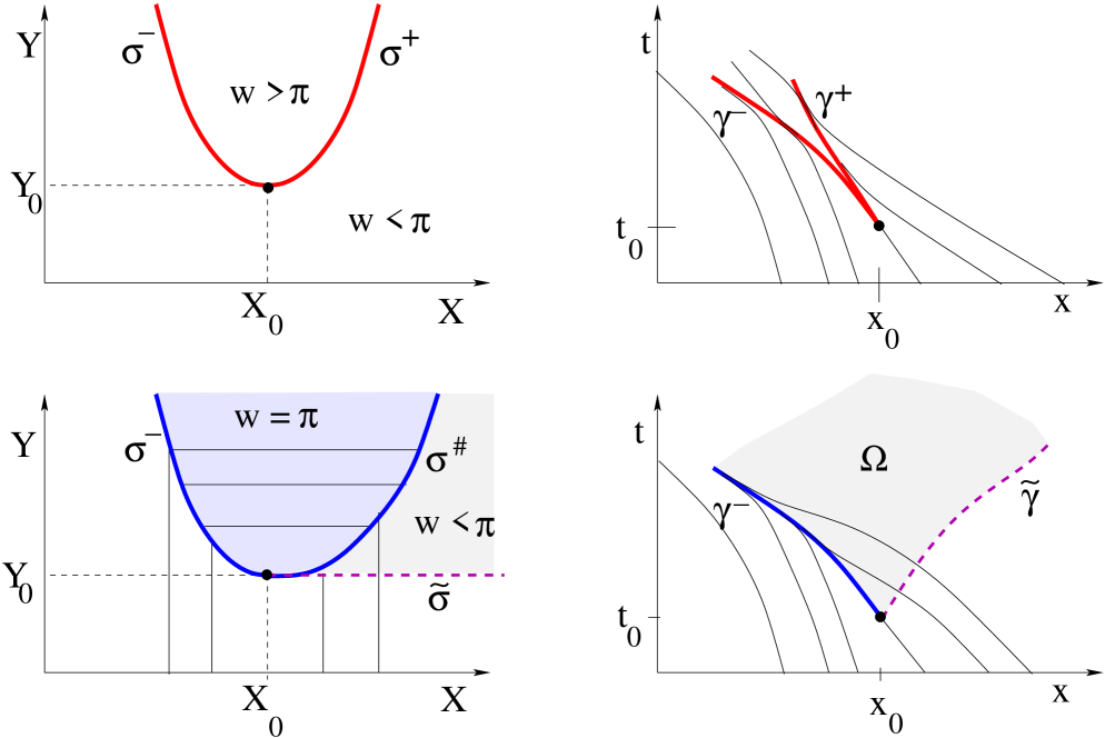
Figure 6: The positions of the singularities in the X 𝑋 X Y 𝑌 Y x 𝑥 x t 𝑡 t σ − superscript 𝜎 \sigma^{-} σ ♯ superscript 𝜎 ♯ \sigma^{\sharp} γ − superscript 𝛾 \gamma^{-} X 𝑋 X Y 𝑌 Y x 𝑥 x t 𝑡 t Ω Ω \Omega γ − superscript 𝛾 \gamma^{-} σ − superscript 𝜎 \sigma^{-} σ ♯ superscript 𝜎 ♯ \sigma^{\sharp} γ ~ ~ 𝛾 \tilde{\gamma} σ ~ ~ 𝜎 \tilde{\sigma}
Up to the time t 0 = t ( X 0 , Y 0 ) subscript 𝑡 0 𝑡 subscript 𝑋 0 subscript 𝑌 0 t_{0}=t(X_{0},Y_{0}) t > t 0 𝑡 subscript 𝑡 0 t>t_{0}
Ω ≐ { ( x , t ) ; t ≥ t 0 , γ − ( t ) ≤ x ≤ γ ~ ( t ) } , \Omega~{}\doteq~{}\bigl{\{}(x,t)\,;\qquad t\geq t_{0}\,,\quad\gamma^{-}(t)\leq x\leq\tilde{\gamma}(t)\bigr{\}}, (4.4)
where γ ~ ~ 𝛾 \tilde{\gamma} ( x 0 , t 0 ) subscript 𝑥 0 subscript 𝑡 0 (x_{0},t_{0}) 6 X 𝑋 X Y 𝑌 Y x 𝑥 x t 𝑡 t 7 t > t 0 𝑡 subscript 𝑡 0 t>t_{0} Theorem 4.
In the above setting,
the conservative solution u c o n s ( t , ⋅ ) superscript 𝑢 𝑐 𝑜 𝑛 𝑠 𝑡 ⋅ u^{cons}(t,\cdot) x = γ − ( t ) 𝑥 superscript 𝛾 𝑡 x=\gamma^{-}(t) x = γ + ( t ) 𝑥 superscript 𝛾 𝑡 x=\gamma^{+}(t) | u x c o n s | → ∞ → subscript superscript 𝑢 𝑐 𝑜 𝑛 𝑠 𝑥 |u^{cons}_{x}|\to\infty
On the other hand, the dissipative solution u d i s s ( t , ⋅ ) superscript 𝑢 𝑑 𝑖 𝑠 𝑠 𝑡 ⋅ u^{diss}(t,\cdot) x = γ − ( t ) 𝑥 superscript 𝛾 𝑡 x=\gamma^{-}(t) | u x d i s s | → ∞ → subscript superscript 𝑢 𝑑 𝑖 𝑠 𝑠 𝑥 |u^{diss}_{x}|\to\infty x = γ ~ ( t ) 𝑥 ~ 𝛾 𝑡 x=\tilde{\gamma}(t) u x d i s s subscript superscript 𝑢 𝑑 𝑖 𝑠 𝑠 𝑥 u^{diss}_{x} u x x d i s s subscript superscript 𝑢 𝑑 𝑖 𝑠 𝑠 𝑥 𝑥 u^{diss}_{xx}
The difference between these two solutions can be estimated as
∥ u c o n s ( t , ⋅ ) − u d i s s ( t , ⋅ ) ∥ 𝒞 0 ( ℝ ) = 𝒪 ( 1 ) ⋅ ( t − t 0 ) . \bigl{\|}u^{cons}(t,\cdot)-u^{diss}(t,\cdot)\|_{{\mathcal{C}}^{0}({\mathbb{R}})}~{}=~{}{\cal O}(1)\cdot(t-t_{0}). (4.5)
Figure 7: Comparing a conservative and a dissipative solution,
at a time t > t 0 𝑡 subscript 𝑡 0 t>t_{0} γ − ( t ) < γ + ( t ) superscript 𝛾 𝑡 superscript 𝛾 𝑡 \gamma^{-}(t)<\gamma^{+}(t) γ − ( t ) superscript 𝛾 𝑡 \gamma^{-}(t) γ ~ ( t ) ~ 𝛾 𝑡 \tilde{\gamma}(t) x ≤ γ − ( t ) 𝑥 superscript 𝛾 𝑡 x\leq\gamma^{-}(t) x ≥ γ ~ ( t ) 𝑥 ~ 𝛾 𝑡 x\geq\tilde{\gamma}(t)
Proof. 1. To fix the ideas,
assume that at the point P = ( X 0 , Y 0 ) 𝑃 subscript 𝑋 0 subscript 𝑌 0 P=(X_{0},Y_{0})
w X X < 0 , w Y > 0 , c ′ ( u ) > 0 . formulae-sequence subscript 𝑤 𝑋 𝑋 0 formulae-sequence subscript 𝑤 𝑌 0 superscript 𝑐 ′ 𝑢 0 w_{XX}~{}<~{}0,\qquad\qquad w_{Y}~{}>~{}0,\qquad\qquad c^{\prime}(u)~{}>~{}0.
In the X 𝑋 X Y 𝑌 Y ( x , t , u , w , z , p , q ) 𝑥 𝑡 𝑢 𝑤 𝑧 𝑝 𝑞 (x,t,u,w,z,p,q) 4.1 4.2 2. For X ≥ X 0 𝑋 subscript 𝑋 0 X\geq X_{0} Y = σ ♯ ( X ) 𝑌 superscript 𝜎 ♯ 𝑋 Y=\sigma^{\sharp}(X) w = π 𝑤 𝜋 w=\pi σ ♯ superscript 𝜎 ♯ \sigma^{\sharp}
w ( X , Y 0 ) = w 0 + w X X ( X 0 , Y 0 ) ⋅ ( X − X 0 ) 2 2 + 𝒪 ( 1 ) ⋅ ( X − X 0 ) 3 , 𝑤 𝑋 subscript 𝑌 0 subscript 𝑤 0 ⋅ subscript 𝑤 𝑋 𝑋 subscript 𝑋 0 subscript 𝑌 0 superscript 𝑋 subscript 𝑋 0 2 2 ⋅ 𝒪 1 superscript 𝑋 subscript 𝑋 0 3 w(X,Y_{0})~{}=~{}w_{0}+w_{XX}(X_{0},Y_{0})\cdot{(X-X_{0})^{2}\over 2}+{\cal O}(1)\cdot(X-X_{0})^{3},
w Y ( X , Y ) = w Y ( X 0 , Y 0 ) + 𝒪 ( 1 ) ⋅ ( | X − X 0 | + | Y − Y 0 | ) , subscript 𝑤 𝑌 𝑋 𝑌 subscript 𝑤 𝑌 subscript 𝑋 0 subscript 𝑌 0 ⋅ 𝒪 1 𝑋 subscript 𝑋 0 𝑌 subscript 𝑌 0 w_{Y}(X,Y)~{}=~{}w_{Y}(X_{0},Y_{0})+{\cal O}(1)\cdot\bigl{(}|X-X_{0}|+|Y-Y_{0}|\bigr{)},
valid in the region where w < π 𝑤 𝜋 w<\pi
σ ♯ ( X ) = Y 0 + κ ( X − X 0 ) 2 + 𝒪 ( 1 ) ⋅ ( X − X 0 ) 3 , superscript 𝜎 ♯ 𝑋 subscript 𝑌 0 𝜅 superscript 𝑋 subscript 𝑋 0 2 ⋅ 𝒪 1 superscript 𝑋 subscript 𝑋 0 3 \sigma^{\sharp}(X)~{}=~{}Y_{0}+\kappa(X-X_{0})^{2}+{\cal O}(1)\cdot(X-X_{0})^{3}, (4.6)
where κ > 0 𝜅 0 \kappa>0 3.37
For Y ′ > Y 0 superscript 𝑌 ′ subscript 𝑌 0 Y^{\prime}>Y_{0} 3.38 4.6
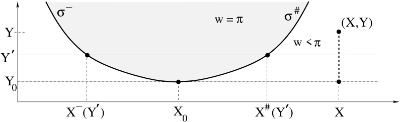
X ♯ ( Y ′ ) − X − ( Y ′ ) = 2 ( Y ′ − Y 0 κ ) 1 / 2 + 𝒪 ( 1 ) ⋅ | Y ′ − Y 0 | . superscript 𝑋 ♯ superscript 𝑌 ′ superscript 𝑋 superscript 𝑌 ′ 2 superscript superscript 𝑌 ′ subscript 𝑌 0 𝜅 1 2 ⋅ 𝒪 1 superscript 𝑌 ′ subscript 𝑌 0 X^{\sharp}(Y^{\prime})-X^{-}(Y^{\prime})~{}=~{}2\left({Y^{\prime}-Y_{0}\over\kappa}\right)^{1/2}+{\cal O}(1)\cdot|Y^{\prime}-Y_{0}|\,. (4.7)
Figure 8: Estimating the values of a dissipative solution
near a singularity. Notice that the functions
x , t , u 𝑥 𝑡 𝑢
x,t,u w = π 𝑤 𝜋 w=\pi
3. Consider a point ( X , Y ) 𝑋 𝑌 (X,Y) X > X 0 𝑋 subscript 𝑋 0 X>X_{0} Y ≤ σ ♯ ( X ) 𝑌 superscript 𝜎 ♯ 𝑋 Y\leq\sigma^{\sharp}(X) 2.9
u ( X , Y ) = u ( X , Y 0 ) + ∫ Y 0 Y ( sin z 4 c ( u ) q ) ( X , Y ′ ) 𝑑 Y ′ . 𝑢 𝑋 𝑌 𝑢 𝑋 subscript 𝑌 0 superscript subscript subscript 𝑌 0 𝑌 𝑧 4 𝑐 𝑢 𝑞 𝑋 superscript 𝑌 ′ differential-d superscript 𝑌 ′ u(X,Y)~{}=~{}u(X,Y_{0})+\int_{Y_{0}}^{Y}\left({\sin z\over 4c(u)}\,q\right)(X,Y^{\prime})\,dY^{\prime}\,. (4.8)
As in Fig. 8 Y ′ ∈ [ Y 0 , Y ] superscript 𝑌 ′ subscript 𝑌 0 𝑌 Y^{\prime}\in[Y_{0},Y] X − ( Y ′ ) superscript 𝑋 superscript 𝑌 ′ X^{-}(Y^{\prime}) X ♯ ( Y ′ ) superscript 𝑋 ♯ superscript 𝑌 ′ X^{\sharp}(Y^{\prime}) σ − ( X ) = Y ′ superscript 𝜎 𝑋 superscript 𝑌 ′ \sigma^{-}(X)=Y^{\prime} σ ♯ ( X ) = Y ′ superscript 𝜎 ♯ 𝑋 superscript 𝑌 ′ \sigma^{\sharp}(X)=Y^{\prime} z X = q X = 0 subscript 𝑧 𝑋 subscript 𝑞 𝑋 0 z_{X}=q_{X}=0 w = π 𝑤 𝜋 w=\pi 4.1 4.2
z ( X , Y ′ ) = z ( X − ( Y ′ ) , Y ′ ) + ∫ X − ( Y ′ ) X z X ( X ′ , Y ′ ) 𝑑 X ′ = z ( X − ( Y ′ ) , Y ′ ) + ∫ X ♯ ( Y ′ ) X ( c ′ ( u ) 8 c 2 ( u ) ( cos w − cos z ) p ) ( X ′ , Y ′ ) 𝑑 X ′ , 𝑧 𝑋 superscript 𝑌 ′ 𝑧 superscript 𝑋 superscript 𝑌 ′ superscript 𝑌 ′ superscript subscript superscript 𝑋 superscript 𝑌 ′ 𝑋 subscript 𝑧 𝑋 superscript 𝑋 ′ superscript 𝑌 ′ differential-d superscript 𝑋 ′ 𝑧 superscript 𝑋 superscript 𝑌 ′ superscript 𝑌 ′ superscript subscript superscript 𝑋 ♯ superscript 𝑌 ′ 𝑋 superscript 𝑐 ′ 𝑢 8 superscript 𝑐 2 𝑢 𝑤 𝑧 𝑝 superscript 𝑋 ′ superscript 𝑌 ′ differential-d superscript 𝑋 ′ \begin{split}z(X,Y^{\prime})~{}&=~{}z(X^{-}(Y^{\prime}),Y^{\prime})+\int_{X^{-}(Y^{\prime})}^{X}z_{X}(X^{\prime},Y^{\prime})\,dX^{\prime}\\
&~{}=~{}z(X^{-}(Y^{\prime}),Y^{\prime})+\int_{X^{\sharp}(Y^{\prime})}^{X}\left({c^{\prime}(u)\over 8c^{2}(u)}\,(\cos w-\cos z)\,p\right)(X^{\prime},Y^{\prime})\,dX^{\prime},\end{split} (4.9)
q ( X , Y ′ ) = q ( X − ( Y ′ ) , Y ′ ) + ∫ X ♯ ( Y ′ ) X ( c ′ ( u ) 8 c 2 ( u ) [ sin w − sin z ] p q ) ( X ′ , Y ′ ) 𝑑 X ′ . 𝑞 𝑋 superscript 𝑌 ′ 𝑞 superscript 𝑋 superscript 𝑌 ′ superscript 𝑌 ′ superscript subscript superscript 𝑋 ♯ superscript 𝑌 ′ 𝑋 superscript 𝑐 ′ 𝑢 8 superscript 𝑐 2 𝑢 delimited-[] 𝑤 𝑧 𝑝 𝑞 superscript 𝑋 ′ superscript 𝑌 ′ differential-d superscript 𝑋 ′ q(X,Y^{\prime})~{}=~{}q(X^{-}(Y^{\prime}),Y^{\prime})+\int_{X^{\sharp}(Y^{\prime})}^{X}\left({c^{\prime}(u)\over 8c^{2}(u)}\,\big{[}\sin w-\sin z\big{]}\,pq\right)(X^{\prime},Y^{\prime})\,dX^{\prime}. (4.10)
4.
For notational convenience, in the following we denote by
( x , t , u , w , z , p , q ) ( X , Y ) 𝑥 𝑡 𝑢 𝑤 𝑧 𝑝 𝑞 𝑋 𝑌 (x,t,u,w,z,p,q)(X,Y) ( x ^ , t ^ , u ^ , w ^ , z ^ , p ^ , q ^ ) ( X , Y ) ^ 𝑥 ^ 𝑡 ^ 𝑢 ^ 𝑤 ^ 𝑧 ^ 𝑝 ^ 𝑞 𝑋 𝑌 (\hat{x},\hat{t},\hat{u},\hat{w},\hat{z},\hat{p},\hat{q})(X,Y) 6 ( X , Y ) 𝑋 𝑌 (X,Y) σ − superscript 𝜎 \sigma^{-} σ ~ ~ 𝜎 \tilde{\sigma}
{ X ≤ X 0 , Y > σ − ( X ) } ∪ { X ≥ X 0 , Y > Y 0 } . formulae-sequence 𝑋 subscript 𝑋 0 𝑌 superscript 𝜎 𝑋 formulae-sequence 𝑋 subscript 𝑋 0 𝑌 subscript 𝑌 0 \bigl{\{}X\leq X_{0}\,,\quad Y>\sigma^{-}(X)\bigr{\}}~{}\cup~{}\bigl{\{}X\geq X_{0}\,,\quad Y>Y_{0}\bigr{\}}.
Consider a point ( X , Y ′ ) 𝑋 superscript 𝑌 ′ (X,Y^{\prime}) X > X 0 𝑋 subscript 𝑋 0 X>X_{0} Y ′ < σ ♯ ( X ) superscript 𝑌 ′ superscript 𝜎 ♯ 𝑋 Y^{\prime}<\sigma^{\sharp}(X) 4.1 z = z ^ 𝑧 ^ 𝑧 z=\hat{z} Y ≤ Y 0 𝑌 subscript 𝑌 0 Y\leq Y_{0} 4.7
z ^ ( X , Y ′ ) − z ( X , Y ′ ) = ∫ X − ( Y ′ ) X ♯ ( Y ′ ) z ^ X ( X ′ , Y ′ ) 𝑑 X ′ + ∫ X ♯ ( Y ′ ) X ( z ^ X − z X ) ( X ′ , Y ′ ) 𝑑 X ′ = − c ′ ( u 0 ) ( 1 + cos z 0 ) 8 c 2 ( u 0 ) p 0 ⋅ ( X ♯ ( Y ′ ) − X − ( Y ′ ) ) + 𝒪 ( 1 ) ⋅ ( X ♯ ( Y ′ ) − X − ( Y ′ ) ) 2 + 𝒪 ( 1 ) ⋅ ( X − X ♯ ( Y ′ ) ) ( Y ′ − Y 0 ) = − c ′ ( u 0 ) ( 1 + cos z 0 ) 4 c 2 ( u 0 ) κ 1 / 2 p 0 ⋅ ( Y ′ − Y 0 ) 1 / 2 + 𝒪 ( 1 ) ⋅ | Y ′ − Y 0 | . ^ 𝑧 𝑋 superscript 𝑌 ′ 𝑧 𝑋 superscript 𝑌 ′ missing-subexpression absent superscript subscript superscript 𝑋 superscript 𝑌 ′ superscript 𝑋 ♯ superscript 𝑌 ′ subscript ^ 𝑧 𝑋 superscript 𝑋 ′ superscript 𝑌 ′ differential-d superscript 𝑋 ′ superscript subscript superscript 𝑋 ♯ superscript 𝑌 ′ 𝑋 subscript ^ 𝑧 𝑋 subscript 𝑧 𝑋 superscript 𝑋 ′ superscript 𝑌 ′ differential-d superscript 𝑋 ′ missing-subexpression absent ⋅ superscript 𝑐 ′ subscript 𝑢 0 1 subscript 𝑧 0 8 superscript 𝑐 2 subscript 𝑢 0 subscript 𝑝 0 superscript 𝑋 ♯ superscript 𝑌 ′ superscript 𝑋 superscript 𝑌 ′ missing-subexpression ⋅ 𝒪 1 superscript superscript 𝑋 ♯ superscript 𝑌 ′ superscript 𝑋 superscript 𝑌 ′ 2 ⋅ 𝒪 1 𝑋 superscript 𝑋 ♯ superscript 𝑌 ′ superscript 𝑌 ′ subscript 𝑌 0 missing-subexpression absent ⋅ superscript 𝑐 ′ subscript 𝑢 0 1 subscript 𝑧 0 4 superscript 𝑐 2 subscript 𝑢 0 superscript 𝜅 1 2 subscript 𝑝 0 superscript superscript 𝑌 ′ subscript 𝑌 0 1 2 ⋅ 𝒪 1 superscript 𝑌 ′ subscript 𝑌 0 \begin{array}[]{l}\hat{z}(X,Y^{\prime})-z(X,Y^{\prime})\cr\cr\quad\displaystyle=~{}\int_{X^{-}(Y^{\prime})}^{X^{\sharp}(Y^{\prime})}\hat{z}_{X}(X^{\prime},Y^{\prime})\,dX^{\prime}+\int_{X^{\sharp}(Y^{\prime})}^{X}\left(\hat{z}_{X}-z_{X}\right)(X^{\prime},Y^{\prime})\,dX^{\prime}\cr\cr\quad=~{}\displaystyle-{c^{\prime}(u_{0})(1+\cos z_{0})\over 8c^{2}(u_{0})}\,p_{0}\cdot\bigl{(}X^{\sharp}(Y^{\prime})-X^{-}(Y^{\prime})\bigr{)}\cr\cr\qquad\displaystyle+{\cal O}(1)\cdot\bigl{(}X^{\sharp}(Y^{\prime})-X^{-}(Y^{\prime})\bigr{)}^{2}+{\cal O}(1)\cdot\bigl{(}X-X^{\sharp}(Y^{\prime})\bigr{)}\,(Y^{\prime}-Y_{0})\cr\cr\quad=~{}\displaystyle-{c^{\prime}(u_{0})(1+\cos z_{0})\over 4c^{2}(u_{0})\,\kappa^{1/2}}\,p_{0}\cdot(Y^{\prime}-Y_{0})^{1/2}+{\cal O}(1)\cdot|Y^{\prime}-Y_{0}|\,.\end{array} (4.11)
By (4.2
q ^ ( X , Y ′ ) − q ( X , Y ′ ) = ∫ X − ( Y ′ ) X ♯ ( Y ′ ) q ^ X ( X ′ , Y ′ ) 𝑑 X ′ + ∫ X ♯ ( Y ′ ) X ( q ^ X − q X ) ( X ′ , Y ′ ) 𝑑 X ′ = − c ′ ( u 0 ) sin z 0 8 c 2 ( u 0 ) p 0 q 0 ⋅ ( X ♯ ( Y ′ ) − X − ( Y ′ ) ) + 𝒪 ( 1 ) ⋅ ( X ♯ ( Y ′ ) − X − ( Y ′ ) ) 2 + 𝒪 ( 1 ) ⋅ ( X − X ♯ ( Y ′ ) ) ( Y ′ − Y 0 ) = − c ′ ( u 0 ) sin z 0 4 c 2 ( u 0 ) κ 1 / 2 p 0 q 0 ⋅ ( Y ′ − Y 0 ) 1 / 2 + 𝒪 ( 1 ) ⋅ | Y ′ − Y 0 | . ^ 𝑞 𝑋 superscript 𝑌 ′ 𝑞 𝑋 superscript 𝑌 ′ missing-subexpression absent superscript subscript superscript 𝑋 superscript 𝑌 ′ superscript 𝑋 ♯ superscript 𝑌 ′ subscript ^ 𝑞 𝑋 superscript 𝑋 ′ superscript 𝑌 ′ differential-d superscript 𝑋 ′ superscript subscript superscript 𝑋 ♯ superscript 𝑌 ′ 𝑋 subscript ^ 𝑞 𝑋 subscript 𝑞 𝑋 superscript 𝑋 ′ superscript 𝑌 ′ differential-d superscript 𝑋 ′ missing-subexpression absent ⋅ superscript 𝑐 ′ subscript 𝑢 0 subscript 𝑧 0 8 superscript 𝑐 2 subscript 𝑢 0 subscript 𝑝 0 subscript 𝑞 0 superscript 𝑋 ♯ superscript 𝑌 ′ superscript 𝑋 superscript 𝑌 ′ missing-subexpression ⋅ 𝒪 1 superscript superscript 𝑋 ♯ superscript 𝑌 ′ superscript 𝑋 superscript 𝑌 ′ 2 ⋅ 𝒪 1 𝑋 superscript 𝑋 ♯ superscript 𝑌 ′ superscript 𝑌 ′ subscript 𝑌 0 missing-subexpression absent ⋅ superscript 𝑐 ′ subscript 𝑢 0 subscript 𝑧 0 4 superscript 𝑐 2 subscript 𝑢 0 superscript 𝜅 1 2 subscript 𝑝 0 subscript 𝑞 0 superscript superscript 𝑌 ′ subscript 𝑌 0 1 2 ⋅ 𝒪 1 superscript 𝑌 ′ subscript 𝑌 0 \begin{array}[]{l}\hat{q}(X,Y^{\prime})-q(X,Y^{\prime})\cr\cr\quad\displaystyle=~{}\int_{X^{-}(Y^{\prime})}^{X^{\sharp}(Y^{\prime})}\hat{q}_{X}(X^{\prime},Y^{\prime})\,dX^{\prime}+\int_{X^{\sharp}(Y^{\prime})}^{X}\left(\hat{q}_{X}-q_{X}\right)(X^{\prime},Y^{\prime})\,dX^{\prime}\cr\cr\quad=~{}\displaystyle-{c^{\prime}(u_{0})\sin z_{0}\over 8c^{2}(u_{0})}\,p_{0}q_{0}\cdot\bigl{(}X^{\sharp}(Y^{\prime})-X^{-}(Y^{\prime})\bigr{)}\cr\cr\qquad\displaystyle+{\cal O}(1)\cdot\bigl{(}X^{\sharp}(Y^{\prime})-X^{-}(Y^{\prime})\bigr{)}^{2}+{\cal O}(1)\cdot\bigl{(}X-X^{\sharp}(Y^{\prime})\bigr{)}\,(Y^{\prime}-Y_{0})\cr\cr\quad=~{}\displaystyle-{c^{\prime}(u_{0})\sin z_{0}\over 4c^{2}(u_{0})\,\kappa^{1/2}}\,p_{0}q_{0}\cdot(Y^{\prime}-Y_{0})^{1/2}+{\cal O}(1)\cdot|Y^{\prime}-Y_{0}|\,.\end{array} (4.12)
Next, using the second equation in (2.9 u ( X , Y 0 ) = u ^ ( X , Y 0 ) 𝑢 𝑋 subscript 𝑌 0 ^ 𝑢 𝑋 subscript 𝑌 0 u(X,Y_{0})=\hat{u}(X,Y_{0}) X ∈ [ X 0 , X 0 + 1 ] 𝑋 subscript 𝑋 0 subscript 𝑋 0 1 X\in[X_{0},\,X_{0}+1] Y ∈ [ Y 0 , σ ♯ ( X ) ] 𝑌 subscript 𝑌 0 superscript 𝜎 ♯ 𝑋 Y\in[Y_{0},\sigma^{\sharp}(X)]
u ^ ( X , Y ) − u ( X , Y ) = ∫ Y 0 Y ( sin z ^ 4 c ( u ^ ) q ^ − sin z 4 c ( u ) q ) ( X , Y ′ ) 𝑑 Y ′ = ∫ Y 0 Y ( cos z 0 4 c ( u 0 ) q 0 ⋅ ( z ^ − z ) + sin z 0 4 c ( u 0 ) ⋅ ( q ^ − q ) − c ′ ( u 0 ) sin z 0 4 c 2 ( u 0 ) q 0 ⋅ ( u ^ − u ) ) ( X , Y ′ ) 𝑑 Y ′ + 𝒪 ( 1 ) ⋅ ∫ Y 0 Y ( | z ^ − z | 2 + | q ^ − q | 2 + | u ^ − u | 2 ) ( X , Y ′ ) 𝑑 Y ′ + 𝒪 ( 1 ) ⋅ ( | X − X 0 | + | Y − Y 0 | ) ⋅ ∫ Y 0 Y ( | z ^ − z | + | q ^ − q | + | u ^ − u | ) ( X , Y ′ ) 𝑑 Y ′ = η 0 ⋅ ( Y − Y 0 ) 3 / 2 + 𝒪 ( 1 ) ⋅ | Y − Y 0 | 2 , ^ 𝑢 𝑋 𝑌 𝑢 𝑋 𝑌 superscript subscript subscript 𝑌 0 𝑌 ^ 𝑧 4 𝑐 ^ 𝑢 ^ 𝑞 𝑧 4 𝑐 𝑢 𝑞 𝑋 superscript 𝑌 ′ differential-d superscript 𝑌 ′ missing-subexpression absent superscript subscript subscript 𝑌 0 𝑌 ⋅ subscript 𝑧 0 4 𝑐 subscript 𝑢 0 subscript 𝑞 0 ^ 𝑧 𝑧 ⋅ subscript 𝑧 0 4 𝑐 subscript 𝑢 0 ^ 𝑞 𝑞 ⋅ superscript 𝑐 ′ subscript 𝑢 0 subscript 𝑧 0 4 superscript 𝑐 2 subscript 𝑢 0 subscript 𝑞 0 ^ 𝑢 𝑢 𝑋 superscript 𝑌 ′ differential-d superscript 𝑌 ′ missing-subexpression ⋅ 𝒪 1 superscript subscript subscript 𝑌 0 𝑌 superscript ^ 𝑧 𝑧 2 superscript ^ 𝑞 𝑞 2 superscript ^ 𝑢 𝑢 2 𝑋 superscript 𝑌 ′ differential-d superscript 𝑌 ′ missing-subexpression ⋅ 𝒪 1 𝑋 subscript 𝑋 0 𝑌 subscript 𝑌 0 superscript subscript subscript 𝑌 0 𝑌 ^ 𝑧 𝑧 ^ 𝑞 𝑞 ^ 𝑢 𝑢 𝑋 superscript 𝑌 ′ differential-d superscript 𝑌 ′ missing-subexpression absent ⋅ subscript 𝜂 0 superscript 𝑌 subscript 𝑌 0 3 2 ⋅ 𝒪 1 superscript 𝑌 subscript 𝑌 0 2 \begin{array}[]{l}\displaystyle\hat{u}(X,Y)-u(X,Y)~{}=~{}\int_{Y_{0}}^{Y}\left({\sin\hat{z}\over 4c(\hat{u})}\,\hat{q}-{\sin z\over 4c(u)}\,q\right)(X,Y^{\prime})\,dY^{\prime}\cr\cr\displaystyle\qquad=~{}\int_{Y_{0}}^{Y}\left({\cos z_{0}\over 4c(u_{0})}\,q_{0}\cdot(\hat{z}-z)+{\sin z_{0}\over 4c(u_{0})}\,\cdot(\hat{q}-q)-{c^{\prime}(u_{0})\sin z_{0}\over 4c^{2}(u_{0})}\,q_{0}\cdot(\hat{u}-u)\right)(X,Y^{\prime})\,dY^{\prime}\cr\cr\qquad\qquad\displaystyle+{\cal O}(1)\cdot\int_{Y_{0}}^{Y}\Big{(}|\hat{z}-z|^{2}+|\hat{q}-q|^{2}+|\hat{u}-u|^{2}\Big{)}(X,Y^{\prime})\,dY^{\prime}\cr\cr\qquad\qquad\displaystyle+{\cal O}(1)\cdot\Big{(}|X-X_{0}|+|Y-Y_{0}|\Big{)}\cdot\int_{Y_{0}}^{Y}\Big{(}|\hat{z}-z|+|\hat{q}-q|+|\hat{u}-u|\Big{)}(X,Y^{\prime})\,dY^{\prime}\cr\cr\qquad=~{}\eta_{0}\cdot(Y-Y_{0})^{3/2}+{\cal O}(1)\cdot|Y-Y_{0}|^{2},\end{array} (4.13)
where the constant η 0 subscript 𝜂 0 \eta_{0}
η 0 = 2 3 [ − c ′ ( u 0 ) ( 1 + cos z 0 ) 4 c 2 ( u 0 ) κ 1 / 2 p 0 ] ⋅ cos z 0 4 c ( u 0 ) q 0 + 2 3 [ − c ′ ( u 0 ) sin z 0 4 c 2 ( u 0 ) κ 1 / 2 p 0 q 0 ] ⋅ sin z 0 4 c ( u 0 ) . subscript 𝜂 0 ⋅ 2 3 delimited-[] superscript 𝑐 ′ subscript 𝑢 0 1 subscript 𝑧 0 4 superscript 𝑐 2 subscript 𝑢 0 superscript 𝜅 1 2 subscript 𝑝 0 subscript 𝑧 0 4 𝑐 subscript 𝑢 0 subscript 𝑞 0 ⋅ 2 3 delimited-[] superscript 𝑐 ′ subscript 𝑢 0 subscript 𝑧 0 4 superscript 𝑐 2 subscript 𝑢 0 superscript 𝜅 1 2 subscript 𝑝 0 subscript 𝑞 0 subscript 𝑧 0 4 𝑐 subscript 𝑢 0 \eta_{0}~{}=~{}{2\over 3}\left[-{c^{\prime}(u_{0})(1+\cos z_{0})\over 4c^{2}(u_{0})\,\kappa^{1/2}}\,p_{0}\right]\cdot{\cos z_{0}\over 4c(u_{0})}\,q_{0}+{2\over 3}\left[-{c^{\prime}(u_{0})\,\sin z_{0}\over 4c^{2}(u_{0})\,\kappa^{1/2}}\,p_{0}q_{0}\right]\cdot{\sin z_{0}\over 4c(u_{0})}\,. (4.14)
5. Using the second equations in (2.12 2.13 x , t 𝑥 𝑡
x,t
x ^ ( X , Y ) − x ( X , Y ) = − ∫ Y 0 Y ( 1 + cos z ^ 4 q ^ − 1 + cos z 4 q ) ( X , Y ′ ) 𝑑 Y ′ = ∫ Y 0 Y ( sin z 0 4 q 0 ⋅ ( z ^ − z ) − 1 + cos z 0 4 ⋅ ( q ^ − q ) ) ( X , Y ′ ) 𝑑 Y ′ + 𝒪 ( 1 ) ⋅ ∫ Y 0 Y ( | z ^ − z | 2 + | q ^ − q | 2 ) ( X , Y ′ ) 𝑑 Y ′ + 𝒪 ( 1 ) ⋅ ( | X − X 0 | + | Y − Y 0 | ) ⋅ ∫ Y 0 Y ( | z ^ − z | + | q ^ − q | ) ( X , Y ′ ) 𝑑 Y ′ = 𝒪 ( 1 ) ⋅ | Y − Y 0 | 2 . ^ 𝑥 𝑋 𝑌 𝑥 𝑋 𝑌 superscript subscript subscript 𝑌 0 𝑌 1 ^ 𝑧 4 ^ 𝑞 1 𝑧 4 𝑞 𝑋 superscript 𝑌 ′ differential-d superscript 𝑌 ′ missing-subexpression absent superscript subscript subscript 𝑌 0 𝑌 ⋅ subscript 𝑧 0 4 subscript 𝑞 0 ^ 𝑧 𝑧 ⋅ 1 subscript 𝑧 0 4 ^ 𝑞 𝑞 𝑋 superscript 𝑌 ′ differential-d superscript 𝑌 ′ missing-subexpression ⋅ 𝒪 1 superscript subscript subscript 𝑌 0 𝑌 superscript ^ 𝑧 𝑧 2 superscript ^ 𝑞 𝑞 2 𝑋 superscript 𝑌 ′ differential-d superscript 𝑌 ′ missing-subexpression ⋅ 𝒪 1 𝑋 subscript 𝑋 0 𝑌 subscript 𝑌 0 superscript subscript subscript 𝑌 0 𝑌 ^ 𝑧 𝑧 ^ 𝑞 𝑞 𝑋 superscript 𝑌 ′ differential-d superscript 𝑌 ′ missing-subexpression absent ⋅ 𝒪 1 superscript 𝑌 subscript 𝑌 0 2 \begin{array}[]{l}\displaystyle\hat{x}(X,Y)-x(X,Y)~{}=~{}-\int_{Y_{0}}^{Y}\left({1+\cos\hat{z}\over 4}\,\hat{q}-{1+\cos z\over 4}\,q\right)(X,Y^{\prime})\,dY^{\prime}\cr\cr\displaystyle\qquad=~{}\int_{Y_{0}}^{Y}\left({\sin z_{0}\over 4}\,q_{0}\cdot(\hat{z}-z)-{1+\cos z_{0}\over 4}\,\cdot(\hat{q}-q)\right)(X,Y^{\prime})\,dY^{\prime}\cr\cr\qquad\qquad\displaystyle+{\cal O}(1)\cdot\int_{Y_{0}}^{Y}\Big{(}|\hat{z}-z|^{2}+|\hat{q}-q|^{2}\Big{)}(X,Y^{\prime})\,dY^{\prime}\cr\cr\qquad\qquad\displaystyle+{\cal O}(1)\cdot\Big{(}|X-X_{0}|+|Y-Y_{0}|\Big{)}\cdot\int_{Y_{0}}^{Y}\Big{(}|\hat{z}-z|+|\hat{q}-q|\Big{)}(X,Y^{\prime})\,dY^{\prime}\cr\cr\qquad=~{}{\cal O}(1)\cdot|Y-Y_{0}|^{2}.\end{array} (4.15)
Indeed, the coefficient of the leading order term 𝒪 ( 1 ) ⋅ ( Y − Y 0 ) 3 / 2 ⋅ 𝒪 1 superscript 𝑌 subscript 𝑌 0 3 2 {\cal O}(1)\cdot(Y-Y_{0})^{3/2}
t ^ ( X , Y ) − t ( X , Y ) = − ∫ Y 0 Y ( 1 + cos z ^ 4 c ( u ^ ) q ^ − 1 + cos z 4 c ( u ) q ) ( X , Y ′ ) 𝑑 Y ′ = ∫ Y 0 Y ( sin z 0 4 c ( u 0 ) q 0 ⋅ ( z ^ − z ) − 1 + cos z 0 4 c ( u 0 ) ⋅ ( q ^ − q ) + 1 + cos z 0 4 c 2 ( u 0 ) c ′ ( u 0 ) q 0 ⋅ ( u ^ − u ) ) ( X , Y ′ ) 𝑑 Y ′ + 𝒪 ( 1 ) ⋅ ∫ Y 0 Y ( | z ^ − z | 2 + | q ^ − q | 2 + | u ^ − u | 2 ) ( X , Y ′ ) 𝑑 Y ′ + 𝒪 ( 1 ) ⋅ ( | X − X 0 | + | Y − Y 0 | ) ⋅ ∫ Y 0 Y ( | z ^ − z | + | q ^ − q | + | u ^ − u | ) ( X , Y ′ ) 𝑑 Y ′ = 𝒪 ( 1 ) ⋅ | Y − Y 0 | 2 . ^ 𝑡 𝑋 𝑌 𝑡 𝑋 𝑌 superscript subscript subscript 𝑌 0 𝑌 1 ^ 𝑧 4 𝑐 ^ 𝑢 ^ 𝑞 1 𝑧 4 𝑐 𝑢 𝑞 𝑋 superscript 𝑌 ′ differential-d superscript 𝑌 ′ missing-subexpression absent superscript subscript subscript 𝑌 0 𝑌 ⋅ subscript 𝑧 0 4 𝑐 subscript 𝑢 0 subscript 𝑞 0 ^ 𝑧 𝑧 ⋅ 1 subscript 𝑧 0 4 𝑐 subscript 𝑢 0 ^ 𝑞 𝑞 ⋅ 1 subscript 𝑧 0 4 superscript 𝑐 2 subscript 𝑢 0 superscript 𝑐 ′ subscript 𝑢 0 subscript 𝑞 0 ^ 𝑢 𝑢 𝑋 superscript 𝑌 ′ differential-d superscript 𝑌 ′ missing-subexpression ⋅ 𝒪 1 superscript subscript subscript 𝑌 0 𝑌 superscript ^ 𝑧 𝑧 2 superscript ^ 𝑞 𝑞 2 superscript ^ 𝑢 𝑢 2 𝑋 superscript 𝑌 ′ differential-d superscript 𝑌 ′ missing-subexpression ⋅ 𝒪 1 𝑋 subscript 𝑋 0 𝑌 subscript 𝑌 0 superscript subscript subscript 𝑌 0 𝑌 ^ 𝑧 𝑧 ^ 𝑞 𝑞 ^ 𝑢 𝑢 𝑋 superscript 𝑌 ′ differential-d superscript 𝑌 ′ missing-subexpression absent ⋅ 𝒪 1 superscript 𝑌 subscript 𝑌 0 2 \begin{array}[]{l}\displaystyle\hat{t}(X,Y)-t(X,Y)~{}=~{}-\int_{Y_{0}}^{Y}\left({1+\cos\hat{z}\over 4c(\hat{u})}\,\hat{q}-{1+\cos z\over 4c(u)}\,q\right)(X,Y^{\prime})\,dY^{\prime}\cr\cr\displaystyle=~{}\int_{Y_{0}}^{Y}\left({\sin z_{0}\over 4c(u_{0})}\,q_{0}\cdot(\hat{z}-z)-{1+\cos z_{0}\over 4c(u_{0})}\,\cdot(\hat{q}-q)+{1+\cos z_{0}\over 4c^{2}(u_{0})}c^{\prime}(u_{0})q_{0}\cdot(\hat{u}-u)\right)(X,Y^{\prime})\,dY^{\prime}\cr\cr\qquad\qquad\displaystyle+{\cal O}(1)\cdot\int_{Y_{0}}^{Y}\Big{(}|\hat{z}-z|^{2}+|\hat{q}-q|^{2}+|\hat{u}-u|^{2}\Big{)}(X,Y^{\prime})\,dY^{\prime}\cr\cr\qquad\qquad\displaystyle+{\cal O}(1)\cdot\Big{(}|X-X_{0}|+|Y-Y_{0}|\Big{)}\cdot\int_{Y_{0}}^{Y}\Big{(}|\hat{z}-z|+|\hat{q}-q|+|\hat{u}-u|\Big{)}(X,Y^{\prime})\,dY^{\prime}\cr\cr=~{}{\cal O}(1)\cdot|Y-Y_{0}|^{2}.\end{array} (4.16)
6. The estimate (4.13 u ^ − u ^ 𝑢 𝑢 \hat{u}-u ( X , Y ) 𝑋 𝑌 (X,Y) u ^ − u ^ 𝑢 𝑢 \hat{u}-u x , t 𝑥 𝑡
x,t u 𝑢 u
P = ( x , t ) = ( x ( X , Y ) , t ( X , Y ) ) , 𝑃 𝑥 𝑡 𝑥 𝑋 𝑌 𝑡 𝑋 𝑌 P~{}=~{}(x,t)~{}=~{}\bigl{(}x(X,Y),\,t(X,Y)\bigr{)}, (4.17)
with
X > X 0 , Y 0 < Y < σ ♯ ( X ) . formulae-sequence 𝑋 subscript 𝑋 0 subscript 𝑌 0 𝑌 superscript 𝜎 ♯ 𝑋 X~{}>~{}X_{0},\qquad\qquad Y_{0}~{}<~{}Y~{}<~{}\sigma^{\sharp}(X). (4.18)
Moreover, let u ^ ^ 𝑢 \hat{u} ( X ^ , Y ^ ) ^ 𝑋 ^ 𝑌 (\widehat{X},\widehat{Y}) P 𝑃 P
P = ( x , t ) = ( x ^ ( X ^ , Y ^ ) , t ^ ( X ^ , Y ^ ) ) . 𝑃 𝑥 𝑡 ^ 𝑥 ^ 𝑋 ^ 𝑌 ^ 𝑡 ^ 𝑋 ^ 𝑌 P~{}=~{}(x,t)~{}=~{}\bigl{(}\hat{x}(\widehat{X},\,\widehat{Y}),\hat{t}(\widehat{X},\widehat{Y})\bigr{)}. (4.19)
Using (4.13 4.15 4.16 u ^ = u ^ ( x , t ) ^ 𝑢 ^ 𝑢 𝑥 𝑡 \hat{u}=\hat{u}(x,t) 1 / 2 1 2 1/2 x , t 𝑥 𝑡
x,t
| u ^ ( x , t ) − u ( x , t ) | ≤ | u ^ ( X ^ , Y ^ ) − u ^ ( X , Y ) | + | u ^ ( X , Y ) − u ( X , Y ) | = 𝒪 ( 1 ) ⋅ ( | x ^ ( X ^ , Y ^ ) − x ^ ( X , Y ) | 1 / 2 + | t ^ ( X ^ , Y ^ ) − t ^ ( X , Y ) | 1 / 2 ) + 𝒪 ( 1 ) ⋅ | Y − Y 0 | 3 / 2 = 𝒪 ( 1 ) ⋅ ( | x ( X , Y ) − x ^ ( X , Y ) | 1 / 2 + | t ( X , Y ) − t ^ ( X , Y ) | 1 / 2 ) + 𝒪 ( 1 ) ⋅ | Y − Y 0 | 3 / 2 = 𝒪 ( 1 ) ⋅ | Y − Y 0 | . \begin{array}[]{l}|\hat{u}(x,t)-u(x,t)|~{}\leq~{}\bigl{|}\hat{u}(\widehat{X},\widehat{Y})-\hat{u}(X,Y)\bigr{|}+\bigl{|}\hat{u}(X,Y)-u(X,Y)\bigr{|}\\[11.38109pt]
\qquad=~{}{\cal O}(1)\cdot\Big{(}\bigl{|}\hat{x}(\widehat{X},\widehat{Y})-\hat{x}(X,Y)\bigr{|}^{1/2}+\bigl{|}\hat{t}(\widehat{X},\widehat{Y})-\hat{t}(X,Y)\bigr{|}^{1/2}\Big{)}+{\cal O}(1)\cdot|Y-Y_{0}|^{3/2}\\[11.38109pt]
\qquad=~{}{\cal O}(1)\cdot\Big{(}\bigl{|}x(X,Y)-\hat{x}(X,Y)\bigr{|}^{1/2}+\bigl{|}t(X,Y)-\hat{t}(X,Y)\bigr{|}^{1/2}\Big{)}+{\cal O}(1)\cdot|Y-Y_{0}|^{3/2}\\[11.38109pt]
\qquad=~{}{\cal O}(1)\cdot|Y-Y_{0}|.\end{array} (4.20)
In a neighborhood of ( x 0 , t 0 ) subscript 𝑥 0 subscript 𝑡 0 (x_{0},t_{0})
t Y = 1 + cos z 4 c ( u ) q > 1 + cos z 0 5 c ( u 0 ) q 0 > 0 . subscript 𝑡 𝑌 1 𝑧 4 𝑐 𝑢 𝑞 1 subscript 𝑧 0 5 𝑐 subscript 𝑢 0 subscript 𝑞 0 0 t_{Y}~{}=~{}{1+\cos z\over 4c(u)}\,q~{}>~{}{1+\cos z_{0}\over 5c(u_{0})}q_{0}~{}>0\,. (4.21)
For ( x , t ) 𝑥 𝑡 (x,t) 4.17 4.18
t − t 0 = [ t ( X , Y ) − t ( X , Y 0 ) ] + [ t ( X , Y 0 ) − t ( X 0 , Y 0 ) ] ≥ 1 + cos z 0 5 c ( u 0 ) q 0 ⋅ | Y − Y 0 | . 𝑡 subscript 𝑡 0 delimited-[] 𝑡 𝑋 𝑌 𝑡 𝑋 subscript 𝑌 0 delimited-[] 𝑡 𝑋 subscript 𝑌 0 𝑡 subscript 𝑋 0 subscript 𝑌 0 ⋅ 1 subscript 𝑧 0 5 𝑐 subscript 𝑢 0 subscript 𝑞 0 𝑌 subscript 𝑌 0 t-t_{0}~{}=~{}\bigl{[}t(X,Y)-t(X,Y_{0})\bigr{]}+\bigl{[}t(X,Y_{0})-t(X_{0},Y_{0})\bigr{]}~{}\geq~{}{1+\cos z_{0}\over 5c(u_{0})}q_{0}\cdot|Y-Y_{0}|\,.
Together with (4.20 4.5 7. It remains to prove that the solution u = u ( t , x ) 𝑢 𝑢 𝑡 𝑥 u=u(t,x) γ ~ ~ 𝛾 \tilde{\gamma}
Consider a point ( x 1 , t 1 ) = ( x ( X , Y 0 ) , t ( X , Y 0 ) ) subscript 𝑥 1 subscript 𝑡 1 𝑥 𝑋 subscript 𝑌 0 𝑡 𝑋 subscript 𝑌 0 (x_{1},t_{1})=\bigl{(}x(X,Y_{0}),t(X,Y_{0})\bigr{)} γ ~ ~ 𝛾 \tilde{\gamma} X > X 0 𝑋 subscript 𝑋 0 X>X_{0} x = γ ( t ) 𝑥 𝛾 𝑡 x=\gamma(t) ( x 1 , t 1 ) subscript 𝑥 1 subscript 𝑡 1 (x_{1},t_{1})
γ ( t 1 ) = x 1 , γ ˙ ( t ) = c ( u ( γ ( t ) , t ) ) . formulae-sequence 𝛾 subscript 𝑡 1 subscript 𝑥 1 ˙ 𝛾 𝑡 𝑐 𝑢 𝛾 𝑡 𝑡 \gamma(t_{1})=x_{1},\qquad\qquad\dot{\gamma}(t)~{}=~{}c(u(\gamma(t),t)).
Assume that u 𝑢 u ( x 1 , t 1 ) subscript 𝑥 1 subscript 𝑡 1 (x_{1},t_{1}) t ↦ u ( γ ( t ) , t ) maps-to 𝑡 𝑢 𝛾 𝑡 𝑡 t\mapsto u(\gamma(t),t) t = t 1 𝑡 subscript 𝑡 1 t=t_{1}
d d t u ( γ ( t ) , t ) = − c ( u ) u x + u t , 𝑑 𝑑 𝑡 𝑢 𝛾 𝑡 𝑡 𝑐 𝑢 subscript 𝑢 𝑥 subscript 𝑢 𝑡 {d\over dt}u\bigl{(}\gamma(t),t\bigr{)}~{}=~{}-c(u)u_{x}+u_{t}\,,
d 2 d t 2 u ( γ ( t ) , t ) = − c ′ ( u ) ( − c ( u ) u x + u t ) u x + c 2 ( u ) u x x − 2 c ( u ) u x t + u t t . superscript 𝑑 2 𝑑 superscript 𝑡 2 𝑢 𝛾 𝑡 𝑡 superscript 𝑐 ′ 𝑢 𝑐 𝑢 subscript 𝑢 𝑥 subscript 𝑢 𝑡 subscript 𝑢 𝑥 superscript 𝑐 2 𝑢 subscript 𝑢 𝑥 𝑥 2 𝑐 𝑢 subscript 𝑢 𝑥 𝑡 subscript 𝑢 𝑡 𝑡 {d^{2}\over dt^{2}}u\bigl{(}\gamma(t),t\bigr{)}~{}=~{}-c^{\prime}(u)\,\bigl{(}-c(u)u_{x}+u_{t}\bigr{)}u_{x}+c^{2}(u)u_{xx}-2c(u)u_{xt}+u_{tt}\,. (4.22)
To reach a contradiction,
consider the map τ ↦ Y ( τ ) maps-to 𝜏 𝑌 𝜏 \tau\mapsto Y(\tau)
t ( X , Y ( τ ) ) = τ . 𝑡 𝑋 𝑌 𝜏 𝜏 t(X,Y(\tau))~{}=~{}\tau\,.
By (4.21 Y ( t 1 ) = Y 0 𝑌 subscript 𝑡 1 subscript 𝑌 0 Y(t_{1})=Y_{0}
d d t u ( γ ( t ) , t ) = d d t u ( X , Y ( t ) ) = u Y ⋅ 4 c ( u ) ( 1 + cos z ) q = sin z 1 + cos z . 𝑑 𝑑 𝑡 𝑢 𝛾 𝑡 𝑡 𝑑 𝑑 𝑡 𝑢 𝑋 𝑌 𝑡 ⋅ subscript 𝑢 𝑌 4 𝑐 𝑢 1 𝑧 𝑞 𝑧 1 𝑧 {d\over dt}u\bigl{(}\gamma(t),t\bigr{)}~{}=~{}{d\over dt}u(X,Y(t))~{}=~{}u_{Y}\cdot{4c(u)\over(1+\cos z)q}~{}=~{}{\sin z\over 1+\cos z}\,. (4.23)
We now show that this first derivative cannot be a Lipschitz continuous
function of time, for t ≈ t 1 𝑡 subscript 𝑡 1 t\approx t_{1} 4.23
d d t u ( X , Y ( t ) ) − d d t u ( X , Y ( t 1 ) ) = sin z ( X , Y ( t ) ) 1 + cos z ( X , Y ( t ) ) − sin z ( X , Y 0 ) 1 + cos z ( X , Y 0 ) = 1 1 + cos z ( X , Y ♯ ) ⋅ [ z ( X , Y ( t ) ) − z ( X , Y 0 ) ] , 𝑑 𝑑 𝑡 𝑢 𝑋 𝑌 𝑡 𝑑 𝑑 𝑡 𝑢 𝑋 𝑌 subscript 𝑡 1 absent 𝑧 𝑋 𝑌 𝑡 1 𝑧 𝑋 𝑌 𝑡 𝑧 𝑋 subscript 𝑌 0 1 𝑧 𝑋 subscript 𝑌 0 missing-subexpression missing-subexpression missing-subexpression absent ⋅ 1 1 𝑧 𝑋 superscript 𝑌 ♯ delimited-[] 𝑧 𝑋 𝑌 𝑡 𝑧 𝑋 subscript 𝑌 0 \begin{array}[]{rl}\displaystyle{d\over dt}u(X,Y(t))-{d\over dt}u(X,Y(t_{1}))&=~{}\displaystyle{\sin z(X,Y(t))\over 1+\cos z(X,Y(t))}-{\sin z(X,Y_{0})\over 1+\cos z(X,Y_{0})}\cr\cr&=~{}\displaystyle{1\over 1+\cos z(X,Y^{\sharp})}\cdot\bigl{[}z(X,Y(t))-z(X,Y_{0})\bigr{]},\end{array} (4.24)
for some intermediate value Y ♯ ∈ [ Y 0 , Y ( t ) ] superscript 𝑌 ♯ subscript 𝑌 0 𝑌 𝑡 Y^{\sharp}\in[Y_{0},Y(t)] z ^ = z ^ ( X , Y ) ^ 𝑧 ^ 𝑧 𝑋 𝑌 \hat{z}=\hat{z}(X,Y) z ^ ^ 𝑧 \hat{z} z 𝑧 z { Y = Y 0 } 𝑌 subscript 𝑌 0 \{Y=Y_{0}\} 4.11
| z ( X , Y ( t ) ) − z ( X , Y 0 ) | ≥ [ z ( X , Y ( t ) ) − z ^ ( X , Y ( t ) ) ] − [ z ^ ( X , Y ( t ) ) − z ^ ( X , Y 0 ) ] ≥ c ′ ( u 0 ) ( 1 + cos z 0 ) p 0 4 c 2 ( u 0 ) κ 1 / 2 ⋅ ( Y ( t ) − Y 0 ) 1 / 2 − 𝒪 ( 1 ) ⋅ | Y ( t ) − Y 0 | . 𝑧 𝑋 𝑌 𝑡 𝑧 𝑋 subscript 𝑌 0 absent delimited-[] 𝑧 𝑋 𝑌 𝑡 ^ 𝑧 𝑋 𝑌 𝑡 delimited-[] ^ 𝑧 𝑋 𝑌 𝑡 ^ 𝑧 𝑋 subscript 𝑌 0 missing-subexpression missing-subexpression missing-subexpression absent ⋅ superscript 𝑐 ′ subscript 𝑢 0 1 subscript 𝑧 0 subscript 𝑝 0 4 superscript 𝑐 2 subscript 𝑢 0 superscript 𝜅 1 2 superscript 𝑌 𝑡 subscript 𝑌 0 1 2 ⋅ 𝒪 1 𝑌 𝑡 subscript 𝑌 0 \begin{array}[]{rl}\bigl{|}z(X,Y(t))-z(X,Y_{0})\bigr{|}&\geq~{}\bigl{[}z(X,Y(t))-\hat{z}(X,Y(t))\bigr{]}-\bigl{[}\hat{z}(X,Y(t))-\hat{z}(X,Y_{0})\bigr{]}\cr\cr&\geq~{}\displaystyle{c^{\prime}(u_{0})(1+\cos z_{0})\,p_{0}\over 4c^{2}(u_{0})\,\kappa^{1/2}}\cdot(Y(t)-Y_{0})^{1/2}-{\cal O}(1)\cdot|Y(t)-Y_{0}|\,.\end{array}
As a consequence, for t ≈ t 1 𝑡 subscript 𝑡 1 t\approx t_{1} t ↦ z ( X , Y ( t ) ) maps-to 𝑡 𝑧 𝑋 𝑌 𝑡 t\mapsto z(X,Y(t)) 4.24 t ↦ u ( γ ( t ) , t ) maps-to 𝑡 𝑢 𝛾 𝑡 𝑡 t\mapsto u(\gamma(t),t) t = t 1 𝑡 subscript 𝑡 1 t=t_{1} 4.22 MM
Acknowledgment. This research was partially supported
by NSF, with grant DMS-1411786: “Hyperbolic Conservation Laws and Applications”.