Initial Fragmentation in the Infrared Dark Cloud G28.53$-$0.25

Abstract

To study the fragmentation and gravitational collapse of dense cores in infrared dark clouds (IRDCs), we have obtained submillimeter continuum and spectral line data as well as multiple inversion transitions of NH₃ and H₂O maser data of four massive clumps in an IRDC G28.53$-$0.25. Combining single dish and interferometer NH₃ data, we derive the rotation temperature of G28.53. We identity 12 dense cores at 0.1 pc scale based on submillimeter continuum, and obtain their physical properties using NH₃ and continuum data. By comparing the Jeans masses of cores with the core masses, we find that turbulent pressure is important in supporting the gas when 1 pc scale clumps fragment into 0.1 pc scale cores. All cores have a virial parameter smaller than 1 assuming a inverse squared radial density profile, suggesting they are gravitationally bound, and the three most promising star forming cores have a virial parameter smaller than 1 even taking magnetic field into account. We also associate the cores with star formation activities revealed by outflows, masers, or infrared sources. Unlike what previous studies suggested, MM1 turns out to harbor a few star forming cores and is likely a progenitor of high-mass star cluster. MM5 is intermediate while MM7/8 are quiescent in terms of star formation, but they also harbor gravitationally bound dense cores and have the potential of forming stars as in MM1.

1. INTRODUCTION

Massive infrared dark clouds (IRDCs) in the Galaxy have been recognized as the birthplace of high-mass ($M>8~{}\textrm{M}_{\odot}$) stars, since they are massive, cold, and dense (Simon et al., 2006; Pillai et al., 2006; Rathborne et al., 2006). Millimeter/sub-millimeter interferometric observations toward IRDCs have found 0.1 pc scale fragments or cores that might harbor high-mass stars (Zhang et al., 2009; Zhang & Wang, 2011; Wang et al., 2011, 2014; Beuther et al., 2013; Peretto et al., 2013). These cores are often associated with molecular outflows, but lack complex organic molecular line emission that are tracing hot cores. Therefore, they are the most promising specimen for studying the very early phase of high-mass star formation.

One important question concerning these cores in IRDCs is how they fragment and evolve, until high-mass stars are born. Zhang et al. (2009) found that in IRDCs parsec-scale clumps fragment into 0.1 pc scale cores, and Wang et al. (2011, 2014) found that 0.1 pc scale cores further fragment into $<$$0.1$ pc scale condensations, all of which are more massive than the corresponding thermal Jeans masses but are consistent with turbulent Jeans masses. Therefore, in IRDCs turbulent pressure is essential in supporting the fragmentation, so that massive cores are able to form and grow. Pillai et al. (2011) studied 0.1 pc scale cores in two high-mass star forming regions, and found that all the cores are gravitationally bound, with their gravitational mass far exceeding the virial mass, therefore turbulence is not sufficient to stop cores from fast collapsing.

To study the impact of turbulence in the initial fragmentation and core growth in IRDCs, we select four clumps in an IRDC G28.53$-$0.25 (G28.53 hereafter). G28.53 has a kinematic distance of 5.4 kpc (Rathborne et al., 2006) and a luminosity of $\sim$3500 L_⊙ (Rathborne et al., 2010). It has been mapped in 1.2 mm continuum with the IRAM 30m single-dish telescope (Rathborne et al., 2006, 2010, also see Figure 1), which reveals a total mass of $\sim$$10^{4}$ M_⊙. Ten continuum peaks are identified, each of which is a few hundreds of M_⊙ and of $\sim$1 pc scales, therefore they are typical clumps that form massive stars. Rathborne et al. (2010) also classified these clumps as active, intermediate, or quiescent in terms of star formation based on the infrared emission. Among them, the most massive ($\sim$$10^{3}$ M_⊙) one at the center of G28.53, MM1, is classified as quiescent. A less massive but more luminous clump at the southern end of the cloud, MM5, is classified as intermediate. Two clumps in the southeast corner, MM7 and MM8, are classified as quiescent. Sanhueza et al. (2012) obtained 3 mm spectral lines of the ten clumps and confirmed the classification of Rathborne et al. (2010) based on chemistry.

Interferometric observations at angular resolutions of 1″–2″ toward MM1 revealed further fragmentation (Rathborne et al., 2008; Swift, 2009). Rathborne et al. (2008) resolved a 0.1 pc scale core in MM1 into three smaller condensations. Although these condensations do not present detectable spectral line emission at an arcsecond resolution, the single-dish observations of MM1 suggested active star formation given broad line wings and detection of SiO emission which is a typical shock tracer. Swift (2009) mapped MM1 with the Submillimeter Array (SMA) in 345 GHz and found a massive ($\sim$60 M_⊙) core known as ‘core 2’, which is different with the one found by Rathborne et al. (2008). No CO outflows or hot core tracers were found in this core.

However, given its large amount of gas and its location at the center of the gravitational potential well of G28.53, it is puzzling that MM1 is more quiescent than MM5. Previous single-dish observations might miss the deeply embedded cores in MM1 that are actively forming stars. The two interferometric studies detected a few dust cores but lacked molecular lines to trace the star formation, and the CO emission at 345 GHz as an outflow tracer was filtered by the interferometer. Therefore, it is worth revisiting the 0.1 pc scale fragmentation within MM1, and compare it with the ‘intermediate’ MM5 and ‘quiescent’ MM7 and MM8.

In this paper, we will use high angular resolution NH₃ line observations to trace kinematics and determine gas temperatures. NH₃ itself is also useful in tracing dense gas with a critical density of $\sim$$10^{4}$ cm^-3 (Swade, 1989). We will also use millimeter continuum and spectral lines to resolve 0.1 pc scale cores in the four clumps and trace star formation. The combination of kinematics (e.g. linewidth, velocity components along the line of sight) and temperatures from NH₃ lines and dust emission from millimeter continuum will allow us to determine the properties of cores reliably. We will introduce details of the observations in Section 2. Then we present the results in Section 3, and discuss the fragmentation and star formation in the clumps in Section 4. In Section 5 we summarize the main results and present our conclusions.

2. OBSERVATIONS

2.1. SMA observations

2.1.1 230 GHz observations of G28.53 MM5, MM7, & MM8

In 2010, we observed G28.53 MM5, MM7, and MM8 with seven antennas of the Submillimeter Array (SMA; Ho et al., 2004) in the compact configuration at 230 GHz band. Frequency-dependent bandpass solutions were obtained by observing quasars 3C454.3. Time-dependent gain solutions were obtained by observing the quasar 1911$-$201 every 20 minutes. The flux calibration was done using Titan and Neptune. The correlator covers rest frequencies of 216.7–220.7 GHz in the lower side band, and 228.7–232.7 GHz in the upper sideband, with a uniform channel width of 0.812 MHz, which is equivalent to 1.1 km s^-1 at 230 GHz. System temperatures were 100–120 K and opacity at 225 GHz was 0.06–0.1. The observations are summarized in Table 1.

The visibility data were calibrated using MIR. Calibrated data were then inspected and imaged using MIRIAD (Sault et al., 1995) and CASA (McMullin et al., 2007). Continuum emission was extracted by averaging line free channels in the visibility domain, then was imaged using combined data from both sidebands. The spectral lines were cut out from the continuum-subtracted visibility data and were imaged separately. All images were CLEANed with a robust parameter of 0.5 to obtain a balance between good sensitivity and side lobe suppression. Image properties are listed in Table 2.

2.1.2 Archival 230 GHz data of G28.53 MM1

We used the SMA 230 GHz archival data of G28.53 MM1. The observations were carried out in the 230 GHz band in two tracks in 2009. The pointing center is at ($18^{h}44^{m}18.0^{s},-3\arcdeg 59\arcmin 23.0\arcsec$). The SMA was in the compact configuration with seven antennas in the array. Frequency-dependent bandpass solutions were obtained by observing the quasar 3C273. Time-dependent gain solutions were obtained by observing the quasar 1751+096 every 28.5 minutes. The flux calibration was done using Callisto. The two tracks both cover 2 GHz in each sideband of the SMA, with a uniform channel width of 0.812 MHz, which is equivalent to 1.1 km s^-1 at 230 GHz. The tracking frequencies of the two tracks are different, so that $J=2\text{--}1$ lines of CO isotopologues and the CH₃OH line at 229.759 GHz were observed in one track and the H₂CO line at 225.698 GHz was observed in the other. System temperatures were $\sim$80–160 K and opacity at 225 GHz was $\sim$0.06–0.08. The observations are summarized in Table 1. The visibility data were calibrated and imaged in the same manner as in the previous section. Image properties are listed in Table 2.

2.2. VLA and GBT NH₃ observations

We observed five positions in G28.53 using the National Radio Astronomy Observatory (NRAO) Very Large Array (VLA) in the D configuration in two observation runs in 2010 January, to obtain the NH₃ $(J,K)=(1,1)$ and (2,2) transitions. The 3.125 MHz bands were each split into 128 channels with a channel spacing of 24.4 kHz, equivalent to 0.3 km s^-1. The two bands simultaneously covered the main and two inner satellite transitions of the NH₃ (1,1) line, as well as the main and one inner satellite transitions of the NH₃ (2,2) line. Coordinates of these positions are listed in Table 1.

The quasars 0137+331 (3C48) and 1331+305 (3C286) were used for flux calibration. Bandpass calibration was done with observations of 1229+020 (3C273) and 2253+161 (3C454.3). Gain calibration was performed with periodical observations of 1851+005 every 15 minutes. The visibility data were calibrated using CASA.

The NRAO Green Bank Telescope (GBT) was used to observe a $8\arcmin\times 7.5\arcmin$ region in G28.53 in 2010 February, to obtain the NH₃ $(J,K)=(1,1)$ and (2,2) transitions. The data were calibrated and imaged using GBTIDL. The NH₃ images were then Fourier transformed into the visibility domain based on the VLA visibility models.

Then the VLA and GBT visibility data were combined and imaged with MIRIAD. The combined images keep the native channel width of the VLA data. Image properties are listed in Table 2.

We also observed the NH₃ (3,3) transition using the VLA with the WIDAR correlator in its D configuration towards G28.53 MM1 in 2010 May. The calibrators are listed in Table 1. The data were calibrated and imaged using CASA. Image properties are listed in Table 2.

2.3. VLA maser observations

The H₂O maser at 22 GHz and the class I CH₃OH maser at 25 GHz were observed using the VLA with the WIDAR correlator in 2010 November, toward two positions, MA1 and MA5 which are close to MM1 and MM5. Details of observations are listed in Table 1. The data were calibrated and imaged using CASA. Image properties are listed in Table 2.

3. RESULTS

3.1. NH₃ emission and temperature

We detected NH₃ (1,1) and (2,2) emission with both VLA and GBT. In the combined images, we found NH₃ (1,1) and (2,2) emission associated with from MM1 to MM8, enabling us to derive temperatures of these clumps. The rotation temperature derived from these two transitions increases almost linearly with the kinetic temperature and differs by $<$3 K up to 20 K (Walmsley & Ungerechts, 1983), therefore can be used an equivalence of the kinetic temperature.

We simultaneously fitted the NH₃ (1,1) and (2,2) spectra from the combined images, to derive the best fitted linewidth, line intensity, and optical depth at the same time. The fitting model includes three gaussians for the (1,1) main component and inner satellite components, and one gaussian for the (2,2) main component, which are all in the form of

$$I(v)=I_{0}\left\{1-\exp\left[-\tau_{0}\exp\left(-\frac{1}{2}\left(\frac{v-v_{0}}{\sigma_{v}}\right)^{2}\right)\right]\right\}$$ (1)

in which $I_{0}$ is the effective line intensity, $\tau_{0}$ is the optical depth, $v_{0}$ is the central velocity, and $\sigma_{v}$ is the velocity dispersion. The central velocity was determined using a cross-correlation between the spectra and a model spectrum and was then fixed during the fitting. We put constraints so that the ratio of optical depths of the main and satellite lines of NH₃ (1,1) is 1/0.278 for both satellite lines, all four gaussians have the same velocity dispersion, and the velocity separations between the main and two inner satellite lines are 7.47 and 7.57 km s^-1 (Mangum et al., 1992), then we minimized the difference between the spectra and the model, using the Levenberg-Marquardt algorithm implemented by the lmfit Python package. The rotation temperature and NH₃ column density were then derived from the best-fitted parameters as in Ho & Townes (1983) and Mangum et al. (1992). The temperature map is shown in Figure 2a. The rotation temperature throughout G28.53 is $\lesssim$17 K. Even around the dust core ‘core 2’ and the masers, it is not showing increased temperature.

The NH₃ spectra within MM1 present two velocity components, at $\sim$85 km s^-1 and $\sim$87 km s^-1 respectively. Similar multiple components have been detected in the central regions of a few filamentary IRDCs (Zhang & Wang, 2011; Henshaw et al., 2013). For these spectra, the general fitting procedure above derived overall properties which blended the two components and derived a temperature that is usually a few K different from the true temperature of either component (cf. Figure 2a and Figure 3).

We attempted to fit the two velocity components simultaneously and derive a temperature map for each component. However, it was unsuccessful thanks to the limited signal-to-noise ratios in the spectra. Thus, we averaged the spectra within the cores in MM1 defined in Section 3.2 to increase the signal-to-noise ratio, and fitted them with a model containing two components each of which includes four gaussians as in the single velocity component case. The two central velocities were both fixed during the fitting. The fitting results are shown in Figure 3 and Table 3. Typical temperatures are 13–17 K, while the temperature of the 85 km s^-1 component is in general 2 K higher that of the 87 km s^-1 component, suggesting that there are indeed two distinct components. We obtained NH₃ column densities of the two velocity components, which were used to determine the ratio of dust masses in the two components in Section 3.2.

We also derived the rotation temperature using the VLA NH₃ data only. Without GBT data, the interferometer filters out extended emission and has more contribution from compact structures. However, the change of the temperature map is insignificant, as shown in Figure 2b. The highest temperature is $\gtrsim$20 K which is found in MM1, while typical temperatures are still 13–17 K as in Figure 2a. Note that the two velocity components also show up in MM1 in the VLA data. We fitted the average spectra of MM1-p1 with two velocity components and showed the result in Figure 4. The temperature of the 87 km s^-1 component is consistent with that derived from the combined data, while the temperature of the 85 km s^-1 component is up to $\sim$20 K.

In addition, we detected NH₃ (3,3) emission in MM1 with VLA. Unlike NH₃ (1,1) and (2,2), the (3,3) emission is concentrated. We marked the three positions exhibiting strong (3,3) emission in Figure 2b as T1–T3, as well as ‘core 2’ which presents weak ($5\sigma$) (3,3) emission, with their spectra shown in insets. T1 presents two velocity components, at $\sim$85 and $\sim$87 km s^-1. The other three spectra all center at $\sim$87 km s^-1. We fitted a single gaussian to the spectra of ‘core 2’, T2, and T3, and two gaussians at 85.5 and 87.9 km s^-1 to the spectrum of T1. The FWHM linewidth of ‘core 2’ is up to 4.0 km s^-1, while those of T2 and T3 are 0.5 and 1.2 km s^-1, respectively. The FWHM linewidths of the two components of T1 are 2.6 and 1.8 km s^-1 respectively. It is worth noting that T2 and T3 are next to the H₂O maser W4, whose positions are consistent with the possible CO outflow lobes surrounding W4 as discussed in Section 3.4. These two NH₃ (3,3) emission peaks might suggest outflow heating and turbulence injection given the high excitation temperature of NH₃ (3,3) (123.5 K) and the large linewidths we detected. This is similar to what Wang et al. (2012) found in the IRDC G28.34.

3.2. Fragmentation in clumps

The SMA observations of the four clumps revealed 0.1 pc scale fragmentation. All peaks with fluxes larger than 5$\sigma$ in the SMA 230 GHz dust emission images were identified. These $\sim$0.1 pc scale peaks are in agreement with the definition of cores (e.g. Zhang et al., 2009). Then we fitted 2D gaussian functions to them and obtained their positions and deconvolved sizes. We also applied the primary beam correction to the images and obtained the corrected fluxes of the cores. The results are listed in Table 4.

We assumed a gas-to-dust mass ratio of 100, and thermal equilibrium between dust and gas, then the mass is (Beuther et al., 2005):

$$M_{\mathrm{core}}=\frac{2.0\times 10^{-2}}{J_{\nu}(T_{\mathrm{rot}})}\frac{F_{\nu}}{\mathrm{Jy}}\left(\frac{D}{\mathrm{kpc}}\right)^{2}\left(\frac{\nu}{\mathrm{1.2\ THz}}\right)^{-3-\beta}\ \mathrm{M_{\odot}},$$ (2)

in which $J_{\nu}(T_{\mathrm{rot}})=\left[\exp\left(h\nu/kT_{\mathrm{rot}}\right)-1\right]^{-1}$, and the dust emissivity index $\beta=1.5$ for MM1 and MM8, 1.7 for MM5, and 1.0 for MM7 (Rathborne et al., 2010).

We also reported errors of $M_{\mathrm{core}}$ in Table 4, assuming that $M_{\mathrm{core}}$ is only dependent on $T_{\mathrm{rot}}$, $F_{\nu}$, and $D$. The error in the kinematic distance was assumed to be 10% (Reid et al., 2009). The errors in the fluxes and temperatures listed in the table are from gaussian fittings without accounting for observational uncertainties. The observational uncertainty of the fluxes are mainly due to flux calibration as described in Section 2.1, which is typically 20%, while that of the temperatures depends on the signal-to-noise ratio of the NH₃ lines (e.g. Li et al., 2003), which is typically $<$0.5 K for our spectral data with a signal-to-noise ratio of $>$20. Accumulating all the errors listed above, typical errors in $M_{\mathrm{core}}$ are 30%, which should be interpreted as lower limits given the unknown uncertainty in $\beta$, possible discrepancy in the temperatures of dust and NH₃, and the uncertainty in gas-to-dust mass ratio.

For MM1, using the compact configuration data, we resolved it into six cores at an angular resolution of $\sim$2.3″, labelled as MM1-p1 to MM1-p6 in Figure 5a. We detected CH₃OH line emission at 87 km s^-1 towards MM1-p1, which is the only core that this line is detected among all cores we identified in the four clumps.

The cores in MM1 all exhibit two velocity components in NH₃ lines. NH₃ emission of both components morphologically matches the dust emission. We considered the component at $\sim$87 km s^-1, because both the CH₃OH line emission we detected and the single-dish N₂H⁺ and H¹³CO⁺ lines (Rathborne et al., 2008) are at $\sim$87 km s^-1. After deriving masses using the parameters listed in Table 4, we determined the ratios of masses in the two components based on the NH₃ column densities in Table 3, and scaled the masses of the cores.

Among the six cores in MM1, MM1-p1 is consistent with ‘core 2’ reported in Swift (2009) while MM1-p2 is consistent with the core reported in Rathborne et al. (2008), both using 345 GHz dust continuum emission. Rathborne et al. (2008) resolved MM1-p2 into three condensations, at an angular resolution of $\sim$2″. The three condensations have sizes of $\sim$0.06 pc and masses of 9–20 M_⊙. In addition, in the dust emission map of Swift (2009), we found weak features at 3–5$\sigma$ levels that are coincident with the other four cores in MM1.

For MM5, we identified three cores, which are labelled as MM5-p1 to MM5-p3 in Figure 5b. MM7 and MM8 are at the southeast corner of G28.53, in a filamentary structure isolated from the main part of the cloud. We resolved MM7 to one core, and MM8 to two cores, labelled in Figure 5c. The properties of these cores are listed in Table 4.

Aside from dust continuum emission, we detected a few spectral lines toward these cores using the SMA. As shown in Figure 6, MM1-p1 exhibits ¹²CO, ¹³CO, and C¹⁸O 2–1 lines, as well as CH₃OH 8($-$1,8)–7(0,7) and H₂CO 3(1,2)–2(1,1) lines. MM5-p1 exhibits ¹²CO 2–1 and H₂CO 3(0,3)–2(0,2) lines, but little ¹³CO, C¹⁸O or CH₃OH line emission. MM7-p1 and MM8-p1 exhibit only ¹²CO line. CH₃OH and H₂CO lines are tracers of dense gas given their large critical densities (10${}^{5\text{--}6}$ cm^-3), while ¹²CO line could trace outflows. The relationship between these lines and star formation in the cores will be discussed in Section 4.3.

3.3. Protostellar outflows

The SMA observations covered the ¹²CO 2–1 line, which can trace molecular outflows driven by protostars. We detected CO outflows in MM1 and MM5. MM7 and MM8 also present CO emission, but do not show any signature of outflows.

The CO channel maps in Figure 7 reveal two parallel bipolar outflows, associated with MM1-p1 and MM1-p2. The CO emission associated with MM1-p1 presents two blue shifted components at 81 and 83 km s^-1 with respect to the system velocity of 87 km s^-1, on opposite sides of MM1-p1. At more redshifted velocities between 90–100 km s^-1, CO emission is also found around MM1-p1. It is consistent with a bipolar outflow nearly parallel to the plane of the sky, with the two components at 81 and 83 km s^-1 tracing its near side while the emission at more redshifted velocities tracing its far side (e.g. Figure 8 of Wu et al., 2009). Similarly, the CO emission associated with MM1-p2 reveals two components at 90–92 km s^-1 and 92–94 km s^-1 on two opposite sides of the core, which might trace the red-shifted component of a bipolar outflow in the plane of the sky. We found a CO emission gap at 85–88 km s^-1, indicating the SMA filtered out the extended CO emission around the systematic velocity.

A H₂O maser detected in Wang et al. (2006) (W1, Section 3.4) is in the projected path of the CO outflow associated with MM1-p2. Its velocity is 85 km s^-1, while the CO velocity here is 94–96 km s^-1 which is 10 km s^-1 apart, therefore it is unlikely excited by the outflow. We also found compact H₂CO line emission, which has a critical density of $\sim$$10^{5}$ cm^-3(Guzmán et al., 2011), at the same position of W1 but at the velocity of 89 km s^-1. It could be a dense core which is not detected by the SMA dust observations because of insufficient sensitivity at the edge of the primary beam.

We also found a bipolar outflow in MM5, shown in the CO channel maps in Figure 8. The outflow is oriented in a north-south direction, with a blue shifted component at 79–83 km s^-1 and a red shifted component at 90–96 km s^-1. The central velocity, $\sim$87 km s^-1, is consistent with the velocities of the cores. However, the three cores in MM5 are closely packed, thus we can not identify which one is driving this outflow.

Assuming LTE and optically thin ¹²CO emission in the outflow wings, we derived outflow properties as in Wang et al. (2011), listed in Table 5. The relative abundance [CO]/[H₂] was assumed to be 10^-4 (Blake et al., 1987). We did not correct for inclination angles of the outflows.

The dynamic ages of $\sim$10⁴ years suggest very early evolutionary phases of these cores (cf. Zhang et al., 2001, 2005; Beuther et al., 2002). Among the three outflows, the two in MM1 are more massive and more energetic than the one in MM5. All three outflows are comparable with the high-mass outflows in other IRDCs (e.g. Wang et al., 2011, 2014).

3.4. H₂O and CH₃OH masers

The VLA observations of class I CH₃OH maser at 25 GHz did not detect any sources. The 22 GHz VLA observations revealed three H₂O masers around MM1, and none in MM5. Including the H₂O maser found by Wang et al. (2006), there are 4 H₂O masers around MM1, labelled as W1–W4 in Figures 2 and 5a, among which W1 and W4 are within MM1. Table 6 summarizes properties of the masers.

H₂O masers in star forming regions are believed to be excited in shocked ambient gas (Elitzur et al., 1989), therefore could trace protostellar outflows. Surveys have found H₂O masers to be associated with protostars with a wide range of luminosities (e.g. Furuya et al., 2001; Szymczak et al., 2005). H₂O masers have been used as star formation indicators in IRDCs (Wang et al., 2006). As discussed above, W1 is not likely associated with the outflow driven by MM1-p2, but is coincident with a dense core revealed by H₂CO. It is also associated with an infrared source as shown in Figure 1. W2 is to the north of MM1, far away from the field of the SMA observations, so we could not relate it to any dense cores or outflows. It is spatially coincident with MM9 defined by Rathborne et al. (2006). We also found NH₃ emission as well as a 24 µm infrared source associated with it in Figures 1 and 2. W3 is also beyond the scope of the SMA observations, spatially coincident with MM4 defined by Rathborne et al. (2006). A dust core found by Swift (2009) is likely coincident with it, although the association is uncertain because of a lack of measurement of the core velocity. W4 is within the SMA field, and is coincident with weak dust emission as shown in Figure 5a. In Figure 7, there is a strong CO emission component to the south of W4 at 90–100 km s^-1, while only weak CO emission shows up symmetrically to the north of it at 81 km s^-1, resulting in a central velocity of $\sim$85–86 km s^-1 if there was an outflow, which is consistent with the velocity of W4. Therefore, W1 and W4 might trace two protostars within MM1 that are missed by the SMA continuum observations.

4. DISCUSSIONS

4.1. Gas fragmentation

The SMA observations have resolved the four clumps into 12 cores in total in dust emission. We compare our result with what Jeans fragmentation predicts, in which an initially homogeneous piece of gas will fragment into smaller pieces with typical size of the Jeans length and typical mass of the Jeans mass, given a characteristic velocity and a particle number density. In our case, the four clumps fragment into cores, thus we can calculate the Jeans masses of the clumps and compare them with the core masses.

The Jeans length is defined as

$$\lambda_{\mathrm{J}} =v\left(\frac{\pi}{G\rho}\right)^{1/2}$$ (3)

$$=0.11\ \mathrm{pc}\left(\frac{v}{0.1\ \mathrm{\mbox{km\,s${}^{-1}$}{}}}\right)\left(\frac{n}{10^{4}\ \mathrm{\mbox{cm${}^{-3}$}{}}}\right)^{-1/2},$$

where $v$ is either the sound speed $c_{s}$ or the velocity dispersion $\sigma_{v}$, and $n$ is the particle density of the clump. We used the mean NH₃ temperature of the clump to calculate $c_{s}$. With the parameters reported in Rathborne et al. (2006, 2010), we derived the density of each clump as $n=\mathrm{mass}/(4/3\cdot\pi\cdot\mathrm{radius}^{3})\times 1/(\mu m_{\rm H})$, where the mean molecular mass number is $\mu=2.33$. Note that for MM5, we used the 1.2 mm flux in Rathborne et al. (2006), the dust emissivity index in Rathborne et al. (2010), and the mean NH₃ rotation temperature to calculate the clump mass using Equation 2, instead of directly quoting the mass in Rathborne et al. (2010), because of the possibly incomplete spectral energy distribution (SED) fitting (see Section 4.3.3). The resulting clump mass is 4 times larger. For consistency, we calculated masses of the other three clumps in the same way, and their masses are within a factor of 50% with respect to the results of Rathborne et al. (2010).

The Jeans mass is then the mass enclosed by a sphere with a radius of $\lambda_{\mathrm{J}}/2$:

$$M_{\mathrm{J}} =\frac{4\pi\rho}{3}\left(\frac{\lambda_{\mathrm{J}}}{2}\right)^{3}$$ (4)

$$=0.43\ \mathrm{M_{\odot}}\left(\frac{v}{0.1\ \mathrm{\mbox{km\,s${}^{-1}$}{}}}\right)^{3}\left(\frac{n}{10^{4}\ \mathrm{\mbox{cm${}^{-3}$}{}}}\right)^{-1/2}.$$

The Jeans masses of the clumps are listed in Table 4.

If the sound speed $c_{s}$ is used to calculate the Jeans parameters, which indicates that thermal pressure dominates during fragmentation, the Jeans masses are much smaller than the core masses. When the observed velocity dispersion $\sigma_{v}$ is applied in Equation 4, the Jeans masses are then consistent with the observed core masses. Therefore, turbulent pressure is dominant over thermal pressure during 1$\rightarrow$0.1 pc scales fragmentation, which is consistent with fragmentation studies of other IRDCs (Zhang et al., 2009; Zhang & Wang, 2011; Wang et al., 2011, 2014).

4.2. Gravitational collapse of cores

With the velocity dispersion $\sigma_{v}$ and the deconvolved radius $R$ based on Table 4, we analyze virial status of the cores. The gas is in a virial equilibrium if the kinetic energy equals half of the gravitational energy. If the core mass is larger than its virial mass, it is gravitationally bound and will collapse. Note that in this framework, rotation of cores, magnetic field, or external pressure are all ignored, therefore the virial analysis is only robust in the simplest scenario.

The virial mass depends on density profile of the core (e.g. MacLaren et al., 1988). Assuming the radial density profile is $\rho(r)\sim r^{-2}$ as measured in IRDC cores (Wang et al., 2011), then the virial mass is

$$M_{\mathrm{virial}}=\frac{3\sigma_{v}^{2}R}{G}=69.8\ \mathrm{M_{\odot}}\left(\frac{\sigma_{v}}{1\ \mathrm{\mbox{km\,s${}^{-1}$}{}}}\right)^{2}\left(\frac{R}{0.1\ \mathrm{pc}}\right).$$ (5)

If instead the density does not depend on the radius, $\rho(r)=\mathrm{const}$, then $M_{\mathrm{virial}}$ will be 1.7 times larger. The viral parameter is defined as $\alpha=M_{\mathrm{virial}}/M_{\mathrm{core}}$. The result is listed in Table 4.

All of the 12 cores have a virial mass smaller than the core mass ($\alpha<1$). The virial parameters are between 0.09 and 0.7 in general. MM1-p1 has the smallest $\alpha$ of 0.09. Even assuming a uniform density profile, all but MM1-p3, MM7-p1, and MM8-p2 have $\alpha<1$.

Therefore, in the simplest scenario where only gravitational and kinetic energies are considered, all cores are gravitationally bound and tend to collapse if $\rho(r)\sim\ r^{-2}$. The cores with significant star formation, MM1-p1/p2 and MM5-p1 (see Section 4.3), are strongly self-gravitating ($\alpha\lesssim 0.2$). Even in the relative quiescent clumps such as MM7 and MM8, the cores are still gravitationally bound.

We compared the virial parameters of the cores in G28.53 with those of hot cores in the NH₃ sample in our recent work by Lu et al. (2014) in Figure 9. The three hot core sources are IRAS 18089$-$1732, IRAS 18360$-$0537, and IRAS 18414$-$0339. Note that in Lu et al. (2014), the core masses are determined from the NH₃ column densities, although for the ones that dust continuum data are available the masses based on the two datasets are fairly consistent. The rotation temperatures of the hot cores measured from the first two inversion transitions of NH₃ should be treated as the lower limits, while the real temperatures at central part of the hot cores could be $>$300 K.

Assuming a uniform radial density profile, the virial parameters of the hot cores are all smaller than 1, similar to what we find in G28.53. The gas temperatures of the hot cores are usually $>$30 K, thus their thermal linewidths are larger than those of G28.53. However as shown in Figure 9 the non-thermal linewidths are always dominant over the thermal linewidths, thus the increase of linewidths by a factor of 2–3 from G28.53 cores to hot cores is mainly due to the non-thermal motions. Therefore, the fact that the virial parameters are consistent from G28.53 cores to hot cores indicates that turbulence is essential in supporting the cores against gravity constantly in the evolution of dense cores. Given that the hot cores are more massive than the IRDC cores (typically a few hundreds of M_⊙), to maintain a similar virial parameter, turbulence must be enhanced. The feedback from protostars in hot cores, including outflows and heating, could increase the gas temperatures, and more importantly, inject turbulent energy into gas, which maintains a steady accretion of dense gas to form high-mass stars.

As one of the most important energy sources against gravity other than kinetic energy, magnetic field is not considered since we do not have measurements in this cloud. If the typical magnetic field strength $B=1$ mG in high-mass star formation regions (Cortes & Crutcher, 2006; Girart et al., 2013; Qiu et al., 2013, 2014; Frau et al., 2014; Zhang et al., 2014) is added into the virial relation, and assuming a uniform radial density profile, then

$$(3\sigma_{v}^{2}+\frac{1}{2}\sigma_{\textrm{A}}^{2})M-\frac{3}{5}\frac{GM^{2}}{R}=0,$$ (6)

in which $\sigma_{\textrm{A}}=B/\sqrt{4\pi\rho}$ is the Alfvénic velocity. The total virial mass $M$ is

$$M=M_{\mathrm{virial}}+M_{\mathrm{B}}=\frac{5(\sigma_{v}^{2}+\sigma_{\textrm{A}}^{2}/6)R}{G},$$ (7)

where $M_{\mathrm{virial}}=5\sigma_{v}^{2}R/G$ and

$$M_{\mathrm{B}}=5\sigma_{\textrm{A}}^{2}R/6G=\left(\frac{M_{\mathrm{mag}}}{M_{\mathrm{core}}}\right)M_{\mathrm{mag}}$$ (8)

is the magnetic virial mass. Here

$$M_{\mathrm{mag}}=\frac{R^{2}B}{\sqrt{18G/5}}$$ (9)

is the traditionally defined critical mass for a spherical cloud of uniform density with a uniform magnetic field (Strittmatter, 1966). Only when $M_{\mathrm{mag}}=M_{\mathrm{core}}$ does the magnetic virial mass $M_{\mathrm{B}}$ we defined equal $M_{\mathrm{mag}}$.

In this case, the virial parameters of MM1-p1/p2 and MM5-p1 are still smaller than 1, while all the other cores have $\alpha>1$. This might explain why signatures of star formation are only detected in these three cores (see Section 4.3). Therefore, magnetic field might also be an important factor in determining the dynamics of the cores.

4.3. Massive star formation in MM1 and MM5

4.3.1 An outflow-disk system in MM1-p1

In several previous studies (Rathborne et al., 2008, 2010; Swift, 2009; Sanhueza et al., 2012), MM1 was classified as ‘quiescent’ with no signs of high-mass star formation, given the lack of molecular lines and absence of associated infrared sources. Our observation suggests that MM1 is not quiescent, but is already forming stars. In MM1, the two most massive cores are associated with outflows. The two H₂O masers W1 and W4 could also trace star formation. In total there are at least four star forming sites.

With a mass of 56.0 M_⊙, MM1-p1 is the most massive core we resolved in G28.53. It remains unresolved in the 345 GHz SMA observations at an angular resolution of $2\arcsec\times 1.1\arcsec$ (Swift, 2009), and only one ¹²CO outflow was detected, both of which suggest there might be a single protostellar object embedded in MM1-p1, which will form a star or a multiple stellar system. The large core mass and the energetic outflow suggest high-mass star formation. The small virial parameter of 0.09–0.2 suggests that it is strongly self-gravitating.

The SMA CH₃OH line emission at $\sim$87 km s^-1 in MM1-p1 presents a flatten morphology perpendicular to the CO outflow, with a velocity gradient of $\sim$3 km s^-1 across $\sim$0.1 pc, shown in Figure 10a. With a critical density of $\sim$10⁵ cm^-3, the CH₃OH line emission is tracing a dense gas component, likely a rotating envelope surrounding a protostellar disk. These results suggest that there might be an outflow-disk system within MM1-p1.

4.3.2 Star formation activity associated with MM1-p2 and cluster formation in MM1

As Rathborne et al. (2008) pointed out, MM1-p2 fragments into three condensations among which the most massive one might form high-mass stars, based on the broad line wings in singled-dish spectra of the outflow tracer SiO. With the SMA 230 GHz observations we detect the outflow directly, although it is uncertain which one of the three condensations in Rathborne et al. (2008) is driving this outflow.

The outflows associated with MM1-p1/p2 are parallel to each other. Similar nearly parallel outflows have been found in other IRDCs (e.g. Wang et al., 2011, 2014). A possible interpretation is that the cores are fragmented from an initially rotating clump, then their rotation axes will tend to be parallel to the initial rotation axis of the clump given conservations of angular momentum, which leads to parallel disks and finally parallel outflows. As shown in Figure 11, the velocity field of the 87 km s^-1 component of GBT NH₃ (2,2) of MM1 presents a gradient at a position angle of 40–50° north to east, perpendicular to the outflows. If this velocity gradient is interpreted as rotation, then the MM1 clump is likely spinning slowly, with an axis parallel to the outflow orientations, which supports the rotating clump fragmentation scenario. However, note that such velocity gradient can also be reproduced with random motions (Burkert & Bodenheimer, 2000). In addition, magnetic field in the clumps might also be important in aligning the outflows (e.g. Zhang et al., 2014), by regulating the 0.1 pc scale magnetic fields in the cores thus affecting the orientation of the accretion disks.

The two H₂O masers in MM1 could pinpoint another two star forming sites. Both are associated with weak (3$\sigma$) 345 GHz dust emission in the SMA map of Swift (2009). Between them, W1 is more interesting because of its association with H₂CO line emission and an infrared source. Three more cores were detected at levels of $>$6$\sigma$ in the southern part of MM1 in the SMA 345 GHz dust emission map of Swift (2009). Therefore, with at least eleven cores, among which four are forming stars, MM1 will probably form a star cluster. MM1-p1 and the most massive condensation in MM1-p2 are two promising high-mass star formation sites.

In Figure 1, MM1 is the most infrared extinct part in G28.53, and it remains dark up to 70 µm (Molinari et al., 2010), which leads to a low luminosity (e.g. 200 L_⊙ in Rathborne et al., 2010). In contrast, MM5 starts to be bright in 24 µm and has a larger luminosity (Rathborne et al., 2010). The discrepancy between the more active star formation and the smaller luminosity of MM1 could be due to heavy extinction: if the 85 km s^-1 component was at the front then it could extinct infrared emission produced by star formation in the 87 km s^-1 component behind it. Even if the 87 km s^-1 component is not shielded, the self-extinction ($A_{V}$ up to 50–100 given a column density of $\gtrsim$10²³ cm^-2, Güver & Özel, 2009) could keep it infrared dark. This is similar to the IRDC G30.88+0.03 in Zhang & Wang (2011), which has a small luminosity of 460 L_⊙ but presents H₂O masers and massive cores, and there are also two velocity components along the line of sight. Therefore, infrared emission only is not sufficient in assessing star formation activity, especially in the presence of multiple velocity components, while spectral lines like CH₃OH can be used to resolve multiple components and trace deeply embedded star formation.

4.3.3 Early phase star formation in MM5

Previous studies (Rathborne et al., 2010; Sanhueza et al., 2012) classified MM5 as ‘intermediate’, based on infrared emission and chemistry, e.g. it contains a 24 µm source but not a green fuzzy at 4.5 µm. Our results support this conclusion, with MM5 in an ‘intermediate’ evolutionary phase between the ‘active’ MM1 and the ‘quiescent’ MM7/8.

A bipolar outflow in the north-south direction is found in MM5, while the angular resolution is not good enough to tell which of the three cores it originates from. All three cores are self-gravitating, with masses between 24 and 38 M_⊙, thus are equally possible to harbor protostars. The outflow is less energetic and slightly younger than the two outflows in MM1, suggesting that the star formation in MM5 is less active and possibly at an earlier phase than in MM1.

With a critical density of $\gtrsim$10⁵ cm^-3 (Guzmán et al., 2011), H₂CO usually traces dense gas. As shown in Figure 10b, the SMA detected H₂CO line emission associated with MM5-p1/p2, which is elongated in the east-west direction and presents a velocity gradient across MM5-p1 and MM5-p2, perpendicular to the outflow. Therefore, the H₂CO emission is likely tracing a dense envelope that encloses the two cores, and perhaps spins slowly, which might feed material into disks around embedded protostars. The two cores, MM5-p1/p2, are hence the potential driving sources of the outflow.

The NH₃ rotation temperatures in MM5, using either combined data or VLA data only, are generally $\lesssim$15 K. We did not find any signature of heating associated with outflows or hot cores. The protostars in the three cores, if there are any, must be at an early stage when accretion or stellar luminosity is not strong enough to heat the ambient gas. Note that Rathborne et al. (2010) derived a dust temperature of 30 K and a luminosity of $\gtrsim$10³ L_⊙ for MM5, from SED modeling. The robustness of this result suffers from the fact that they used fluxes in only four bands (24 µm, 450 µm, 850 µm, 1.2 mm), making the modeling less constrained at around 100 µm which is supposed to be the peak of the SED. Recently Schneider et al. (2014) fitted the SED of G28.53 using Herschel 150–500 µm data and derived a dust temperature of 16–18 K for MM5, consistent with our NH₃ rotation temperature, which is expected since at high densities ($\gtrsim$10^4.5 cm^-3) the gas and dust temperatures are usually well coupled (Goldsmith, 2001). The results of MM1 and MM7 which include data from more bands in Rathborne et al. (2010) are in general consistent with ours.

With a total mass of $\sim$400 M_⊙ (Rathborne et al., 2006, 2010), MM5 has sufficient dense gas to form $\sim$80 M_⊙ stars assuming a star formation efficiency of 20%. The 24 µm point source, the outflow, the spinning H₂CO envelope, and the self-gravitating cores all suggest the capability of high-mass star formation, while the absence of hot core tracers such as CH₃OH and the low temperature indicate little stellar feedback.

4.4. Potential of star formation of MM7 and MM8

The three cores in MM7/8 are marginally gravitationally bound, and do not show any star formation signature such as outflow, maser, infrared source or increased temperature. As previous studies suggested (Rathborne et al., 2010; Sanhueza et al., 2012), these two clumps are likely ‘quiescent’, with no current star formation.

However, given that the cores are self-gravitating, MM7/8 still have the potential of collapsing and eventually forming stars. Their masses are $\sim$300 and $\sim$240 M_⊙ respectively using the fluxes and $\beta$ reported in Rathborne et al. (2010), which are comparable to the mass of MM5. With mean densities of 1$\times$10⁴–2$\times$10⁴ cm^-3, the free fall time scale is 0.2–0.4 Myr. If the cores are indeed collapsing even after taking magnetic field into account, then star formation will start in such a time scale.

It is also worth noting that MM7/8 are embedded in a filamentary structure, which presents a velocity gradient of 1 km s^-1 along the major axis, which is consistent with a gas stream falling into the main part of G28.53, evidenced by the GBT NH₃ (2,2) velocities in Figure 11. In fact, G28.53 is the densest and coldest part of a large filament which extends $\sim$60 pc (Wang et al. submitted), in which MM7/8 connect the main part of G28.53 and the large filament. Assuming a proper motion velocity of $\sim$1–2 km s^-1 and a projected distance of 2–3 pc, MM7/8 will collide with MM1 in 1–3 Myr. For reference, the free fall time scale of the main part of G28.53 (MM1/2/3/4/6, $\sim$3.5$\times$10³ M_⊙ within 3 pc; Rathborne et al., 2010) is $\sim$1.4 Myr. Therefore MM7/8 will probably first form stars, then dynamically interact with the other clumps at the center of G28.53 due to their gravitational pull. This picture is similar to what Liu et al. (2012) proposed for the high-mass cluster formation in G10.6$-$0.4, in which fragmentation occurs in filaments on free fall time scales, while the filaments themselves fall into a central dense region where OB clusters are forming through a global contraction.

5. CONCLUSIONS

The multi-frequency observations of the IRDC G28.53 have revealed twelve 0.1 pc scale cores in four massive clumps. We obtain gas temperatures and kinematics from VLA and GBT NH₃ lines, and derive core masses based on the SMA dust continuum emission. We also assess star formation associated with these cores using VLA masers and the SMA spectral lines. Our conclusions are:

1. When 1 pc scale clumps in IRDCs fragment into 0.1 pc scale cores, turbulent pressure is more important than thermal pressure in supporting the gas. Therefore, it is possible to form super-thermal-Jeans-mass cores that are massive enough to harbor high-mass stars.

2. All of the cores we find in IRDC G28.53 have a virial parameter $\alpha$ ($M_{\mathrm{virial}}/M_{\mathrm{core}}$) smaller than 1 assuming a radial density profile of $\rho(r)\sim r^{-2}$, and nine out of twelve cores still have $\alpha<1$ even assuming a constant radial density, suggesting that they are all gravitationally bound, if magnetic field, rotation, or external pressure are not considered. The virial parameters of the three star forming cores in MM1 and MM5 are $\ll 1$, therefore these cores are strongly self-gravitating. Even if magnetic field is taken into account, these three cores are still gravitationally bound, consistent with star formation activities associated with them.

3. The virial parameters of the cores in G28.53 and in several hot core sources are all $\sim$0.2–1, even though gas temperatures of hot cores are much higher, suggesting turbulent motions are more important than thermal motions in supporting massive cores against gravity as they collapse. The consistent virial parameters from the lower-mass cores in IRDCs to the more massive hot cores suggest that turbulence is enhanced as cores are accreting, which is essential in maintaining a steady accumulation of dense gas thus forming high-mass stars.

4. The most massive core in MM1 is found at the center of this clump. The energetic outflow traced by CO and a disk-like structure traced by CH₃OH suggest that there might be an outflow-disk system in this core. With a mass of 56 M_⊙, it will form a high-mass star or multiple stellar system.

5. In addition, MM1 harbors another three possible star forming sites, as well as seven cores that are likely quiescent but also massive. Therefore MM1 might be a progenitor of high-mass star cluster, rather than a quiescent clump suggested by previous studies.

6. In contrast, MM5 clump is intermediate in the evolutionary stage and MM7/8 clumps are quiescent. However they have the potential to continue fragment and collapse until star formation starts as in MM1. MM7/8 might be falling into the main part of G28.53 due to its gravitational pull while fragmentation occurs in themselves, which provides a way to form star clusters.

Table 1Summary of the observations.

Telescope	PI	Project ID	Lines	Date	Pointing	Calibrators
						Bandpass	Flux	Gain
SMA compact	Jonathan Swift	2009A-H004	12CO, 13CO, C18O, CH3OH	2009 05 22	MM1	3C273	Callisto	1751+096
SMA compact	Jonathan Swift	2009A-H004	H2CO	2009 06 07	MM1	3C273	Callisto	1751+096
SMA compact	Ke Wang	2010A-S053	12CO, 13CO, C18O, H2CO	2010 06 20	MM5, MM7, MM8	3C454.3	Titan, Neptune	1911$-$201
VLA D	Ke Wang	AW763	NH3 (1,1), (2,2)	2010 01 04	A3, A4, A5	3C373	3C286	1851+005
VLA D	Ke Wang	AW763	NH3 (1,1), (2,2)	2010 01 08	A1, A2	3C454.3	3C48	1851+005
VLA D	Ke Wang	AW776	NH3 (3,3)	2010 05 09	MM1	3C454.3	3C48	1851+005
GBT	Ke Wang	AGBT10A-067	NH3 (1,1), (2,2)	2010 02 28	8′$\times$7.5′ region	3C353	3C48	1852+0055(ptg)
VLA C	Ke Wang	10B-182	H2CO, CH3OH	2010 11 24	MA1, MA5	3C454.3	3C48	1851+005

Table 2Image properties.

Image	Bmaj	Bmin	Bpa	Band/Channel Width	RMS
	(″)	(″)	(°)		(mJy beam-1)
SMA MM1 cont.	3.2	1.7	73	4 GHz	1.1
SMA MM5 cont.	3.2	2.8	37	8 GHz	0.9
SMA MM7/8 cont.	3.1	2.7	53	8 GHz	0.8
SMA MM1 spec.	3.1	1.6	72	1.1 km s-1	60
SMA MM5 spec.	3.2	2.9	38	1.1 km s-1	50
SMA MM7/8 spec.	3.2	2.9	39	1.1 km s-1	50
VLA+GBT NH3 (1,1), (2,2)	3.9	2.7	20	0.3 km s-1	3.0
VLA NH3 (1,1), (2,2)	3.8	2.7	20	0.3 km s-1	3.2
VLA NH3 (3,3)	3.4	2.6	$-$161	0.2 km s-1	4.0
VLA H2O maser	1.8	1.0	34	0.8 km s-1	1.1

Table 3Fitting results of two velocity components of NH₃ spectra in MM1.

Core ID	$V_{\text{lsr}}$		$I_{\text{(1,1,m)}}$		FWHM		$\tau_{\text{(1,1,m)}}$		$T_{\text{rot}}$		$N_{\text{\mbox{NH${}_{3}$}}}$
	(km s-1)		(mJy beam-1)		(km s-1)				(K)		(1016 cm-2)
MM1-p1	85.9	87.7	35.0$\pm$0.0	25.0	1.08$\pm$0.05	1.34$\pm$0.08	5.4$\pm$0.5	6.4$\pm$0.7	16.9$\pm 0.9$	14.9$\pm$0.9	1.0$\pm$0.1	1.3$\pm$0.1
MM1-p2	85.2	88.0	19.0$\pm$1.3	25.2$\pm$0.9	1.30$\pm$0.08	1.33$\pm$0.04	3.7$\pm$0.5	10.0$\pm$1.1	15.1$\pm$0.9	13.4$\pm$0.4	0.8$\pm$0.1	1.9$\pm$0.2
MM1-p3	85.1	87.8	23.3$\pm$1.1	21.8$\pm$1.3	1.65$\pm$0.07	1.31$\pm$0.07	6.4$\pm$0.6	5.0$\pm$0.6	13.7$\pm$0.5	14.4$\pm$0.7	1.5$\pm$0.1	1.0$\pm$0.1
MM1-p4	85.7	87.8	28.1$\pm$1.5	18.5$\pm$1.3	1.24$\pm$0.05	1.24$\pm$0.07	6.6$\pm$0.7	9.4$\pm$1.8	15.5$\pm$0.6	13.6$\pm$0.8	1.3$\pm$0.1	1.7$\pm$0.3
MM1-p5	85.1	87.9	17.6$\pm$1.0	22.6$\pm$0.9	1.63$\pm$0.08	1.21$\pm$0.04	5.0$\pm$0.5	10.8$\pm$1.4	14.4$\pm$0.7	13.6$\pm$0.5	1.2$\pm$0.1	1.9$\pm$0.2
MM1-p6	85.8	87.8	13.0$\pm$0.0	19.7$\pm$1.2	1.74$\pm$0.18	1.26$\pm$0.06	3.4$\pm$0.6	12.7$\pm$2.8	15.3$\pm$1.5	13.1$\pm$0.8	0.9$\pm$0.1	2.2$\pm$0.4

Table 4Core properties.

Core ID	RA	Dec	$V_{\text{lsr}}$	Maj.$\times$Min.	PA	Flux	$T_{\text{rot}}$	FWHM	$M_{\text{J}}$		$M_{\text{virial}}$		$M_{\text{virial, {B}=1\,mG}}$	$M_{\text{core}}$
	(J2000)	(J2000)	(km s-1)	(″$\times$″)	(°)	(mJy)	(K)	(km s-1)	(M⊙)		(M⊙)		(M⊙)	(M⊙)
MM1-p1	18:44:18.04	$-$03:59:22.81	87.7	2.2$\times$1.3	103	84.0$\pm$3.3	14.9$\pm$0.9	1.34	1.9	35.8	5.7	9.5	9.9	56.0$\pm$16.5
MM1-p2	18:44:17.76	$-$03:59:34.31	88.0	5.8$\times$2.2	147	46.8$\pm$3.6	13.4$\pm$0.4	1.33	1.9	35.8	11.7	19.6	29.5	46.2$\pm$13.7
MM1-p3	18:44:17.29	$-$03:59:22.74	87.8	2.9$\times$1.1	22	15.0$\pm$2.1	14.4$\pm$0.7	1.31	1.9	35.8	5.8	9.6	13.5	7.3$\pm$2.4
MM1-p4	18:44:18.02	$-$03:59:18.96	87.8	4.0$\times$1.4	124	17.6$\pm$0.4	13.6$\pm$0.8	1.24	1.9	35.8	6.9	11.5	18.1	13.3$\pm$3.9
MM1-p5	18:44:17.60	$-$03:59:29.85	87.9	3.8$\times$2.7	40	21.0$\pm$2.1	13.6$\pm$0.5	1.21	1.9	35.8	8.9	14.9	32.1	17.2$\pm$5.2
MM1-p6	18:44:18.06	$-$03:59:36.24	87.8	3.4$\times$2.0	89	16.3$\pm$0.2	13.1$\pm$0.8	1.26	1.9	35.8	7.8	13.0	20.9	16.4$\pm$4.8
MM5-p1	18:44:17.30	$-$04:02:04.88	87.2	7.3$\times$0.8	177	20.7$\pm$2.7	13.6$\pm$0.4	1.06	1.4	21.3	5.4	9.0	11.5	38.2$\pm$12.0
MM5-p2	18:44:17.01	$-$04:02:01.54	86.9	4.4$\times$2.0	32	13.5$\pm$1.2	13.8$\pm$0.4	1.30	1.4	21.3	9.4	15.7	24.6	24.3$\pm$7.3
MM5-p3	18:44:17.16	$-$04:02:10.01	87.0	5.8$\times$2.8	40	14.6$\pm$0.1	12.5$\pm$0.4	1.12	1.4	21.3	9.7	16.2	40.6	30.4$\pm$8.7
MM7-p1	18:44:24.06	$-$04:02:12.60	88.2	7.9$\times$2.7	144	19.6$\pm$4.2	13.7$\pm$0.4	1.00	6.0	58.5	9.4	15.6	130.5	11.1$\pm$4.0
MM8-p1	18:44:22.18	$-$04:01:43.30	88.1	$<$8.0$\times$2.7	$\cdots$	18.5$\pm$1.4	13.5$\pm$0.5	1.05	2.9	37.9	10.2	17.0	69.9	24.7$\pm$7.3
MM8-p2	18:44:21.83	$-$04:01:38.38	88.0	$<$5.4$\times$2.9	$\cdots$	14.5$\pm$0.8	14.6$\pm$0.7	1.23	2.9	37.9	11.5	19.1	58.9	17.3$\pm$5.1

Table 5CO outflow properties.

Parameter	MM1-p1		MM1-p2		MM5
	Blue	Red	Blue	Red	Blue	Red
Velocity range (km s-1)	[78,87]	[78,87]	[88,96]	[88,96]	[77,88]	[89,99]
Excitation temperature (K)	14.9	14.9	13.4	13.4	13.6	13.6
Total mass (M⊙)	0.84	0.63	0.71	1.08	0.16	0.24
Momentum (M⊙ km s-1)	3.76	2.66	3.57	6.06	0.58	1.66
Energy (M⊙ km2 s-2)	10.44	6.88	9.81	18.99	1.54	6.55
Projected lobe length (pc)	0.52	0.92	0.60	0.71	0.31	0.68
Dynamic age (104 yr)	5.44	9.52	7.46	8.76	3.10	5.50
Outflow rate (10-5 M⊙ yr-1)	1.54	0.66	0.96	1.23	0.53	0.43

Table 6H₂O maser properties.

Maser ID	RA	Dec	Peak flux	Peak velocity	Velocity range
			(Jy)	(km s-1)	(km s-1)
W1	18:44:16.76	$-$03:59:17.00	6.47	85.0	84.4–85.6
W2	18:44:17.23	$-$03:58:22.50	1.03	85.3	83.4–86.7
W3	18:44:18.23	$-$04:00:01.50	0.24, 0.59, 0.18	83.4, 90.1, 97.7	81.7–99.4
W4	18:44:19.63	$-$03:59:32.00	0.74	85.9	84.2–87.6

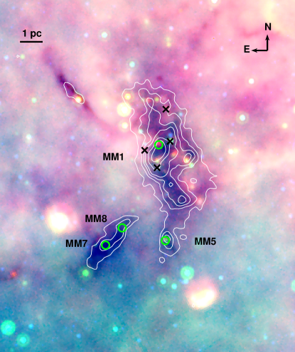
Figure 1.— Spitzer and Herschel composite image overlaid with 1.2 mm continuum emission of G28.53 taken from Rathborne et al. (2006). The colors represent emission at 8.0 µm (blue), 24 µm (green), and 70 µm (red) (Churchwell et al., 2009; Carey et al., 2009; Molinari et al., 2010). The contours levels are 30 (3$\sigma$), 60, 90, 120, 180, 240 mJy per beam. The four clumps, MM1, MM5, MM7, and MM8 are marked. The green circles mark MM1-p1, MM5-1, MM7-p1, and MM8-p1, the most massive cores in each clump. The four crosses mark the H₂O masers.

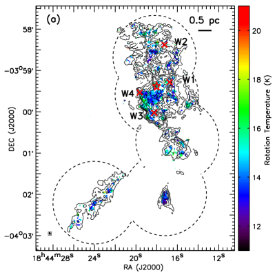
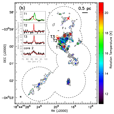
Figure 2.— NH₃ rotation temperature of G28.53. (a) Temperature map using the combined GBT and VLA data, overlaid with contours of the integrated intensities of the NH₃ (1,1) main hyperfine line. The contours are in steps of 5 mJy beam^-1 km s^-1$\times$[3, 6, 9, 12, 15, 20, 25]. The dash circles represent the 2′ primary beams of the VLA observations. ‘Core 2’ in MM1 is marked with a star. The four H₂O masers are marked with crosses and labelled as W1–W4. (b) Temperature map using the VLA data only, overlaid with contours of the integrated intensities of the NH₃ (1,1) main hyperfine line. The contours are in steps of 5 mJy beam^-1 km s^-1$\times$[3, 6, 9, 12, 15, 20]. The three positions exhibiting NH₃ (3,3) emission are marked with circles and labelled as T1–T3, with their spectra and the best gaussian fitting shown in the inset. Note that the two maps are plotted using the same color scale from 11 K to 21 K to show their similarity, but the highest temperature in (a) is 19 K.

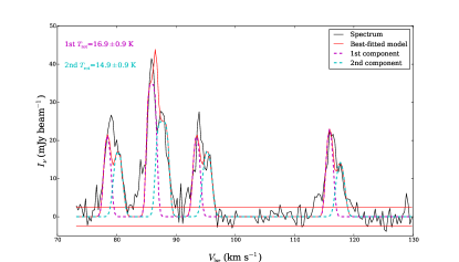
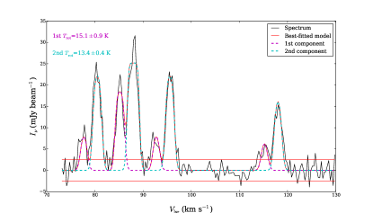
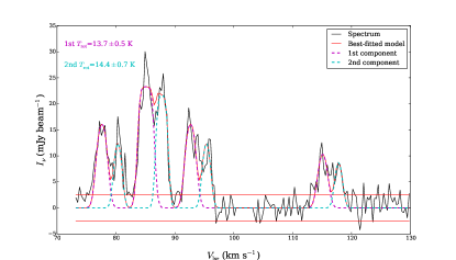
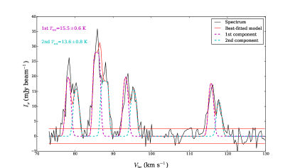
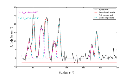
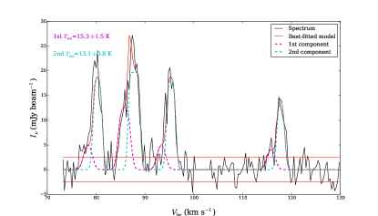
Figure 3.— Two-components fitting of mean spectra of the cores in MM1. The results are listed in Table 3. The NH₃ (1,1) spectra are between 70 and 100 km s^-1, while the NH₃ (2,2) spectra are shifted by 30 km s^-1 to be between $\sim$105 and 130 km s^-1, so that they can be fitted simultaneously. For each spectrum, the dashed magenta and cyan curves represent the two components that are fitted, while the solid red curve represent the sum of them. The horizontal solid lines mark the 3$\sigma$ levels of each spectrum.

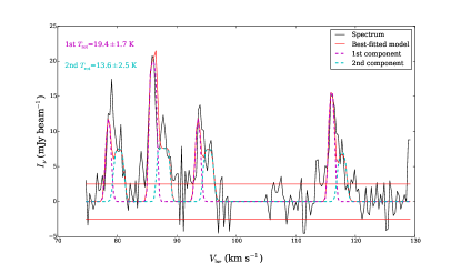
Figure 4.— Two-components fitting of mean spectra of MM1-p1, using the VLA data only. The legends are the same as in Figure 3.

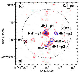
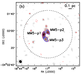
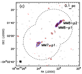
Figure 5.— The SMA 1.3 mm continuum emission of MM1, MM5 and MM7/8. The dashed circles in each panel mark the 56″ primary beams of the SMA. The ellipses mark FWHM of the 2D gaussians fitted to each core. (a) The contours are in steps of 1.1 mJy beam^-1$\times$[$-$5, $-3$, 3, 5, 7, 9, 15, 25, 35, 45]. The two H₂O masers, W1 and W4, are marked with crosses. (b) The contours are in steps of 0.9 mJy beam^-1$\times$[$-3$, 3, 5, 7]. (c) The contours are in steps of 0.81 mJy beam^-1$\times$[$-3$, 3, 5, 7].

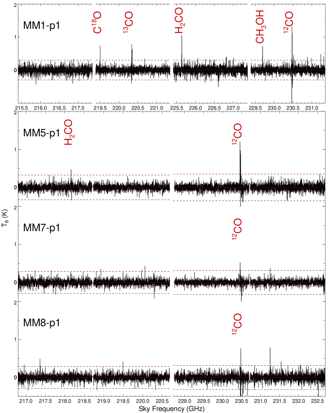
Figure 6.— Spectral lines of MM1-p1, MM5-p1, MM7-p1, and MM8-p1 detected by the SMA. The detected species are labelled in each panel. The horizontal dashed lines mark the 3$\sigma$ levels of each spectrum.

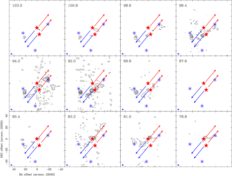
Figure 7.— SMA CO channel maps of MM1. The contours are in steps of 0.1 Jy beam^-1$\times$[-5,5,10,15,20,25,30]. MM1-p1 and MM1-p2 are marked with two stars. The two CO outflows are represented by arrows, with colors indicating blue or red shifted components. The three H₂O masers, W1, W3, and W4 are marked with asterisks.

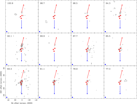
Figure 8.— SMA CO channel maps of MM5. The contours are in steps of 0.05 Jy beam^-1$\times$[-5,5,10,15]. The three cores in MM5 are marked with stars. The arrows represent the CO outflow with colors indicating blue or red shifted component.

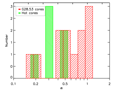
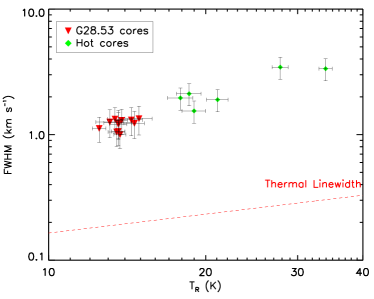
Figure 9.— Left: Virial parameters of cores in G28.53 as well as in the hot core sample of Lu et al. (2014). Constant radial density profiles are assumed for all cores. Right: FWHM linewidths vs. rotation temperatures of cores in G28.53 as well as in the hot core sample of Lu et al. (2014).

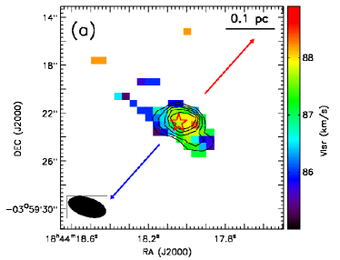
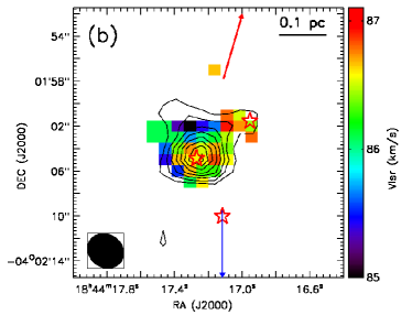
Figure 10.— (a) SMA CH₃OH velocity field of MM1-p1, overlaid with its integrated intensity. The contours are in steps of 0.13 Jy beam^-1 km s^-1$\times$[3, 5, 7, 9, 11]. The star marks MM1-p1. The red and blue arrows represent the CO outflow associated with MM1-p1 as in Figure 7. (b) SMA H₂CO velocity field of MM5, overlaid with its integrated intensity. The contours are in steps of 0.1 Jy beam^-1 km s^-1$\times$[3, 5, 7, 9, 11, 13, 15, 17]. The three stars mark MM5-p1–p3. The red and blue arrows represent the CO outflow in MM5 as in Figure 8.

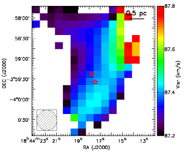
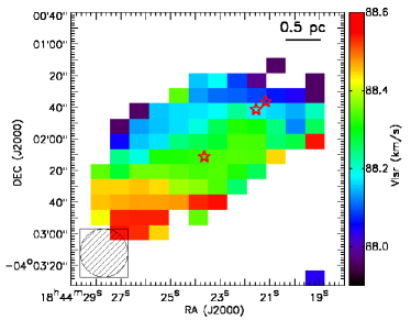
Figure 11.— GBT NH₃ (2,2) velocity field of MM1 (the 87 km s^-1 component) and MM7/8. The 30″ beam of GBT at K band is shown in the lower left corner in each panel. Left: MM1-p1/p2 are marked with stars. Right: MM7-p1 and MM8-p1/p2 are marked with stars.

References

- Beuther et al. (2005) Beuther, H., Schilke, P., Menten, K. M., et al. 2005, ApJ, 633, 535
- Beuther et al. (2002) Beuther, H., Schilke, P., Sridharan, T. K., et al. 2002, A&A, 383, 892
- Beuther et al. (2013) Beuther, H., Linz, H., Tackenberg, J., et al. 2013, A&A, 553, A115
- Blake et al. (1987) Blake, G. A., Sutton, E. C., Masson, C. R., & Phillips, T. G. 1987, ApJ, 315, 621
- Burkert & Bodenheimer (2000) Burkert, A. & Bodenheimer, P. 2000, ApJ, 543, 822
- Carey et al. (2009) Carey, S. J., Noriega-Crespo, A., Mizuno, D. R., et al. 2009, PASP, 121, 76
- Churchwell et al. (2009) Churchwell, E., Babler, B. L., Meade, M. R., et al. 2009, PASP, 121, 213
- Cortes & Crutcher (2006) Cortes, P., & Crutcher, R. M. 2006, ApJ, 639, 965
- Elitzur et al. (1989) Elitzur, M., Hollenbach, D. J., & McKee, C. F. 1989, ApJ, 346, 983
- Fallscheer et al. (2009) Fallscheer, C., Beuther, H., Zhang, Q., Keto, E., & Sridharan, T. K. 2009, A&A, 504, 127
- Frau et al. (2014) Frau, P., Girart, J. M., Zhang, Q., & Rao, R. 2014, A&A, 567, A116
- Furuya et al. (2001) Furuya, R. S., Kitamura, Y., Wootten, H. A., Claussen, M. J., & Kawabe, R. 2001, ApJ, 559, L143
- Girart et al. (2013) Girart, J. M., Frau, P., Zhang, Q., et al. 2013, ApJ, 772, 69
- Goldsmith (2001) Goldsmith, P. F. 2001, ApJ, 557, 736
- Güver & Özel (2009) Güver, T., & Özel, F. 2009, MNRAS, 400, 2050
- Guzmán et al. (2011) Guzmán, V., Pety, J., Goicoechea, J. R., Gerin, M., & Roueff, E. 2011, A&A, 534, A49
- Henshaw et al. (2013) Henshaw, J. D., Caselli, P., Fontani, F., et al. 2013, MNRAS, 428, 3425
- Ho et al. (2004) Ho, P. T. P., Moran, J. M., & Lo, K. Y. 2004, ApJ, 616, L1
- Ho & Townes (1983) Ho, P. T. P., & Townes, C. H. 1983, ARA&A, 21, 239
- Li et al. (2003) Li, D., Goldsmith, P. F., & Menten, K. 2003, ApJ, 587, 262
- Liu et al. (2012) Liu, H. B., Jiménez-Serra, I., Ho, P. T. P., et al. 2012, ApJ, 756, 10
- Lu et al. (2014) Lu, X., Zhang, Q., Liu, H. B., Wang, J., & Gu, Q. 2014, ApJ, 790, 84
- MacLaren et al. (1988) MacLaren, I., Richardson, K. M., & Wolfendale, A. W. 1988, ApJ, 333, 821
- Mangum et al. (1992) Mangum, J. G., Wootten, A., & Mundy, L. G. 1992, ApJ, 388, 467
- McMullin et al. (2007) McMullin, J. P., Waters, B., Schiebel, D., Young, W., & Golap, K. 2007, in Astronomical Society of the Pacific Conference Series, Vol. 376, Astronomical Data Analysis Software and Systems XVI, ed. R. A. Shaw, F. Hill, & D. J. Bell, 127
- Molinari et al. (2010) Molinari, S., Swinyard, B., Bally, J., et al. 2010, A&A, 518, L100
- Peretto et al. (2013) Peretto, N., Fuller, G. A., Duarte-Cabral, A., et al. 2013, A&A, 555, A112
- Pillai et al. (2011) Pillai, T., Kauffmann, J., Wyrowski, F., et al. 2011, A&A, 530, A118
- Pillai et al. (2006) Pillai, T., Wyrowski, F., Carey, S. J., & Menten, K. M. 2006, A&A, 450, 569
- Qiu et al. (2013) Qiu, K., Zhang, Q., Menten, K. M., Liu, H. B., & Tang, Y.-W. 2013, ApJ, 779, 182
- Qiu et al. (2014) Qiu, K., Zhang, Q., Menten, K. M., et al. 2014, ApJ, 794, L18
- Rathborne et al. (2010) Rathborne, J. M., Jackson, J. M., Chambers, E. T., et al. 2010, ApJ, 715, 310
- Rathborne et al. (2006) Rathborne, J. M., Jackson, J. M., & Simon, R. 2006, ApJ, 641, 389
- Rathborne et al. (2008) Rathborne, J. M., Jackson, J. M., Zhang, Q., & Simon, R. 2008, ApJ, 689, 1141
- Reid et al. (2009) Reid, M. J., Menten, K. M., Zheng, X. W., et al. 2009, ApJ, 700, 137
- Sanhueza et al. (2012) Sanhueza, P., Jackson, J. M., Foster, J. B., et al. 2012, ApJ, 756, 60
- Sault et al. (1995) Sault, R. J., Teuben, P. J., & Wright, M. C. H. 1995, in Astronomical Society of the Pacific Conference Series, Vol. 77, Astronomical Data Analysis Software and Systems IV, ed. R. A. Shaw, H. E. Payne, & J. J. E. Hayes, 433
- Schneider et al. (2014) Schneider, N., Csengeri, T., Klessen, R. S., et al. 2014, arXiv:1406.3134
- Simon et al. (2006) Simon, R., Rathborne, J. M., Shah, R. Y., Jackson, J. M., & Chambers, E. T. 2006, ApJ, 653, 1325
- Strittmatter (1966) Strittmatter, P. A. 1966, MNRAS, 132, 359
- Swade (1989) Swade, D. A. 1989, ApJ, 345, 828
- Swift (2009) Swift, J. J. 2009, ApJ, 705, 1456
- Szymczak et al. (2005) Szymczak, M., Pillai, T., & Menten, K. M. 2005, A&A, 434, 613
- Walmsley & Ungerechts (1983) Walmsley, C. M., & Ungerechts, H. 1983, A&A, 122, 164
- Wang et al. (2012) Wang, K., Zhang, Q., Wu, Y., Li, H.-b., & Zhang, H. 2012, ApJ, 745, L30
- Wang et al. (2011) Wang, K., Zhang, Q., Wu, Y., & Zhang, H. 2011, ApJ, 735, 64
- Wang et al. (2014) Wang, K., Zhang, Q., Testi, L., et al. 2014, MNRAS, 439, 3275
- Wang et al. (2006) Wang, Y., Zhang, Q., Rathborne, J. M., Jackson, J., & Wu, Y. 2006, ApJ, 651, L125
- Wu et al. (2009) Wu, P.-F., Takakuwa, S., & Lim, J. 2009, ApJ, 698, 184
- Zhang et al. (2005) Zhang, Q., Hunter, T. R., Brand, J., et al. 2005, ApJ, 625, 864
- Zhang et al. (2001) —. 2001, ApJ, 552, L167
- Zhang & Wang (2011) Zhang, Q., & Wang, K. 2011, ApJ, 733, 26
- Zhang et al. (2009) Zhang, Q., Wang, Y., Pillai, T., & Rathborne, J. 2009, ApJ, 696, 268
- Zhang et al. (2014) Zhang, Q., Qiu, K., Girart, J. M., et al. 2014, ApJ, 792, 116