From Causal Dynamical Triangulations
To Astronomical Observations

Abstract

This letter discusses phenomenological aspects of dimensional reduction predicted by the Causal Dynamical Triangulations (CDT) approach to quantum gravity. The deformed form of the dispersion relation for the fields defined on the CDT space-time is reconstructed. Using the Fermi satellite observations of the GRB 090510 source we find that the energy scale of the dimensional reduction is $E_{*}>0.7\sqrt{4-d_{\rm UV}}\cdot 10^{10}$ GeV at (95 $\%$ CL), where $d_{\rm UV}$ is the value of the spectral dimension in the UV limit. By applying the deformed dispersion relation to the cosmological perturbations it is shown that, for a scenario when the primordial perturbations are formed in the UV region, the scalar power spectrum $\mathcal{P}_{S}\propto k^{n_{S}-1}$ where $n_{S}-1\approx\frac{3r(d_{\rm UV}-2)}{(d_{\rm UV}-1)r-48}$. Here, $r$ is the tensor-to-scalar ratio. We find that within the considered model, the predicted from CDT deviation from the scale-invariance ($n_{S}=1$) is in contradiction with the up to date Planck and BICEP2.

1 Introduction

The littleness of the Planck length is indescribable. The immense size the observable Universe is paralyzing. However, the geometric mean of the two characteristic values results in a tangible quantity. Explicitly, $\sqrt{1l_{\rm Pl}\cdot 1{\rm Gpc}}\approx 1{\rm mm}$, where the Planck length $l_{\rm Pl}\approx 1.62\cdot 10^{-35}$ m and the gigaparsec $1{\rm Gpc}\approx 3.09\cdot 10^{28}$ m.

As we will see from the analysis performed in the letter, better understanding of both the super-short and super-large scales can be gained thanks to this property.

So, how does it work? There are two main possibilities. The first one is a result of accumulation of the tiny Planck scale deviations acting on particles propagating across cosmological distances. The second possibility exploits the evolution of the Universe. The Universe is as big as it is because it is expanding. As a result, the Planck scale in the early universe, multiplied by the growth factor becomes macroscopic in the mature universe. In both cases, the multiplication law brings the Planck scale closer to the scales of our perception.

We do not know yet what the Planck scale physics is. However, by taking the use of the compensation of scales discussed above, one may already try to falsify the theoretical models of quantum gravitational phenomena, which we have.

The theory of Planck scale physics which we are going to examine here are Causal Dynamical Triangulations (CDT) [1, 2]. The theory is a non-perturbative approach based on the path integral formulation of quantum mechanics. The crucial ingredient of the theory is a causality condition imposed at the level of Wick-rotated time coordinate. In similarity to statistical physics, the different space-time configurations are evaluated using Monte Carlo computer simulations.

Various promising results arose from numerical studies of the quantum gravitational system with the positive cosmological constant. One of the most profound is the emergence of four dimensional de Sitter space-time [3, 4] in the so-called phase C. However, as reflected by features of the process of diffusion taking place at the simplicial manifold of CDT, the reconstructed de Sitter space-time is not fully classical.

In particular, it has been shown that the spectral dimension characterizing the diffusion process can be parametrized in the following way [6]:

$$d_{S}(\sigma)=a-\frac{b}{c+\sigma},$$ (1)

where $\sigma$ is the diffusion time. At the representative point in phase C ($\kappa_{0}=2.2$, $\Delta=0.6$) the values $a=4.02$, $b=119$ and $c=54$ [6] and $a=4.06$, $b=135$ and $c=67$ [7] have been obtained from numerical simulations. In both cases, four dimensional space-time ($d_{S}\approx 4$) is correctly recovered in the IR limit ($\sigma\rightarrow\infty$). However, in the UV limit ($\sigma\rightarrow 0$) dimensional reduction to $d_{S}\approx 2$ was observed. This effect is not reserved to CDT only and has been noticed in other approaches to quantum gravity as well [8]. Moreover, recent numerical studies revealed that the UV behavior of the spectral dimension may change depending on which part of the phase C is considered. In particular, in has been shown that when $C-A$ transition line is approached, the UV limit of the spectral dimension is consistent with $d_{S}\approx 3/2$ [7]. Worth noticing is that, such value of the spectral dimension may have theoretical relevance (see Ref. [9]). In what follows, we will refer to two different UV values of the spectral dimension mentioned above. However, the performed calculations will allow to consider also other possible values of the spectral dimension in the UV limit.

The expression (1) is a starting point for our further considerations. After fixing the IR value $d_{S}$ to be precisely equal to the topological space-time dimension $d=4$ and we obtain

$$d_{S}(\sigma)=4-\frac{4-d_{\rm UV}}{1+\sigma/c},$$ (2)

such that $d_{\rm UV}:=d_{S}(\sigma\rightarrow 0)$ is the value of the spectral dimension in the UV limt. The parameter $c$ can be related to the energy scale of the dimensional reduction: $E_{*}:=\frac{1}{\sqrt{c}}$. The diffusion time $\sigma$ introduces an external parametrization of the diffusion process on a given space-time. Worth mentioning here is that, due to absorption of diffusion constant in the heat kernel equation, the dimensionality of $\sigma$ is (in the Planck units) an inverse energy squared.

2 From the spectral dimension to the deformed dispersion relation

The spectral dimension discussed in the previous section is formally defined as follows

$$d_{S}(\sigma)\equiv-2\frac{\partial\log P(\sigma)}{\partial\log\sigma},$$ (3)

where

$$P(\sigma)=\int d\mu e^{\sigma\triangle_{p}}$$ (4)

is the average return probability of the random walk (diffusion) process. Here, $d\mu$ is the invariant measure in the momentum space, which we assume to be the classical one $d\mu=\frac{dEd^{3}{\vec{p}}}{(2\pi)^{4}}$. $\triangle_{p}$ is the Laplace operator in momentum space. In the case of the Euclidean 4-dimensional space $\triangle_{p}=-E^{2}-\vec{p}^{2}$. This expression might be viewed as the Wick rotated $(E\rightarrow iE)$ version of the analogous formula in the Minkowski space $\triangle_{p}=E^{2}-\vec{p}^{2}$, which defines dispersion relation for the free fields living on the space-time ($\triangle_{p}=0\Rightarrow E^{2}=\vec{p}^{2}$). In this case, the equations (3) and (4) predict $d_{S}=d$, where $d=4$ is the topological dimension.

CDT predicts that the spectral dimension varies as a function of the diffusion time $\sigma$. The corresponding momentum Laplace operator has to be, therefore, deformed with respect to the classical case. Here, we parametrize this departure in the following manner

$$\triangle_{p}=-E^{2}-\Omega(p)^{2},$$ (5)

where $\Omega(p)$ is some unknown function of $p:=\sqrt{\vec{p}\cdot\vec{p}}$.

The parametrization (5) is of course one of many possible ones. In general, both the energy and momentum parts could be deformed, including also mixed terms. Recovering the form of the deformed momentum Laplace operator based on a single function $d_{S}(\sigma)$ is, therefore, a highly ambiguous problem in general. This is because different forms of the deformed momentum Laplace operator may lead to the same (or very similar) shape of the diffusion-time dependence of the spectral dimension (For more detailed discussion of the ambiguity issue we refer to Ref. [11]). The choice (5) has been made such that there is only a single unknown function involved, which form can unambiguously recovered. The fact that in the applied parametrization the energy part is not a subject of modification is supported by the CDT results. Namely, in CDT the time direction is imposed by time foliation and contribute classically. The same is, therefore, expected for energy. On the other hand, spatial slices have fractal structure, leading to the dimensional reduction (see Ref. [12]). In consequence, corrections to the momentum part of the Laplace operator are expected. Furthermore, the choice (5) is the most conservative one and has simple physical interpretation because it leads to the dispersion relation in the form $E=\Omega(p)$.

The task would be now to recover the form of the function $\Omega(p)$ for the CDT spectral dimension (2). In this case, the expression for the return probability is

$$P(\sigma)=\frac{1}{\sqrt{4\pi\sigma}}\frac{4\pi}{(2\pi)^{2}}\int_{0}^{\infty}dp\ p^{2}e^{-\sigma\Omega^{2}(p)},$$ (6)

where integrations over $E$ and the angular part of $d^{3}\vec{p}\$ have been performed. As it has been shown in Ref. [13], the relation (6) can be converted into the form of the inverse Laplace transform

$$p^{3}=\frac{1}{2\pi i}\lim_{T\rightarrow\infty}\int^{\gamma+iT}_{\gamma-iT}\left(12\pi^{5/2}\frac{P(\sigma)}{\sqrt{\sigma}}\right)e^{\sigma\Omega^{2}(p)}d\sigma,$$ (7)

the $\gamma\in\mathbb{R}$ has to satisfy the condition $\forall_{\sigma_{*}}\gamma>\Re(\sigma_{*})$, where $\sigma_{*}$ denotes singularities of $P(\sigma)/\sqrt{\sigma}$. The $P(\sigma)$ function is recovered by integrating definition (3) with use of parametrization (2). We find that

$$P(\sigma)=\frac{1}{16\pi^{2}\sigma^{d_{\rm UV}/2}(\sigma+c)^{2-d_{\rm UV}/2}},$$ (8)

which is a positive definite function and, therefore, has correct probabilistic interpretation. By applying (8) to (7) the following deformed dispersion relation is obtained:

$$p^{3}=\Omega^{3}{{}_{1}F_{1}}\left(2-d_{\rm UV}/2,5/2;-c\Omega^{2}\right),$$ (9)

where ${{}_{1}F_{1}}(a,b;z)$ is the confluent hypergeometric function. Equation (9), is an entangled form of the deformed dispersion relation $E=\Omega(p)$. The function $\Omega(p)$ for $d_{\rm UV}=2$ and $d_{\rm UV}=3/2$ is shown in Fig. 1.

Figure 1: A plot of exemplary dispersion relations predicted by dimensional reduction in Causal Dynamical Triangulations. The continuous line represents the $d_{\rm UV}=2$ case while the dashed line corresponds to $d_{\rm UV}=3/2$.

In the IR limit $(p\rightarrow 0)$ the dispersion relation is approximated by

$$\Omega_{\rm IR}(p)\approx p+\frac{E_{*}}{15}(4-d_{\rm UV})\left(\frac{p}{E_{*}}\right)^{3},$$ (10)

so the classical limit is correctly recovered. However, when passing to the high energy range (the UV limit) the dispersion relation undergoes deflection to the form

$$\Omega_{\rm UV}(p)\approx E_{*}b\left(\frac{p}{E_{*}}\right)^{\frac{3}{d_{\rm UV}-1}}\propto p^{\frac{3}{d_{\rm UV}-1}},$$ (11)

where for the further convince we introduce

$$b:=\left(\frac{4\Gamma(d_{\rm UV}/2+1/2)}{3\sqrt{\pi}}\right)^{\frac{1}{d_{\rm UV}-1}},$$ (12)

which is defined such that $b(d_{\rm UV}=4)=1$ and $b(d_{\rm UV}=2)=\frac{2}{3}$ and $b(d_{\rm UV}=3/2)\approx 0.465$. For $d_{\rm UV}=2$ we have $\Omega_{\rm UV}(p)\propto p^{3}$ and for $d_{\rm UV}=3/2$ the $\Omega_{\rm UV}(p)\propto p^{6}$.

Both of the obtained limiting behaviors of the deformed dispersion relation will now be used to construct the relation of CDT to astrophysical and cosmological observations.

3 Astrophysics

The dispersion relation derived in the previous section can now be used to find the group velocity of photons. For the particles having energy $E\ll E_{*}$ the IR limit approximation (10) may be applied, leading to the quadratic deviation

$$v_{\rm gr}:=\frac{\partial E}{\partial p}=\frac{\partial\Omega(p)}{\partial p}\approx 1+\frac{3}{15}(4-d_{\rm UV})\left(\frac{E}{E_{*}}\right)^{2}.$$ (13)

This expression predicts that the group velocity is increasing (superluminal behavior) or decreasing (subluminal behavior) with the energy depending on whether $d_{\rm UV}$ is smaller or greater than four respectively. In case of the dimensional reduction expected in the phase C of CDT, for a bunch of photons of different energies emitted simultaneously the ones with the highest energy will arrive first to the observer. This effect can be quantified by the arrival time difference between $E$ and $E\rightarrow 0$ energy photons. With use of formula (13), the corresponding expression is $\tau\simeq-L\frac{3}{15}(4-d_{\rm UV})\left(\frac{E}{E_{*}}\right)^{2}$, where $L$ is the distance to a source. Although a huge value of the energy scale $E_{*}$ is expected, the multiplication by a sufficiently large distance $L$ may bring the value of $\tau$ close to the observational window.

The effect can be constrained with use of the signals from the high-energy astrophysical sources such as gamma ray bursts (GRB) [14]. In particular, the GRB 090510 remote by $L\approx 5,8$ Mpc may be used. Using the data from the Fermi-Large Area Telescope [16] one can find that constraints on the energy scale of the dimensional reduction are:

$$E_{*}>0.7\sqrt{4-d_{\rm UV}}\cdot 10^{10}\text{GeV at}\ (95\%\text{CL})\ \text{for}\ d_{\rm UV}<4,$$

$$E_{*}>4.8\sqrt{d_{\rm UV}-4}\cdot 10^{10}\text{GeV at}\ (95\%\text{CL})\ \text{for}\ d_{\rm UV}>4.$$

These constraints are definitely much stronger than any obtained from the accelerator physics experiments (which are reaching energies of the order of $10^{4}$ GeV). However, because of the quadratic (in energy) from of the effect, the constraint is distant from the Planck scale Furthermore, the obtained values of constrains are typical to the quadratic corrections, which are obtained in various approaches to quantum gravity (see Ref. [15] for recent review).

On the other hand, in case when one would consider the high energy photons to be described by the UV part of the dispersion relation, the group velocity is given by

$$v_{\rm gr}^{\rm UV}=\frac{\partial\Omega_{\rm UV}(p)}{\partial p}=\frac{3b}{d_{\rm UV}-1}\left(\frac{E}{bE_{*}}\right)^{\frac{4-d_{\rm UV}}{3}}.$$ (14)

Such a situation is, however, very unlikely because it would require photons with energies $E>E_{*}$ to be considered and as shown previously this corresponds to energies above $10^{10}$ GeV.

4 Cosmology

Because of the quadratic nature of the IR variation of the group velocity, perhaps the more promising is an application of dimensional reduction to cosmology. Here, instead of the IR, the UV part of the dispersion relation will play a crucial role. The potential relevance of the UV scaling of the modified dispersion relation in cosmology has been suggested in Ref. [17]. It has been shown that dimensional reduction to $d_{\rm UV}=2$ leads to the scale invariant vacuum fluctuations of the primordial perturbations in the UV domain. What has not been shown is how the shape of the spectrum changes when we try to relate it with the one that is observationally relevant. Here, we show that a deviation from $d_{\rm UV}=2$ leads to a tilt in the power spectrum. This prediction is confronted with the observations of the cosmic microwave background radiation (CMB).

The resulting CDT dispersion relation $E=\Omega(p)$ can be incorporated into the equation of modes for the cosmological perturbations. For this purpose let us consider equation of modes

$$\frac{d^{2}}{d\tau^{2}}f_{k}+\left(-\nabla^{2}_{k}-\frac{z^{{}^{\prime\prime}}}{z}\right)f_{k}=0,$$ (15)

where $\nabla^{2}_{k}$ is the momentum part of the total Laplace operator, which in the classical $3+1$ case is equal $\nabla^{2}_{k}=-k^{2}$. Having a given value of $k$ the corresponding physical value of momentum can be find from the expression $p=\frac{k}{a}$, where $a$ is the scale factor. The value of $z$ depends on which kind of perturbations is considered. For the gravitational waves $z=z_{T}:=a$ and for the scalar perturbations $z=z_{S}:=a\frac{\dot{\phi}}{H}$.

The task now is to phenomenologically introduce the CDT effects to Eq. 15 by modifying the the expression for $\nabla^{2}_{k}$. This can be done by using the dispersion momentum part of the Laplace operator (5). However, this require a proper rescaling which will take into account relation between the physical momentum $p$ present in the $\Omega(p)$ function and the coordinate momentum $k$ appearing while the cosmological case is considered. By performing the following replacement

$$-\nabla^{2}_{k}\rightarrow a^{2}\Omega^{2}(k/a),$$ (16)

in Eq. 15, the effect of deformed dispersion relation can be introduced, such that the classical limit classical limit $a^{2}\Omega^{2}(k/a)\rightarrow a^{2}(k/a)^{2}=k^{2}$ is recovered correctly for $p\rightarrow 0$. Worth stressing here is that in the above analysis we assumed that the averaged background dynamics is not a subject of the CDT corrections. This is satisfied in the regime where the homogeneous dynamics is well approximated by the classical cosmology but the inhomogeneities, if considered at sufficiently small spatial scales, reflect quantum nature of the underlying spacetime.

In consequence, in the sub-Hubble limit $\left(a^{2}\Omega^{2}(k/a)\gg\frac{z^{{}^{\prime\prime}}}{z}\right)$, the (Bunch-Davies) vacuum normalization of the $f_{k}$ mode functions leads to

$$|f_{k}|^{2}=\frac{1}{2a\Omega(k/a)}.$$ (17)

Applying this to the definition of the scalar power spectrum we find that for $k/a\gg E_{*}$

$$\mathcal{P}_{S}(k) :=\frac{k^{3}}{2\pi^{2}}\frac{|f_{k}|^{2}}{z_{S}^{2}}$$ (18)

$$=\frac{\left(\frac{E_{*}}{E_{\rm Pl}}\right)^{2}\left(\frac{1}{E_{*}}\frac{k}{a}\right)^{\frac{3(d_{\rm UV}-2)}{d_{\rm UV}-1}}}{3\pi(1+w)b}\propto k^{n_{S}-1},$$

where $n_{S}=1+\frac{3(d_{\rm UV}-2)}{d_{\rm UV}-1}$. Furthermore, we assume that the universe is filled with barotropic matter: $P=w\rho$, with $w=const$.

Indeed, for $d_{\rm UV}=2$ the power spectrum (18) becomes scale invariant $\mathcal{P}_{S}(k)=\frac{1}{\pi(1+w)}\left(\frac{E_{*}}{E_{\rm Pl}}\right)^{2}=const$. While it is tempting to relate the obtained spectrum with that inferred from the CMB nearly scale-invariant spectrum of the primordial perturbations, it is not allowed to do so directly. The spectrum (18) corresponds to the UV regime ($k/a\gg E_{*}$) which has to be suitably converted into the super-Hubble spectrum probed observationally. In general, this would require evolving the modes starting from the UV domain until crossing the Hubble horizon. This will unavoidably affect the shape of the power spectrum. A scenario in which knowledge of the intermediate evolution is not required corresponds to the case when the Hubble horizon is located in the UV domain (in the sense of the deformed dispersion relation). In that case freezing of the modes occurs already at the level of the UV spectrum (18). The freeze out considered here is the same as the one consider in the classical cosmology and is related with the fact that in the super-Hubble limit the Eq. 15 reduces to $\frac{d^{2}}{d\tau^{2}}f_{k}-\frac{z^{{}^{\prime\prime}}}{z}f_{k}\approx 0$, such that physical amplitude of perturbation i.e. $\frac{f_{k}}{z}$ has solution in the form $\frac{f_{k}}{z}=A_{k}+B_{k}\int\frac{d\tau}{z^{2}}$, where the effect of freeze out is because of non-vanishing constant of integration $A_{k}$.

In scenario under consideration the tensor-to-scalar ratio can be expressed as

$$r :=\frac{\mathcal{P}_{T}(k_{0})}{\mathcal{P}_{S}(k_{0})}=\frac{64\pi G\frac{k^{3}}{2\pi^{2}}\frac{|f_{k}|^{2}}{z_{T}^{2}}}{\frac{k^{3}}{2\pi^{2}}\frac{|f_{k}|^{2}}{z_{S}^{2}}}$$ (19)

$$=64\pi G\left(\frac{z_{S}}{z_{T}}\right)^{2}=24(1+w),$$

can be directly related to the CMB data. The best current observational bound at the pivot scale $k_{0}=0.05\ {\rm Mpc}^{-1}$ is $r<0.07$ at 95 % confidence level (BICEP2/Keck Array) [18], which implicates that $w<-0.997$ when the perturbations were formed. The universe had to, therefore, be very close to the de Sitter phase when the perturbations were formed. Cosmic inflation is still needed!

The value of the power spectrum accessible observationally is at the horizon-crossing. In our case, the horizon-crossing condition $a^{2}\Omega^{2}(k/a)=\frac{z^{{}^{\prime\prime}}}{z}$ translates into $k\simeq aE_{*}\left(\frac{H}{E_{*}b}\right)^{\frac{d_{\rm UV}-1}{3}}$ $:=k_{H}$ for $H>E_{*}$. Using this, the spectral index of scalar perturbations at the horizon-crossing is

$$n_{S}-1\equiv\frac{d\ln\mathcal{P}_{S}(k=k_{H})}{d\ln k}\approx\frac{3r(d_{\rm UV}-2)}{(d_{\rm UV}-1)r-48}.$$ (20)

The scale invariance is still recovered for $d_{\rm UV}=2$. However, according to the most up to date observations, the scalar power spectrum exhibits a red tilt. In particular, the Planck satellite measurements provide following value of the spectral index: $n_{S}=0.9616\pm 0.0094$ [19]. In Fig. 2 we compare predictions of the formula (20) with the Planck data for representative values of the tensor-to-scalar ratio $r$.

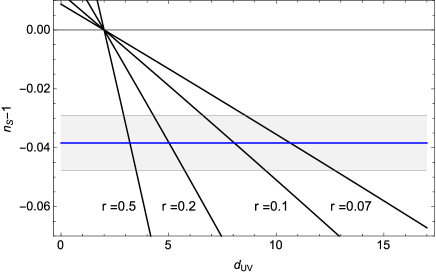
Figure 2: The black lines represent function (20) plotted for fixed values of $r$. The horizontal blue line corresponds to the value $n_{S}-1=-0.0384$ obtained based on the Planck satellite measurements [19]. The shadowed region represents uncertainty of the measurement.

Analysis of of the Fig. 2 indicates that it is impossible to explain observational data with the values of $d_{\rm UV}$ expected in the phase $C$ of CDT. That would require the value of the $r$ parameter to be greater than the observational bound $r<0.07$. For $d_{\rm UV}=4$ the model reduces to the classical inflation with barotropic equation of state with $w$ being very close to $w=-1$, which is disfavored by the observational data . A consistency with the observational data (both the value of the spectral index and the tensor-to-scalar ratio) can be obtained only by taking

$$d_{\rm UV}>10.65.$$ (21)

However, this value is in overt contradiction with the values of $d_{\rm UV}$ expected in the C phase of CDT. The scenario considered can be, therefore, ruled out based on the CMB data. Other scenarios, such as those with $H<E_{*}$ at the horizon-crossing have to be studied separately, taking into account the evolution of modes in the intermediate energy range. Also, it has to be stressed that the analysis has been performed for the background dynamics described by the barotropic fluid. Extension of the presented results e.g. to the case of slow-roll is deserved.

What we have actually shown is that the dimensional reduction does not provide a mechanism which can be competitive to the inflationary generation of primordial inhomogeneities. An attempt of using the UV-modified Bunch Davies vacuum, in particular corresponding to the promising $d_{\rm UV}=2$ case, did not lead to the nearly scale-invariant spectrum being consistent with cosmological observations. However, there is also a positive outcome of the performed analysis. The presented calculations indicate that the large values of $d_{\rm UV}$, satisfying the condition (21), lead the results being consistent with observations. Moreover, such super-diffusion type of behavior may improve fitting properties of the classical models which were not favored by the cosmological observations, as observed in the analyzed model with barotropic fluid.

Interestingly, the increase of the spectral dimension above $d_{S}=4$ has been observed in CDT in both, the $B$-phase and the so-called bifurcation sub-phase of the C-phase. Further detailed analysis has to be performed to verify if the presented analysis can be applied to any of these cases. Furthermore, while the super-diffusion type of behavior is not typically predicted within the models of Planck scale physics, it has been observed in Relative Locallity [21] and in the models inspired by the Bekenstein-Hawking entropy-area scaling [22].

5 Conclusions

The results presented in this letter neither prove nor disprove Causal Dynamical Triangulations. What has been essentially shown is that phenomenology of CDT can be extracted from numerical studies of the spectral dimension. The predicted energy-dependence of the speed of light allowed us to rule out a possibility of low-energy dimensional reduction. Furthermore, by incorporating the predictions regarding the UV behavior of the spectral dimension to primordial cosmology, we found that the CDT-motivated cosmological scenarios may be observationally falsifiable. Moreover, we explicitly ruled out one of them with use of the observations of the CMB.

As Thomas A. Edison once said ‘I have not failed. I’ve just found 10000 ways that won’t work.’ Quoting the sentence, we are convinced that unabated stubbornness in eliminating Planck scale scenarios will eventually lead to a discovery comparable only with Edison’s one.

References

- [1] J. Ambjorn, J. Jurkiewicz and R. Loll, Phys. Rev. Lett. 85 (2000) 924.
- [2] J. Ambjorn, A. Goerlich, J. Jurkiewicz and R. Loll, Phys. Rept. 519 (2012) 127.
- [3] J. Ambjorn, J. Jurkiewicz and R. Loll, Phys. Rev. Lett. 93 (2004) 131301.
- [4] J. Ambjorn, A. Görlich, J. Jurkiewicz and R. Loll, Phys. Rev. Lett. 100 (2008) 091304.
- [5] J. Ambjorn, S. Jordan, J. Jurkiewicz and R. Loll, Phys. Rev. D 85 (2012) 124044.
- [6] J. Ambjorn, J. Jurkiewicz and R. Loll, Phys. Rev. Lett. 95 (2005) 171301.
- [7] D. N. Coumbe and J. Jurkiewicz, JHEP 1503 (2015) 151
- [8] S. Carlip, AIP Conf. Proc. 1196 (2009) 72.
- [9] J. Laiho and D. Coumbe, Phys. Rev. Lett. 107 (2011) 161301
- [10] G. Amelino-Camelia, L. Freidel, J. Kowalski-Glikman and L. Smolin, Phys. Rev. D 84 (2011) 084010.
- [11] G. Calcagni, A. Eichhorn and F. Saueressig, Phys. Rev. D 87 (2013) no.12, 124028
- [12] A. Gorlich, “Causal Dynamical Triangulations in Four Dimensions,” PhD thesis, 2010, arXiv:1111.6938 [hep-th].
- [13] T. P. Sotiriou, M. Visser and S. Weinfurtner, Phys. Rev. D 84 (2011) 104018.
- [14] G. Amelino-Camelia, J. R. Ellis, N. E. Mavromatos, D. V. Nanopoulos, S. Sarkar and , Nature 393 (1998) 763.
- [15] G. Calcagni, JHEP 1703 (2017) 138 Erratum: [JHEP 1706 (2017) 020]
- [16] V. Vasileiou, A. Jacholkowska, F. Piron, J. Bolmont, C. Couturier, J. Granot, F. W. Stecker and J. Cohen-Tanugi et al., Phys. Rev. D 87 (2013) 12, 122001.
- [17] G. Amelino-Camelia, M. Arzano, G. Gubitosi and J. Magueijo, Phys. Rev. D 87 (2013) 12, 123532.
- [18] P. A. R. Ade et al. [BICEP2 and Keck Array Collaborations], Phys. Rev. Lett. 116 (2016) 031302
- [19] P. A. R. Ade et al. [Planck Collaboration], Astron. Astrophys. 571 (2014) A16.
- [20] P. A. R. Ade et al. [Planck Collaboration], Astron. Astrophys. 594 (2016) A20
- [21] M. Arzano and T. Trzesniewski, Phys. Rev. D 89 (2014) no.12, 124024
- [22] M. Arzano and G. Calcagni, Phys. Rev. D 88 (2013) 084017