Robust Recovery of Positive Stream of Pulses

Abstract

The problem of estimating the delays and amplitudes of a positive stream of pulses appears in many applications, such as single-molecule microscopy. This paper suggests estimating the delays and amplitudes using a convex program, which is robust in the presence of noise (or model mismatch). Particularly, the recovery error is proportional to the noise level. We further show that the error grows exponentially with the density of the delays and also depends on the localization properties of the pulse.

I Introduction

Signals comprised of stream of pulses play a key role in many engineering applications, such as ultrasound imaging and radar (see, e.g. [1, 2, 3, 4, 5]). In some applications, the signal under examination is known to be real and non-negative. For instance, in single-molecule microscopy we measure the convolution of positive point sources with the microscope’s point spread function [6, 7, 8]. Another example arises from the problem of estimating the orientations of the white matter fibers in the brain using diffusion weighted magnetic resonance imaging (MRI). In this application, the measured data is modeled as the convolution of a sparse positive signal on the sphere, which represents the unknown orientations, with a known point spread function that acts as a low-pass filter [9, 10].

This paper focuses its attention on the model of positive stream of pulses. In this model, the measurements are comprised of a sum of unknown shifts of a kernel $\mathbf{g}$ with positive coefficients, i.e.

$$\mathbf{y}[k]=\sum_{m}c_{m}\mathbf{g}\left[k-k_{m}\right]+\tilde{\mathbf{n}}[k],\quad k\in\mathbb{Z},\quad c_{m}>0,$$ (I.1)

where $\tilde{\mathbf{n}}$ is a bounded error term (noise, model mismatch) obeying $\left\|{\tilde{\mathbf{n}}}\right\|_{1}:=\sum_{k\in\mathbb{Z}}\left|\tilde{\mathbf{n}}[k]\right|\leq\delta$. We do not assume any prior knowledge on the noise statistics. The pulse $\mathbf{g}$ is assumed to be a sampled version of a scaled continuous kernel, namely, $\mathbf{g}[k]:=\mathbf{g}\left(\frac{k}{\sigma N}\right)$, where $\mathbf{g}(t)$ is the continuous kernel, $\sigma>0$ is a scaling parameter and $1/N$ is the sampling interval. For instance, if $\mathbf{g}$ is Gaussian kernel, then $\sigma$ denotes its standard deviation. The delayed versions of the kernel, $\mathbf{g}\left[k-k_{m}\right]$, are often referred to as atoms. We aim to estimate the set of delays $\left\{k_{m}\right\}\subset\mathbb{Z}$ and the positive amplitudes $\left\{c_{m}>0\right\}$ from the measured data $\mathbf{y}[k]$.

The sought parameters of the stream of pulses model can be defined by a signal of the form

$$\mathbf{x}[k]:=\sum_{m}c_{m}\boldsymbol{\delta}\left[k-k_{m}\right],\quad c_{m}>0,$$ (I.2)

where $\boldsymbol{\delta}[k]$ is the one-dimensional Kronecker Delta function

$$\boldsymbol{\delta}[k]:=\begin{cases}1,&k=0,\\ 0&k\neq 0.\end{cases}$$

In this manner, the problem can be thought of as a sparse deconvolution problem, namely,

$$\mathbf{y}[k]=\left(\mathbf{g}\ast\left(\mathbf{x}+\mathbf{n}\right)\right)[k],$$ (I.3)

where ${}^{\prime}\ast^{\prime}$ denotes a discrete convolution and $\mathbf{n}[k]$ is the error term.

The one-dimensional model can be extended to higher-dimensions. In this paper we also analyze in detail the model of two-dimensional positive stream of pulses given by

$$\mathbf{y}[\mathbf{k}] = \left(\mathbf{g_{2}}\ast\left(\mathbf{x_{2}}+\mathbf{n}\right)\right)\left[\mathbf{k}\right],$$

$$= \sum_{m}c_{m}\mathbf{g_{2}}\left[\mathbf{k}-\mathbf{k}_{m}\right]+\tilde{\mathbf{n}}[\mathbf{k}],$$

where $\mathbf{k}:=\left[k_{1},k_{2}\right]\in\mathbb{Z}^{2}$ and $\mathbf{g_{2}}$ is a two-dimensional pulse. As in the one-dimensional case, the pulse is defined as a sampled version of a two-dimensional kernel $\mathbf{g_{2}}(t_{1},t_{2})$ by $\mathbf{g_{2}}\left[\mathbf{k}\right]=\mathbf{g_{2}}\left(\frac{k_{1}}{\sigma_{1}N_{1}},\frac{k_{2}}{\sigma_{2}N_{2}}\right)$. The signal

$$\mathbf{x}_{2}[\mathbf{k}]:=\sum_{m}c_{m}\boldsymbol{\delta}\left[\mathbf{k}-\mathbf{k}_{m}\right],\quad c_{m}>0,$$ (I.5)

defines the underlying parameters to be estimated, where here $\boldsymbol{\delta}$ denotes the two-dimensional Kronecker Delta function. For the sake of simplicity, we assume throughout the paper that $\sigma_{1}N_{1}=\sigma_{2}N_{2}:=\sigma N$.

Many algorithms have been suggested to recover $\mathbf{x}$ from the stream of pulses $\mathbf{y}$. A naive approach would be to estimate $\mathbf{x}$ via least-squares estimation. However, even if the convolution as in (I.3) is invertible, the condition number of its associated convolution matrix tends to be extremely high. Therefore, the recovery process is not robust (see for instance section 4.3 in [11]). Suprisngly, the least-squares fails even in a noise-free environment due to amplification of numerical errors. We refer the readers to Figure 1 in [12] for a demonstration of this phenomenon.

A different line of algorithms includes the well-known Prony method, MUSIC, matrix pencil and ESPRIT, see for instance [13, 14, 15, 16, 17, 18, 19, 20]. These algorithms concentrate on estimating the set of delays. Once the set of delays is known, the coefficients can be easily estimated by least-squares. These methods rely on the observation that in Fourier domain the stream of pulses model (I.1) reduces to a weighted sum of complex exponentials, under the assumption that the Fourier transform of $\mathbf{g}$ is non-vanishing. Recent papers analyzed the performance and stability of these algorithms [21, 22, 23, 24]. However, as the Fourier transform of the pulse $\mathbf{g}$ tends to be localized and in general contains small values, the stability results do not hold directly for the stream of pulses model. Furthermore, these methods do not exploit the positivity of the coefficients (if it exists), which is the focus of this work.

In recent years, many convex optimization techniques have been suggested and analyzed thoroughly for the task super-resolution. Super-resolution is the problem of resolving signals from their noisy low-resolution measurements, see for instance [25, 26, 27, 28, 29, 30]. The main pillar of these works is the duality between robust super-resolution and the existence of an interpolating polynomial in the measurement space, called dual certificate. Similar techniques have been applied to super-resolve signals on the sphere [31, 32, 10] (see also [33]) and to the recovery of non-uniform splines from their projection onto the space of low-degree algebraic polynomials [34, 35].

The problem of recovering a general signal $\mathbf{x}$ (not necessarily non-negative) robustly from stream of pulses was considered in [12]. It was shown that the duality between robust recovery and the existence of an interpolating function holds in this case as well. Particularly, it turns out that robust recovery is possible if there exists a function, comprised of shifts of the kernel $\mathbf{g}$ and its derivatives, that satisfies several interpolation requirements (see Lemma III.1). In this case, the solution of a standard convex program achieves recovery error (in $\ell_{1}$ norm) of $C^{*}(\mathbf{g})\delta$, for some constant $C^{*}(\mathbf{g})$ that depends only on the convolution kernel $\mathbf{g}$. In [36] it was proven that the support of the recovered signal is clustered around the support of the target signal $\mathbf{x}$. The behavior of the solution for large $N$ is analyzed in detail in [37, 38].

The main insight of [12] is that the existence of such interpolating function relies on two interrelated pillars. First, the support of the signal, defined as $\mbox{supp}(\mathbf{x}):=\left\{t_{m}\right\}=\left\{k/N\thinspace:\thinspace\mathbf{x}[k]\text{$\neq$}0\right\}$, should satisfy a separation condition of the form

$$\left|t_{i}-t_{j}\right|\geq\nu\sigma,\quad\forall t_{i},t_{j}\in\mbox{supp}(\mathbf{x}),\thinspace i\neq j,$$ (I.6)

for some kernel-dependent constant $\nu>0$ which does not depend on $N$ or $\sigma$. In the two-dimensional case, the separation condition gets the form

$$\left\|\mathbf{t}_{i}-\mathbf{t}_{j}\right\|_{\infty}\geq\nu\sigma,\quad\mathbf{t}_{i},\mathbf{t}_{j}\in\mbox{supp}(\mathbf{x_{2}}),\thinspace i\neq j,$$ (I.7)

where $\mathbf{t}_{i}=\left[t_{i,1},t_{i,2}\right]\in\mathbb{R}^{2}$ and $\left\|\mathbf{t}_{i}-\mathbf{t}_{j}\right\|_{\infty}:=\max\left\{\left|t_{i,1}-t_{j,1}\right|,\left|t_{i,2}-t_{j,2}\right|\right\}$. The second pillar is that the kernel $\mathbf{g}$ would be an admissible kernel. An admissible kernel is a function that satisfies some mild localization properties. These properties are discussed in the next section (see Definition II.3). Two prime examples for admissible kernels are the Gaussian kernel $\mathbf{g}(t)=e^{-\frac{t^{2}}{2}}$ and the Cauchy kernel $\mathbf{g}(t)=\frac{1}{1+t^{2}}$. In [12], the minimal separation constant $\nu$ which is required for the existence of the interpolating function (and hence, for robust recovery) was evaluated numerically to be 1.1 and 0.5 for the Gaussian and Cauchy kernels, respectively.

Inspired by the recent work on super-resolution of positive point sources [39], this work focuses on the model of positive stream of pulses. In contrast to [12], we prove that in this case the separation condition is no longer necessary to achieve stable recovery. We generalize and improve the results of [39] as discussed in detail in Section II. Particularly, we show that positive signals of the form (I.2) can be recovered robustly from the measurements $\mathbf{y}$ (I.3) and the recovery error is proportional to the noise level $\delta$. Furthermore, the recovery error grows exponentially with the density of the signal’s support. We characterize the density of the support using the notion of Rayleigh-regularity, which is defined precisely in Section II. The recovery error also depends on the localization properties of the kernel $\mathbf{g}$. A similar result holds for the two-dimensional case.

We use the following notation throughout the paper. We denote an index $k\in\mathbb{Z}$ by brackets $\left[k\right]$ and a continuous variables $t\in\mathbb{R}$ by parenthesis $\left(t\right)$. We use boldface small and capital letters for vectors and matrices, respectively. Calligraphic letters, e.g. $\mathcal{A}$, are used for sets and $\mathcal{\left|A\right|}$ for the cardinality of the set. The $\ell^{th}$ derivative of $\mathbf{g}(t)$ is denoted as $\mathbf{g}^{(\ell)}(t)$. For vectors, we use the standard definition of $\ell_{p}$ norm as ${\left\|\mathbf{a}\right\|}_{p}:=\left(\sum_{k\in\mathbb{Z}}\left|\mathbf{a}\left[k\right]\right|^{p}\right)^{1/p}$ for $p\geq 1$. We reserve $1/N$ to denote the sampling interval of (I.1) and define the support of the signal $\mathbf{x}$ as $\mbox{supp}(\mathbf{x}):=\left\{k/N\thinspace:\thinspace\mathbf{x}[k]\text{$\neq$}0\right\}$. We write $k\in\mbox{supp}(\mathbf{x})$ to denote some $k\in\mathbb{Z}$ satisfying $k/N\in\mbox{supp}(\mathbf{x})$.

The rest of the paper is organized as follows. Section II presents some basic definitions and states our main theoretical results. Additionally, we give a detailed comparison with the literature. The results are proved in Sections III and IV. Section V shows numerical experiments, validating the theoretical results. Section VI concludes the work and aims to suggest potential extensions.

II Main Results

In [12], it was shown that the underlying one-dimensional signal $\mathbf{x}$ can be recovered robustly from a stream of pulses $\mathbf{y}$ if its support satisfies a separation condition of the form (I.6). Following [39], this work deals with non-negative signals and shows that in this case the separation condition is not necessary. Specifically, we prove that the recovery error depends on the density of the signal’s support. This density is defined and quantified by the notion of Rayleigh-regularity. More precisely, a one-dimensional signal with Rayleigh regularity $r$ has at most $r$ spikes within a resolution cell:

Definition II.1.

We say that the set $\mathcal{P}\subset\left\{k/N\right\}_{k\in\mathbb{Z}}\subset\mathbb{R}$ is Rayleigh-regular with parameters $(d,r)$ and write $\mathcal{P}\in\mathcal{R}^{idx}(d,r)$ if every interval $(a,b)\subset\mathbb{R}$ of length $|a-b|=d$ contains no more that $r$ elements of $\mathcal{P}$:

$$\left|\mathcal{P}\cap(a,b)\right|\leq r.$$ (II.1)

Equipped with Definition II.1, we define the sets of signals

$$\mathcal{R}\left(d,r\right) := \left\{\mathbf{x}\thinspace:\thinspace\mbox{supp}(\mathbf{x})\in\mathcal{R}^{idx}(d,r)\right\}.$$

We further let $\mathcal{R}_{+}\left(d,r\right)$ be the set of signals in $\mathcal{R}\left(d,r\right)$ with non-negative values.

Remark II.2.

If $r_{1}\leq r_{2}$, then $\mathcal{R}\left(d,r_{1}\right)\subseteq\mathcal{R}\left(d,r_{2}\right)$. If $d_{1}\leq d_{2}$, then $\mathcal{R}\left(d_{2},r\right)\subseteq\mathcal{R}\left(d_{1},r\right)$.

Besides the density of the signal’s support, robust estimation of the delays and amplitudes also depends on the convolution kernel $\mathbf{g}$. Particularly, the kernel should satisfy some mild localization properties. In short, the kernel and its first derivatives should decay sufficiently fast. We say that a kernel $\mathbf{g}$ is non-negative admissible if it meets the following definition:

Definition II.3.

We say that $\mathbf{g}$ is a non-negative admissible kernel if $\mathbf{g}(t)\geq 0$ for all $t\in\mathbb{R}$, and:

1. $\mathbf{g}\in\mathcal{C}^{3}(\mathbb{R})$ and is even.

2. Global property: There exist constants $C_{\ell}>0,\ell=0,1,2,3$ such that $\left|\mathbf{g}^{(\ell)}(t)\right|\leq C_{\ell}/\left(1+t^{2}\right)$.

3. Local property: There exist constants $\varepsilon,\beta>0$ such that

   1. $\mathbf{g}(t)<\mathbf{g}(\varepsilon)$ for all $\left|t\right|>\varepsilon$.

   2. $\mathbf{g}^{(2)}(t)\leq-\beta$ for all $\left|t\right|\leq\varepsilon$.

Now, we are ready to state our one-dimensional theorem, which is proved in Section III. The theorem states that in the noise free-case, $\delta=0$, a convex program recovers the delays and amplitudes exactly, for any Rayleigh regularity parameter $r$. Namely, the convolution system is invertible even without any sparsity prior. Additionally, in the presence of noise or model mismatch, the recovery error grows exponentially with $r$ and is proportional to the noise level.

Theorem II.4.

Consider the model (I.3) for a non-negative admissible kernel $\mathbf{g}$ as defined in Definition II.3. Then, there exists $\nu>0$ such that if $\mathcal{\mbox{supp}(\mathbf{x})}\in\mathcal{R}^{idx}\left(\nu\sigma,r\right)$ and $N\sigma>\left(\frac{1}{2}\right)^{\frac{1}{2r}+1}\sqrt{\frac{\beta}{\mathbf{g}(0)}},$ the solution $\hat{\mathbf{x}}$ of the convex problem

$$\min_{\tilde{\mathbf{x}}}\quad\left\|\tilde{\mathbf{x}}\right\|_{1}\quad\mbox{subject to}\quad\left\|\mathbf{y}-\mathbf{g}\ast\tilde{\mathbf{x}}\right\|_{1}\leq\delta,\thinspace\tilde{\mathbf{x}}\geq 0,$$ (II.2)

satisfies

$$\left\|\hat{\mathbf{x}}-\mathbf{x}\right\|_{1}\leq C(\mathbf{g},r,\nu)\gamma^{2r}\delta,$$ (II.3)

where $\gamma:=\max\left\{N\sigma,\varepsilon^{-1}\right\}$ and

$$\begin{split}C(\mathbf{g},r,\nu):=&4^{r+1}\left(2^{r}-1\right)\left(\frac{\mathbf{g}\left(0\right)}{\beta}\right)^{r}\left(C_{0}\left(1+\frac{\pi^{2}}{6\nu^{2}}\right)\right)^{r-1}\\ &\cdot\left(\frac{6\nu^{2}}{3\mathbf{g}\left(0\right)\nu^{2}-2\pi^{2}C_{0}}\right)^{r}.\end{split}$$ (II.4)

Remark II.5.

For sufficiently large $\nu$ and $N$, the recovery error can be written as

$$\left\|\hat{\mathbf{x}}-\mathbf{x}\right\|_{1}\leq\tilde{C}(\mathbf{g},r)(N\sigma)^{2r}\delta,$$

where $\tilde{C}(\mathbf{g},r)$ is a constant that depends only on the kernel $\mathbf{g}$ and $r$.

In order to extend Theorem II.4 to the two-dimensional case, we present the equivalent of Definitions II.1 and II.3 to two-dimensional signals. Notice that the two-dimensional definition of Rayleigh regularity is not a direct extension of Definition II.1 and is quite less intuitive. In order to prove Theorems II.4 and II.8, we assume that the support of the signal could be presented as a union of $r$ non-intersecting subsets, which satisfy the separation conditions of (I.6) and (I.7), respectively. In the one-dimensional case, this property is implied directly from Definition II.1. However, this property is not guaranteed by the two-dimensional extension of Definition II.1. See Figure II.1 for a simple counter-example. Therefore, in the two-dimensional case the Rayleigh-regularity of a signal is defined as follows:

Definition II.6.

[39] We say that the set $\mathcal{P}\subset\left\{k_{1}/N,k_{2}/N\right\}_{k_{1},k_{2}\in\mathbb{Z}}\subset\mathbb{R}^{2}$ is Rayleigh-regular with parameters $(d,r)$ and write $\mathcal{P}\in\mathcal{R}_{2}^{idx}(d,r)$ if it can be presented as a union of $r$ subsets $\mathcal{P}\mathcal{=}\mathcal{P}_{1}\cup\dots\cup\mathcal{P}_{r}$ that are not intersecting and satisfy the minimum separation constraint (I.7). Namely,

• for all $1\leq i<j\leq r$, $\mathcal{P}_{i}\cap\mathcal{P}_{j}=\emptyset$,

• for all $1\leq i\leq r$, $\mathcal{P}{}_{i}$ satisfies: for all square subsets $\mathcal{D}\in\mathbb{R}^{2}$ of side length $d\times d$, $\left|\mathcal{P}{}_{i}\cap\mathcal{D}\right|\leq 1$.

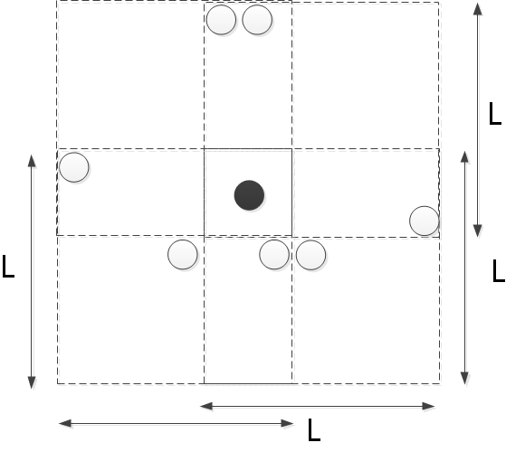
Figure II.1: This figure presents an example for a set of 8 points that cannot be decomposed into 4 non-intersecting subsets that meet the separation condition as in (I.7), although each resolution cell contains at most 4 points. Consider a square resolution cell (in $\ell_{\infty}$ sense) of size $L\times L$. Note that indeed each resolution cell contains at most 4 points. Nonetheless, this set of points cannot be described as 4 non-intersecting sets that satisfy the separation condition. Specifically, the distance (in $\ell_{\infty}$ norm) of the black point is smaller than $L$ from the other 7 points, meaning it has to be in a separate subset from the others. On the other hand, there is no triplet of points that comprises a legal subset. Therefore, the property of Definition II.6 is not a consequence of the two-dimensional version of Definition II.1.

A two-dimensional non-negative admissible kernel is defined as follows:

Definition II.7.

We say that $\mathbf{g_{2}}$ is a two-dimensional non-negative admissible kernel if $\mathbf{g_{2}}\left(t_{1},t_{2}\right)\geq 0$ for all $\left(t_{1},t_{2}\right)\in\mathbb{R}^{2}$ and it has the following properties:

1. $\mathbf{g_{2}}\in\mathcal{C}^{3}\left(\mathbb{R}^{2}\right)$ and

   $$\mathbf{g_{2}}\left(t_{1},t_{2}\right)=\mathbf{g_{2}}\left(-t_{1},t_{2}\right)=\mathbf{g_{2}}\left(t_{1},-t_{2}\right)=\mathbf{g_{2}}\left(-t_{1},-t_{2}\right).$$

2. Global property: There exist constants $C_{\ell_{1},\ell_{2}}>0$ such that $\left|\mathbf{g_{2}}^{(\ell_{1},\ell_{2})}\left(t_{1},t_{2}\right)\right|\leq\frac{C_{\ell_{1},\ell_{2}}}{\left(1+t_{1}^{2}+t_{2}^{2}\right)^{3/2}}$, for $\ell_{1}+\ell_{2}\leq 3$, where $\mathbf{g_{2}}^{(\ell_{1},\ell_{2})}\left(t_{1},t_{2}\right):=\frac{\partial^{\ell_{1}}\partial^{\ell_{2}}}{\partial t_{1}^{\ell_{1}}\partial t_{2}^{\ell_{2}}}\mathbf{g_{2}}\left(t_{1},t_{2}\right)$.

3. Local property: There exist constants $\beta,\varepsilon>0$ such that

   1. $\mathbf{g_{2}}\left(t_{1},t_{2}\right)<\mathbf{g_{2}}(\varepsilon,0)$ for all $\left(t_{1},t_{2}\right)$ satisfying $|t_{1}|>\varepsilon$, and $\mathbf{g_{2}}\left(t_{1},t_{2}\right)<\mathbf{g_{2}}(0,\varepsilon)$ for all $\left(t_{1},t_{2}\right)$ satisfying $|t_{2}|>\varepsilon$.

   2. $\mathbf{g_{2}}^{(2,0)}\left(t_{1},t_{2}\right),\mathbf{g_{2}}^{(0,2)}\left(t_{1},t_{2}\right)<-\beta$ for all $\left(t_{1},t_{2}\right)$ satisfying $|t_{1}|,|t_{2}|\leq\epsilon$.

Equipped with the appropriate definitions of Rayleigh regularity and non-negative admissible kernel, we are ready to state our main theorem for the two-dimensional case. The theorem is proved in Section IV.

Theorem II.8.

Consider the model (I) for a non-negative two-dimensional admissible kernel $\mathbf{g_{2}}$ as defined in Definition II.7. Then, there exists $\nu>0$ such that if $\mathcal{\mbox{supp$\left(\mathbf{x_{2}}\right)$}}\in\mathcal{R}_{2}^{idx}\left(\nu\sigma,r\right)$, the solution $\hat{\mathbf{x}}_{\mathbf{2}}$ of the convex problem

$$\min_{\tilde{\mathbf{x}}}\quad\left\|\tilde{\mathbf{x}}\right\|_{1}\quad\mbox{subject to}\quad\left\|\mathbf{y}-\mathbf{g_{2}}\ast\tilde{\mathbf{x}}\right\|_{1}\leq\delta,\thinspace\tilde{\mathbf{x}}\geq 0,$$ (II.5)

satisfies (for sufficiently large $N$ and $\nu$)

$$\left\|\hat{\mathbf{x}}_{\mathbf{2}}-\mathbf{x_{2}}\right\|_{1}\leq C_{2}\left(\mathbf{g_{2}},r\right)\left(N\sigma\right)^{2r}\delta,$$

where $C_{2}\left(\mathbf{g_{2}},r\right)$ is a constant which depends on the kernel $\mathbf{g_{2}}$ and the Rayleigh regularity $r$.

To conclude this section, we summarize the contribution of this paper and compare it to the relevant previous works. Particularly, we stress the chief differences from [39, 12] which served as inspiration for this work.

• This work deviates from [39] in two important aspects. First, our stability results is much stronger than those in [39]. Particularly, our main results hold for signals with $r$ spikes within a resolution cell. In contrast, the main theorems of [39] require signals with $r$ spikes within $r$ resolution cells. Second, our formulation is not restricted to kernels with finite bandwidth and, in this manner, can be seen as a generalization of [39]. This generalization is of particular interest as many kernels in practical applications are not band-limited.

• In [12], it is proven that robust recovery from general stream of pulses (not necessarily non-negative) is possible if the delays are not clustered. Here, we show that the separation is unnecessary in the positive case and can be replaced by the notion of Raleigh regularity. This notion quantifies the density of the signal’s support.

• We derive strong stability guarantees compared to parametric methods, such as Prony method, matrix pencil and MUSIC. Nevertheless, we heavily rely on the positiveness of signal and the density of the delays, whereas the parametric methods do not have these restrictions. We also mention that several previous works suggested noise-free results for non-negative signals in similar settings, however they do not derive stability guarantees [31, 40, 41, 42]. In [43] it was proven that the necessary separation between the delays drops to zero for sufficiently low noise level.

III Proof of Theorem II.4

The proof follows the outline of [39] and borrows constructions from [12]. Let $\hat{\mathbf{x}}$ be s solution of (II.2) and set $\mathbf{h}:=\hat{\mathbf{x}}-\mathbf{x}$. Observe that by (II.2) $\left\|\mathbf{h}\right\|_{1}$ is finite since $\left\|\mathbf{h}\right\|_{1}\leq\left\|\hat{\mathbf{x}}\right\|_{1}+\left\|\mathbf{x}\right\|_{1}\leq 2\left\|\mathbf{x}\right\|_{1}$. The proof relies on some fundamental results from [12] (particularly, see Proposition 3.3 and Lemmas 3.4 and 3.5) which are summarized by the following lemma:

Lemma III.1.

Let $\mathbf{g}$ be a non-negative admissible kernel as defined in Definition II.3 and suppose that $\mathcal{T}:=\left\{t_{m}\right\}\in\mathcal{R}^{idx}\left(\nu\sigma,1\right)$. Then, there exists a kernel-dependent separation constant $\nu>0$ (see (I.6)) and a set of coefficients $\left\{a_{m}\right\}$ and $\left\{b_{m}\right\}$ such there exists an associated function of the form

$$\tilde{\mathbf{q}}(t)=\sum_{m}a_{m}\mathbf{g}\left(\frac{t-t_{m}}{\sigma}\right)+b_{m}\mathbf{g}^{(1)}\left(\frac{t-t_{m}}{\sigma}\right),$$ (III.1)

which satisfies:

$$\tilde{\mathbf{q}}\left(t_{m}\right) = 1,\quad t_{m}\in\mathcal{T},$$

$$\tilde{\mathbf{q}}\left(t\right) \leq 1-\frac{\beta\left(t-t_{m}\right)^{2}}{4\mathbf{g}(0)\sigma^{2}},\quad\left|t-t_{m}\right|\leq\varepsilon\sigma,\thinspace t_{m}\in\mathcal{T},$$

$$\tilde{\mathbf{q}}\left(t\right) < 1-\frac{\beta\varepsilon^{2}}{4\mathbf{g}(0)},\quad\left|t-t_{m}\right|>\varepsilon\sigma,\thinspace\forall t_{m}\in\mathcal{T},$$

$$\tilde{\mathbf{q}}\left(t\right) \geq 0,\quad t\in\mathbb{R},$$

where $\varepsilon$ and $\beta$ are the constants associated with $\mathbf{g}$. Furthermore,

$$\left\|\mathbf{a}\right\|_{\infty} := \underset{m}{\max}\left|a_{m}\right|\leq\frac{3\nu^{2}}{3\mathbf{g}\left(0\right)\nu^{2}-2\pi^{2}C_{0}},$$ (III.2)

$$\left\|\mathbf{b}\right\|_{\infty} := \underset{m}{\max}\left|b_{m}\right|$$

$$\leq \frac{\pi^{2}C_{1}}{\left(3\left|\mathbf{g}^{\left(2\right)}\left(0\right)\right|\nu^{2}-\pi^{2}C_{2}\right)\left(3\mathbf{g}\left(0\right)\nu^{2}-2\pi^{2}C_{0}\right)}.$$

Remark III.2.

The non-negativity property, $\tilde{\mathbf{q}}\left(t\right)\geq 0$ for all $t\in\mathbb{R}$, does not appear in [12], however, it is a direct corollary of the non-negativity assumption that $\mathbf{g}(t)\geq 0$ for all $t\in\mathbb{R}$.

The interpolating function (III.1) also satisfies the following property which will be needed in the proof:

Lemma III.3.

Let $\hat{\mathbf{x}}$ be s solution of (II.2) and set $\mathbf{h}:=\hat{\mathbf{x}}-\mathbf{x}$. Let $\left\{\mathcal{T}_{i}\right\}_{i=1}^{r}$ be a union of $r$ non-intersecting sets obeying $\mathcal{T}_{i}\in\mathcal{R}^{idx}\left(\nu\sigma,1\right)$ for all $i\in\left\{1,\dots,r\right\}$. For each set $\mathcal{T}_{i}$, let $\tilde{\mathbf{q}}_{i}[k]:=\tilde{\mathbf{q}}_{i}\left(k/N\right)$, $k\in\mathbb{Z}$, be an associated function, where $\tilde{\mathbf{q}_{i}}(t)$ is given in (III.1). Then, for any sequence $\left\{\alpha_{i}\right\}_{i=1}^{r}\in\left\{0,1\right\}$ we have

$$\begin{split}&\sum_{k\in\mathbb{Z}}\prod_{i=1}^{r}\left(\tilde{\mathbf{q}}_{i}\left[k\right]\right)^{\alpha_{i}}\mathbf{h}[k]\\ &\leq\left(C_{0}\left(1+\frac{\pi^{2}}{6\nu^{2}}\right)\right)^{r-1}\left(\frac{6\nu^{2}}{3\mathbf{g}\left(0\right)\nu^{2}-2\pi^{2}C_{0}}\right)^{r}\delta\\ &+c^{*}\nu^{-4}\left\|\mathbf{h}\right\|_{1},\end{split}$$ (III.4)

for some constant $c^{*}>0$ that depends on the kernel $\mathbf{g}$.

Proof.

We begin by two preliminary calculations. First, we observe from (I.3) and (II.2) that

$$\sum_{n\in\mathbb{Z}}\left|\sum_{k\in\mathbb{Z}}\mathbf{g}\left[k-n\right]\mathbf{h}[k]\right| \leq \left\|\mathbf{y}-\mathbf{g}\ast\hat{\mathbf{x}}\right\|_{1}$$ (III.5)

$$+ \left\|\mathbf{g}\ast\mathbf{x}-\mathbf{y}\right\|_{1}$$

$$\leq 2\delta.$$

Additionally, we can estimate for all $k\in\mathbb{Z}$ (see Section 3.4 in [12])

$$\sum_{k_{m}\in\mathcal{T}_{i}}\frac{1}{1+\left(\frac{k-k_{m}}{N\sigma}\right)^{2}}<2\left(1+\frac{\pi^{2}}{6\nu^{2}}\right),$$

and hence with the properties of admissible kernel as defined in Definition II.3 we have for $\ell=0,1,$

$$\left|\sum_{k_{m}\in\mathcal{T}_{i}}\mathbf{g}^{(\ell)}\left[k-k_{m}\right]\right| \leq C_{\ell}\sum_{k_{m}\in\mathcal{T}_{i}}\frac{1}{1+\left(\frac{k-k_{m}}{N\sigma}\right)^{2}}$$ (III.6)

$$\leq 2C_{\ell}\left(1+\frac{\pi^{2}}{6\nu^{2}}\right).$$

According to (III.1), the left-hand of (III.4) can be explicitly written as:

$$\begin{split}&\sum_{k\in\mathbb{Z}}\prod_{i=1}^{r}\left(\tilde{\mathbf{q}}_{i}\left[k\right]\right)^{\alpha_{i}}\mathbf{h}[k]\\ &=\sum_{k\in\mathbb{Z}}\prod_{i=1}^{r}\left(\sum_{k_{m_{i}}\in\mathcal{T}_{i}}a_{m_{i}}\mathbf{g}\left[k-k_{m_{i}}\right]+b_{m_{i}}\mathbf{g}^{(1)}\left[k-k_{m_{i}}\right]\right)^{\alpha_{i}}\mathbf{h}[k].\end{split}$$ (III.7)

This expression can be decomposed into (at most) $2^{r}$ terms. We commence by considering the first term of the expression with $\alpha_{1}=\alpha_{2}=1$ and $\alpha_{i}=0$ for $i>2$ (namely, the product of the shifts of $\mathbf{g}$). Using (III.5) and (III.6) we get

$$\sum_{k\in\mathbb{Z}}\sum_{k_{m_{1}}\in\mathcal{T}_{1}}a_{m_{1}}\mathbf{g}\left[k-k_{m_{1}}\right]\sum_{k_{m_{2}}\in\mathcal{T}_{2}}a_{m_{2}}\mathbf{g}\left[k-k_{m_{2}}\right]\mathbf{h}[k]$$

$$\leq \left\|\mathbf{a}\right\|_{\infty}^{2}\left|\sum_{{}_{k_{m_{1}}\in\mathcal{T}_{1}}}\sum_{k\in\mathbb{Z}}\mathbf{g}\left[k-k_{m_{1}}\right]\mathbf{h}[k]\sum_{k_{m_{2}}\in\mathcal{T}_{2}}\mathbf{g}\left[k-k_{m_{2}}\right]\right|$$

$$\leq 2\left\|\mathbf{a}\right\|_{\infty}^{2}C_{0}\left(1+\frac{\pi^{2}}{6\nu^{2}}\right)\sum_{n\in\mathbb{Z}}\left|\sum_{k\in\mathbb{Z}}\mathbf{g}\left[k-n\right]\mathbf{h}[k]\right|$$

$$\leq 4\left\|\mathbf{a}\right\|_{\infty}^{2}C_{0}\left(1+\frac{\pi^{2}}{6\nu^{2}}\right)\delta.$$

From the same methodology and using (III.2), we conclude that for any sequence of coefficients $\left\{\alpha_{i}\right\}_{i=1}^{r}\in\left\{0,1\right\}$ we get

$$\begin{split}&\sum_{k\in\mathbb{Z}}\prod_{i=1}^{r}\left(\sum_{k_{m_{i}}\in\mathcal{T}_{i}}a_{m_{i}}\mathbf{g}\left[k-k_{m_{i}}\right]\right)\mathbf{h}[k]\\ &\leq\left(C_{0}\left(1+\frac{\pi^{2}}{6\nu^{2}}\right)\right)^{r-1}\left(\frac{6\nu^{2}}{3\mathbf{g}\left(0\right)\nu^{2}-2\pi^{2}C_{0}}\right)^{r}\delta.\end{split}$$

Next, using (III.6) we observe that all other $2^{r}-1$ terms of (III.7) can be bounded by $c_{0}\left\|\mathbf{a}\right\|_{\infty}^{\beta_{1}}\left\|\mathbf{b}\right\|_{\infty}^{\beta_{2}}\left\|\mathbf{h}\right\|_{1}$ for some constant $c_{0}>0$ and $0\leq\beta_{1}\leq r-1$, $1\leq\beta_{2}\leq r$. Hence, we conclude by (III.2) and (III.1) that the summation of all these terms is bounded by $c^{*}\nu^{-4}\left\|\mathbf{h}\right\|_{1}$ for sufficiently large constants $c^{*}>0$ and $\nu$. The constant $c^{*}>0$ depends only on the kernel $\mathbf{g}$. This completes the proof. ∎

Consider $\mathbf{x}\in\mathcal{R}_{+}\left(\nu\sigma,r\right)$ and let us define the sets $\mathcal{N}:=\left\{k/N\thinspace:\thinspace\mathbf{h}[k]<0\right\}$ and respectively $\mathcal{N}^{C}:=\left\{k/N\thinspace:\thinspace\mathbf{h}[k]\geq 0\right\}$. Throughout the proof, we use the notation $k\in\mathcal{N}$ and $k\in\mathcal{N}^{C}$ to denote some $k\in\mathbb{Z}$ so that $k/N\in\mathcal{N}$ and $k/N\in\mathcal{N}^{C}$, respectively. Observe that by definition, $\mathcal{N}\subseteq\mbox{supp}(\mathbf{x})$ and thus $\mathcal{N}\in\mathcal{R}^{idx}\left(\nu\sigma,r\right)$. The set $\mathcal{N}$ can be presented as the union of $r$ non-intersecting subsets $\mathcal{N}=\cup_{i=1}^{r}\mathcal{N}_{i}$, where $\mathcal{N}_{i}=\left\{t_{i},t_{i+r},t_{i+2r},\dots\right\}$ and $\mathcal{N}_{i}\in\mathcal{R}^{idx}\left(\nu\sigma,1\right)$. Therefore, for each subset $\mathcal{N}_{i}$ there exists an associated function $\tilde{\mathbf{q}}_{i}[k]=\tilde{\mathbf{q}}_{i}\left(k/N\right)$ as given in Lemma III.1. The proof builds upon the following construction

$$\mathbf{q}[k]:=\prod_{i=1}^{r}\left(1-\tilde{\mathbf{q}}_{i}[k]\right)-\rho,$$ (III.8)

for some constant $\rho>0$, to be defined later. The function $\mathbf{q}[k]$ satisfies the following properties:

Lemma III.4.

Let $\mathbf{q}$ be as in (III.8), let $N\sigma>\left(\frac{1}{2}\right)^{\frac{1}{2r}+1}\sqrt{\frac{\beta}{\mathbf{g}(0)}}$ and let

$$\rho\geq\frac{1}{2}\left(\frac{\beta}{4\mathbf{g}(0)\gamma^{2}}\right)^{r},$$ (III.9)

where $\gamma:=\max\left\{N\sigma,\varepsilon^{-1}\right\}$. Then, we have

$$\mathbf{q}\left[k_{m}\right] = -\rho,\quad k_{m}\in\mathcal{N},$$

$$\mathbf{q}\left[k\right] \geq \rho,\quad k\in\mathcal{N}^{C},$$

$$\mathbf{q}\left[k\right] \leq 1,\quad k\in\mathbb{Z}.$$

Proof.

Since $\mathcal{N}_{i}\in\mathcal{R}^{idx}\left(\nu\sigma,1\right),$ by Lemma III.1 there exists for each subset $\mathcal{N}_{i}$ an associated interpolating function $\tilde{\mathbf{q}_{i}}[k]=\tilde{\mathbf{q}_{i}}(k/N)$. Consequently, for all $k_{m}\in\mathcal{N}$ we obtain

$$\begin{split}\mathbf{q}\left[k_{m}\right]&=\prod_{i=1}^{r}\left(1-\tilde{\mathbf{q}}_{i}\left[k_{m}\right]\right)-\rho\\ &=-\rho,\end{split}$$

and for all $k\in\mathcal{N}^{C}$ we have

$$\mathbf{q}[k] = \prod_{i=1}^{r}\left(1-\tilde{\mathbf{q}}_{i}\left[k\right]\right)-\rho$$

$$\geq \left(\frac{\beta}{4\mathbf{g}(0)\gamma^{2}}\right)^{r}-\rho.$$

By setting

$$\rho:=\arg\min_{k\in\mathcal{N}^{C}}\mathbf{q}[k]\geq\frac{1}{2}\left(\frac{\beta}{4\mathbf{g}(0)\gamma^{2}}\right)^{r},$$

we conclude the proof. Note that in order to guarantees $\rho<1$, we require $N\sigma>\left(\frac{1}{2}\right)^{\frac{1}{2r}+1}\sqrt{\frac{\beta}{\mathbf{g}(0)}}$ . ∎

Equipped with Lemma III.4, we conclude that $\mathbf{q}[k]$ and $\mathbf{h}[k]$ have the same sign for all $k\in\mathbb{Z}$, and thus

$$\begin{split}\left\langle\mathbf{q},\mathbf{h}\right\rangle=\sum_{k\in\mathbb{Z}}\mathbf{q}[k]\mathbf{h}[k]&=\sum_{k\in\mathbb{Z}}|\mathbf{q}[k]||\mathbf{h}[k]|\\ &\geq\rho\left\|\mathbf{h}\right\|_{1}.\end{split}$$ (III.10)

To complete the proof, we need to bound the inner product $\left\langle\mathbf{q},\mathbf{h}\right\rangle$ from above. To this end, observe that

$$\prod_{i=1}^{r}\left(1-\tilde{\mathbf{q}}_{i}\left[k\right]\right)=1+\boldsymbol{\kappa}_{r}[k],$$ (III.11)

where

$$\boldsymbol{\kappa}_{r}[k] := \sum_{j=1}^{2^{r}-1}\prod_{i=1}^{r}\left(-\tilde{\mathbf{q}}_{i}\left[k\right]\right)^{\alpha_{i}(j)},$$ (III.12)

for some coefficients $\left\{\alpha_{i}(j)\right\}_{i=1}^{r}\in\left\{0,1\right\}$. For instance, $\boldsymbol{\kappa}_{2}[k]=-\tilde{\mathbf{q}}_{1}\left[k\right]-\tilde{\mathbf{q}}_{2}\left[k\right]+\tilde{\mathbf{q}}_{1}\left[k\right]\tilde{\mathbf{q}}_{2}\left[k\right].$ Therefore, by (III.8) and (III.11) we get

$$\left\langle\mathbf{q},\mathbf{h}\right\rangle = \left\langle\prod_{i=1}^{r}\left(1-\tilde{\mathbf{q}}_{i}\left[k\right]\right)-\rho,\mathbf{h}\right\rangle$$

$$= \left\langle\left(1-\rho\right)+\boldsymbol{\kappa}_{r},\mathbf{h}\right\rangle$$

$$= \left(1-\rho\right)\sum_{k\in\mathbb{Z}}\mathbf{h}[k]+\left\langle\boldsymbol{\kappa}_{r},\mathbf{h}\right\rangle.$$

Recall that by (II.2) we have $\left\|\hat{\mathbf{x}}\right\|_{1}\leq\left\|\mathbf{x}\right\|_{1}$ and therefore

$$\begin{split}\left\|\mathbf{x}\right\|_{1}\geq\left\|\mathbf{x}+\mathbf{h}\right\|_{1}&=\sum_{k\in\mbox{supp}(\mathbf{x})}\left|\mathbf{x}[k]+\mathbf{h}[k]\right|\\ &+\sum_{k\in\mathbb{Z}\backslash\mbox{supp}(\mathbf{x})}\left|\mathbf{h}[k]\right|.\end{split}$$

By definition $\mathbf{h}[k]\geq 0$ for all $k\in\mathcal{N}^{C}$ and we use the triangle inequality to deduce

$$\left\|\mathbf{x}\right\|_{1} \geq \sum_{k\in\mathbb{Z}\backslash\mbox{supp}(\mathbf{x})}\mathbf{h}[k]$$

$$+ \sum_{k\in\mbox{supp}(\mathbf{x})\backslash\mathcal{N}}\left(\mathbf{x}[k]+\mathbf{h}[k]\right)+\sum_{k\in\mathcal{N}}\left|\mathbf{x}[k]+\mathbf{h}[k]\right|$$

$$\geq \left\|\mathbf{x}\right\|_{1}+\sum_{k\in\mathcal{N}^{C}}\mathbf{h}[k]-\sum_{k\in\mathcal{N}}\left|\mathbf{h}[k]\right|,$$

and thus we conclude

$$\sum_{k\in\mathbb{Z}}\mathbf{h}[k]\leq 0.$$ (III.14)

So, from (III.12), (III), (III.14) and Lemma III.3 we conclude that

$$\left\langle\mathbf{q},\mathbf{h}\right\rangle \leq \left|\left\langle\boldsymbol{\boldsymbol{\kappa}}_{r},\mathbf{h}\right\rangle\right|\leq\sum_{j=1}^{2^{r}-1}\left|\sum_{k\in\mathbb{Z}}\prod_{i=1}^{r}\left(\tilde{\mathbf{q}}_{i}\left[k\right]\right)^{\alpha_{i}(j)}\mathbf{h}[k]\right|$$ (III.15)

$$\leq \left(2^{r}-1\right)\left(C_{0}\left(1+\frac{\pi^{2}}{6\nu^{2}}\right)\right)^{r-1}$$

$$\cdot \left(\frac{6\nu^{2}}{3\mathbf{g}\left(0\right)\nu^{2}-2\pi^{2}C_{0}}\right)^{r}\delta$$

$$+ c^{*}\left(2^{r}-1\right)\nu^{-4}\left\|\mathbf{h}\right\|_{1}.$$

Combining (III.15) with (III.10) and (III.9) yields

$$\left\|\mathbf{h}\right\|_{1} \leq \frac{\left(2^{r}-1\right)\left(C_{0}\left(1+\frac{\pi^{2}}{6\nu^{2}}\right)\right)^{r-1}\left(\frac{6\nu^{2}}{3\mathbf{g}\left(0\right)\nu^{2}-2\pi^{2}C_{0}}\right)^{r}}{\frac{1}{2}\left(\frac{\beta}{4\mathbf{g}(0)\gamma^{2}}\right)^{r}-c^{*}\left(2^{r}-1\right)\nu^{-4}}\delta.$$

This completes the proof of Theorem II.4.

IV Proof of Theorem II.8

The proof of Theorem II.8 follows the methodology of the proof in Section III. We commence by stating the extension of Lemma III.1 to the two-dimensional case, based on results from [12]:

Lemma IV.1.

Let $\mathbf{g_{2}}$ be a non-negative two-dimensional admissible kernel as defined in Definition II.3 and suppose that $\mathcal{T}_{2}:=\left\{\mathbf{t}_{m}\right\}\in\mathcal{R}_{2}^{idx}\left(\nu\sigma,1\right)$. Then, there exists a kernel-dependent separation constant $\nu>0$ and a set of coefficients $\left\{a_{m}\right\},\left\{b_{m}^{1}\right\}$ and $\left\{b_{m}^{2}\right\}$ such that there exist an associated function of the form

$$\begin{split}\mathbf{q_{2}}(\mathbf{t})=\sum_{m}a_{m}\mathbf{g_{2}}\left(\frac{\mathbf{t}-\mathbf{t}_{m}}{\sigma}\right)&+b_{m}^{1}\mathbf{g_{2}}^{(1,0)}\left(\frac{\mathbf{t}-\mathbf{t}_{m}}{\sigma}\right)\\ &+b_{m}^{2}\mathbf{g_{2}}^{(0,1)}\left(\frac{\mathbf{t}-\mathbf{t}_{m}}{\sigma}\right),\end{split}$$ (IV.1)

which satisfies:

$$\tilde{\mathbf{q}}_{\mathbf{2}}\left(\mathbf{t}\right) = 1,\quad{t}_{m}\in\mathcal{T}_{2},$$

$$\tilde{\mathbf{q}}\left(\mathbf{t}\right) \leq 1-c_{1}\frac{\left\|\mathbf{t}-\mathbf{t}_{m}\right\|_{2}^{2}}{\sigma^{2}},\left\|\mathbf{t}-\mathbf{t}_{m}\right\|_{\infty}\leq\sigma\varepsilon_{1},\thinspace\mathbf{t}_{m}\in\mathcal{T}_{2},$$

$$\tilde{\mathbf{q}}\left(\mathbf{t}\right) \leq 1-c_{2},\quad\left\|\mathbf{t}-\mathbf{t}_{m}\right\|_{\infty}>\varepsilon_{1}\sigma,\thinspace\forall\mathbf{t}_{m}\in\mathcal{T}_{2},$$

$$\tilde{\mathbf{q}}\left(\mathbf{t}\right) \geq 0,$$

for sufficiently small $\varepsilon_{1}\leq\varepsilon$ associated with the kernel $\mathbf{g_{2}}$, and some constants $c_{1},c_{2}>0$. For sufficiently large $\nu>0$ and constants $c_{a},c_{b}>0$, we also have

$$\left\|\mathbf{a}\right\|_{\infty}: = \underset{m}{\max}\left|a_{m}\right|\leq\frac{1}{\mathbf{g_{2}}(0,0)}+c_{a}\nu^{-3},$$

$$\left\|\mathbf{\tilde{b}}\right\|_{\infty}: = \underset{m}{\max}\left|b_{m}^{1}\right|,\left|b_{m}^{2}\right|\leq c_{b}\nu^{-6}.$$

We present now the two-dimensional version of Lemma III.3 without a proof. The proof relies on the same methodology as the one-dimensional case.

Lemma IV.2.

Let $\left\{\mathcal{T}_{i,2}\right\}_{i=1}^{r}$ be a union of $r$ non-intersecting sets obeying $\mathcal{T}_{i,2}\in\mathcal{R}_{2}^{idx}\left(\nu\sigma,1\right)$ for all $i\in\left\{1,\dots,r\right\}$. For each set $\mathcal{T}_{i,2}$, let $\tilde{\mathbf{q}}_{\mathbf{i,2}}[\mathbf{k}]:=\tilde{\mathbf{q}}_{\mathbf{i,2}}\left(\mathbf{k}/N\right)$, $\mathbf{k}\in\mathbb{Z}^{2}$, be an associated function, where $\tilde{\mathbf{q}}_{\mathbf{i,2}}(\mathbf{t})$ is given in (IV.1). Then, for any sequence $\left\{\alpha_{i}\right\}_{i=1}^{r}\in\left\{0,1\right\}$ we have for sufficiently large $\nu$,

$$\sum_{{k}\in\mathbb{Z}^{2}}\prod_{i=1}^{r}\left(\tilde{\mathbf{q}}_{\mathbf{i,2}}\left[{k}\right]\right)^{\alpha_{i}}\mathbf{h}[{k}]\leq\tilde{C}_{2}(\mathbf{g},r)\delta+c^{*}\nu^{-6}\left\|\mathbf{h}\right\|_{1},$$ (IV.2)

for some constants $c^{*}>0$ and $\tilde{C}_{2}(\mathbf{g_{2}},r)$ which depends on the kernel $\mathbf{g_{2}}$ and the regularity parameter $r$.

Let $\mathbf{k}\in\mathbb{Z}^{2}$. Let us define the sets $\mathcal{N}_{2}:=\left\{\mathbf{k}/N\thinspace:\thinspace\mathbf{h}[\mathbf{k}]<0\right\}$ and $\mathcal{N}_{2}^{C}:=\left\{\mathbf{k}/N\thinspace:\thinspace\mathbf{h}[\mathbf{k}]\geq 0\right\}$. Throughout the proof, we use the notation of $\mathbf{k}\in\mathcal{N}_{2}$ and $\mathbf{k}\in\mathcal{N}_{2}^{C}$ to denote all $\mathbf{k}\in\mathbb{Z}^{2}$ so that $\mathbf{k}/N\in\mathcal{N}_{2}$ and $\mathbf{k}/N\in\mathcal{N}_{2}^{C}$, respectively. By definition, $\mathcal{N}_{2}\in\mathcal{R}_{2}^{idx}\left(\nu\sigma,r\right)$ (see Definition II.6) and it can be presented as the union of non-intersecting subsets $\mathcal{N}_{2}=\cup_{i=1}^{r}\mathcal{N}_{i,2}$ where $\mathcal{N}_{i,2}\in\mathcal{R}_{2}^{idx}\left(\nu\sigma,1\right)$. Therefore, for each subset $\mathcal{N}_{i,2}$ there exists an associated function $\tilde{\mathbf{q}}_{\mathbf{i,2}}[\mathbf{k}]=\tilde{\mathbf{q}}_{\mathbf{i,2}}\left(\mathbf{k}/N\right)$ given in Lemma IV.1. As in the one-dimensional case, the proof relies on the following construction

$$\mathbf{q_{2}}[\mathbf{k}]:=\prod_{i=1}^{r}\left(1-\tilde{\mathbf{q}}_{\mathbf{i,2}}[\mathbf{k}]\right)-\rho,$$ (IV.3)

for some constant $\rho>0$, to be defined later. This function satisfies the following interpolation properties:

Lemma IV.3.

Suppose that

$$N\sigma>\max\left\{\sqrt{\frac{c_{1}}{c_{2}}},\left(\varepsilon_{1}\right)^{-1},\left(\frac{1}{2}\right)^{\frac{1}{2r}}\sqrt{c_{1}}\right\},$$

where $\varepsilon_{1}$ is given in Lemma IV.1. Let $\mathbf{q_{2}}$ be as in (IV.3) and let

$$\rho\geq\frac{1}{2}\left(\frac{c_{1}}{\left(N\sigma\right)^{2}}\right)^{r}.$$ (IV.4)

Then,

$$\mathbf{q_{2}}\left[\mathbf{k}_{m}\right] = -\rho,\quad\mathbf{k}_{m}\in\mathcal{N}_{2},$$

$$\mathbf{q_{2}}\left[\mathbf{k}\right] \geq \rho,\quad\mathbf{k}\in\mathcal{N}_{2}^{C},$$

$$\mathbf{q_{2}}\left[\mathbf{k}\right] \leq 1,\quad\mathbf{k}\in\mathbb{Z}^{2}.$$

Proof.

Since $\mathcal{N}_{i,2}\in\mathcal{R}_{2}^{idx}\left(\nu\sigma,1\right),$ by Lemma IV.1 there exists for each subset $\mathcal{N}_{i,2}$ an associated function $\tilde{\mathbf{q}}_{\mathbf{i,2}}[{k}]=\tilde{\mathbf{q}}_{\mathbf{i,2}}(\mathbf{k}/N)$. Consequently, for all $\mathbf{k}_{m}\in\mathcal{N}_{2}$ we obtain

$$\mathbf{q_{2}}\left[\mathbf{k}_{m}\right]=\prod_{i=1}^{r}\left(1-\mathbf{q_{i,2}}\left[\mathbf{k}_{m}\right]\right)-\rho=-\rho.$$

For $N\sigma\geq\max\left\{\sqrt{\frac{c_{1}}{c_{2}}},\left(\varepsilon_{1}\right)^{-1}\right\}$ we get for all $\mathbf{k}\in\mathcal{N}_{2}^{C}$

$$\mathbf{q_{2}}[\mathbf{k}] = \prod_{i=1}^{r}\left(1-\mathbf{q_{i,2}}\left[\mathbf{k}\right]\right)-\rho\geq\left(\frac{c_{1}}{\left(N\sigma\right)^{2}}\right)^{r}-\rho.$$

By setting

$$\rho:=\arg\min_{\mathbf{k}\in\mathcal{N}_{2}^{C}}\mathbf{q_{2}}[\mathbf{k}]\geq\frac{1}{2}\left(\frac{c_{1}}{\left(N\sigma\right)^{2}}\right)^{r},$$

we conclude the proof. The condition $N\sigma>\left(\frac{1}{2}\right)^{\frac{1}{2r}}\sqrt{c_{1}}$ guarantees that $\rho<1$. ∎

Once we constructed the function $\mathbf{q_{2}}[\mathbf{k}]$, the proof follows the one-dimensional case. By considering Lemmas IV.2 and IV.3 and using similar arguments to (III.10) and (III.15), we conclude

$$\begin{split}\rho\left\|\mathbf{h}\right\|_{1}&\leq\left\langle\mathbf{q},\mathbf{h}\right\rangle\leq\left(3^{r}-1\right)\tilde{C}_{2}(\mathbf{g}_{2},r)\delta\\ &+c^{*}\left(3^{r}-1\right)\nu^{-6}\left\|\mathbf{h}\right\|_{1}.\end{split}$$

Using (IV.4) we get for sufficiently large $\nu$ that

$$\left\|\mathbf{h}\right\|_{1}\leq C_{2}\left(\mathbf{g}_{2},r\right)\left(N\sigma\right)^{2r}\delta,$$

for some constant ${C}_{2}(\mathbf{g}_{2},r)$ which depends on the kernel $\mathbf{g}_{2}$ and the Rayleigh regularity $r$.

V Numerical Experiments

We conducted numerical experiments to validate the theoretical results of this paper. The simulated signals were generated in two steps. First, random locations were sequentially added to the signal’s support in the interval $[-1,1]$ with discretization step of 0.01, while keeping a fixed regularity condition. Once the support was determined, the amplitudes were drawn randomly from an i.i.d normal distribution with standard deviation SD = 10. For positive signals, the amplitudes are taken to be the absolute values of the normal variables.

The experiments were conducted with the Cauchy kernel $\mathbf{g}(t)=\frac{1}{1+\left(\frac{t}{\sigma}\right)^{2}}$, $\sigma=0.1$. We set the separation constant to be $\nu=0.5$, which was evaluated in [12] to be the minimal separation constant, guaranteeing the existence of interpolating polynomial as in Lemma III.1. Figure V.1 presents an example for the estimation of the signal (I.2) from (I.3) with $r=2$. As can be seen, the solution of the convex problem (II.2) detects the support of the signal with high precision in a noisy environment of $27$ dB. Figure V.2 presents an example for recovery of a two-dimensional signal from a stream of Cauchy kernels with $r=2$ and $\nu=0.8$.

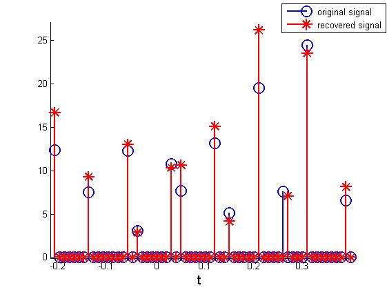
Figure V.1: Example for the recovery of a signal of the form of (I.2) from stream of Cauchy kernels with $\sigma=0.1$, Rayleigh regularity of $r=2$, separation constant of $\nu=0.5$ and noise level of $\delta=75$ (SNR=27dB).

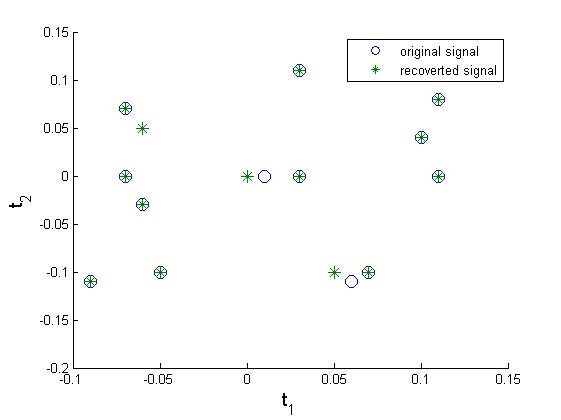
Figure V.2: An example for the recovery of a two-dimensional signal of the form (I.5) from the measurements (I), with $r=2$, $\delta=400$ and $\nu=0.8$. The figure presents merely the locations (support) of the original and the recovered signals.

Figure V.3 shows the localization error as a function of the noise level $\delta$. To clarify, by localization error we mean the distance between the support of the original signal and the support of the recovered signal. Figure V.3a compares the localization error for positive signals and general real signals (i.e. not necessarily positive) from stream of Cauchy pulses. For general signals, we solved a standard $\ell_{1}$ minimization problem as in [12], which is the same problem as (II.2) without the positivity constraint $\mathbf{x}\geq 0$. Plainly, the localization error of positive signals is significantly smaller than the error of general signals. Figure V.3b shows that the error grows approximately linearly with the noise level $\delta$ and increases with $r$.

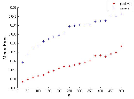
(a) Mean localization error of positive signal and general signal (not necessarily positive coefficients) with $r=2.$

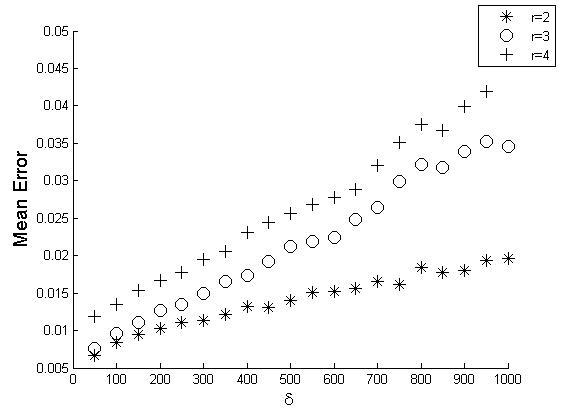
(b) Mean localization error of positive signals for $r=2,3,4$.

Figure V.3: Mean localization error from a stream of Cauchy pulses as a function of the noise level $\delta$. For each value of $\delta,$ 50 experiments were conducted.

VI Conclusions

In this paper, we have shown that a standard convex optimization program can robustly recover the sets of delays and positive amplitudes from a stream of pulses. The recovery error is proportional to the noise level and grows exponentially with the density of signal’s support, which is defined by the notion of Rayleigh regularity. The error also depends on the localization properties of the kernel. In contrast to general stream of pulses model as discussed in [12], no separation is needed and the signal’s support may be clustered. It is of great interest to examine the theoretical results we have derived on real applications, such as detection and tracking tasks in single-molecule microscopy.

We have shown explicitly that our technique holds true for one and two dimensional signals. We strongly believe that similar results hold for higher-dimension problems. Our results rely on the existence of interpolating functions which were constructed in a previous work [12]. Extension of the results of [12] to higher dimensions will imply immediately the extension of our results to higher dimensions as well.

In [36], it was shown that for general signals that satisfy the separation condition (I.6), the solution of a convex program results in a localization error of order $\sqrt{\delta}$. Namely, the support of the estimated signal is clustered around the support of the sought signal. It would be interesting to examine whether such a phenomenon exists in the positive case as well.

References

- [1] O. Bar-Ilan and Y. C. Eldar, “Sub-nyquist radar via doppler focusing,” IEEE Transactions on Signal Processing, vol. 62, no. 7, pp. 1796–1811, 2014.
- [2] R. Tur, Y. C. Eldar, and Z. Friedman, “Innovation rate sampling of pulse streams with application to ultrasound imaging,” IEEE Transactions on Signal Processing, vol. 59, no. 4, pp. 1827–1842, 2011.
- [3] N. Wagner, Y. C. Eldar, and Z. Friedman, “Compressed beamforming in ultrasound imaging,” IEEE Transactions on Signal Processing, vol. 60, no. 9, pp. 4643–4657, 2012.
- [4] M. Vetterli, P. Marziliano, and T. Blu, “Sampling signals with finite rate of innovation,” IEEE transactions on Signal Processing, vol. 50, no. 6, pp. 1417–1428, 2002.
- [5] S. Deslauriers-Gauthier and P. Marziliano, “Spherical finite rate of innovation theory for the recovery of fiber orientations,” in 2012 Annual International Conference of the IEEE Engineering in Medicine and Biology Society, pp. 2294–2297, IEEE, 2012.
- [6] T. A. Klar, S. Jakobs, M. Dyba, A. Egner, and S. W. Hell, “Fluorescence microscopy with diffraction resolution barrier broken by stimulated emission,” Proceedings of the National Academy of Sciences, vol. 97, no. 15, pp. 8206–8210, 2000.
- [7] E. Betzig, G. H. Patterson, R. Sougrat, O. W. Lindwasser, S. Olenych, J. S. Bonifacino, M. W. Davidson, J. Lippincott-Schwartz, and H. F. Hess, “Imaging intracellular fluorescent proteins at nanometer resolution,” Science, vol. 313, no. 5793, pp. 1642–1645, 2006.
- [8] I. Bronstein, Y. Israel, E. Kepten, S. Mai, Y. Shav-Tal, E. Barkai, and Y. Garini, “Transient anomalous diffusion of telomeres in the nucleus of mammalian cells,” Physical review letters, vol. 103, no. 1, p. 018102, 2009.
- [9] J.-D. Tournier, F. Calamante, D. G. Gadian, and A. Connelly, “Direct estimation of the fiber orientation density function from diffusion-weighted mri data using spherical deconvolution,” NeuroImage, vol. 23, no. 3, pp. 1176–1185, 2004.
- [10] T. Bendory and Y. C. Eldar, “Recovery of sparse positive signals on the sphere from low resolution measurements,” IEEE Signal Processing Letters, vol. 22, no. 12, pp. 2383–2386, 2015.
- [11] A. Beck, Introduction to Nonlinear Optimization: Theory, Algorithms, and Applications with MATLAB, vol. 19. SIAM, 2014.
- [12] T. Bendory, S. Dekel, and A. Feuer, “Robust recovery of stream of pulses using convex optimization,” Journal of Mathematical Analysis and Applications, vol. 442, no. 2, pp. 511–536, 2016.
- [13] P. Stoica and R. L. Moses, Spectral analysis of signals, vol. 452. Pearson Prentice Hall Upper Saddle River, NJ, 2005.
- [14] Y. Hua and T. K. Sarkar, “Matrix pencil method for estimating parameters of exponentially damped/undamped sinusoids in noise,” IEEE Transactions on Acoustics, Speech, and Signal Processing, vol. 38, no. 5, pp. 814–824, 1990.
- [15] R. Roy and T. Kailath, “Esprit-estimation of signal parameters via rotational invariance techniques,” IEEE Transactions on Acoustics, Speech, and Signal Processing, vol. 37, no. 7, pp. 984–995, 1989.
- [16] R. Schmidt, “Multiple emitter location and signal parameter estimation,” IEEE transactions on antennas and propagation, vol. 34, no. 3, pp. 276–280, 1986.
- [17] T. Peter, D. Potts, and M. Tasche, “Nonlinear approximation by sums of exponentials and translates,” SIAM Journal on Scientific Computing, vol. 33, no. 4, pp. 1920–1947, 2011.
- [18] F. Filbir, H. Mhaskar, and J. Prestin, “On the problem of parameter estimation in exponential sums,” Constructive Approximation, vol. 35, no. 3, pp. 323–343, 2012.
- [19] D. Potts and M. Tasche, “Parameter estimation for exponential sums by approximate prony method,” Signal Processing, vol. 90, no. 5, pp. 1631–1642, 2010.
- [20] D. Potts and M. Tasche, “Parameter estimation for multivariate exponential sums,” Electronic Transactions on Numerical Analysis, vol. 40, pp. 204–224, 2013.
- [21] W. Liao and A. Fannjiang, “Music for single-snapshot spectral estimation: Stability and super-resolution,” Applied and Computational Harmonic Analysis, vol. 40, no. 1, pp. 33–67, 2016.
- [22] W. Liao, “Music for multidimensional spectral estimation: stability and super-resolution,” IEEE Transactions on Signal Processing, vol. 63, no. 23, pp. 6395–6406, 2015.
- [23] A. Moitra, “Super-resolution, extremal functions and the condition number of vandermonde matrices,” in Proceedings of the Forty-Seventh Annual ACM on Symposium on Theory of Computing, pp. 821–830, ACM, 2015.
- [24] A. Fannjiang, “Compressive spectral estimation with single-snapshot esprit: Stability and resolution,” arXiv preprint arXiv:1607.01827, 2016.
- [25] E. J. Candès and C. Fernandez-Granda, “Towards a mathematical theory of super-resolution,” Communications on Pure and Applied Mathematics, vol. 67, no. 6, pp. 906–956, 2014.
- [26] E. J. Candès and C. Fernandez-Granda, “Super-resolution from noisy data,” Journal of Fourier Analysis and Applications, vol. 19, no. 6, pp. 1229–1254, 2013.
- [27] J.-M. Azais, Y. De Castro, and F. Gamboa, “Spike detection from inaccurate samplings,” Applied and Computational Harmonic Analysis, vol. 38, no. 2, pp. 177–195, 2015.
- [28] B. N. Bhaskar, G. Tang, and B. Recht, “Atomic norm denoising with applications to line spectral estimation,” IEEE Transactions on Signal Processing, vol. 61, no. 23, pp. 5987–5999, 2013.
- [29] G. Tang, B. N. Bhaskar, and B. Recht, “Near minimax line spectral estimation,” IEEE Transactions on Information Theory, vol. 61, no. 1, pp. 499–512, 2015.
- [30] G. Tang, B. N. Bhaskar, P. Shah, and B. Recht, “Compressed sensing off the grid,” IEEE Transactions on Information Theory, vol. 59, no. 11, pp. 7465–7490, 2013.
- [31] T. Bendory, S. Dekel, and A. Feuer, “Exact recovery of dirac ensembles from the projection onto spaces of spherical harmonics,” Constructive Approximation, vol. 42, no. 2, pp. 183–207, 2015.
- [32] T. Bendory, S. Dekel, and A. Feuer, “Super-resolution on the sphere using convex optimization,” IEEE Transactions on Signal Processing, vol. 63, no. 9, pp. 2253–2262, 2015.
- [33] F. Filbir and K. Schröder, “Exact recovery of discrete measures from wigner d-moments,” arXiv preprint arXiv:1606.05306, 2016.
- [34] T. Bendory, S. Dekel, and A. Feuer, “Exact recovery of non-uniform splines from the projection onto spaces of algebraic polynomials,” Journal of Approximation Theory, vol. 182, pp. 7–17, 2014.
- [35] Y. De Castro and G. Mijoule, “Non-uniform spline recovery from small degree polynomial approximation,” Journal of Mathematical Analysis and applications, vol. 430, no. 2, pp. 971–992, 2015.
- [36] T. Bendory, A. Bar-Zion, D. Adam, S. Dekel, and A. Feuer, “Stable support recovery of stream of pulses with application to ultrasound imaging,” IEEE Transactions on Signal Processing, vol. 64, no. 14, pp. 3750–3759, 2016.
- [37] V. Duval and G. Peyré, “Exact support recovery for sparse spikes deconvolution,” Foundations of Computational Mathematics, vol. 15, no. 5, pp. 1315–1355, 2015.
- [38] V. Duval and G. Peyré, “Sparse spikes deconvolution on thin grids,” arXiv preprint arXiv:1503.08577, 2015.
- [39] V. I. Morgenshtern and E. J. Candes, “Super-resolution of positive sources: The discrete setup,” SIAM Journal on Imaging Sciences, vol. 9, no. 1, pp. 412–444, 2016.
- [40] Y. De Castro and F. Gamboa, “Exact reconstruction using beurling minimal extrapolation,” Journal of Mathematical Analysis and applications, vol. 395, no. 1, pp. 336–354, 2012.
- [41] J.-J. Fuchs, “Sparsity and uniqueness for some specific under-determined linear systems,” in Proceedings.(ICASSP’05). IEEE International Conference on Acoustics, Speech, and Signal Processing, 2005., vol. 5, pp. v–729, IEEE, 2005.
- [42] G. Schiebinger, E. Robeva, and B. Recht, “Superresolution without separation,” in Computational Advances in Multi-Sensor Adaptive Processing (CAMSAP), 2015 IEEE 6th International Workshop on, pp. 45–48, IEEE, 2015.
- [43] Q. Denoyelle, V. Duval, and G. Peyré, “Support recovery for sparse super-resolution of positive measures,” Journal of Fourier Analysis and Applications, pp. 1–42, 2016.