A simple Discrete-Element-Model of Brazilian Test

Abstract

We present a statistical model which is able to capture some interesting features exhibited in the Brazilian test of rock samples. The model is based on elements which break irreversibly when the force experienced by the elements exceed their own load capacity. If an element breaks the load capacity of the neighboring elements are decreased by a certain amount, assuming weakening effect around the defected zone. From the model we numerically investigate the stress-strain behavior, the strength of the system, how it scales with the system size and also it’s fluctuation for both uniform and Weibull distribution of breaking thresholds in the system. To check the validity of our statistical model we perform few Brazilian tests on Sandstone and Chalk samples. The stress-strain curve from model results agree qualitatively well with the lab-test data. Also, the damage profile right at the point when the stress-strain curve reaches it’s maximum is seen to mimic the crack patterns observed in our Brazilian test experiments.

1 Introduction

The tensile strength of the rock is one of the important parameters that influences the rock crushing and rock blasting results. To measure the tensile strength of a solid body (rock, concrete, ceramics etc.) the Brazilian test Li2013 ; Cai2004 ; Erarslan2012 ; Fahad1996 is performed. This test is also named as the Diametral Compression test and the Indirect Tensile test. The test was introduced by Carniero Carneiro1943 in Brazil, and Akazawa Akazawa1943 in Japan in $1943$.

In the Brazilian test a circular disk is diametrically compressed. Due to this compression a tensile stress develops perpendicular to the direction of the applied force and the amplitude of the induced stress is proportional to the applied force. When the induced tensile stress crosses certain limit, fracture develops mainly in the middle zone of the sample. The indirect tensile strength of a cylindrical sample with diameter $D$ and thickness $t$ is given by Li2013 ,

$$\sigma_{t}=\frac{2F}{\pi Dt}$$ (1)

where $F$ is the force at the failure point of the material. This equation was obtained analytically based on the assumption that the rock is isotropic and homogeneous ISRM1978 ; Simpson2014 . However, the nature is more complex. Therefore we must take into account the anisotropy and heterogeneity effects for better estimation of rock-strength.

Besides the tensile strength, the crack initiation and crack propagation upon the Brazilian test is often examined Cai2013 ; Malan1994 . A lot of studies have been done on the crack initiation position in the Brazilian test both experimentally and numerically Zhu2006 . In this paper, we present our experimental study of Brazilian test on two samples and then present a very simple model in the framework of statistical physics, which is able to capture some features exhibited in the Brazilian test.

Figure 1: The loading apparatus used in our experiment.

In Sect. 2 we describe the experimental procedure of our Brazilian test followed by some experimental results in Sect. 3. We elaborately describe our model in Sect. 4 and present numerical results obtained from this model in Sect. 5. Here we investigate stress-strain behavior, damage profile and critical strength of the system. Finally we discuss the application of this work and make some concluding remarks in Sect. 6.

2 Experimental Procedure

Figure 2: The load-time behavior of Castlegate sandstone (CG) and Mons chalk (MC) samples.

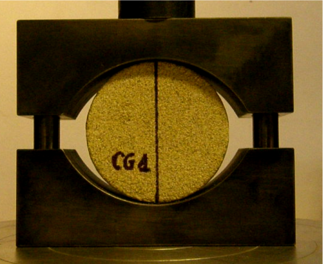
The Brazilian (splitting) indirect tensile strength test Simpson2014 has been performed on two rock types - Castlegate sandstone (CG) and Mons chalk (MC). Both rocks have a fairly homogeneous and isotropic (with no distinct layering) structure. The specimens were cored perpendicular to bedding and cut into the discs of approximately $22$ mm thickness and $52$ mm diameter. Each disc was wrapped around the circumference with a masking tape. This softened the contact between the rock and the steel curved jaws (Fig. 1) within which the disc is clamped during the test. This curved jaws is then placed in a loading frame. We then continuously increase the externally applied load, at a very slow but constant speed of crosshead, until the failure of the sample occurs. In our experiment the external force is applied with a MTS load frame at the rate $0.003$ mm/Sec., until the failure of the material. The reaction force given by the sample is recorded at every time. Fracture development, indicated by the sudden drop in loading, is captured using a digital camera.

3 Experimental Results

Figure 3: Fracture patterns after failure. Top one is for Castlegate sandstone (CG) and the lower one is for Mons chalk (MC) samples.

Table 1: Details about the samples that we examined. The thickness/diameter ratio is $0.42$ for both of the samples.

Sample name	Weight	Diameter	Thickness
Castlegate sandstone	91.61gm.	52.26mm.	21.78mm.
Mons chalk	71.73gm.	51.75mm.	21.73mm.

Figure 4: (a) Square lattice of size $L=3$. Each point on the lattice is an element, follows Hooke’s law before the breaking point. A force $F_{0}$ is applied at the middle column from the top of the lattice. (b) Illustrates the effect of the applied force. Here it is assumed that the effect decreases linearly from the point of loading. The cut off length $L_{c}$ and the $F_{0}$ determines the slope of the decreasing force profile, slope $m$=-$F_{0}/L_{c}$.

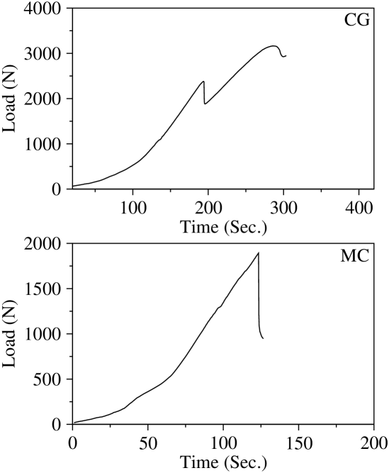
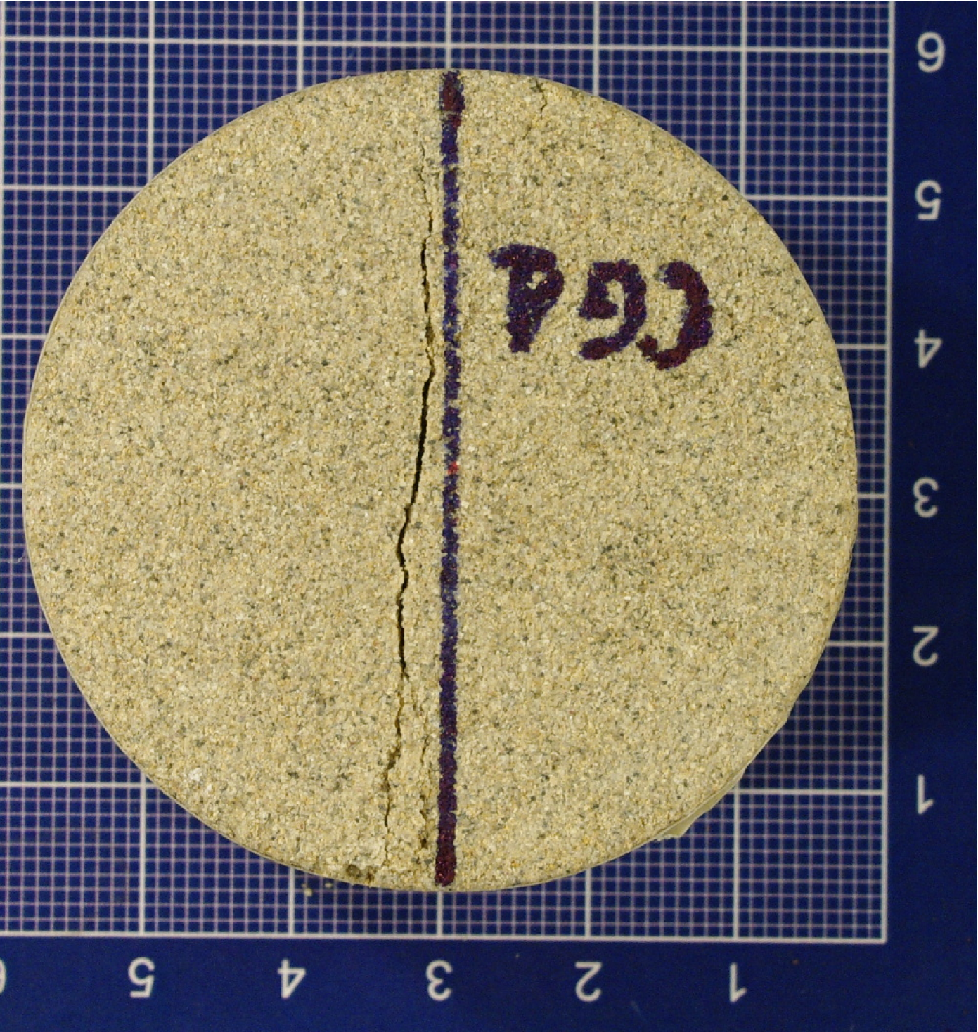
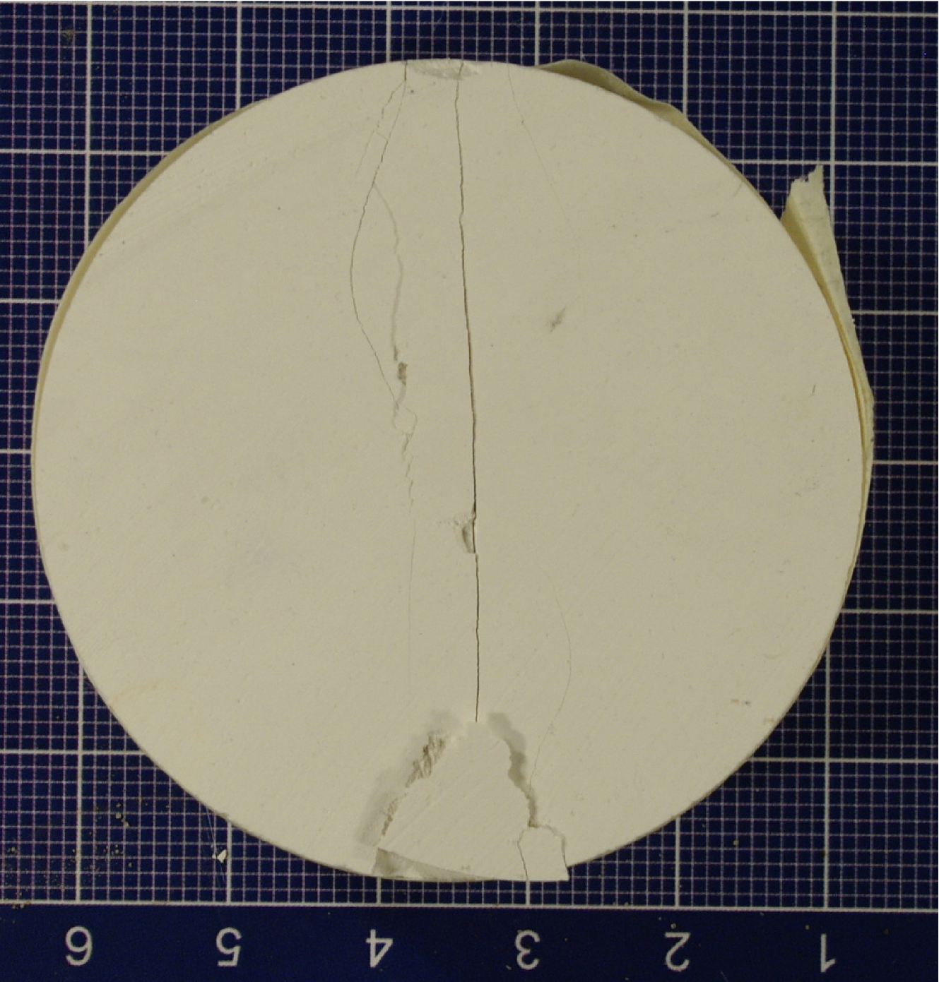
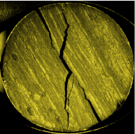
We experimentally examined the strength of two cylindrical samples CG and MC -masses and dimensions are given in the Table 1. In our experiment we increase the externally applied load on the material and measure the force with time. In Fig. 2 the load-time data has been plotted for both samples. The force/load values are measured in units of Newton (N). We define the tensile strength of material as the maximum load that a material can sustain without failure. For CG sample the first drop in the measured load at around 195 Sec., signifies the failure. When a fracture opens the near-by sand grains occupy the fractured region, also the contact area to the curved jaws broadens and thus the reaction force increases further. This is not observed in case of chalk sample due to the brittleness of the chalk. From the load-time plot it is obvious that the tensile strength of CG is greater than that of MC. In Fig. 3 the damage zone has been shown for both of the samples after the failure.

Figure 5: (a) For the uniformly distributed thresholds between $0.1$ to $1$ and $L_{c}=L/12$, the stress-strain behavior of a system with $L=64$ has been shown for three different values of strength decrement factor $\alpha=0.50$ (red), $\alpha=0.70$ (black) and $\alpha=0.90$ (blue). (b) The same data in (a) are plotted against the scaled variable $\varepsilon\alpha^{-0.92}$ and we obtain a reasonably good data collapse upto the failure point (the peak position).

4 Model

Figure 6: Crack profile for different values of the strength decrement factor, $\alpha$, right at the point where the stress-strain curve reached it’s maximum. The black color represents the intact elements and the white patches at the middle of it are the broken elements within the system of size $L=64$. Here the thresholds are distributed uniformly between $0.1$ to $1$ and in simulation we used $L_{c}=L/12$.

Our model consists of Hookean elements, placed on each lattice point of a regular square lattice, with their own breaking thresholds drawn randomly from a given probability distribution. Once the load on an element exceeds its breaking threshold, it breaks immediately and the load capacity of its neighboring intact elements are decreased indicating the weakening effect around the defected zone. One may think of the redistribution of load carried by the broken element among the intact elements as in the case of fiber bundle model Hansen2015 ; Pradhan2010 . In our model the load experienced by the intact elements are kept constant throughout the breaking process, elements break only due to the decrement of their breaking thresholds. To model the Brazilian test, the external load is applied at the middle point of the system and it is assumed that the effect of the applied force diminishes linearly as we move-on horizontally in either sides from the point of loading. From this model we numerically investigate the breaking properties of the system.

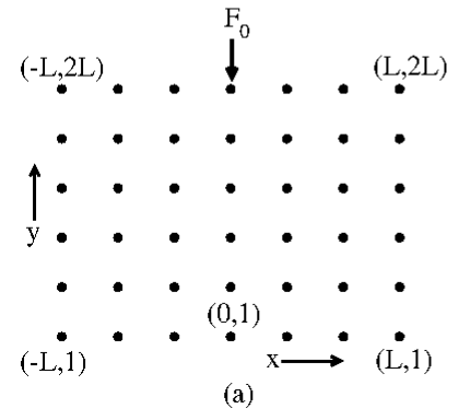
We consider a square lattice of size $L$ as shown in the Fig. 4(a). Each point on the lattice is an element. Each individual element positioned at $(x,y)$ has been assigned a breaking threshold $b_{(x,y)}$ i.e., it can sustain a maximum $b_{(x,y)}$ amount of load through it, beyond which it breaks irreversibly. Before breakdown each element follows Hooke’s law. For simplicity we assume the stiffness factor of all the elements to be unity. The breaking thresholds $\{b_{(x,y)}\}$ are drawn from a probability distribution $p(b)$, the cumulative distribution of which is given by $P(b)=\int_{0}^{b}p(y)dy$. The breaking threshold distribution is the only source of disorder present in this model.

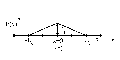
In our model we apply a force at the middle point of the lattice from the top of it, as shown in the Fig. 4(a). We assume that the effect of this applied force extends within a certain region from the point of application of the force. We consider the effect of this force decreases linearly and this force profile is symmetric about the point of loading. The force profile at the positive part of the lattice has the form:

$$F(x)=mx+F_{0}$$ (2)

and since it is symmetric about the point of loading so we have $F($-$x)=F(x)$. In Eqn. (2) $F_{0}$ is the amplitude of the applied force at the point $x=0$ and $m$ defines how far the effect of this applied force should extend. In our model we prefix a cut-off length $L_{c}$ beyond which the applied force has no effect i.e., $F(x)=0$ for $x>L_{c}$. This actually defines the value of $m($=-$F_{0}/L_{c})$. The whole schematic picture is depicted in the Fig. 4(b). We also assume that the load through all the elements of a particular column is same i.e., $F(x,y)=F(x)$.

An element breaks irreversibly and it’s neighborhood gets affected, when the force through the element exceeds it’s breaking threshold. When an element breaks, the breaking strength of it’s surviving nearest neighbors is decreased by a factor $\alpha(0\leq\alpha\leq 1)$, i.e., their new thresholds are assigned a value equal to $\alpha$ times of their own previous thresholds. This is actually the sense of weakening around the defected zone. The force profile remains unaltered in this model.

When a force is applied to the system, the breakdown of the elements occur from the middle part (close to the $x=0$) of the system since the force field is much stronger in this region. So, the local failures will grow from the middle zone of the system. This local failures decrease the strength of the elements around the defected zone. A local failure may occurs due to the weakness of the elements as well as due to the decrement of the strength of the elements after an failure event and due to this a spatial correlation develops in the failure events. Since the force field decreases linearly in the horizontal direction, it is more probable that failure will occur in the vertical direction. This makes cracks to propagate in the vertical up or vertical down direction rather than horizontal direction from the defected zone, which correlates with the experimental observations.

The width of disorder, the value of the cut-off length $L_{c}$ and the strength decrement factor $\alpha$ play a crucial role in the crack propagation. For a fixed window of disorder, smaller the value of $\alpha$ and $L_{c}$, lead successive failure to be more and more localized and directed in the vertical direction.

5 Numerical Results

We investigate the stress-strain behavior of the system which is the most crucial part of the Brazilian test. We observe the stress-strain behavior, the system size dependence of the maximum value of the stress and it’s fluctuation for both uniform and Weibull distribution of the breaking thresholds.

To obtain the stress-strain curve we increase the external load quasi-statically. Due to the loading all elements get stretched. At an elongation, $\varepsilon$ per intact element, the total force at a column is $\varepsilon$ times the total number of intact elements at the column. We define stress ($\sigma$) as-

$$\sigma=\frac{N_{in}\varepsilon}{2L}$$ (3)

where, $N_{in}$ is the number of intact elements at the central column.

Figure 7: (a) Plot of $\sigma_{c}(L)$ with $L$. The system size varies from $L=32$ to $L=1024$ with an increment of factor $2$. (b) Plot of $\sigma_{c}(L)$ with $L^{-0.4}$ is best fitted by a straight line, the extrapolation of which gives the value of $\sigma_{c}=0.14$.

Numerically, the stress-strain curve is obtained in the following way. Initially we start with a fully intact system and then we apply a load such that the weakest element in the system breaks. The weakest surviving element is determined by calculating the maximum of the ratio between force field to the breaking threshold i.e., $max\{F(x,y)/b_{(x,y)}\}$, which is equal to $max\{F(x)/b_{(x,y)}\}$. Once it is removed, the breaking strength of it’s nearest surviving neighbor is reduced by a factor $\alpha$. Due to this, it may so happen that the load through some of the elements exceed their breaking threshold and we break them simultaneously again reducing the strength of their neighboring elements, that may cause further breakdown and so on. This process stops when all the remaining intact elements have their breaking strength greater than their respective experienced stress values. We then increase the externally applied load in such a way that the weakest element among the remaining intact system reaches it’s breaking threshold and then the entire procedure is repeated. This procedure is continued until we are at a point well above the point where the maximum of the stress-strain curve takes place.

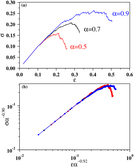
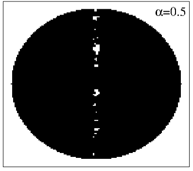
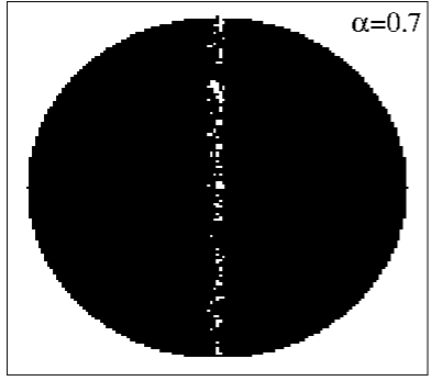
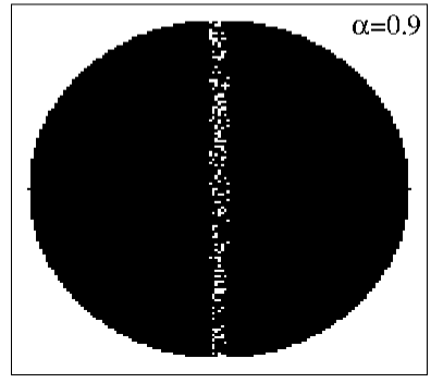
In Fig. 5(a) the stress-strain curve is shown for a particular configuration for different values of $\alpha$. In the next figure by suitably scale the abscissa and ordinate we could obtain a data collapse (Fig. 5(b)) upto the peak point. In experiments, after peak position, different rock samples behave differently -depending on their failure structure (clear fracture, complex fracture, crashed etc). Therefore, in our numerical study, we have tried the scaling up to the peak position. The defected zone right at the point where the stress-strain curve reaches it’s maximum has been shown by the white color in Fig. 6. Throughout the simulation we have used $L_{c}=L/12$.

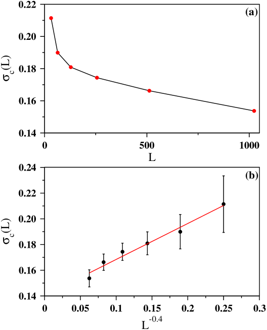
Once we generate the stress-strain curve, we then calculate the critical strength of the system. We define critical strength $\sigma_{c}^{s}(L)$ for a particular sample $s$ of size $L$ with a particular set of breaking thresholds $\{b_{(x,y)}\}$ as the maximum value of the stress in the stress-strain curve. For each sample $s$ we numerically calculate $\sigma_{c}^{s}(L)$ and when the whole procedure is repeated over a large number of uncorrelated samples, it eventually gives the average value of the critical strength $\sigma_{c}(L)=\langle\sigma_{c}^{s}(L)\rangle$ for the system of size $L$. We then repeat the entire set of calculation for different values of $L$ to know how $\sigma_{c}(L)$ approaches to it’s asymptotic value.

Figure 8: Log-log plot of $W(L)$ with $L$ for system size upto $L=512$. The fitted line has a slope $0.46$ and thus we conclude $W(L)\sim L^{-0.46}$.

Figure 9: (a) Plot of $\sigma_{c}(L)$ with $L^{-0.4}$. The best fitted straight line when extrapolated, it cuts the vertical axis at $0.24$ and thus the value of $\sigma_{c}=0.24$. Here the breaking threshold of the elements are drawn from the Weibull distribution of the form of Eqn. (6). (b) The fluctuation $W(L)$ varies with $L$ as- $W(L)\sim L^{-0.51}$.

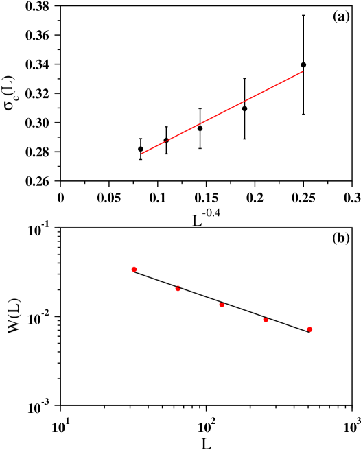
We assume that the average value $\sigma_{c}(L)$ for a system of size $L$ converges to it’s asymptotic value $\sigma_{c}=\sigma_{c}(\infty)$ as $L\rightarrow\infty$ according to the following form,

$$\sigma_{c}(L)=\sigma_{c}+AL^{-1/\nu}$$ (4)

For uniformly distributed breaking threshold of the elements in the range [$0.1$-$1.0$], the variation of $\sigma_{c}(L)$ against $L$ has been shown in Fig. 7(a). When the same $\sigma_{c}(L)$ values are plotted in Fig. 7(b) as a function of $L^{-1/\nu}$ with $1/\nu=0.40$, we observe that it can be fitted by a straight line. The least-squares fitted straight line cuts the vertical axis and has the form $\sigma_{c}(L)=0.14+0.28L^{-1/\nu}$. From here our conclusion is that $\sigma_{c}=0.14$ and $\nu=5/2$ for the uniformly distributed breaking thresholds.

We also measure the fluctuation of the critical strength, defined as-

$$W(L)=\sqrt{\langle\sigma_{c}(L)^{2}\rangle-\langle\sigma_{c}(L)\rangle^{2}}$$ (5)

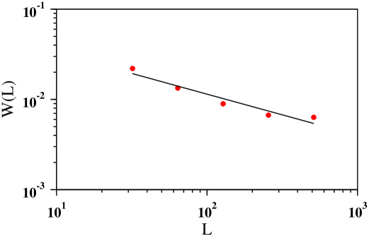
In Fig. 8 we plot $W(L)$ for different values of $L$ in log-log scale for the uniformly distributed breaking threshold and we observe that it decreases with increase in $L$. The best fitted line has a slope $0.46$.

We then repeat our entire set of studies for elements with Weibull breaking threshold distribution of the form:

$$P(b)=1-e^{-b^{2}}$$ (6)

We have estimated the values of $\sigma_{c}(L)$ numerically for six different system sizes from $32$ to $1024$ increased by a factor of $2$ at every step. Plotting them against $L^{-0.4}$ and extrapolating as $L\rightarrow\infty$ we have obtained $\sigma_{c}=0.24$. In Fig. 9(a) the plot of $\sigma_{c}(L)$ with $L^{-0.4}$ has been shown. Our conclusion is that for the Weibull distribution of breaking thresholds of the form of Eqn. (6), the value of $\sigma_{c}=0.24$ and $\nu=5/2$.

We also calculate $W(L)$ for different values of $L$ upto $L=512$. In Fig. 9(b) we plot the $W(L)$ as a function of $L$ and this is fitted with a straight line, resulting $W(L)\sim L^{-0.51}$.

6 Discussions and Conclusions

To model the Brazilian test we have introduced a statistical model and studied numerically the strength of the material. The stress-strain behavior of the system is found to have a maxima. We have investigated the critical strength of the system and also the system size dependence of the critical strength for both uniformly and Weibull distributed breaking threshold of the elements in the system. We observe that the damage profile right at the critical point (Fig. 6) resembles the nature of the damage profile observed in the Brazilian test experiment.

In our experiment, we have used the Brazilian test set up as indicated in Fig. 1. How the force field varies from the point of loading is entirely dependent on the shape and the material of the loading platen. For simplicity, we assume that the force decreases linearly from the tip point. It may also be possible to design loading plates where the gradient of the applied force follows power law or exponential. In our simulation we can easily include this type of force gradient along the loading plate. We believe that, it will have little effect on the nature of the final fracture pattern - because the main fracture initiates at and around the most stressed elements and after initial failure the newly created weak zones guide the fracture development. Therefore, as long as we have a force distribution on the system having a stress-tip and symmetrical gradient (decreasing) at both sides from the tip, we can expect similar fracture pattern.

For breaking thresholds distributed uniformly and with Weibull distribution, we observe that the critical strength $\sigma_{c}(L)$ of a system of size $L$ approaches the asymptotic values $0.14$ and $0.24$ respectively. For all the results obtained from our model, we have taken the strength decrement factor $\alpha=0.7$ and the cut-off length of the applied force $L_{c}=L/12$.

Figure 10: Snapshot of Brazilian test on an-isotropic shale sample at SINTEF lab Simpson2014

The stress-strain curve is very sensitive to the value of $\alpha$. In Fig. 5 the stress-strain behavior of a system with $L=64$ has been shown for three different values of $\alpha$. Lowering the value of $\alpha$ the more and more narrow, vertically directed and localized the damage zone become, shown in Fig. 6. As an effect the strength of the system will decrease. For $\alpha=1$ the behavior of this model is same as the mean field version of the Fiber Bundle model Hansen2015 ; Pradhan2010 ; Roy2013 , the elements break one by one with increasing sequence of their breaking thresholds.

Our statistical model is very simple in the sense -there are only two tuning parameters: the strength decrement factor $\alpha$ and the slope of the applied force/ load. According to the classical theory -stress fields are enhanced around the failure/ defect zones -which in turn weaken the elements in those areas. This fact has been captured in our model through the factor $\alpha$. The second parameter can be treated as an initial boundary condition which depends on the geometrical arrangements for the Brazilian test.

Recently Simpson et. al. has done a very interesting Brazilian test Simpson2014 on anisotropic rock sample (shale) and has monitored fracture development through high speed camera (See Fig. 10). Can we apply our model to simulate/explain such Brazilian test on highly anisotropic rocks Barla1973 ? The answer is yes. We can easily create weak bedding planes inside the model rock mass and we expect that in our model when the growing-fracture meets a weak plane - it must follow the direction of the weak plane unless it gets arrested by the presence of some strong elements. However we have to create the 3D version of our model first and then it needs a proper calibration against lab-experiments -which is our ongoing research activity.

The research work in this paper is a part of the scientific collaboration in the INDNOR project 217413/E20 funded by the Research Council of Norway. S. K. is thankful for financial support through the project grant to visit SINTEF Petroleum Research. We thank S. S. Manna for useful discussions. S.P. acknowledges partial support from SINTEF Petroleum Research through internal SIP project (7020606).

SK and SP implemented the model and performed the numerical analysis. AS set-up the experiment and performed the Brazilian test in presence of other two co-authors. All authors took part in developing the model, discussing the results and writing the paper.

References

- (1) D. Li and L. N. Y. Wong, Rock Mech. and Rock Eng. 46, 269 (2013).
- (2) M. Cai and P. K. Kaiser, Int. J. Rock Mech. and Min. Sci. 41, 478 (2004).
- (3) N. Erarslan and D. J. William, Int. J. Rock Mech. and Min. Sci. 49, 21 (2012).
- (4) M. K. Fahad, J. Mat. Sci. 31, 3723 (1996).
- (5) F. L. L. B. Carneiro, in Proceedings of the 5th meeting of the Brazilian Association for Technical Rules, 3d. section, (1943).
- (6) T. Akazawa, J. Japan Soc. Civil Eng. 29, 777 (1943).
- (7) ISRM, Suggested methods for determining tensile strength of rock materials, Int. J. Rock. Mech. and Min. Sci. and Geomech. Abstr. 15, 99 (1978) (DOI: 10.1016/0148-9062(78)90003-7).
- (8) N. D. J. Simpson, A. Stroisz, A. Bauer, A. Vervoort, and R. M. Holt, American Rock Mechanics Association 14, 7399 (2014).
- (9) M. Cai, Rock Mech. and Rock Eng. 46, 289 (2013).
- (10) D. F. Malan, J. A. L. Napier, and B. P. Watson, Int. J. Rock Mech. and Min. Sci. and Geomech. Abstr. 31, 581 (1994).
- (11) W. C. Zhu and C. A. Tang, Int. J. Rock Mech. and Min. Sci. 43(2), 236 (2006).
- (12) A. Hansen, P. C. Hemmer and S. Pradhan, in The Fiber Bundle Model: Modeling Failure in Materials, (Wiley-VCH, Berlin, 2015).
- (13) S. Pradhan, B. K. Chakrabarti and A. Hansen, Rev. Mod. Phys. 82, 499 (2010).
- (14) C. Roy, S. Kundu and S. S. Manna, Phys. Rev. E 87, 062137 (2013).
- (15) G. Barla and N. Innaurato, Rock Mech. and Rock Eng. 5, 215 (1973).