Error-Resilient Multicasting for Multi-View 3D Videos in Wireless Networks

Abstract

With the emergence of naked-eye 3D mobile devices, mobile 3D video services are becoming increasingly important for video service providers, such as Youtube and Netflix, while multi-view 3D videos have the potential to inspire a variety of innovative applications. However, enabling multi-view 3D video services may overwhelm WiFi networks when every view of a video are multicasted. In this paper, therefore, we propose to incorporate depth-image-based rendering (DIBR), which allows each mobile client to synthesize the desired view from nearby left and right views, in order to effectively reduce the bandwidth consumption. Moreover, when each client suffers from packet losses, retransmissions incur additional bandwidth consumption and excess delay, which in turn undermines the quality of experience in video applications. To address the above issue, we first discover the merit of view protection via DIBR for multi-view video multicast using a mathematical analysis and then design a new protocol, named Multi-View Group Management Protocol (MVGMP), to support the dynamic join and leave of users and the change of desired views. The simulation results demonstrate that our protocol effectively reduces bandwidth consumption and increases the probability for each client to successfully playback the desired views in a multi-view 3D video.

I Introduction

The IEEE 802.11 [1] WiFi standard has achieved massive market penetration due to its low cost, easy deployment and high bandwidth. Also, with the recent emergence of naked-eye 3D mobile devices, such as Amazon’s 3D Fire Phone, HTC’s EVO 3D, LG’s Optimus 3D, and Sharp’s Lynx, mobile 3D video services are expected to become increasingly important for video service providers such as Youtube and Netflix. In contrast to traditional stereo single-view 3D video formats, multi-view 3D videos provide users with a choice of viewing angles and thus are expected to stimulate the development of innovative applications in television, movies, education, and advertising [2]. Previous research on the deployment of 3D videos in wireless networks has mostly focused on improving 3D video quality for single-view 3D videos [3, 4], but multi-view 3D videos, which typically offer 5, 16 and 32 different viewing angels [5] have attracted much less attention.

Multi-View 3D videos are expected to significantly increase the network load when all views are transmitted. One promising way to remedy the bandwidth issue is to exploit depth-image-based rendering (DIBR) in mobile clients, in which the idea is to synthesize the desired view from one left view and one right view [2], because adjacent left and right views with a sufficiently small angle usually share many similar scenes and objects. Several schemes for bit allocation between the texture and depth map [6] and rate control with layered encoding for a multi-view 3D video [7] have been proposed to ensure that the quality of the synthesized view is very close to the original view (i.e., by minimizing total distortion or maximizing quality). Therefore, exploiting DIBR in clients eliminates the need to deliver every view of a video in a network. For practical situations, the computation overhead and extra energy consumption incurred by DIBR is small enough to be supported by current mobile devices [7, 8].For HTTP video streaming (ex., Youtube and MPEG-DASH) with TCP [9, 10], instead of UDP, DIBR can be performed when the views are waiting in the streaming buffer before playback.

Equipped with DIBR, only a subset of views are required to be multicasted in a network. However, multi-view 3D video multicast with DIBR brings new challenges in view selection for WiFi networks due to view synthesis and wireless erasure. Firstly, the number of skipped views between the left and right views in DIBR needs to be constrained to ensure the quality of the synthesized view [2]. In other words, since each transmitted view is multicasted to multiple clients, it is crucial to carefully select the transmitted views so that the desired view of each user can be synthesized with a left view and a right view close to each other. DIBR has a quality constraint [2], which specifies that the left and right views are allowed to be at most $R$ views away (i.e., $R-1$ views skipped between them) to ensure that every view between the left and right view can be successfully synthesized with good quality. Therefore, each new user cannot arbitrarily choose a left and a right view for synthesis with DIBR. The second challenge is that WiFi networks frequently suffer from wireless erasure, and different clients suffer from different loss probabilities due to varying channel conditions [11, 12, 13]. In 2D and single-view 3D videos, the view loss probability for each user can be easily derived according to the selected bit-rate, channel, and the setting of MIMO (e.g., antennas, spatial streams) in 802.11 networks. For multi-view 3D videos, however, when a video frame is lost for a user $i$ subscribing a view $k_{i}$, we observe that the left and right views multicasted in the network to other users can natively serve to protect view $k_{i}$, since the user $i$ can synthesize the desired view from the two views using DIBR. However, the view synthesis will fail if only one left view or one right view is received successfully by the client. Therefore, a new research problem is to derive the view failure probability, which is the probability that each user does not successfully receive and synthesize his/her desired view.

In this paper, we first analyze the view failure probability and compare it with the traditional view loss probability, which is the probability that a view fails to be sent to a user without DIBR. We then propose the Multi-View Group Management Protocol (MVGMP) for multi-view 3D multicast. When a user joins the video multicast group, it can exploit our analytical result to request the access point(AP) to transmit the most suitable right and left views, so that the view failure probability is guaranteed to stay below a threshold. On the other hand, when a user leaves the video multicast group, the proposed protocol carefully selects and withdraws a set of delivered views to reduce the network load, so that the video failure probability for other users will not exceed the threshold. Bandwidth consumption can be effectively reduced since it is not necessary to deliver all the views subscribed by the clients.

The rest of the paper is organized as follows. Section II describes the system model. Section III analyzes the view loss probability and view failure probability. Section IV presents the proposed protocol. Section V shows the simulation results, and Section VI concludes this paper.

II System Model

This paper considers single-cell video multicast in IEEE 802.11 networks, where the views transmitted by different bit-rates and on different channels are associated with different loss probabilities [11, 12, 13]. Currently, many video services, such as Youtube and Netflix, require reliable transmissions since Flash or MPEG DASH [9] are exploited for video streaming. Nevertheless, the current IEEE 802.2 LLC protocol for IEEE 802.11 networks does not support reliable multicast transmissions [14], and error recovery therefore needs to be handled by Layer-3 reliable multicast standards, such as PGM [15].

A multi-view 3D video can be encoded by various encoding schemes [16, 17]. Each view in a video consists of a texture image and a depth map of the corresponding viewing angle. The idea of DIBR is to synthesize a view according to its neighbor left view and neighbor right view. Since the angle between the neighbor left and right views is relatively small, it is expected that the video objects in the synthesized view can be warped (i.e., bent) from those in the two neighbor views. Effective techniques in computer vision and image processing have been proposed to ensure the video quality and limit the processing delay [18].

For example, suppose there are three multicast views, i.e., view 1, 3, and 4 subscribed by all clients. In the original WiFi multicast without DIBR, AP separately delivers each view in a multicast group to the corresponding clients, and three views are separately recovered or retransmitted during packet losses. In contrast, our approach enables a subscribed view to be synthesized by neighbor left and right views with DIBR, while the quality constraint in DIBR states that there are at most $R-1$ views between the neighbor left and right views, and $R$ can be set according to [2]. When $R=3$ in the above example, the lost of view 3 can be recovered by view 1 and 4, since view 3 can be synthesized by view 1 and 4 accordingly. In other words, a user can first try to synthesize the view according to the left view and right view when a subscribed view is lost, by joining the multicast groups corresponding to the left and right views.

The intuition behind our idea is traffic protection from neighbor views. A user can join more multicast groups to protect the desired view without extra bandwidth consumption in the network, because the nearby left view and right view may be originally multicasted to other users that subscribe the views. However, more unnecessary traffic will be received if the desired view is not lost, and the trade-off will be explored in the next section.

III Analytical Solution

In this section, we present the analytical results for multi-view 3D multicast in multi-rate multi-channel IEEE 802.11 networks with DIBR. We first study the scenario of single-view subscription for each user and then extend it to multi-view subscription. Table I summarizes the notations in the analysis. Based on the mathematical analysis, a new protocol is proposed in the next section to dynamically assign the proper views to each user.

III-A Single View Subscription

In single-view subscription, each user $i$ specifies only one desired view $k_{i}$. Each view can be sent once or multiple times if necessary. Let $p_{i,c,r}$ represent the view loss probability, which is the probability that user $i$ does not successfully receive a view under channel $c$ and bit-rate $r$. We define a new probability $P_{\varepsilon}^{(i)}$ for multi-view 3D videos, called view failure probability, which is the probability that user $i$ fails to receive and synthesize the desired view because the view and nearby left and right views for synthesis are all lost. In other words, the view loss probability considers only one view, while the view failure probability jointly examines the loss events of multiple views.

Theorem 1

In the theorem, we first explore the most generalized case studied in [19, 20, 21] with each multi-radio client able to operate on multiple channels simultaneously. For single-view subscription, the view failure probability for user $i$ is

$$P_{\varepsilon}^{(i)}=\prod_{c\in C_{i},r\in D_{i}}p_{i,c,r}^{n_{k_{i},c,r}}\times\Bigg{(}\mathbf{1}\{k_{i}=1\}+\mathbf{1}\{k_{i}=M\}\Bigg{)}$$

$$+\sum_{k=1}^{R-1}\Bigg{(}(1-\prod_{c^{\prime}\in C_{i},r^{\prime}\in D_{i}}p_{i,c^{\prime},r^{\prime}}^{n_{k_{i}-k,c^{\prime},r^{\prime}}})\prod_{l=1}^{\min(R-k,M-k_{i})}\prod_{\underset{c_{1},c_{2}\in C_{i}}{r_{1},r_{2}\in D_{i}}}$$

$$\prod_{q=0}^{k-1}p_{i,c_{1},r_{1}}^{n_{k_{i}-q,c_{1},r_{1}}}p_{i,c_{2},r_{2}}^{n_{k_{i}+l,c_{2},r_{2}}}\mathbf{1}\{M-1\geq k_{i}\geq k+1\}\Bigg{)}$$

$$+\prod_{q=0}^{\min(R-1,k_{i}-1)}\prod_{c_{3}\in C_{i},r_{3}\in D_{i}}p_{i,c_{3},r_{3}}^{n_{k_{i}-q,c_{3},r_{3}}}\mathbf{1}\{M-1\geq k_{i}\geq 2\}$$

where $\mathbf{1}\{\cdot\}$ denotes the indicator function.

Proof: The view failure event occurs when both of the following two conditions hold: 1) user $i$ does not successfully receive the desired view, and 2) user $i$ fails to receive any feasible set consisting of a left view and a right view with the view distance at most $R$ to synthesize the desired view. The probability of the first condition is $\prod_{c\in C_{i},r\in D_{i}}p_{i,c,r}^{n_{k_{i},c,r}}$ when the the desired view $k_{i}$ of user $i$ is transmitted by $n_{k_{i}}$ times. Note that if the desired view of user $i$ is view $1$ or view $M$, i.e., $k_{i}=1$ or $k_{i}=M$, user $i$ is not able to synthesize the desired view with DIBR, and thus the view failure probability can be directly specified by the first condition. For every other user $i$ with $M-1\geq k_{i}\geq 2$, we define a set of non-overlapping events $\{\mathcal{B}_{k}\}_{k=0}^{R-1}$, where $\mathcal{B}_{k}$ with $k>0$ is the event that the nearest left view received by user $i$ is $k_{i}-k$ , but user $i$ fails to receive a feasible right view to synthesize the desired view. On the other hand, $\mathcal{B}_{0}$ is the event that the user $i$ fails to receive any left view. Therefore, $\bigcup_{k=0}^{R-1}\mathcal{B}_{k}$ jointly describes all events for the second condition.

TABLE I: Notations in Analysis.

Description	Notation
$R$	Quality constraint of DIBR
$M$	Total number of views
$k_{i}$	The view desired by user $i$
$D_{i}$	A set of the available data rates for user $i$
$C_{i}$	A set of the available channels for user $i$
$n_{j,c,r}$	Number of multicast transmissions for view $j$
	transmitted by rate $r$ in the channel $c$
$p_{i,c,r}$	The view loss probability for user $i$ under
	channel $c$ and rate $r$
$P_{\varepsilon}^{(i)}$	The probability that user $i$ cannot obtain the
	desired view either by direct transmission or by
	DIBR
$p_{c,r}^{\text{AP}}(n)$	The probability that AP multicasts a view $n$ times
	under the channel $c$ and the rate $r$
$\alpha_{i}$	The percentage of the desired views that can be
	received or synthesized successfully by user $i$
$p_{\text{select}}$	The probability that a user selects each view

For each event $\mathcal{B}_{k}$ with $k>0$,

$$P(\mathcal{B}_{k})=(1-\prod_{c^{\prime}\in C_{i},r^{\prime}\in D_{i}}p_{i,c^{\prime},r^{\prime}}^{n_{k_{i}-k,c^{\prime},r^{\prime}}})\prod_{l=1}^{\min(R-k,M-k_{i})}$$

$$\prod_{\underset{c_{1},c_{2}\in C_{i}}{r_{1},r_{2}\in D_{i}}}\prod_{q=0}^{k-1}p_{i,c_{1},r_{1}}^{n_{k_{i}-q,c_{1},r_{1}}}p_{i,c_{2},r_{2}}^{n_{k_{i}+l,c_{2},r_{2}}}\mathbf{1}\{M-1\geq k_{i}\geq k+1\}$$

The first term $1-\prod_{c^{\prime}\in C_{i},r^{\prime}\in D_{i}}p_{i,c^{\prime},r^{\prime}}^{n_{k_{i}-k,c^{\prime},r^{\prime}}}$ indicates that user $i$ successfully receives view $k_{i}-k$, and the second term

$$\prod_{l=1}^{\min(R-k,M-k_{i})}\prod_{\underset{c_{1},c_{2}\in C_{i}}{r_{1},r_{2}\in D_{i}}}\prod_{q=0}^{k-1}p_{i,c_{1},r_{1}}^{n_{k_{i}-q,c_{1},r_{1}}}p_{i,c_{2},r_{2}}^{n_{k_{i}+l,c_{2},r_{2}}}$$

means that user $i$ does not successfully receive any left view between $k_{i}-k$ and $k$ and any right view from $k_{i}+1$ to $k_{i}+\min(R-k,M-k_{i})$. It is necessary to include an indicator function in the last term since $\mathcal{B}_{k}$ will be a null event if $k_{i}\leq k$, i.e., user $i$ successfully receives a view outside the view boundary. Finally, the event $\mathcal{B}_{0}$ occurs when no left view is successfully received by user $i$.

$$P(\mathcal{B}_{0})=$$

$$\prod_{q=0}^{\min(R-1,k_{i}-1)}\prod_{c_{3}\in C_{i},r_{3}\in D_{i}}p_{i,c_{3},r_{3}}^{n_{k_{i}-q,c_{3},r_{3}}}\mathbf{1}\{M-1\geq k_{i}\geq 2\}$$

The theorem follows after summarizing all events. $\blacksquare$

Remark: The advantage of a multi-view 3D multicast with DIBR can be clearly seen when comparing the view loss probability and view failure probability. The latter probability attaches a new term (i.e., the probability of $\bigcup_{k=0}^{R-1}\mathcal{B}_{k}$) to the view loss probability, where a larger $R$ reduces the probability of the second term. Equipped with DIBR, therefore, the view failure probability is much smaller than the view loss probability, see Section V.

For the case that each single-radio client can access only one channel and rate at any time, the theorem can be changed to the following one.

III-B Multiple View Subscription

In the following, we explore the case of a user desiring to subscribe to multiple views. We first study the following two scenarios: 1) every view is multicasted; 2) only one view is delivered for every $\widetilde{R}$ views, $\widetilde{R}$ $\leq R$, and thus it is necessary for a user to synthesize other views accordingly. We first define $\alpha_{i}$, which represents the percentage of desired views that can be successfully received or synthesized by user $i$.

$$\alpha_{i}=\frac{\sum_{k_{i}\in\mathcal{K}_{i}}\mathbf{1}\{\text{user }i\text{ can obtain view }k_{i}\}}{|\mathcal{K}_{i}|}$$

where $\mathcal{K}_{i}$ denotes the set of desired views for user $i$. By using Theorem 1, we can immediately arrive at the following corollary.

Corollary 1

$$\mathbb{E}[\alpha_{i}]=\frac{\sum_{k_{i}\in\mathcal{K}_{i}}(1-P_{\varepsilon}^{(i)}(k_{i}))}{|\mathcal{K}_{i}|}$$ (1)

where $P_{\varepsilon}^{(i)}(k_{i})$ is given in Theorem 1.

Proof:

$$\mathbb{E}[\alpha_{i}]= \frac{\sum_{k_{i}\in\mathcal{K}_{i}}\mathbb{E}\mathbf{1}\{\text{user }i\text{ can obtain view }k_{i}\}}{|\mathcal{K}_{i}|}$$

$$= \frac{\sum_{k_{i}\in\mathcal{K}_{i}}(1-P_{\varepsilon}^{(i)}(k_{i}))}{|\mathcal{K}_{i}|}$$

$\blacksquare$

Eq. (1) becomes more complicated as $|\mathcal{K}_{i}|$ increases. In the following, therefore, we investigate the asymptotic behavior of $\alpha_{i}$ for a large $|\mathcal{K}_{i}|$ and a large $M$ (i.e., $|\mathcal{K}_{i}|\leq M$). To find the closed-form solution, we first consider a uniform view subscription and assume that user $i$ subscribes to each view $j$ with probability $p_{\text{select}}=\frac{|\mathcal{K}_{i}|}{M}$ independently across all views so that the average number of selected views is $|\mathcal{K}_{i}|$. Assume the AP multicasts view $j$ in channel $c$ with rate $r$ by $n$ times with probability $p_{j,c,r}^{\text{AP}}(n)$ independently across all views, channels, and rates. In the following, we first perform the asymptotic analysis to derive the theoretical closed-form solution, and we then present the insights from the theorem by comparing the results of single-view subscription and multi-view subscription.

Theorem 2

In multi-view 3D multicast,

$$\alpha_{i}(\mathcal{K}_{i})\overset{a.s.}{\rightarrow} (1-p_{i})\Bigg{\{}\sum_{k=1}^{R}k(1-p_{i})p_{i}^{k-1}+p_{i}^{R}\Bigg{\}}$$ (2)

$$\mathbb{E}[\alpha_{i}(\mathcal{K}_{i})]\overset{a.s.}{\rightarrow} (1-p_{i})\Bigg{\{}\sum_{k=1}^{R}k(1-p_{i})p_{i}^{k-1}+p_{i}^{R}\Bigg{\}}$$ (3)

as $|\mathcal{K}_{i}|\rightarrow\infty$, where $p_{i}=\prod_{c\in C_{i},r\in D_{i}}\sum_{n}p_{c,r}^{\text{AP}}(n)p_{i,c,r}^{n}$

Proof: We first derive the view loss probability for user $i$. Suppose that the AP multicasts a view $n$ times via channel $c$ and rate $r$. The probability that user $i$ cannot successfully receive the view is $p_{i,c,r}^{n}$. Because the AP will multicast a view $n$ times via channel $c$ and rate $r$ with probability $p_{c,r}^{\text{AP}}(n)$, the probability that user $i$ cannot receive the view via channel $c$ and rate $r$ is $\sum_{n}p_{c,r}^{\text{AP}}(n)p_{i,c,r}^{n}$. Therefore, the view loss probability for user $i$ is the multiplication of the view loss probabilities in all channels and rates, i.e., $\prod_{c\in C_{i},r\in D_{i}}\sum_{n}p_{c,r}^{\text{AP}}(n)p_{i,c,r}^{n}$. For simplification, we denote $p_{i}$ as the view loss probability for user $i$ in the remainder of the proof.

Since the multicast order of views is not correlated to $\alpha_{i}$, we assume that the AP sequentially multicasts the views from view $1$ to view $M$. Now the scenario is similar to a tossing game, where we toss $M$ coins, and a face-up coin represents a view successfully received from the AP. Therefore, the face-up probability of at least one coin is $1-p_{i}^{M}$. Now we mark a coin with probability $p_{\text{select}}$ if it is face-up or if there is one former tossed face-up coin and one latter tossed face-up coin with the view distance at most $R$. Since the above analogy captures the mechanism of direct reception and DIBR of views, the marked coins then indicate that the views selected by user $i$ can be successfully acquired.

To derive the closed-form asymptotic result, we exploited the delayed renewal reward process, in which a cycle begins when a face-up coin appears, and the cycle ends when the next face-up coin occurs. The reward is defined as the total number of marked coins. Specifically, let $\{N(t):=\sup\{n:\sum_{i=0}^{n}X_{i}\leq t\},t\geq 0\}$ denote the delayed renewal reward process with inter-arrival time $X_{n}$, where $X_{n}$ with $n\geq 1$ is the time difference between two consecutive face-up coins, and $X_{0}$ is the time when the first face-up coin appears.

Let $R(M)$ and $R_{n}$ denote the total reward earned at the time $M$, which corresponds to the view numbers in a multi-view 3D video. At cycle $n$,

$$\frac{R(M)}{M}=\frac{\sum_{n=1}^{N(M)}R_{n}}{M}+o(1)~{}~{}~{}a.s.$$

where the $o(1)$ term comes from the fact that the difference between the total reward and $\sum_{n=1}^{N(M)}R_{n}$ will have a finite mean. Recall that the reward earned at each cycle is the number of marked coins,

$$\mathbb{E}[R_{n}|X_{n}]= p_{\textrm{select}}, X_{n}>R$$ for

$$\mathbb{E}[R_{n}|X_{n}]= X_{n}p_{\textrm{select}}, X_{n}\leq R$$ for (4)

since when $X_{n}\leq R$, $X_{n}$ coins can be marked (each with probability $p_{\text{select}}$) between two consecutive face-up coins, and thus the expected reward given $X_{n}$ is $X_{n}p_{\text{select}}$. By contrast, only one coin can be marked with probability $p_{\text{select}}$ when $X_{n}>R$, and the expectation of reward given $X_{n}$ is only $p_{\text{select}}$.

Since $X_{n}$ is a geometric random variable with parameter $1-p_{i}$, we have

$$\mathbb{E}[X_{n}]=1-p_{i}+2p_{i}(1-p_{i})+3p_{i}^{2}(1-p_{i})+\cdots=\frac{1}{1-p_{i}}$$

and

$$\mathbb{E}[R_{n}]= p_{\text{select}}(1-p_{i})+2p_{\text{select}}p_{i}(1-p_{i})+\cdots$$

$$+Rp_{\text{select}}p_{i}^{R-1}(1-p_{i})+p_{\text{select}}p_{i}^{R}$$ (5)

By theorem 3.6.1 of renewal process in [22],

$$\frac{\sum_{n=1}^{N(M)}R_{n}}{M} \overset{a.s.}{\rightarrow}\frac{\mathbb{E}R_{n}}{\mathbb{E}X_{n}}$$

$$=p_{\text{select}}(1-p_{i})\Bigg{\{}\sum_{k=1}^{R}k(1-p_{i})p_{i}^{k-1}+p_{i}^{R}\Bigg{\}}$$ (6)

Let $U_{M}$ denote the number of views selected by user $i$. Therefore,

$$\alpha_{i}=\frac{R(M)}{U_{M}}=\frac{R(M)}{M}\frac{M}{U_{M}}$$

For $\frac{U_{M}}{M}\overset{a.s.}{\rightarrow}p_{\text{select}}$, by the strong law of large numbers, after combining with Eq. (4), (5), (6),

$$\alpha_{i}\overset{a.s.}{\rightarrow}(1-p_{i})\Bigg{\{}\sum_{k=1}^{R}k(1-p_{i})p_{i}^{k-1}+p_{i}^{R}\Bigg{\}}$$

The proof for convergence in mean is similar. It is only necessary to replace the convergence in Eq. (6) by the convergence in mean, which can be proven by the same theorem. $\blacksquare$

Remark: Under the above uniform view subscription, it can be observed that $\alpha_{i}$ is irrelevant to $p_{\text{select}}$, implying that different users with different numbers of subscription will acquire the same percentage of views. Most importantly, $\alpha_{i}=1-p_{i}$ for multi-view 3D multicasts without DIBR. In contrast, multi-view 3D multicasting with DIBR effectively improves $\alpha_{i}$ by $\sum_{k=1}^{R}k(1-p_{i})p_{i}^{k-1}+p_{i}^{R}$. Since this term is strictly monotonically increasing with $R$, we have $\sum_{k=1}^{R}k(1-p_{i})p_{i}^{k-1}+p_{i}^{R}>\sum_{k=1}^{1}k(1-p_{i})p_{i}^{k-1}+p_{i}=1$, which implies that the percentage of obtained views is strictly larger in statistic term s by utilizing the DIBR technique.

In the following, we consider the second case with only one view delivered for every $\widetilde{R}$ view, where the bandwidth consumption can be effectively reduced. Note that the following corollary is equivalent to Theorem 2 when $\widetilde{R}=1$.

Corollary 2

If the AP only transmits one view with probability $p_{c,r}^{\text{AP}}(n)$ for every $\widetilde{R}$ views,

$$\alpha_{i}(\mathcal{K}_{i})\overset{a.s.}{\rightarrow} \frac{(1-p_{i})\Bigg{\{}\sum_{k=1}^{\lfloor\frac{R}{\widetilde{R}}\rfloor}\widetilde{R}k(1-p_{i})p_{i}^{k-1}+p_{i}^{\lfloor\frac{R}{\widetilde{R}}\rfloor}\Bigg{\}}}{\widetilde{R}}$$ (7)

$$\mathbb{E}[\alpha_{i}(\mathcal{K}_{i})]\rightarrow \frac{(1-p_{i})\Bigg{\{}\sum_{k=1}^{\lfloor\frac{R}{\widetilde{R}}\rfloor}\widetilde{R}k(1-p_{i})p_{i}^{k-1}+p_{i}^{\lfloor\frac{R}{\widetilde{R}}\rfloor}\Bigg{\}}}{\widetilde{R}}$$ (8)

as $|\mathcal{K}_{i}|\rightarrow\infty$, where $p_{i}=\prod_{c\in C_{i},r\in D_{i}}\sum_{n}p_{c,r}^{\text{AP}}(n)p_{i,c,r}^{n}$

IV Protocol Design

For a multi-view 3D multicast, each view sent in a channel with a rate is associated with a multicast group. Based on the analytical results in Section III, each client subscribes to a set of views by joining a set of multicast group, in order to satisfy the view failure probability. To support the dynamic join and leave of users and the change of the subscribed views, we present a new protocol, named Multi-View Group Management Protocol (MVGMP), which exploits the theoretical results in Section III. The MVGMP protocol extends the current IETF Internet standard for multicast group management, the IGMP [23], by adding the view selection feature to the protocol. The IGMP is a receiver-oriented protocol, where each user periodically and actively updates its joined multicasting groups to the designated router (i.e., the AP in this paper).

In MVGMP, the AP maintains a table, named ViewTable, for each video. The table specifies the current multicast views and the corresponding bit-rates and channels for each view, and each multicast view is associated with a multicast address and a set of users that choose to receive the view. ViewTable is periodically broadcasted to all users in the WiFi cell. The MVGMP includes two control messages. The first message is Join, which contains the address of a new user and the corresponding requested view(s), which can be the subscribed views, or the left and right views to synthesize the subscribed view. An existing user can also exploit this message to update its requested views. The second message is Leave, which includes the address of a leaving user and the views that no longer need to be received. An existing user can also exploit this message to stop receiving a view. Following the design rationale of the IGMP, the MVGMP is also a soft-state protocol, which implies that each user is required to periodically send the Join message to refresh its chosen views, so that unexpected connection drops will not create dangling states in ViewTable.

Join. When a new member decides to join a 3D video multicast transmission, it first acquires the current ViewTable from the AP. After this, the user identifies the views to receive according to Theorem 1. Specifically, the client first examines whether ViewTable has included the subscribed view. If ViewTable does not include the subscribed view, or if the view loss probability for the subscribed view in the corresponding channel and bit-rate exceeds the threshold, the user adds a left view and a right view that lead to the maximal decrement on the view failure probability. To properly select the views, The user can search the view combinations exhaustively with the theoretical results in Section III, because R is small and thus only a small number of views nearby to the desired view is necessary to be examined. However, a view cannot be added to a channel without sufficient bandwidth.

When a multi-view 3D video starts, usually the current multicast views in ViewTable are not sufficient for a new user. In other words, when the view failure probability still exceeds the threshold after the user selects all transmitted left and right views within the range $R$ in ViewTable, the user needs to add the subscribed view to ViewTable with the most suitable channel and bit-rate to reduce the view failure probability. Also, the left and right views are required to be chosen again according to the analytic results in Section III to avoid receiving too many views. After choosing the views to be received, a Join message is sent to the AP. The message contains the views that the user chooses to receive, and the AP adds the user to ViewTable accordingly. To avoid receiving too many views, note that a user can restrict the maximum number of left and right views that are allowed to be received and exploited for DIBR.

Leave and View Re-organization. On the other hand, when a user decides to stop subscribing to a multi-view 3D video, it multicasts a Leave message to the AP and to any other user that receives at least one identical view $k_{i}$. Different from the Join message, the Leave message is also delivered to other remaining users in order to minimize the bandwidth consumption, since each remaining user that receives $k_{i}$ will examine if there is a chance to switch $k_{i}$ to another view $\overline{k}_{i}$ that is still transmitted in the network. In this case, the remaining user also sends a Leave message that includes view $k_{i}$, together with a Join message that contains view $\overline{k}_{i}$. If a view is no longer required by any remaining users, the AP stops delivering the view. Therefore, the MVGMP can effectively reduce the number of multicast views.

Discussion. Note that the MVGMP can support the scenario of a user changing the desired view, by first sending a Leave message and then a Join message. Similarly, when a user moves, thus changing the channel condition, it will send a Join message to receive additional views if the channel condition deteriorates, or a Leave message to stop receiving some views if the channel condition improves. Moreover, when a user is handed over to a new WiFi cell, it first sends a Leave message to the original AP and then a Join message to the new AP. If the network connection to a user drops suddenly, the AP removes the information corresponding to the user in ViewTable when it does not receive the Join message (see soft-state update as explained earlier in this section) for a period of time. Therefore, the MVGMP also supports the silent leave of a user from a WiFi cell. Moreover, our protocol can be extended to the multi-view subscription for each client by replacing Theorem 1 with Theorem 2. The fundamental operations of Join/Leave/Reorganize remain the same since each view is maintained by a separate multicast group.

V Simulation Results

In the following, we first describe the simulation setting and then compare the MVGMP with the current multicast scheme.

V-A Simulation Setup

We evaluate the channel time of the MVGMP in a series of scenarios with NS3 802.11n package. The channel time of a multicast scheme is the average time consumption of a frame in WiFi networks. To the best knowledge of the authors, there has been no related work on channel time minimization for multi-view 3D video multicast in WiFi networks. For this reason, we compare the MVGMP with the original WiFi multicast scheme, in which all desired views are multicasted to the users.

We adopt the setting of a real multi-view 3D dataset Book Arrival [5] and the existing multi-view 3D videos [24] with 16 views, where the texture video quantization step is 6.5, and depth map quantization step is 13, and the PSNR of the synthesized views in DIBR is around 37dB [25]. The video rates for reference texture image and its associated depth map are assigned as $r_{t}=600$kbps and $r_{d}=200$kbps, respectively, and thus $r=800$ kbps. The DIBR quality constraint is 3, $R=3$. The threshold of each user is uniformly distributed in (0, 0.1]. Each user randomly chooses one preferred view from three preference distributions: Uniform, Zipf, and Normal distributions. There is no specifically hot view in the Uniform distribution. In contrast, the Zipf distribution, $f(k;s;N)=(\frac{1}{k^{s}})/\sum_{n=1}{N}(\frac{1}{n^{s}})$, differentiates the desired views, where $k$ is the preference rank of a view, $s$ is the the exponent characterizing the distribution, and $N$ is the number of views. The views with smaller ranks are major views and thus more inclined to be requested. We set $s=1$ and $N=|V|$ in this paper. In the Normal distribution, central views are accessed with higher probabilities. The mean is set as $|V|/2$, and the variance is set as 1 throughout this study.

We simulate a dynamic environment with $50$ client users located randomly in the range of an AP. After each frame, there is an arrival and departure of a user with probabilities $\lambda$ and $\mu$, respectively. In addition, a user changes the desired view with probability $\eta$. The default probabilities are $\lambda=0.2$, $\mu=0.3$, $\eta=0.4$. TABLE II summarizes the simulation setting consisting of an 802.11n WiFi network with a 20MHz channel bandwidth and 13 orthogonal channels. In the following, we first compare the performance of the MVGMP with the current WiFi multicast scheme in different scenarios and then compare the analytical and simulation results.

TABLE II: Simulation Settings.

Parameter	Value
Carrier Frequency	5.0 GHz
The unit of Channel Time	$1ms$
Channel Bandwidth	20MHz
AP Tx Power	20.0 dBm
OFDM Data Symbols	7
Subcarriers	52
Video bit-rate(per view)	800kbps
Number of Orthogonal Channels	13
Transmission Data Rates	{6.5, 13, 19.5, 26, 39, 52, 58.5, 65}
	Mbps defined in 802.11n spec. [1]

The relationship between the setting of $R$ and the video quality has been studied in [2, 18]. Therefore, due to the space constraint, we focus on the channel time and view failure probability with different $R$ here, and the corresponding video quality can be derived according to [2, 18].

V-B Scenario: Synthesized Range

Fig. 1 evaluates the MVGMP with different settings of $R$. Compared with the current WiFi multicast, the channel time is effectively reduced in the MVGMP as $R$ increases. Nevertheless, it is not necessary to set a large $R$ because the improvement becomes marginal as $R$ exceeds 3. Therefore, this finding indicates that a small $R$ (i.e., limited quality degradation) is sufficient to effectively reduce the channel time in WiFi.

V-C Scenario: Number of Views

Fig. 2 explores the impact of the numbers of views in a video. The channel time in both schemes increases when the video includes more views, because more views need to be transmitted. This result shows that MVGMP consistently outperforms the original WiFi multicast scheme with different numbers of views in a video.

V-D Scenario: Number of Users in Steady State

Fig. 3 evaluates the channel time with different numbers of users in the steady state. We set $\lambda=\mu=0.25$, so that the expected number of users in the network remains the same. The channel time was found to grow as the number of users increases. Nevertheless, the increment becomes marginal since most views will appear in ViewTable, and thus more users will subscribe to the same views in the video.

V-E Scenario: Utilization Factor

Fig. 4 explores the impact of the network load. Here, we change the loading ratio $\rho:=\frac{\lambda}{\mu}$, i.e., the ratio between the arrival probability $\lambda$ and departure probability $\mu$. Initially, new multicast users continuously join the 3D video stream until the network contains 50 users. The results indicate that the channel time increased for both multicast schemes. Nevertheless, the MVGMP effectively reduces at least $40\%$ of channel time for all three distributions.

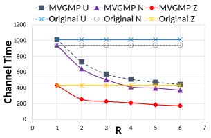
(a) Fig. 1: Synthesis Range

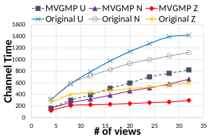
(b) Fig. 2: Number of Views in a Video

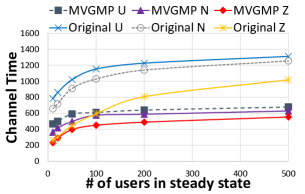
(c) Fig. 3: Number of Users

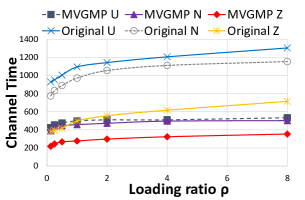
(d) Fig. 4: Network Load

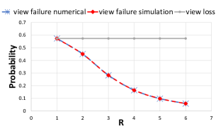
(e) Fig. 5: View Failure Probability

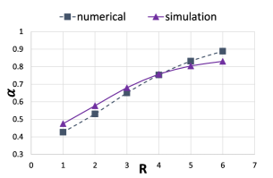
(f) Fig. 6: Ratio of Successfully Received Views

V-F Impact of User Preferences

From Fig. 1 to Fig. 4. the results clearly show that Uniform distribution requires the most channel time compared with Zipf and Normal distributions. This is because in Zipf and Normal distributions, users prefer a sequence of hot views, and those views thus have a greater chance to be synthesized by nearby views with DIBR.

V-G Analytical Result

Fig. 5 and Fig. 6 compare the simulation results from NS3 and the analytical results of Theorem 1 and Theorem 2 for the Uniform distribution, where each user subscribes to each view with a probability of 0.8. The results reveal that the discrepancy among the simulation and analysis is very small. Most importantly, $\alpha$ increases for a larger $R$ since each user can synthesize and acquire a desired view from more candidate right and left views when the desired view is lost during the transmissions.

VI Conclusion

With the emergence of naked-eye mobile devices, this paper proposes to incorporate DIBR for multi-view 3D video multicast in WiFi networks. We first investigated the merits of view protection via DIBR and showed that the view failure probability is much smaller than the view loss probability, while the multi-view subscription for each client was also studied. Thereafter, we proposed the Multi-View Group Management Protocol (MVGMP) to handle the dynamic joining and leaving for a 3D video stream and the change of the desired view for a client. The simulation results demonstrated that our protocol effectively reduces the bandwidth consumption and increases the probability for each client to successfully playback the desired view in a multi-view 3D video.

VII CoRR

To investigate the case where user subscribes a consecutive sequence of views, we adopt the following setting. User subscribes views according to a Zipf distribution, which means the $k$th view is subscribed with probability $\frac{c}{(k\textrm{ mod }m)^{s}}$ independently to other views. Figure$7$ depicts this scenario using $m=5$ as an example.

Following theorem serves as a counterpart of theorem $2$ in our main article.

Theorem 3

In the consecutive view subscription scenario as described above, the ratio $\widetilde{\alpha}$ of expected number of views that can be received or synthesized to the number of total subscribed views tends to

$$p\,\Bigg{\{}\sum_{j=1}^{m}\sum_{x=1}^{R}\Bigg{[}\Bigg{(}\sum_{l=1}^{m-j}\frac{c}{(j+l)^{s}}+\Bigg{(}\sum_{t=1}^{m}\frac{c}{t^{s}}\Bigg{)}\frac{x-(m-j)}{m}$$

$$+\sum_{l=1}^{[x-(m-j)]\textrm{mod }m}\frac{c}{l^{s}}\Bigg{)}p(1-p)^{x-1}\Bigg{]}\Bigg{\}}\Bigg{/}{\sum_{l=1}^{m}\frac{c}{l^{s}}}$$

as $|\mathcal{K}_{i}|\rightarrow\infty$, where $p=1-\prod_{c\in C_{i},r\in D_{i}}\sum_{n}p_{c,r}^{\text{AP}}(n)p_{i,c,r}^{n}$

Proof: We follow a similar arguments in our main article, which derives the theorem by reward theory. This time, however, we should use a generalized reward process, the Markov reward process. Let $T_{n}$ denote the index of the n-th successfully received view, and $G_{n}$ denote the state of the embedded Markov chain, which represents the ”position” of the n-th renewal cycle. An example of this definition is represented in figure. 7, in which the states of the first, second and the third cycles are $1,1,4$ respectively.

The transition probability of $G_{n}$ is

$$p_{ij} \frac{p(1-p)^{j-i-1}}{1-(1-p)^{m}}, 1\leq i<j\leq m$$

$$p_{ij} \frac{p(1-p)^{m-i+j-1}}{1-(1-p)^{m}}, 1\leq j\leq i\leq m$$ (9)

since, for example $1\leq i<j\leq m$, the position change from $i$ to $j$ occurs if and only if there are $j-i$ plus a multiple of $m$ views between the nearest two successfully received views, which means

$$p_{ij}=p(1-p)^{j-i-1}+p(1-p)^{j-i-1+m}+p(1-p)^{j-i-1+2m}+\cdots$$

The $\{(G_{n},T_{n}),n=1,2,3,\dots\}$ so defined is then a Markov renewal process.

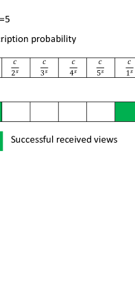
Figure 1: Fig. 7: Example of consecutive view subscription scenario

If we define the reward function of the process as $\rho(j,x)=$

$$\sum_{l=1}^{x}\mathbf{1(\textrm{view in the $l$ position has been subscribed})}, x\leq R$$

$$0, x>R$$

then

$$Z_{\rho}=\sum_{n:T_{n+1}<t}\rho(G_{n},T_{n+1}-T_{n})+\rho(G(t),X(t))$$ (10)

is a Markov reward process, where $X(t)$ is the age process and $G(t)$ be the semi-Markov process associated with our interested Markob renewal process $\{(G_{n},T_{n}),n=1,2,3,\dots\}$. The process so defined as the following desired property: The process just defined has a direct relation to our desired quantity $\widetilde{\alpha}$, which is

$$\widetilde{\alpha}=\frac{EZ_{\rho}}{S_{t}}$$

where $S_{t}$ is the number of views subscribed by the user. We now intend to apply the theorem 4.1 in [26] to the right hand side of the above equation. In the following, we will use the same notations as in the article just mentioned.

$$h(j) =\sum_{x=1}^{\infty}\rho(j,x)\sum_{j=1,2,\dots}P(G_{n+1}=j,T_{n+1}-T_{n}=x|G_{n}=i)$$

$$=\sum_{x=1}^{\infty}\rho(j,x)p(1-p)^{x-1}$$

$$=\sum_{x=1}^{R}\Bigg{[}\Bigg{(}\sum_{l=1}^{m-j}\frac{c}{(j+l)^{s}}+\Bigg{(}\sum_{t=1}^{m}\frac{c}{t^{s}}\Bigg{)}\,\frac{x-(m-j)}{m}\!$$

$$+\sum_{l=1}^{[x-(m-j)]\textrm{mod }m}\frac{c}{l^{s}}\Bigg{)}p(1-p)^{x-1}\Bigg{]}$$

Observe that the steady state of the chain $G_{n}$ is uniform distribution, which means

$$\pi_{i}=\frac{1}{m}$$ (12)

Now apply theorem 4.1 in [26], we have

$$\mathbb{E}Z_{\rho}(t)=pt\sum_{j=1,2,\dots}\pi_{j}h(j)+o(t)$$

Hence,

$$\frac{\mathbb{E}Z_{\rho}(t)}{S_{t}}\rightarrow mp\frac{\sum_{j=1,2,\dots}\pi_{j}h(j)}{\sum_{l=1}^{m}\frac{c}{l^{s}}}$$

$$=p\Bigg{\{}\sum_{j=1}^{m}\sum_{x=1}^{R}\Bigg{[}\Bigg{(}\sum_{l=1}^{m-j}\frac{c}{(j+l)^{s}}+\Bigg{(}\sum_{t=1}^{m}\frac{c}{t^{s}}\Bigg{)}\frac{x-(m-j)}{m}$$

$$+\sum_{l=1}^{[x-(m-j)]\textrm{mod }m}\frac{c}{l^{s}}\Bigg{)}p(1-p)^{x-1}\Bigg{]}\Bigg{\}}\Bigg{/}{\sum_{l=1}^{m}\frac{c}{l^{s}}}$$

References

- [1] IEEE, “Information Technology–Telecommunications and Information Exchange between Systems Local and Metropolitan Area Networks–Specific Requirements Part 11: Wireless LAN Medium Access Control (MAC) and Physical Layer (PHY) Specifications,” IEEE Standard, Mar. 2012.
- [2] Y. Mori, N. Fukushima, T. Yendo, T. Fujii, and M. Tanimoto, “View Generation with 3D Warping Using Depth Information for FTV,” Signal Processing: Image Communication, vol. 24, no. 1-2, pp. 65–72, Jan. 2009.
- [3] M. Nasralla, O. Ognenoski, and M. Martini, “Bandwidth Scalability and Efficient 2D and 3D Video Transmission over LTE Networks,” in IEEE International Conference on Communications, Jun. 2013, pp. 617–621.
- [4] B. Feitor, P. Assuncao, J. Soares, L. Cruz, and R. Marinheiro, “Objective Quality Prediction Model for Lost Frames in 3D Video over TS,” in IEEE International Conference on Communications, Jun. 2013, pp. 622–625.
- [5] I. Feldmann, M. Mueller, F. Zilly, R. Tanger, K. Mueller, A. Smolic, P. Kauff, and T. Wiegand, “HHI Test Material for 3-D Video,” Proc. 84th Meet. ISO/IEC JTC1/SC29/WG11, document M15413, Apr. 2008.
- [6] F. Shao, G. Jiang, M. Yu, K. Chen, and Y.-S. Ho, “Asymmetric Coding of Multi-View Video plus Depth based 3D Video for View Rendering,” IEEE Trans. on Multimedia, vol. 14, no. 1, pp. 157–167, Feb. 2012.
- [7] A. Hamza and M. Hefeeda, “Energy-Efficient Multicasting of Multiview 3D Videos to Mobile Devices,” ACM Trans. on Multimedia Computing, Communications, and Applications, vol. 8, no. 3s, pp. 45:1–45:25, Sep. 2012.
- [8] Y. Aksoy, O. Sener, A. Alatan, and K. Ugur, “Interactive 2D-3D Image Conversion for Mobile Devices,” in IEEE International Conference on Image Processing, Sep. 2012, pp. 2729–2732.
- [9] “Information Technology–Dynamic Adaptive Streaming over HTTP (DASH),” ISO/IEC 23009-1, Dec. 2014.
- [10] S. Alcock and R. Nelson, “Application Flow Control in YouTube Video Streams,” in SIGCOMM Computer Communication Review, Apr. 2011.
- [11] A. Sheth, S. Nedevschi, R. Patra, S. Surana, E. Brewer, and L. Subramanian, “Packet Loss Characterization in WiFi-Based Long Distance Networks,” in IEEE International Conference on Computer Communications, May 2007, pp. 312–320.
- [12] J. Feng, Z. Liu, and Y. Ji, “Wireless Channel Loss Analysis - a Case Study using WiFi-Direct,” in International Wireless Communications and Mobile Computing Conference, Aug. 2014, pp. 244–249.
- [13] A. Bose and H. F. Chuan, “A Practical Path Loss Model for Indoor WiFi Positioning Enhancement,” in International Conference on Information, Communications and Signal Processing, Dec. 2007, pp. 1–5.
- [14] IEEE, “Information Technology–Telecommunications and Information Exchange between Systems–Local and Metropolitan Area Networks–Specific Requirements–Part 2: Logical Link Control,” IEEE Standard, 1998.
- [15] T. Speakman et al., “PGM Reliable Transport Protocol Specification,” IETF RFC 3208, Dec. 2001.
- [16] H. Schwarz, D. Marpe, and T. Wiegand, “Overview of the Scalable Video Coding Extension of the H.264/AVC Standard,” IEEE Trans. on Circuits and Systems for Video Technology, vol. 17, no. 9, pp. 1103–1120, Sep. 2007.
- [17] A. Vetro, T. Wiegand, and G. Sullivan, “Overview of the Stereo and Multiview Video Coding Extensions of the H.264/MPEG-4 AVC Standard,” in Proceedings of the IEEE, vol. 99, no. 4, Apr. 2011, pp. 626–642.
- [18] G. Cheung, V. Velisavljevic, and A. Ortega, “On Dependent Bit Allocation for Multiview Image Coding with Depth-Image-Based Rendering,” IEEE Trans. on Image Processing, vol. 20, no. 11, pp. 3179–3194, Dec. 2011.
- [19] A. Raniwala and T. cker Chiueh, “Architecture and algorithms for an ieee 802.11-based multi-channel wireless mesh network,” in IEEE Computer and Communications Societies. (INFOCOM) Proceedings IEEE, vol. 3, March 2005, pp. 2223–2234 vol. 3.
- [20] M. Kodialam and T. Nandagopal, “Characterizing the capacity region in multi-radio multi-channel wireless mesh networks,” in Proceedings of the 11th Annual International Conference on Mobile Computing and Networking, ser. ACM MobiCom ’05, 2005, pp. 73–87.
- [21] T. Liu and W. Liao, “Interference-aware qos routing for multi-rate multi-radio multi-channel ieee 802.11 wireless mesh networks,” Wireless Communications, IEEE Transactions on, vol. 8, pp. 166–175, Jan 2009.
- [22] S. M. Ross, Stochastic Processes, 2nd ed. Wiley, 1983.
- [23] B. Cain et al., “Internet Group Management Protocol, ver. 3,” IETF RFC 3376, Oct. 2002.
- [24] K. M. P. Merkle, A. Smolic and T. Wiegand, “Multi-view video plus depth representation and coding,” in IEEE International Conference on Image Processing (IEEE ICIP), vol. 1, Sept 2007, pp. I – 201–I – 204.
- [25] Y. M. L. F. S. F. Z. Gaofeng, J. Gangyi and P. Zongju, “Joint video/depth bit allocation for 3d video coding based on distortion of synthesized view,” in IEEE International Symposium on Broadband Multimedia Systems and Broadcasting, Jun. 2012, p. 1–6.
- [26] A. R. Soltani and K. Khorshidian, “Reward processes for semi-markov processes: asymptotic behaviour,” Journal of Applied Probability, vol. 35, no. 4, pp. 833–842, 12 1998.